
Abstract
Organisms are often observed to acquire an excess of non-limiting resources, a process known as luxury consumption. Luxury consumption has been largely treated as a bet hedging strategy for temporal variation in resource supply, but may also function as a competitive strategy. We incorporate luxury resource consumption into a derivation of the classic resource ratio model for competition between terrestrial plant, and explore its consequences for population dynamics and competition. We show that luxury consumption reduces the potential for coexistence between two species competing for two resources. Furthermore, we demonstrate that luxury consumption can be selected for because of the competitive advantage that luxury consumers gain. Luxury consumption evolves when competition for resources is local rather than global, there is potential for coexistence between the two species and the competitive environment remains stable over a sufficient period of time to allow selection to act. The evolutionary outcome can be either extinction of one of the competing species or coexistence of the two species with maximum luxury consumption. The potential for selection to favor luxury consumption is well predicted by the competitive outcome between individuals of the two species with and without luxury consumption.
Introduction
Coexistence among species competing for limiting resources remains a central concern of community ecologists (e.g., Agrawal et al. 2007; Silvertown 2004). Resource ratio theory (Tilman 1982; Tilman 1988) is an important unifying body of theory with which to understand resource consumption and competition (Miller et al. 2005). An important simplifying attribute of the classic resource ratio model, however, is that resource uptake is limited to resources required for growth (Tilman 1982; Tilman 1988). The observation that organisms often acquire an excess of non-limiting resources, known as luxury consumption (Chapin et al. 1990), is at odds with this simplifying assumption. The focus of this paper is to relax this simplifying assumption, allowing luxury consumption of resources, in order to understand how this may affect predictions of stable coexistence under competition for limiting resources. We then proceed to explore the potential for luxury consumption to be selected for because of a competitive advantage it confers.
Empirical studies of luxury consumption argue that acquisition of excess nutrients is advantageous because these resources maybe stored for use when new inputs relieve constraints created by shortages of some other rate-limiting resource (Chapin et al. 1990). Luxury consumption, however, may also function as a competitive strategy. Preemptively sequestering resources may reduce the availability of a rate-limiting resource for competing species (van Wijk et al. 2003), a possibility that has not been assessed theoretically so far.
Luxury consumption is important to our understanding of coexistence under competition if it is a common attribute of species. Luxury consumption of non-rate-limiting resources was initially an empirical focus in plankton studies (Droop 1974; Droop 1983; Elrifi and Turpin 1985; Sterner and Schwalbach 2001; Stevenson and Stoermer 1982). In vascular plants, luxury consumption is most common in species growing from infertile habitats; they can show a high proportion of inorganic phosphorus and a low proportion of structurally bound P (Chapin 1980). Nitrogen and phosphorus are typically stored in vacuoles, as arginine and inorganic phosphate, respectively. The large vacuole storage reserves may represent 25–70% of total plant N and P (Chapin 1980). Lipson et al. (1996) document translocation from reserves accounting for 56% of the aboveground nitrogen requirement in a rhizomatous alpine herb. Recent work demonstrates that luxury consumption of resources occurs in many, but not all species, distributed across a wide array of vascular plant taxa, with typically species-specific responses (Boivin et al. 2004; Houle and Valery 2003; Lawrence 2001; Tripler et al. 2002). Furthermore, studies suggest that mycorrhizal association may play an important role in luxury consumption of resources (Koide 1991; Trent et al. 1993). Thus, empirical work suggests that luxury resource consumption is a common trait among terrestrial plant species, the group of taxa for which resource ratio models are most frequently applied.
With a single limiting nutrient, all models support the R* rule: the species that can decrease the limiting nutrient most wins competition (Grover 1997). There is support for the basic tenets of competitive exclusion and the resource ratio model in the phytoplankton literature: single limiting resources lead to extinction of one species; two species may coexist under particular nutrient supply rates when species are relatively more limited by different resources (Sommer 2002). Much of the phytoplankton literature has progressed to examine competition and evolutionary dynamics under variable environmental conditions (Ducobu et al. 1998; Grover 1991a; Grover 1991b; Grover 1997; Klausmeier et al. 2007; Sommer 2002), or stoichiometric constraints under different environmental conditions (Klausmeier et al. 2004a; Sterner and Elser 2002). There has been little work to examine the implications of luxury consumption on competition and coexistence in a stable environment; Tilman (1977) and Grover (1997) do, however, note that the predictions of the coexistence domain depend on the model. Revilla and Weissing (2008) show that a Droop model with nutrient storage show the same dynamics as models without storage, and Li and Smith (2007) show that these models result in the same competitive outcomes as a Lotka-Volterra competition model. Neither study explores the effect of storage on the coexistence domain. Thus, there has been little assessment of the effect of luxury consumption on competition, and no assessment of the potential for evolution of luxury consumption as a competitive strategy in a stable environment.
We chose to model luxury consumption using a simple two species, two resources framework that represents competition between terrestrial plants (Tilman 1982) in order to understand equilibrium dynamics and evolutionarily advantageous strategies with respect to luxury resource consumption. We assume that the two resources are two essential nutrients, such as nitrogen and phosphorus, that are limiting for growth. We relax the assumption that resource acquisition is limited by growth potential and allow luxury consumption as a constrained function of maximum nutrient uptake rate and biomass (Daufresne and Loreau 2001; DeAngelis 1992). We use our model to explore the effect of excess consumption on the predicted equilibrium outcome of competition. We next model the evolution of luxury consumption strategies in order to allow selection to act on strategies that maximize fitness. We assume that fitness is a function of biomass achieved through nutrient acquisition. We explore whether competition for limiting resources would select for luxury consumption of resources, or more appropriately preemptive resource consumption.
Model methods
General model
Consider a resource competition model for two species (A and B) competing for two limiting resources (R 1 and R 2) such as nitrogen and phosphorus. The following equations describe resource supply, uptake, and leaching (Daufresne and Loreau 2001; DeAngelis 1992; Tilman 1982) in a two-species competition model. The change in the amount of resource i, R i , where i is the resource index 1 or 2 is:
where S is the species index A or B, I i is input, l i is the leaching or loss rate, and g Si is the amount of nutrient i taken up by species S, a function of the useful biomass of species S, N S, and the availability of the two resources R 1 and R 2. All model variables and parameters are found in Table 1.
The change of resource i in biomass of species S, S i , is:
where m S is the tissue mortality rate. N S, is the amount of nutrient 1 incorporated into live biomass rather than storage; it thus measures the “useful” biomass of species S, that an individual can use for resource foraging:
where α S is the ratio requirement of the two nutrients for each species, so that under co-limitation of the two resources, or without luxury consumption, \( {\alpha_S} = \frac{{{R_2}{\text{ in biomass}}}}{{{R_1}{\hbox{ in biomass}}}} \).
Competition without luxury consumption
In the absence of luxury consumption, the two resources are taken up in proportion to the species’ ratio requirement α S:
Resource uptake is dependent upon biomass (N S ) and resource availability (R i ). In the absence of luxury consumption, the resource taken up is directly incorporated into biomass, and resource uptake follows a minimum function according to Liebig’s law of the minimum for two non-substitutable resources:
where f Si is the resource i uptake rate function for species S. Here we will consider specifically linear (f Si (R i ) = u Si R i ) and Monod type \( \left( {{f_{Si}}\left( {{R_i}} \right) = \frac{{u_{Si}^{\max }\,{R_i}}}{{{K_{Si}} + {R_i}}}} \right) \) uptake functions (Tables 1 and 2), as well as a generic function f Si that can be any monotonically increasing function. Note that the uptake kinetics for a nutrient is more efficient when it is limiting (uptake is then at the maximum value) than when it is non-limiting (where uptake is limited by the other, limiting nutrient), consistent with empirical observations (Turpin 1988a, b).
Planktonic systems are often modeled using Monod equations (Monod 1950), which set reproductive rates as a function of the availability of the more limiting nutrient, and nutrient uptake as a function of stoichiometric values, i.e., resource ratio requirement (Sterner and Elser 2002). In contrast, Droop (1973) proposed a variable internal stores model (Grover 1991b; Klausmeier et al. 2004a; Sommer 1991). Allowing internal storage of resources decouples species growth rates from nutrient concentration, and reproduction becomes dependent upon a cell quota of the more limiting resource (Smith and Waltman 1994). Empirical studies of resource competition can fit either the Monod or Droop models (Sommer 2002; Tilman 1977). Applied to several nutrients, the Droop model allows luxury consumption of the non-limiting nutrient. When applied to non-limiting nutrients, Klausmeier et al. (2004b) found a generally good fit of the Droop model, although Turpin (1988a, b) found it performed rather poorly. However, the applicability of Droop models to terrestrial plants is unclear. At equilibrium, a Droop model is equivalent to a Monod uptake function (Turpin 1988a, b), we therefore chose to proceed with our simpler, general uptake function.
Detailed analysis of this two species, two resource model can be found in Electronic supplementary material, section A. Species competitive ability for a limiting resource is defined by its ability to deplete a resource when limiting (\( R_{Si}^* \) for species S, resource i). Limiting resource depletion (\( R_{Si}^* \)) is the minimum level of the resource pool that allows the plant to maintain a positive growth rate and defines a zero net growth isocline (ZNGI, Fig. 1a). Its value depends on the species uptake and mortality parameters as shown in Table 2. From this basic modeling structure, Tilman (1982) demonstrated how various patterns in \( R_{Si}^* \) and resource requirements affect competitive outcomes and species coexistence (Fig. 1a, c, e). Two-species coexistence is predicted when each species requires more of the resource that is most limiting to that species (Fig. 1c, e; Tilman 1982), when resource supply is intermediate between the two resource consumption vectors (Fig. 1c). Extreme resource supply regions, of either resource, always result in competitive exclusion by one species or the other (Fig. 1c).

Competition for two resources as viewed by Tilman’s resource competition model (a, c, e), and adding maximum luxury consumption of resources (b, d, f). The x-axis represents the availability of resource 1, the y-axis represents the availability of resource 2. Both axes are scaled with loss rates (dilution rates in the case of a chemostat), so they are in units of resource per time unit (e.g., kg N ha−1 year−1). a A species is characterized by (1) its zero net growth isocline ZNGI that delimitates the regions of resource availability that lead to positive population growth (shaded areas) and (2) its resource ratio vector with slope α S, defining resource ratio requirement for population growth. For a given supply point (black dot), the species consumes the resource according to its resource requirement ratio, thus depleting the availability of the two resources until it reaches the ZNGI (equilibrium point *). Resource supply space which can be partitioned into two areas where each resource becomes the limiting factor, as indicated by shading. b Adding luxury consumption. At the interface between the two areas where each resource becomes limiting, the two resources are co-limiting, and a supply point on this interface (as I colim) results in the co-limitation equilibrium E colim. The slope from I colim to E colim is α S. For a linear uptake function, the intersections X 1 and X 2 between each axis and the resource acquisition vector that goes through the co-limitation equilibrium enable us to identify the equilibria with maximum luxury consumption. When resource 1 is limiting, the equilibrium reached with maximum luxury consumption is at the intersection between the ZNGI and the supply point −X 1 line. When resource 2 is limiting, the equilibrium reached with maximum luxury consumption is at the intersection between the ZNGI and the supply point—X 2 line. As in the classic resource competition model, we assume independence of resources with no positive or negative correlated consequences associated with resource acquisition. c–f Two-species competition. Species A is characterized by its ZNGI and resource acquisition vector (solid lines), and species B with dashed lines. The shading regions correspond to region of resource supply that lead to one of four possible competitive outcomes. When it exists, the two-species coexistence equilibrium point is at the intersection between the two-species ZNGIs. c and e Without luxury consumption; d and f With luxury consumption, corresponding scenarios to cases (c) and (e), respectively. The wide area of coexistence without luxury consumption are much reduced (compare c and d) or disappear (e and f) in the presence of luxury consumption. Note that other configurations could lead to a region of multiple stable states (MSS) without luxury consumption; this area would be widened by luxury consumption. Formulae for the ZNGIs and slopes of lines separating the different regions of the plot are in Table 2
Maximum luxury resource consumption
We allow species to engage in excess, or luxury, consumption of their less limiting resource in model (1–3). Our hypothesis is that when species engage in luxury consumption, they can pre-empt limiting resources from potential competitors and thereby reduce the conditions under which coexistence is predicted. This assessment is fundamentally distinct from the main focus of previous modeling efforts of luxury consumption in that most models have focused on excess nutrient uptake as a bet hedging strategy in a variable environment (Ducobu et al. 1998; Grover 1991a; Grover 1991b; Klausmeier et al. 2007), or the effect of luxury consumption on endogenous population fluctuations (Revilla and Weissing 2008). In contrast, we explore the evolution of luxury consumption as a competitive strategy.
We assume that a species can potentially acquire resources up to the maximum uptake rate displayed when the resource is limiting. Therefore, we constrain luxury resource acquisition as a function of maximum uptake functions. Under maximum luxury consumption, uptake of resource i by species S is thus:
which was incorporated in model (1–3). Note that under maximum luxury consumption, Eq. (5) does not apply, but Liebig’s law is still at work through the notion of “useful” biomass (Eq. 3).
Firstly, we analyzed the model with a single species, under maximum luxury consumption. Secondly, we analyzed the two-species competition model with maximum luxury consumption. Finally, we performed resource competition simulations between the two species. These simulations were repeated with maximum luxury consumption and without luxury consumption.
Intermediate levels of luxury consumption
Luxury consumption can be a continuous trait in-between the maximum or non-existent states modeled thus far. In order to understand whether selection would favor luxury consumption in an evolutionary model and how much luxury consumption would be selected for, we modeled intermediate amounts of luxury consumption along a continuum from zero to our modeled maximum (Table 1, Eq. 6). Uptake of resource 1 by an individual of species S with luxury consumption strategy lux is thus:
And uptake of resource 2 is:
Evolutionary dynamics of luxury consumption
In order to assess whether selection favors luxury consumption in an evolutionary model, we chose to model individuals interacting with other individuals in a pairwise simulation model. This model is in contrast to models where resources are pooled among all individuals, as if they were in a well-mixed homogeneous environment. From a resource modeling standpoint, in a well-mixed homogeneous environment where all individuals experience the same resource levels, luxury consumption has no effect on the fitness of its carrier: its useful growth is its maximum uptake of the limiting nutrient, \( \min \left( {{f_{S1}}\left( {{R_1}} \right),\frac{{{f_{S2}}\left( {{R_2}} \right)}}{{{\alpha_S}}}} \right) \). As a consequence the effect of luxury consumption becomes evolutionary neutral. Species-wide pooling of resources cannot select for luxury consumption for a competitive advantage because all individuals would share the benefit of the luxury consumption by any single individual. Terrestrial plants do not, however, interact globally with all others in their habitats. Taking into account a spatial context is necessary for the evolution of luxury consumption, but it potentially introduces new dimensions that strongly affect species coexistence and competitive exclusion: mortality and colonization dynamics (Tilman 1994), spatial scales of dispersal (Neuhauser and Pacala 1999; Pacala 1997) as well as spatial scales of competitive interactions (Murrell and Law 2003). To minimize these complications, we chose to investigate the evolution of luxury consumption in a dual lattice setting as used for the evolution of mutualism (Doebeli and Knowlton 1998; Travis et al. 2006; Yamamura et al. 2004). Each species population dynamics takes place on its own lattice, so the two species do not directly compete for space, but individuals compete for nutrients with their conspecific neighbors and their interspecific counterpart on the other lattice. The simulations we present here are even simpler: we assume that all lattice cells are occupied, that dispersal is global, and competition for nutrients just occur with the counterpart on the other lattice. We did preliminary investigations, not reported here, to investigate the effect of colonization and mortality (allowing sites to be empty), local dispersal, and competition for nutrients in a larger neighborhood and found the results to be generally consistent with those presented here.
In our model, pairs of competitors, one of each species, compete locally for nutrients. We define a number (Ls) of local sites in which two individuals, one of each species compete during the growth season. For each generation, each site is filled with one individual of each species drawn at random from a pool of propagules as in a lottery. Individuals are characterized by the amount of luxury consumption they conduct. Individuals of the two species grow together in each local site according to the dynamics of Eqs. (1–3 and 7–8). As a consequence, a single species, with some luxury consumption traits, will either win, lose, or coexist with the other species within that cell. Individuals with biomass above their reproductive threshold at the end of the growing season reproduce, so that the biomass above a given reproductive size is used to produce propagules. Offspring inherit their parent’s trait for luxury consumption, with a small probability of mutation, and they compete with other propagules of the same species to establish in a new cell at the next generation. Luxury consumption is a continuous trait between 0 (no luxury consumption) and 1 (maximum luxury consumption as defined above).
We allow luxury consumption attributes to change between each generation through mutation of the luxury consumption trait at reproduction. The rate at which the trait may mutate does not usually affect the outcome, but alters the rate at which the outcome is reached. We chose a 20% chance of carrying a mutation per propagule; the mutated luxury consumption trait is then drawn from a Gaussian distribution with mean trait value of the parent, and SD of 0.02. The distribution is truncated so that only values between 0 and 1 are allowed. At the end of each growing season, mean luxury consumption trait value and individual biomass are recorded for each species. Our evolutionary simulations stop when one of three outcomes occurs: (1) one of the two species goes extinct; (2) both species reach maximum luxury consumption: the median of luxury consumption is higher than 0.97; or (3) the simulation is timed out by running for 10,000 generations without extinction or reaching maximum luxury consumption.
For each simulation we drew each of our ten parameters that define ecological dynamics randomly from wide-ranging uniform distributions (see Table 1 for ranges). We selected those parameter sets where both species were able to survive on their own, and the ZNGIs of the species crossed (i.e., there is a trade-off between the ability of the two species to deplete the two resources). We selected these parameter conditions because fundamentally, we wanted to examine conditions under which luxury consumption would alter competitive outcomes.
We defined species A as best at depleting resource 1 and species B was best at depleting resource 2. We first used parameter sets as they were generated, but in order to have a fair representation of all different possible cases (Table 3), parameter sets were subsequently classified as a function of the expected equilibrium competitive outcome with and without luxury consumption and we ran more of the rarer cases. We ran simulation models of competitive dynamics starting with one propagule of each species both without luxury consumption and with maximum luxury consumption. Time to equilibrium was determined as the length of time (in ten time steps increments) after which running the model for an additional ten time steps would not lead to a change in any compartment larger than a small arbitrary number (10−2). When this criterion was met, the dynamics appeared to stabilize long before our determined time to equilibrium. We selected the 593 parameter sets, without and with luxury consumption, for which we could obtain equilibrium within 1,000 time units.
For each set of the selected parameters, we then modeled the evolutionary dynamics using one of two starting conditions. Firstly, we initiated simulations with propagules having no luxury consumption other than the probability of an initial mutation toward luxury consumption. In this case, we modeled competition in Ls = 200 local sites. Secondly, we initiated simulations with a set of 11 luxury consumption strategies uniformly distributed between 0 and 1 (0, 0.1, 0.2,..., 1) for each species, and paired between species with all possible combinations, yielding 121 pairs of strategies. In this case, we modeled competition in Ls = 121 local sites.
We ran the evolutionary model for two lengths of growing season: (1) a long growing season that allows the equilibrium to be reached; the determined time to equilibrium was used as length of the long growing season (see above) and (2) a shorter growing season at the end of which the dynamics often remains transient. As the equilibrium results are representative of our main conclusions, we only present those in the main manuscript (more details can be found in Electronic supplementary material, section B). Results of runs for the shorter growing season are shown in Electronic supplementary material, section C.
Results
-
1.
One-species equilibrium with maximum luxury consumption.
Maximum luxury consumption of resources can be depicted graphically (Fig. 1b). A single species has resource limitations that define its ZNGI, and a stoichiometric optimum uptake ratio (α S ). We then define an ideal resource supply line (Fig. 1b, semi-line from E colim towards I colim) such that resource uptake draws resources down to a joint minimum level of resources based on joint resource limitation: R S1 *,R S2 * (Fig. 1b, E colim). When resources fall on one side of this ideal resource supply line, or the other, one resource is more limiting than the other and some amount of luxury resource consumption is possible.
When there is limitation by resource 1, the equilibrium is (Table 2):
$$ {R_1}^* = {R_{A1}}^* = f_{A1}^{ - 1}\left( {{m_A}} \right) $$(9)$$ {R_2}^* = h_{A2}^{ - 1}\left( {{I_2}} \right) $$(10)where \( h_{A2}^{ - {1}} \) is the inverse of the function defined as: \( {h_A}_2\left( {{R_2}} \right) = {l_2}{R_2} + N_A^*{f_A}_2\left( {R{2}} \right) \). For a linear uptake function, we get \( {R_2}^* = \frac{{{I_2}}}{{\left( {{l_2} + {u_{A2}}{N_A}^*} \right)}} \); for a Monod uptake function, \( R_2^* \) is the positive solution of a second-degree equation: \( {R_2}^* = \frac{{\left( {{I_2} - {l_2}{K_{A2}} - u_{A2}^{\max }{N_A}^* + \sqrt {{4{I_2}{l_2}{K_{A2}} + {{\left( {{I_2} - {l_2}{K_{A2}} - u_{A2}^{\max }{N_A}^*} \right)}^2}}} } \right)}}{{2{l_2}}} \).
$$ {A_1}^* = {N_A}^* = \frac{{{I_1} - {l_1}{R_1}^*}}{{{m_A}}} $$(11)$$ {A_2}^* = \frac{{{f_{A2}}\left( {{R_2}^*} \right){N_A}^*}}{{{m_A}}} $$(12)The ratio of the two resources in biomass is then:
$$ \alpha_{A2}^{\rm{lux}} = \frac{{{A_2}^*}}{{{A_1}^*}} = \frac{{{f_{A2}}\left( {{R_2}^*} \right)}}{{{m_A}}} $$(13)In the case of a linear uptake function, the line between the resource supply (Fig. 1b, point I 1lim) and the equilibrium resource depletion point with luxury consumption (E 1lim lux) intersect with the ideal resource supply line (I colim − E colim) on the x-axis (intersection point X 1 in Fig. 1b; Electronic supplementary material, section A). This provides a simple geometric means to finding the equilibrium resource pools at equilibrium (Fig. 1b, E 1lim lux). Similar results are found when the species is limited by the other resource (Table 2).
Lacking luxury consumption, a species will consume resources in proportion to growth needs and deplete resources to its most limiting resource (Fig. 1b, from resource supply point I 1lim to equilibrium point E 1lim, from I colim to E colim, from I 2lim to E 2lim). Luxury consumption will result in depleting more of the non-limiting resource, sliding along the ZNGI. The difference between points E 2lim and E 2lim lux represents potential luxury consumption of resource 1 when resource 2 is limiting. Similarly, the difference between points E 1lim and E 1lim lux (Fig. 1b) represent potential luxury consumption of resource 2 under conditions when resource 1 is limiting.
-
2.
Equilibrium outcome of competition with maximum luxury consumption.
As without luxury consumption, competition can be understood by conditions under which other species may invade and persist. For a given resource supply, we allow species A to deplete the resources to its equilibrium point. Species B can invade if the resulting equilibrium lies in its region of positive growth. Repeating this exercise for the other species, we can partition the resource supply plane into regions in which one of the four following outcomes occur:
-
Species A outcompetes species B
-
Species B outcompetes species A
-
Coexistence (both can invade the other’s equilibrium), Fig. 1d.
-
Multiple Stable States, or founder effect: neither can invade the other at equilibrium so that the first one to settle outcompetes the other, Fig. 1f.
Space partitioning is explained in Electronic supplementary material, section B, and the slopes of the lines that make the partition are given in Table 2. For a linear uptake functional response, there is a simple geometrical construction of this partition (Fig. 1b; Electronic supplementary material, section B). Luxury consumption may thwart the existence of a potential competitor by drawing limiting resources below that which allows a stable two-species equilibrium. Thus, the conditions for coexistence without luxury consumption become much reduced with luxury consumption. This is illustrated in Fig. 1 by comparing the equivalent situations without (Fig. 1c, e) and with (Fig. 1d and f) maximum luxury consumption. In the first case, luxury consumption reduces the conditions for coexistence (Fig. 1c, d). In the second case, luxury consumption prevents coexistence that was possible in the absence of luxury consumption (Fig. 1e, f). Conditions that led to coexistence now lead to competitive exclusion, either deterministically or through a founder effect with multiple stable states (Fig. 2). Which species is excluded depends on their initial abundances (propagule size). In Fig. 2, species A has a small propagule size and loses in the alternative stable states configuration with maximum luxury consumption (Fig. 2d); an increased propagule size would enable this species to exclude species B, as illustrated in Fig. B2 in Electronic supplementary material. There are six possible configurations of parameter space partitioning, where each portion of space is one of nine possible combinations of competitive outcomes for the two species without and with luxury consumption (Electronic supplementary material, section B).
Fig. 2 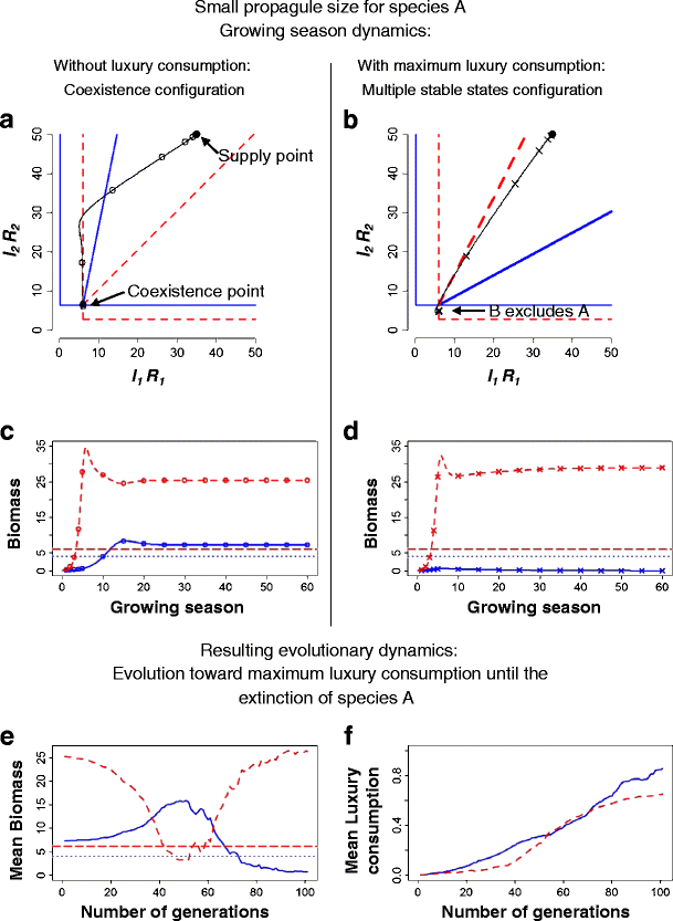
Illustration of the competitive dynamics with and without luxury consumption, and resulting evolutionary dynamics of luxury consumption, where luxury consumption fosters multiple stable states. a and b Resource depletion during the growing season, without (a, line with open circles) and with maximum (b, line with crosses) luxury consumption, from the supply point (black full circle) to either the coexistence point at the intersection of the ZNGIs (without luxury consumption, a) or to extinction of species A with luxury consumption (b). c and d Growth of species A (solid line) in competition against species B (dashed line) through the growing season. The two competing individuals either have no luxury consumption (c) or are both at maximum luxury consumption (d). Species reproductive thresholds are indicated by the horizontal dotted line (species A) and the horizontal dashed line (species B). In competition runs without luxury consumption, the two species coexist and can reproduce (outcome coexistence in Table 3), whereas in competition runs with maximum luxury consumption, one of the species goes extinct, depending on relative initial advantage conferred by their relative propagule size (in this case species A goes extinct, outcome X lux = A in Table 3). We predict coexistence without luxury consumption, and evolution of luxury consumption until species A goes extinct (Table 3). e–f Evolutionary dynamics of luxury consumption follow the predicted outcomes. e Mean biomass and reproductive threshold (horizontal lines) through evolutionary time. Variation in individuals’ luxury consumption strategies allows some individuals to reproduce when mean biomass is below reproductive threshold. f Mean values of luxury consumption evolve towards higher values until species A goes extinct. Other model parameters are I 1 = 35, I 2 = 50, l 1 = 0.6, l 2 = 0.3, m A = 0.5, m B = 1, u A1 = 6, u A2 = 6, u B1 = 3, u B2 = 7, K A1 = 3, K A2 = 30, K B1 = 20, K B2 = 55, a A = 5, a B = 1. In this figure, species A has a small propagule size: p A = 0.05; a case with a larger propagule size is illustrated in the Electronic supplementary material, Fig. B2
-
-
3.
Competitive outcomes with and without luxury consumption.
The evolutionary dynamics of luxury consumption can usually be inferred from the outcomes of within-season competition dynamics where competitors lack luxury consumption and as well as where they have maximum luxury consumption. Competitive outcome may vary, however, depending on propagule biomass and the length of the growth season.
For a long growing season, population dynamics have time to reach equilibrium (Fig. 2c, d). As a result, initial propagule size does not affect the competitive outcome except for cases in which there are multiple stable states (as in Fig. 2b, d). In the case of multiple stable states, some combinations of relative propagule sizes tip the outcome towards one or the other monoculture. For a shorter growing season, transient dynamics become important, and can lead to non-equilibrium outcomes (Electronic supplementary material section C).
-
4.
Evolutionary dynamics of luxury consumption.
Under local competition for resources, we expect luxury consumption to have a selective advantage so long as the two strategies compete. This is because under the vast majority of conditions, higher fitness is achieved with higher luxury consumption of a target individual in interspecific competition. Preemption of the non-limiting resource through luxury consumption decreases the growth of the competitor, limiting the competitive impact of the competitor on the target individual. If one species goes extinct, then luxury consumption becomes a neutral trait for the remaining species. Thus, knowledge of what happens with maximum, or without luxury consumption enables us to predict what happens under evolutionary dynamics: so long as there is coexistence, there is directional selection towards higher luxury consumption, until either both species coexist with maximum luxury consumption, or one goes extinct and the other’s luxury consumption trait becomes neutral (Table 3, Fig. 2, Electronic supplementary material, section B).
We tested the prediction that luxury consumption has a selected advantage using 593 simulations with parameter sets selected as explained in the “Model methods” (Table 3). Each of these 593 non-trivial model parameter sets was run four times in a two-way cross of growing season length (short and long) and initial luxury consumption conditions (none and all strategy combinations). We only present results for long growing seasons in the main text, and results for short growing seasons are presented in Electronic supplementary material, section C.
With a long growing season, we found that the predicted outcome was realized in 97% of all cases, including about 90% of the model runs where we predict selection to favor the evolution towards maximum luxury consumption (between 56 and 58 of 63 cases, depending on initial conditions, see Table 3). Exceptions to the predicted cases were of three general types: (1) extinction of the species other than that predicted (n = 4 across the two sets of initial conditions); (2) evolution of maximum luxury consumption and coexistence when extinction of one of the competitors was predicted (n = 16); or (3) the simulation timed out after 10,000 generations when maximum luxury consumption was predicted (n = 12).
The first two types of exceptions are explained by stochastically generated variation in the luxury consumption trait that may enable one of the species to exceed its reproduction threshold and persist despite being predicted to go extinct. In this case, there is more coexistence than predicted as a consequence of luxury consumption. In the third type of exceptions, luxury consumption evolution can fail to evolve despite being predicted. This can happen when luxury consumption is weakly selected for, neutral or even counter-selected. Luxury consumption was a completely neutral trait in two instances out of the 593 × 2 species cases explored; it was counter-selected in one instance, where luxury consumption resulted in fast depletion dynamics and species’ extinction during the transient phase.

Discussion
Introducing the potential for luxury resource consumption into a classic resource competition model significantly reduces the potential for species coexistence. Luxury consumption of a non-limiting resource has the effect of reducing the availability of that resource for competing species. When this resource is limiting for the competitor, such change can lead to the competitive exclusion of the competitor. By relaxing what empirically appears to be an unrealistic assumption of the classic resource ratio models and allowing uptake of resources that exceed those applied immediately to growth, we find that the zone of coexistence between organisms is greatly reduced. The specific outcome of a competitive interaction in a system that allows luxury consumption of resources depends on the ability of each species to consume excess resources, the limiting resource isoclines of each species and the resource supply point (Fig. 1). This conclusion is particularly important given the ubiquity of empirical observations of luxury consumption of nutrient resources (e.g., Chapin et al. 1990; Stevenson and Stoermer 1982; Tripler et al. 2002).
Empirical studies of luxury consumption have generally regarded the garnering of excess resources to be a bet hedging strategy against potential future shortage (Chapin et al. 1990). A variety of environmental factors, such as pulsed nutrient supplies, may thus result in selection favoring luxury consumption as a strategy for hoarding resources for future use.
The model we present here supports the hypothesis that natural selection can also favor luxury consumption by providing a competitive advantage under common ecological conditions. This observation supports the contention that luxury consumption can be a competitive strategy and not simply a risk aversion strategy. Our model shows that under conditions that enable coexistence of individuals of two species competing locally for resources, natural selection will favor luxury consumption. Evolution of luxury consumption often results in the extinction of one of two species, but can sometimes lead to a stable coexistence of the two species with maximum luxury consumption. Under the vast majority of circumstances, no intermediate level of luxury consumption outperforms maximum luxury consumption (one exception out of 1,186 cases). Furthermore, our simulations show that if luxury consumption is an available trait (e.g., selectively advantaged as a bet hedging strategy against temporally varying resource supply), then competitive interactions can foster and abet the evolution of luxury consumption traits.
Our selection model results demonstrate the conditions under which we might expect the evolution of luxury consumption as a competitive strategy: (a) individuals of two species are competing locally for limiting resources; (b) their coexistence is made possible by trade-offs between species such that the limiting resources are different for the two species and each consumes more of the resource that is limiting for them; and (c) the competitive environment stays the same over a sufficient period of time that allows selection to act. Empirical observations of luxury consumption interpret this trait as conferring individual benefit independent of competition (i.e., acquiring resources for later use when the resource maybe in short supply). Thus, there are likely conditions beyond competition that would also favor selection of luxury consumption of resources.
Ecological conditions external to the model described here may preclude luxury consumption from being favored in nature. Nutrient acquisition costs or nutrient storage costs could conceivably offset advantages gained by luxury consumption. However, the growing empirical evidence of the widespread nature of luxury consumption suggests that constraints to luxury consumption are not generally prohibitive and suggest the need for ecological theory to explain the varied reasons why luxury consumption maybe advantageous.
Because of its potentially strong competitive effect, luxury consumption in one species could introduce selection pressure on the competitor species it affects. For example, increased dispersal or dormancy could be expected in a species strongly affected by a luxury-consuming competitor. Theoretical models demonstrate that increased spatial and temporal variance in conditions between patches selects for increased dispersal (Levin et al. 2003). The evolution of luxury consumption in one species could increase spatio-temporal variance in conditions between patches for their competitor species, and therefore select for increased dispersal and or dormancy in this competitor. Furthermore, condition-dependent dispersal and dormancy could be triggered by adverse environmental conditions (Levin et al. 2003) and therefore by the presence of a fierce luxury-consuming competitor.
In conclusion, our results suggest two novel insights. Firstly, there is a reduced likelihood of two-species equilibrium coexistence under competition as a consequence of advantages conferred by luxury consumption of resources. This result is important because the stable two-species coexistence model suggests that within a finely partitioned environment, there maybe many pairwise combinations of multiple species coexistence, thus providing a theoretical framework for understanding the maintenance of biodiversity within an equilibrium context. Our results suggest that this window of opportunity for coexistence maybe far narrower than these previous models suggest. Second, our models suggest an alternative explanation for the empirical observations of luxury resource consumption. Not only might this luxury consumption be a bet hedging strategy for resource use, but it may also confer a competitive advantage that is likely to be favored by natural selection. Given the frequency with which luxury consumption of resources is observed in nature, the results of our model suggest a need to incorporate luxury resource consumption explicitly into assessments of competition and coexistence.
References
Agrawal AA et al (2007) Filling key gaps in population and community ecology. Front Ecol Environ 5:145–152
Boivin JR, Salifu KF, Timmer VR (2004) Late-season fertilization of Picea mariana seedlings: intensive loading and outplanting response on greenhouse bioassays. Ann Forest Sci 61:737–745
Chapin FS (1980) The mineral-nutrition of wild plants. Annu Rev Ecol Syst 11:233–260
Chapin FS III, Schulze E-D, Mooney HA (1990) The ecology and economics of storage in plants. Annu Rev Ecol Syst 21:423–447
Daufresne T, Loreau M (2001) Ecological stoichiometry, indirect interactions between primary producers and decomposers, and the persistence of ecosystems. Ecology 82:3069–3082
DeAngelis DL (1992) Dynamics of nutrient cycling and food webs. Chapman & Hall, London
Doebeli M, Knowlton N (1998) The evolution of interspecific mutualisms. Proc Natl Acad Sci USA 95:8676–8680
Droop MR (1973) Some thoughts on nutrient limitation in algae. J Phycol 9:264–272
Droop MR (1974) Nutrient status of algal cells in continuous culture. J Mar Biol Assoc UK 54:825–855
Droop MR (1983) 25 years of algal growth-kinetics—a personal view. Bot Mar 26:99–112
Ducobu H, Huisman J, Jonker RR, Mur LR (1998) Competition between a prochlorophyte and a cyanobacterium under various phosphorus regimes: Comparison with the Droop model. J Phycol 34:467–476
Elrifi IR, Turpin DH (1985) Steady-state luxury consumption and the concept of optimum nutrient ratios - a study with phosphate and nitrate limited selenastrum-minutum (Chlorophyta). J Phycol 21:592–602
Grover JP (1991a) Dynamics of competition among microalgae in variable environments—experimental tests of alternative models. Oikos 62:231–243
Grover JP (1991b) Resource competition in a variable environment—phytoplankton growing according to the variable-internal-stores model. Am Nat 138:811–835
Grover JP (1997) Resource competition. Chapman & Hall, London
Houle G, Valery S (2003) A mixed strategy in the annual endemic Aster laurentianus (Asteraceae)—a stress-tolerant, yet opportunistic species. Am J Bot 90:278–283
Klausmeier CA, Litchman E, Daufresne T, Levin SA (2004a) Optimal nitrogen-to-phosphorus stoichiometry of phytoplankton. Nature 429:171–174
Klausmeier CA, Litchman E, Levin SA (2004b) Phytoplankton growth and stoichiometry under multiple nutrient limitation. Limnol Oceanogr 49:1463–1470
Klausmeier CA, Litchman E, Levin SA (2007) A model of flexible uptake of two essential resources. J Theor Biol 246:278–289
Koide RT (1991) Nutrient supply, nutrient demand and plant-response to mycorrhizal infection. New Phytol 117:365–386
Lawrence D (2001) Nitrogen and phosphorus enhance growth and luxury consumption of four secondary forest tree species in Borneo. J Trop Ecol 17:859–869
Levin SA, Muller-Landau HC, Nathan R, Chave J (2003) The ecology and evolution of seed dispersal: a theoretical perspective. Annu Rev Ecol Evol Systemat 34:575–604
Li BT, Smith HL (2007) Global dynamics of microbial competition for two resources with internal storage. J Math Biol 55:481–515
Lipson DA, Bowman WD, Monson RK (1996) Luxury uptake and storage of nitrogen in the rhizomatous alpine herb, Bistorta bistortoides. Ecology 77:1277–1285
Miller TE et al (2005) A critical review of twenty years’ use of the resource-ratio theory. Am Nat 165:439–448
Monod J (1950) La technique de culture continue theorie et applications. Ann Institut Pasteur 79:390–410
Murrell DJ, Law R (2003) Heteromyopia and the spatial coexistence of similar competitors. Ecol Lett 6:48–59
Neuhauser C, Pacala SW (1999) An explicitly spatial version of the Lotka-Volterra model with interspecific competition. Ann Appl Probab 9:1226–1259
Pacala SW (1997) Spatial segregation hypothesis. In: Crawley MJ (ed) Plant ecology, 2nd edn. Blackwell Science Ltd, Oxford, pp 546–555
Revilla T, Weissing FJ (2008) Nonequilibrium coexistence in a competition model with nutrient storage. Ecology 89:865–877
Silvertown J (2004) Plant coexistence and the niche. Trends Ecol Evol 19:605–611
Smith HL, Waltman P (1994) Competition for a single limiting resource in continuous-culture—the variable-yield model. SIAM J Appl Math 54:1113–1131
Sommer U (1991) A comparison of the Droop and the Monod Models of nutrient limited growth applied to natural-populations of phytoplankton. Funct Ecol 5:535–544
Sommer U (2002) Competition and coexistence in plankton communities. In: Sommer U, Worm B (eds) Competition and coexistence, vol 161. Sprinter, Berlin
Sterner RW, Elser J (2002) Ecological stoichiometry: the biology of elements from molecules to the biosphere. Princeton University Press, Princeton
Sterner RW, Schwalbach MS (2001) Diel integration of food quality by Daphnia: Luxury consumption by a freshwater planktonic herbivore. Limnol Oceanogr 46:410–416
Stevenson RJ, Stoermer EF (1982) Luxury consumption of phosphorus by benthic algae. Bioscience 32:682–683
Tilman D (1977) Resource competition between planktonic algae—experimental and theoretical approach. Ecology 58:338–348
Tilman D (1982) Resource competition and community structure. Princeton University Press, Princeton
Tilman D (1988) Plant strategies and the dynamics and structure of plant communities. Princeton University Press, Princeton
Tilman D (1994) Competition and biodiversity in spatially structured habitats. Ecology 75:2–16
Travis JMJ, Brooker RW, Clark EJ, Dytham C (2006) The distribution of positive and negative species interactions across environmental gradients on a dual-lattice model. J Theor Biol 241:896–902
Trent JD, Svejcar AJ, Bethlenfalvay GJ (1993) Growth and nutrition of combinations of native and introduced plants and mycorrhizal fungi in a semiarid range. Agric Ecosyst Environ 45:13–23
Tripler CE, Canham CD, Inouye RS, Schnurr JL (2002) Soil nitrogen availability, plant luxury consumption, and herbivory by white-tailed deer. Oecologia 133:517–524
Turpin DH (1988a) Physiological mechanisms in phytoplankton resource competition. In: Sandgren C (ed) Growth and reproductive strategies of freshwater phytoplankton. Cambridge University Press, New York, pp 316–368
Turpin DH (1988b) Physiological mechanisms in phytoplankton resource competition. In: Sandgren C (ed) Growth and reproductive strategies of freshwater phytoplankton. Cambridge University Press, New York, pp 316–368
van Wijk MT, Williams M, Gough L, Hobbie SE, Shaver GR (2003) Luxury consumption of soil nutrients: a possible competitive strategy in above-ground and below-ground biomass allocation and root morphology for slow-growing arctic vegetation? J Ecol 91:664–676
Yamamura N, Higashi M, Behera N, Wakano JY (2004) Evolution of mutualism through spatial effects. J Theor Biol 226:421–428
Acknowledgement
We thank the NERC Centre for Population Biology at Silwood Park for providing funds to initiate this collaborative effort. David Turpin, James Grover and three anonymous reviewers provided helpful comments on previous versions of the manuscript. Claire de Mazancourt acknowledges a Discovery grant from the Natural Sciences and Engineering Council of Canada. Computational resources were provided by CLUMEQ Super Computing Centre (http://www.clumeq.ca).
Open Access
This article is distributed under the terms of the Creative Commons Attribution Noncommercial License which permits any noncommercial use, distribution, and reproduction in any medium, provided the original author(s) and source are credited.
Author information
Authors and Affiliations
Corresponding author
Electronic supplementary material
Below is the link to the electronic supplementary material.
ESM 1
(DOC 35.7 kb)
Fig. B1
Six possible configurations of ZNGI and resource ratios vectors and their resulting combinations of the nine possible evolutionary outcomes as indicated by shading regions (see text). (PDF 307 kb)
Fig. B2
This figure is the same as Fig. 2 in the main manuscript, with the only difference that species A has a larger propagule size, pA = 0.5. This reverses the outcome of competition with luxury consumption and enables species A to outcompete species B through the evolution of luxury consumption. (PDF 307 kb)
Fig. C1
Effect of the growing season length on competitive outcome and evolutionary dynamics of luxury consumption. All graphs are as in Figure 2. (a,b): Resource depletion during the growing season competitive dynamics without (panel a, open circles) and with maximum (panel b, crosses) luxury consumption. (c,d) Growth of species A (solid line) in competition against species B (dashed line) depending on the length of the growing season, with no luxury consumption (c) and with maximum luxury consumption (d). Two growing season lengths (vertical thin lines, 18 days and 60 days) result in different competitive outcomes with maximum luxury consumption (panel d): coexistence for a short growing season, and extinction of species B for a long growing season. Without luxury consumption, the competitive outcome is coexistence (panel c). From the competitive outcomes we predict the following evolutionary outcomes: evolution towards maximum luxury consumption and coexistence for a short growing season (panels e-f), and evolution toward maximum luxury consumption until extinction of B for a long growing season. (panels g-h) Evolutionary dynamics of luxury consumption follow the predicted outcomes. Other model parameters are I1 = 20, I2 = 60, l1 = 0.7, l2 = 0.7, mA = 1.3, mB = 1.4, uA1 = 10, uA2 = 10, uB1 = 7, uB2 = 10, KA1 = 30, KA2 = 30, KB1 = 50, KB2 = 65, aA = 4, aB = 2. (PDF 307 kb)
Rights and permissions
Open Access This is an open access article distributed under the terms of the Creative Commons Attribution Noncommercial License (https://creativecommons.org/licenses/by-nc/2.0), which permits any noncommercial use, distribution, and reproduction in any medium, provided the original author(s) and source are credited.
About this article
Cite this article
de Mazancourt, C., Schwartz, M.W. Starve a competitor: evolution of luxury consumption as a competitive strategy. Theor Ecol 5, 37–49 (2012). https://doi.org/10.1007/s12080-010-0094-9
Received:
Accepted:
Published:
Issue Date:
DOI: https://doi.org/10.1007/s12080-010-0094-9