Policy drivers for improving electricity end-use efficiency in the USA: an economic–engineering analysis

Abstract

This paper estimates the economically achievable potential for improving electricity end-use efficiency in the USA from a sample of policies. The approach involves identifying a series of energy efficiency policies tackling market failures and then examining their impacts and cost-effectiveness using Georgia Institute of Technology's version of the National Energy Modeling System. By estimating the policy-driven electricity savings and the associated levelized costs, a policy supply curve for electricity efficiency is produced. Each policy is evaluated individually and in an integrated policy scenario to examine policy dynamics. The integrated policy scenario demonstrates significant achievable potential: 261 TWh (6.5 %) of electricity savings in 2020 and 457 TWh (10.2 %) in 2035. All 11 policies examined were estimated to have lower levelized costs than the average electricity retail price. Levelized costs range from 0.5 to 8.1 cents/kWh, with the regulatory and information policies tending to be most cost-effective. Policy impacts on the power sector, carbon dioxide emissions, and energy intensity are also estimated to be significant.

Appendix: GT-NEMS modeling and cost estimations of energy efficiency policies

A portfolio of 11 policies was modeled with GT-NEMS to assess the achievable potential of electricity efficiency. NEMS outputs from individual policy scenarios were used in supplemental spreadsheet analysis to calculate the LCOE saved. This appendix provides information about modeling details and cost estimations policy by policy.

• 1. Appliance incentives offer a 30 % subsidy to reduce the capital cost for the most efficient technologies in residential buildings based on the GT-NEMS technology menu. This amount of subsidy is chosen because many state and federal programs offer financial incentives of 30 % for clean energy investments. For instance, the American Taxpayer Relief Act of 2012 renewed the residential energy efficiency tax credit through December 31, 2013. Its credit ranges from about 10 to 30 % for various envelope retrofits and equipment upgrades, including, for example, $300 for a heat pump water heater or a 90 % efficient gas water heater. The State Energy-Efficient Appliance Rebate Program offered similar levels of subsidies for appliances from 2009 to 2011. In 2008, the American Recovery and Reinvestment Act created a 30 % ITC for solar energy. The Energy Policy Act of 2005 established a tax credit for commercial and residential PV and solar hot water heaters of 30 %, up to $2,000 per home. For this reason, the other two financial incentives in this analysis, the commercial financing policy and the CHP incentives policy, apply the same amount of subsidies to reduce the capital costs of energy-efficient technologies.

  A list of 25 selected technologies from the major end-uses eligible for incentives can be found in Table 10. A subsidy was provided to these technologies to reduce their capital costs by 30 % in this policy scenario.

  Table 10 Most efficient home appliances and equipment

  The appliance incentives policy would incur two types of costs. The private investment which is the expenditure spent by residential consumers to purchase equipment. Table 11 shows the difference in equipment expenditure between the policy case and the reference. The negative private costs suggest that the subsidy can offset the incremental cost of purchasing energy-efficient equipment. The cost burden is borne by the program with over $3 billion every year spent by the public sector to provide subsidy. The total cost of the policy is the sum of both the private and public costs, and it is estimated to be $2.9 billion in 2035. By weighting the cost with electricity savings, the LCOE is estimated at 6.7–8.0 cents/kWh (Table 11).

  Table 11 Cost estimations from appliance incentives

• 2. In the residential building energy codes case, four new codes were added to the building codes profile to force shell efficiency improvements. These codes were modeled with relatively high heating and cooling shell efficiency and relatively high shell installation costs in the attempt to mimic the periodic code updates.

  In the reference case, new residential buildings are built either to no code or in compliance with four different levels of codes: IECC 2006, Energy Star, Forty (40 % above IECC 2006 code), and PATH (50 % above IECC 2006) codes. We constructed a policy scenario where existing building codes are replaced by new codes to ensure efficiency improvements roughly 5 % every 5 years. The building codes scenario was set up based on EIA's Expanded Standards and Codes side case (EIA, 2012), where four new codes were added including “IECC 2006+” (about 30 % above IECC 2006), “IECC 2006++” (about 5 % above IECC 2006+), “IECC 2006+++” (about 5 % above IECC 2006++), and “New Code” (about 5 % above IECC 2006+++) to mimic gradual code improvements. Each newly added code has higher cost associated with efficiency improvements. Table 12 shows the modeling details about residential building codes.

  Table 12 Building energy codes profile for residential buildings

  The policy case also accounts for regional differences in code adoption (Fig. 8). For example, the Pacific division is the early adopter of the IECC 2006, Energy Star, Forty, and IECC 2006+ codes, while the East South Central division is the most lagged adopter of these codes. Energy Star, Forty, and IECC 2006+ retire 5 years later than IECC 2006 with time variance among census divisions. But the IECC 2006++ retires at 2023 for all regions; and the IECC 2006+++ code retires at 2028 for all regions. The “New Code” and the PATH code, the two most stringent codes, stay available for all years and all regions.

  Fig. 8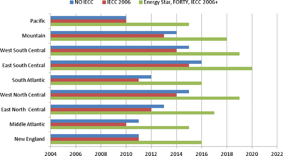

  

  Building energy code retirement years by census division

  New houses built in compliance with new codes consume less energy due to better insulation and building design. Although under new codes installation costs get higher, compliance to the new codes improves over time (Fig. 9).

  Fig. 9

  

  Share of new houses built in the policy case

  The LCOE was calculated based on the difference in private and public costs between the policy scenario and the reference. Cost to the private sector is the incremental cost of equipment plus the installation cost for better building envelopes. By installing more thermally efficient envelopes, HVAC equipment can be downsized due to lower building load requirement. This phenomenon is reflected by the negative private cost, suggesting less money spent on building equipment in the policy case than the reference case (Table 13). To estimate program administrative costs, we assume that cost associated with building code enforcement would be represented by the budget of each state hiring their building code officials and inspectors. The administrative costs are based on each state adding one administrative office run at $150,000 per annum budget and one code official at $75,000 salary per annum. It also includes two additional building code inspectors for the verification of every 100 million ft² in the state at $75,000/year (Brown et al., 2009). The levelized cost is estimated to be 0.5–0.8 cents/kWh (Table 13).

  Table 13 Cost estimations from residential building energy codes

• 3. The on-bill financing program offers zero-interest loans to the most efficient home appliances and equipment. The technologies eligible for zero-interest loans are the same technologies that are eligible for appliance subsidies as listed in Table 10. In GT-NEMS modeling, consumer choice of energy-using equipment is based on life cycle cost. To model on-bill financing, we changed the equations of life cycle cost calculation. In the reference case, the life cycle costs for residential technologies are calculated as following:

  $$ {\mathrm{LFCY}}_{\mathrm{y},\mathrm{es},\mathrm{b},\mathrm{r},\mathrm{v}}={\mathrm{CAPITAL}}_{\mathrm{es}}+{\mathrm{OPCOST}}_{\mathrm{y},\mathrm{es},\mathrm{b},\mathrm{r},\mathrm{v}}\times \left(\frac{1-{\left(1+\mathrm{DIST}\right)}^{-\mathrm{HORIZON}}}{\mathrm{DIST}}\right) $$

  To bring in financing option with variable interest rates and payback periods, we changed the life cycle cost equation to:

  $$ {\mathrm{LFCY}}_{\mathrm{y},\mathrm{es},\mathrm{b},\mathrm{r},\mathrm{v}}=\left({\mathrm{ANNUALPAY}}_{\mathrm{es}}+{\mathrm{OPCOST}}_{\mathrm{y},\mathrm{es},\mathrm{b},\mathrm{r},\mathrm{v}}\right)\times \left(\frac{1-{\left(1+\mathrm{DIST}\right)}^{-\mathrm{HORIZON}}}{\mathrm{DIST}}\right) $$

  When interest rate is 0 %, we have:

  $$ \mathrm{ANNUALPAY}=\frac{\mathrm{CAPITOL}}{\mathrm{CAPHOR}} $$

  When interest rate is >0 %, we have:

  $$ \mathrm{ANNUALPAY}=\mathrm{CAPITOL}\times \frac{\mathrm{CAPDISRT}}{1-{\left(1+\mathrm{CAPDISRT}\right)}^{-\mathrm{CAPHOR}}} $$

  where LFCYCLE is the life cycle costs by equipment class, building type, and census division; CAPITAL is the capital costs for appliances; OPCOST is the operational costs for appliances; DIST is the discount rate for the operational cost during the lifetime of the appliances; HORIZON is the appliance lifetime; ANNUALPAY is the annual payment for on-bill financing equipment; CAPHOR is payback time; and CAPDIST is the interest rate offered by the on-bill financing program.

  In the policy scenario, the 25 selected technologies were assigned a 0 % interest rate and 10-year payback time. Other technologies were assigned nonzero interest rate, indicating their life cycle costs were calculated with the original equation.

  With on-bill financing, increased private investment is the increased expenditure for purchasing home appliances and equipment. Loan cost is the initial seed money put into the program for zero-interest loans. Program administrative cost is estimated as $0.13/MMBtu energy saved. The LCOE associated with on-bill financing is estimated to be 6.6–7.4 cents/kWh (Table 14).

  Table 14 Cost estimations from on-bill financing

• 4. The market priming policy also targets the same set of technologies, as shown in Table 10, but was modeled with hurdle rate changes. Providing information is assumed to lower discount rate when consumers make investment decisions. GT-NEMS modeling of this policy changed the hurdle rates of the efficient technologies to 7 %.

  With market priming, private investment increases when consumers purchase more of the efficient appliances and equipment. Public cost is represented by program administrative cost, estimated as $0.13/MM Btu energy saved. The levelized cost is estimated to be 2.7–3.6 cents/kWh for market priming (Table 15).

  Table 15 Cost estimations from market priming

• 5. The aggressive appliance policy forces retiring the least efficient technologies from the marketplace at 2012. In GT-NEMS, the selected technologies were made either unavailable after 2012 or assigned a hurdle rate equals to 100 %, making these technologies never be chosen to meet energy SD. A list of forced retired technologies is shown in Table 16.

  Table 16 Residential technologies forced early retirement

  Similar to the market priming policy, the cost estimation for the aggressive appliance policy has private cost for the incremental expenditure from equipment purchases and public cost from program administrative costs. The levelized cost is estimated to be 0.6–0.7 cents/kWh (Table 17).

  Table 17 Cost estimations from aggressive appliance policy

  Unlike the residential energy efficiency policies where LCOEs were calculated based on equipment units, cost estimation for commercial policies was based on SD. We estimate the magnitude of technology investment costs in the commercial buildings separately for new purchases, replacements, and retrofits. In each case, the calculation is based on GT-NEMS estimates of SD for energy.

  For new purchases:

  $$ \mathrm{Investment}\ \mathrm{Cost}={\mathrm{SD}}_{\mathrm{new}}\times \left(\mathrm{Cost}/8,760\right)/\mathrm{CF} $$

  where CF is the equipment-specific capacity factor.

  For replacements:

  $$ \mathrm{Investment}\ \mathrm{Cost}={\mathrm{SD}}_{\mathrm{replacement}}\times \left(\mathrm{Cost}/8,760\right)/\mathrm{CF} $$

  For retrofits, we assume the average amount of commercial floor space undergoing a retrofit is 2.2 %. We use the following equation to proportion the surviving SD to the commercial sector retrofit average:

  $$ \begin{array}{l}\mathrm{Investment}\ \mathrm{Cost}={\mathrm{SD}}_{\mathrm{surviving}}\times \left(\mathrm{Cost}/8,760\right)/\mathrm{CF}\times 0.022/\left({\mathrm{SD}}_{\mathrm{surviving}}/{\mathrm{SD}}_{\mathrm{total}}\right)\hfill \\ {}\mathrm{where}\ {\mathrm{SD}}_{\mathrm{total}}={\mathrm{SD}}_{\mathrm{new}}+{\mathrm{SD}}_{\mathrm{replacement}}+{\mathrm{SD}}_{\mathrm{surviving}}\hfill \end{array} $$

• 6. In the benchmarking policy case, GT-NEMS uses a combination of discount rates and the rate for US government 10-year treasury notes to calculate consumer hurdle rates used in making equipment-purchasing decisions. While the macroeconomic module of GT-NEMS determines the rate for 10-year treasury notes endogenously, the discount rates are inputs to the model. Modifying these inputs is the primary means of estimating the impact of benchmarking for the commercial sector in this analysis. This is done in two steps: first, by updating the discount rates to reflect a broader selection of the literature; and second, by adjusting the updated discount rates to account for the effects of a national benchmarking policy.

  To illustrate, Table 18 presents the 2015 hurdle rates used in GT-NEMS across scenarios for two major end-uses in the commercial sector, space heating and lighting (these values represent the sum of the treasury bill rates and the discount rates).

  Table 18 Discount rates across scenarios for space heating and lighting in 2015

  The Benchmarking policy provides energy performance information on commercial buildings. Equipment expenditure increases with this policy. Program administrative cost was estimated as $0.13/MMBtu energy saved. The LCOE is estimated to be 0.9–1.4 cents/kWh (Table 19).

  Table 19 Cost estimations from benchmarking

• 7. The commercial building code is modeled, in part, by assuming a more rapid rate of commercial shell efficiency improvement, as shown in Table 20. Code requirements of efficiency improvements for HVAC equipment is also incorporated in GT-NEMS modeling.

  Table 20 Commercial building shell efficiency improvement

  In this policy scenario, private investment is the incremental cost of equipment and building envelope expenditures to meet new building codes. This policy assumes costs associated with building code enforcement carried out by state building code officials and inspectors. The assumptions about code enforcement cost (the cost of running an administrative office and hiring inspectors) stay the same as in the residential building codes policy. The levelized cost is estimated to be 3.4–4.6 cents/kWh, with most of the cost burden falling on the private sector (Table 21).

  Table 21 Cost estimations from commercial building codes

• 8. In the commercial financing policy case, a 30 % subsidy was provided to 107 technologies, based on a prior analysis of the impact of implementing a carbon tax (Brown et al., 2012). The subsidized technologies are listed in Table 22.

  Table 22 Incentivized technologies in commercial financing policy case

  In the financing case, total cost was estimated to be the sum of increased equipment expenditure (policy caser versus reference), the cost of subsidizing the most efficient technologies, and the program administrative costs. The levelized cost is estimated to be 7.8–8.1 cents/kWh (Table 23).

  Table 23 Cost estimations from commercial financing

• 9. In various industrial processes, systems using motors, such as compressor, pump, and fan systems, are big users of electricity. The motor standard policy describes a scenario where technology advances are mandated for manufactures to produce higher-efficiency motors and lower energy-consuming motor systems with improved system design and the use of variable-frequency drives. To model the impact of such mandate, we assume that new motor systems save 25 % more energy in 2017. For new motors, we assume that there will be 5 % efficiency improvement for small motors (50 hp or lower) and 3 % efficiency improvement for larger motors. The modification was made effective from 2017 when the new standard is introduced.

  Facility owners have to pay the costs of rewinding and replacing failed motors. The cost associated with the new motor standard is the incremental cost in motor expenditures. The private cost listed in Table 24 suggests that more failed motors are replaced with new motors in place of a new motor standard. The public sector pays the program administrative cost, which is much lower than the private cost. The LCOE in this policy case is estimated to be $2.4–3.9cents/kWh (Table 24).

  Table 24 Cost estimations from motor standard

• 10. In the CHP incentives scenario, subsidies were applied to industrial CHP systems to promote efficient usage of waste heat in various industrial processes. A 10-year subsidy increasing from 15 to 30 % was applied to the total installed cost of CHP systems. We assume that, in the CHP market, retailers are able to share the benefits of the subsidy with the consumers at the beginning. All benefits gradually go to the consumers. To reflect this phenomenon, a 15 % subsidy was applied for the first 3 years, rising by 5 % every year from 2015 and staying at 30 % from 2017 to 2021. GT-NEMS represents CHP as a combination of eight technology systems, including two internal combustion CHP systems (ranging from 1 to 3 MW), five gas turbine CHP systems (3 to 40 MW), and one combined cycle system (with two 40-MW gas turbines and a 20-MW steam turbine).

  We account for the increased natural gas consumption and increased equipment expenditure as the private cost associated with the CHP incentives policy. Subsidy cost was estimated based on the amount of incremental cost in CHP investments, while program administrative cost was estimated as 2 % of subsidy cost. The LCOE in this policy case is estimated to be 1.5–2.3 cents/kWh (Table 25).

  Table 25 Cost estimations from CHP incentive

• 11. The plant and technology upgrade policy characterizes the voluntary plant upgrades by the private sector. It took the estimated electricity and natural gas savings from plant utility and technology upgrades reported from 2010 to 2012 in the IAC database (Table 26). The percentage savings were applied to change the TPC parameter in the itech.txt input file.

  The plant and technology upgrade is a combination of R&D and demonstration programs, which aim at identifying the most significant energy-saving opportunities associated with new technologies that can be applied to various industrial processes and sectors. Information is shared among facility owners about energy savings with plant utility upgrades, including non-energy-related upgrades. It is assumed that information and technical assistance is able to stimulate volunteer upgrades in plants and firms. In addition, plant utility can be upgraded for non-energy-saving reasons. For instance, the recent trend of price drop for natural gas may motivate some factories to switch from electronically operated equipment to fossil fuel equipment. This type of upgrades can result in involuntary electricity savings with higher natural gas consumption.

  The GT-NEMS modeling account for policy impacts on both electricity and natural gas. This analysis is unavoidably limited to its data source, while the IAC database has a small sample size with a majority of small-sized and medium-sized firms. The extremely large potentials are likely the result of fuel switching and small sample sizes. In some cases, the large electricity savings are generally coupled with natural gas (or other fuels) penalties. For example, in the chemical industry, an increase of natural gas consumption of 65 % in the West is skewed by one plant in California producing adhesives and sealants. It switched from electronically operated equipment to fossil fuel equipment, resulting in a 200 % increase in natural gas consumption with 60 % savings in electricity. Another instance is the textile industry in the Northeast, where one plant in Massachusetts implemented an upgrade in the time period of investigation. This plant installed cogeneration equipment, which uses a fossil fuel engine, saving 89 % of electricity while using 11 % more natural gas.

  Table 26 Electricity and natural gas saving estimations from IAC reports

  For LCOE calculation, private cost was estimated as the incremental investment for plant upgrades in the private sector (policy case versus reference). Following the division of industrial plants by Brown et al. (2011), this study grouped firms into small-sized, medium-sized, and large-sized firms (Fig. 10). It is assumed that the private investment is $14/MMBtu energy saved for large firms and $12.6/MMBtu energy saved for small and medium firms (Brown et al., 2011).

  Fig. 10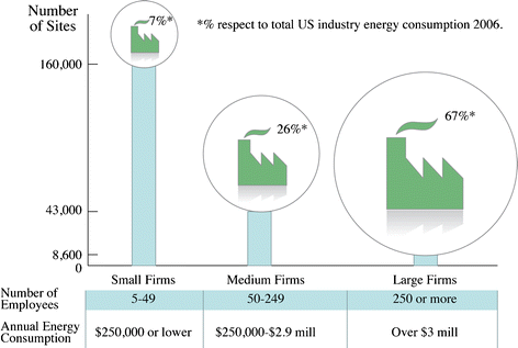

  

  US industrial consumption by size of firm (Brown et al., 2011)

  The levelized cost associated with the plant and technology upgrade is estimated to be 3.0–4.8 cents/kWh, with investment cost decreasing from $1.34 billion in 2020 to $0.94 billion in 2035 (present value; Table 27).

  Table 27 Cost estimations from plant and technology upgrade

References

Allcott, H., & Greenstone, M. (2012). Is there an energy efficiency gap? Journal of Economic Perspectives, 26(1), 3–28.
Amstalden, R. W., Kost, M., Nathani, C., & Imboden, D. M. (2007). Economic potential of energy-efficient retrofitting in the Swiss residential building sector: The effects of policy instruments and energy price expectations. Energy Policy, 35(3), 1819–1829. Retrieved from http://www.sciencedirect.com/science/article/pii/S0301421506002576.
Arimura, T. H., Newell, R. G., Medina, Z., Iwata, K., Myers, E., Mi, J., Jacobsen, M. (2011). Cost-effectiveness of electricity energy efficiency programs. Cambridge: NBER.
Auffhammer, M., Blumstein, C., & Fowlie, M. (2008). Demand side management and energy efficiency revisited. The Energy Journal, 29(3), 91–104.
Azevedo, L., Morgan, M. G., Palmer, K., & Lave, L. B. (2013). Reducing U.S. residential energy use and CO2 emissions: How much, how soon, and at what cost? Environmental Science & Technology, 47, 2502–2511.
Brown, M. A., & Chandler, S. J. (2008). Governing confusion: How statutes, fiscal policy, and regulations impede clean energy technologies. Stanford Law and Policy Review, 19(3), 472–509.
Brown, M. A., Cox, M., & Sun, X. (2012). Modeling the impact of a carbon tax on commercial building sector. In Proceedings of the ACEEE Summer Study on Energy Efficiency in Buildings, Pacific Grove, CA.
Brown, M. A., Gumerman, E., Sun, X., Baek, Y., Wang, J., & Cortes, R. (2010). Energy efficiency in the south. Atlanta: Southeast Energy Efficiency Alliance.
Brown, M. A., Jackson, R., Cox, M., Cortes, R., Deitchman, B., & Lapsa, M. V. (2011). Making industry part of the climate solution: Policy options to promote energy efficiency. Tennessee: Oak Ridge.
Brown, M. A., Laitner, J. A., Chandler, S., Kelly, E. D., Vaidyanathan, S., McKinney, V., Langer, T. (2009). Energy efficiency in Appalachia: How much more is available, at what cost, and by when? Retrieved from http://www.arc.gov/research/researchreportdetails.asp?REPORT_ID=70.
Brown, M. A., Levine, M. D., Romm, J. P., Rosenfeld, A. H., & Koomey, J. G. (1998). Engineering–economic studies of energy technologies to reduce greenhouse gas emissions: Opportunities and challenges. Annual Review of Energy and the Enivronment, 23, 287–385.
Brown, M. A., Levine, M. D., Short, W., & Koomey, J. G. (2001). Scenarios for a clean energy future. Energy Policy, 29(14), 1179–1196. doi:10.1016/S0301-4215(01)00066-0.
Brown, M. A., & Sovacool, B. K. (2011). Barriers to the diffusion of climate-friendly technologies. International Journal of Technology Transfer and Commercialization, 10(1), 43–62.
Coller, M., & Williams, M. B. (1999). Eliciting individual discount rates. Experimental Economics, 2(2), 107–127. Retrieved from http://www.library.gatech.edu:2048/login?url=http://search.proquest.com/docview/222808532?accountid=11107.
Committee on Climate Change Science and Technology Integration (CCCSTI). (2009). Strategies for the commercialization and deployment of greenhouse gas intensity-reducing technologies and practices. Washington: CCCSTI.
Cox, M., Brown, M. A., & Sun, X. (2013). Energy benchmarking of commercial buildings: A low-cost pathway toward urban sustainability. Environmental Research Letters, 8(3), 035018. doi:10.1088/1748-9326/8/3/035018.
Croucher, M. (2011). Potential problems and limitations of energy conservation and energy efficiency. Energy Policy, 39(10), 5795–5799. doi:10.1016/j.enpol.2011.07.011.
Dietz, T. (2010). Narrowing the US energy efficiency gap. In Proceedings of the National Academy of Sciences (p. 16007).
Electric Power Research Institute (EPRI). (2009). Assessment of achievable potential from energy efficiency and demand response programs in the U.S. (2010–2030). Palo Alto: EPRI.
Feng, D., Sovacool, B. K., & Minh Vu, K. (2010). The barriers to energy efficiency in China: Assessing household electricity savings and consumer behavior in Liaoning Province. Energy Policy, 38(2), 1202–1209. Retrieved from http://www.sciencedirect.com/science/article/pii/S0301421509008404.
Foster, B., Chittum, A., Hayes, S., Neubauer, M., Nowak, S., Vaidyanathan, S., Jacobson, A. (2012). The 2012 state energy efficiency scorecard. Washington, DC: ACEEE.
Friedrich, K., Eldridge, M., York, D., Witte, P., & Kushler, M. (2009). Saving energy cost-effectively: A national review of the cost of energy saved through utility-sector energy efficiency programs (vol. 20045). Retrieved from http://aceee.org/research-report/u092.
Fuerst, F., & McAllister, P. (2011). Eco-labeling in commercial office markets: Do LEED and Energy Star offices obtain multiple premiums? Ecological Economics, 70(6), 1220–1230. doi:10.1016/j.ecolecon.2011.01.026.
Geller, H. (2002). Energy revolution: Policies for a sustainable future. Washington, DC: Island Press.
Gellings, C., Wikler, G., & Ghosh, D. (2006). Assessment of U.S. electric end-use energy efficiency potential. The Electricity, 19(9), 55–69.
Goett, A. (1983). Household appliance choice: Revision of REEPS behavioral models. Palo Alto: Electric Power Research Institute.
Hirst, E., & Brown, M. (1990). Closing the efficiency gap: Barriers to the efficient use of energy. Resources, Conservation and Recycling, 3(4), 267–281. Retrieved from http://www.sciencedirect.com/science/article/pii/092134499090023W.
International Energy Agency (IEA). (2007). Energy security and climate policy—Assessing interactions. Paris: OECD/IEA.
Jaffe, A. B., & Stavins, R. N. (1994). The energy-efficiency gap what does it mean? Energy Policy, 22(10), 804–810. Retrieved from http://www.sciencedirect.com/science/article/pii/0301421594901384.
Kim, G., Baer, P., & Brown, M. A. (2013). The statewide job generation impacts of expanding industrial CHP. In Proceedings of the ACEEE Summer Study on Energy Efficiency in Industry, Niagara Falls, NY.
Kneifel, J. (2010). Life-cycle carbon and cost analysis of energy efficiency measures in new commercial buildings. Energy and Buildings, 42(3), 333–340. Retrieved from http://www.sciencedirect.com/science/article/pii/S0378778809002254.
Koopmans, C. C., & te Velde, D. W. (2001). Bridging the energy efficiency gap: Using bottom-up information in a top-down energy demand model. Energy Economics, 23(1), 57–75. doi:10.1016/S0140-9883(00)00054-2.
Laitner, J. A. S., Nadel, S., Elliott, R. N., Sachs, H., & Khan, A. S. (2012). The long-term energy efficiency potential: What the evidence suggests. Retrieved from http://www.aceee.org/sites/default/files/publications/researchreports/e121.pdf.
Levine, M. D., Koomey, J. G., McMahon, J. E., Sanstad, A., & Hirst, E. (1995). Energy efficiency policy and market failures. Annual Review of Energy and the Environment, 20, 535–555.
McKinsey & Co. (2009). Unlocking energy efficiency in the U.S. economy. New York: McKinsey & Co.
Meier, A., Rosenfeld, A. H., & Wright, J. (1982). Supply curves of conserved energy for California's residential sector. Energy, 7(4), 347–358. doi:10.1016/0360-5442(82)90094-9.
Nadel, S., Amann, J., Hayes, S., Bin, S., Young, R., Mackres, E., & Watson, S. (2013). An introduction to U.S. policies to improve building efficiency. Washington, DC: ACEEE.
Nadel, S., Shipley, A., & Elliott, R. N. (2004). The technical, economic and achievable potential for energy-efficiency in the U.S. A meta-analysis of recent studies analysis of recent studies. In 2004 ACEEE Summer Study on Energy Efficiency in Buildings.
National Academies. (2009). Real prospects for energy efficiency in the United States. Washington, DC: The National Academies Press.
Navigant Consulting, Inc. (2013). Assessment of resources within the eastern interconnection. Burlington: Navigant Consulting, Inc.
Office of Management and Budget (OMB). (2002). Guidelines and discount rates for benefit cost analysis of federal programs. Retrieved from http://www.whitehouse.gov/omb/rewrite/circulars/a094/a094.html.
Office of Management and Budget (OMB). (2003). Circular A-4. Retrieved from http://www.whitehouse.gov/sites/default/files/omb/assets/regulatory_matters_pdf/a-4.pdf.
Office of Management and Budget (OMB). (2009). 2010 discount rates for OMB circular no. A-94. Retrieved from http://www.whitehouse.gov/omb/assets/memoranda_2010/m10-07.pdf.
Rogers, E. A., Elliott, R. N., Chittum, A., Bell, C., & Sullivan, T. (2013). Introduction to U.S. policies to improve industrial efficiency, July.
Sadineni, S. B., France, T. M., & Boehm, R. F. (2011). Economic feasibility of energy efficiency measures in residential buildings. Renewable Energy, 36(11), 2925–2931. Retrieved from http://www.sciencedirect.com/science/article/pii/S0960148111001789.
Saygin, D., Patel, M. K., Worrell, E., Tam, C., & Gielen, D. J. (2011). Potential of best practice technology to improve energy efficiency in the global chemical and petrochemical sector. Energy, 36(9), 5779–5790. doi:10.1016/j.energy.2011.05.019.
Scott, M. J., Roop, J. M., Schultz, R. W., Anderson, D. M., & Cort, K. A. (2008). The impact of DOE building technology energy efficiency programs on U.S. employment, income, and investment. Energy Economics, 30(5), 2283–2301. Retrieved from http://www.sciencedirect.com/science/article/pii/S0140988307001119.
Sorrell, S., Dimitropoulos, J., & Sommerville, M. (2009). Empirical estimates of the direct rebound effect: A review. Energy Policy, 37(4), 1356–1371. Retrieved from http://www.sciencedirect.com/science/article/pii/S0301421508007131.
Sreedharan, P. (2013). Recent estimates of energy efficiency potential in the USA. Energy Efficiency, 6(3), 433–445. doi:10.1007/s12053-012-9183-5.
Tonn, B., & Peretz, J. H. (2007). State-level benefits of energy efficiency. Energy Policy, 35(7), 3665–3674. doi:10.1016/j.enpol.2007.01.009.
US Energy Information Administration (EIA). (2009). The national energy modeling system: An overview. Energy (vol. 0581).
US Energy Information Administration (EIA). (2012). Annual energy review 2011 (p. 220).
US Energy Information Administration (EIA). (2013a). Annual energy outlook. Washington, DC: US EIA.
US Energy Information Administration (EIA). (2013b). Interconnection exchange. Retrieved August 5, 2013, from http://www.eia.gov/electricity/wholesale/.
US Environmental Protection Agency (EPA). (2010). Technical support document: Social cost of carbon for regulatory impact analysis under executive order 12866. Retrieved from http://www.epa.gov/otaq/climate/regulations/scc-tsd.pdf.
Zheng, S., Wu, J., Kahn, M. E., & Deng, Y. (2012). The nascent market for “green” real estate in Beijing. European Economic Review, 56(5), 974–984. doi:10.1016/j.euroecorev.2012.02.012.
Author information
Authors and Affiliations
Corresponding author