Wind-Turbine Gear-Box Roller-Bearing Premature-Failure Caused by Grain-Boundary Hydrogen Embrittlement: A Multi-physics Computational Investigation

Abstract

To help overcome the problem of horizontal-axis wind-turbine (HAWT) gear-box roller-bearing premature-failure, the root causes of this failure are currently being investigated using mainly laboratory and field-test experimental approaches. In the present work, an attempt is made to develop complementary computational methods and tools which can provide additional insight into the problem at hand (and do so with a substantially shorter turn-around time). Toward that end, a multi-physics computational framework has been developed which combines: (a) quantum-mechanical calculations of the grain-boundary hydrogen-embrittlement phenomenon and hydrogen bulk/grain-boundary diffusion (the two phenomena currently believed to be the main contributors to the roller-bearing premature-failure); (b) atomic-scale kinetic Monte Carlo-based calculations of the hydrogen-induced embrittling effect ahead of the advancing crack-tip; and (c) a finite-element analysis of the damage progression in, and the final failure of a prototypical HAWT gear-box roller-bearing inner raceway. Within this approach, the key quantities which must be calculated using each computational methodology are identified, as well as the quantities which must be exchanged between different computational analyses. The work demonstrates that the application of the present multi-physics computational framework enables prediction of the expected life of the most failure-prone HAWT gear-box bearing elements.

Introduction

Wind-turbine gear-box failure remains one of the major problems to the wind-energy industry (Ref 1-3). The combination of these high failure rates, long down times, and the high cost of gear-box repair has contributed to: (a) increased cost of wind energy; (b) increased sales price of wind-turbines due to higher warranty premiums; and (c) a higher cost of ownership due to the need for funds to cover repair after warranty expiration. To bring the wind-energy cost down, durability and reliability of gear-boxes have to be substantially improved. These goals are currently being pursued using mainly laboratory and field-test experimental approaches. While these empirical approaches are valuable in identifying shortcomings in the current design of the gear-boxes and the main phenomena and processes responsible for the premature failure of wind-turbine gear-boxes, advanced computational engineering methods, and tools can not only complement these approaches but also provide additional insight into the problem at hand (and do so in a relatively short time). The present work demonstrates the use of these methods and tools, and discusses the benefits offered by them within the context of horizontal-axis wind-turbine (HAWT) gear-box roller-bearing premature-failure.

A photograph of an offshore wind turbine is provided in Fig. 1. All major components of the turbine are labeled for identification. Examination of this figure shows that the HAWT rotor (typically consisting of three blades) attached to a horizontal hub (which is connected to the rotor of the electrical generator, via a gear-box/drive-train system, housed within the nacelle). The rotor/hub/nacelle assembly is placed on a tower, which is in turn anchored to the ocean floor (or ground, in the case of onshore HAWTs).

Fig. 1

A photograph of a typical off-shore wind farm, with the major wind turbine sub-systems identified

Turbine blades and the gear-box (or, in general, the wind-turbine drive-train) are perhaps the most critical components/subsystems in the present designs of wind turbines. The present work deals only with the issues related to the performance, reliability, and modes of failure of gear-box components. In our recent work (Ref 4, 5), the problem of inadequate durability and premature failure of wind-turbine blades was investigated computationally.

The main function of the gear-box is to convert the low speed of the rotor shaft to the high speed of the electrical generator shaft. A labeled schematic of a prototypical wind turbine gear-box is shown in Fig. 2. The low-speed stage of the gear-box is a planetary configuration with either spur (the present case, Fig. 2) or helical gears. In this configuration, the planetary-gear carrier is driven by the wind-turbine rotor, the ring gear is stationary/reactionary, while the sun pinion shaft drives the intermediate gear-box stage, and, in turn, the high-speed stage (the one connected to the rotor of the electric generator). Predominantly, the gear-box failure initiation is observed in planet bearings, intermediate-shaft bearings, and high-speed-shaft bearings (each labeled in Fig. 2).

Fig. 2

Schematic of a prototypical wind-turbine gear-box. The major components and sub-systems are identified. Failure typically occurs within the (planet, intermediate shaft, and high-speed shaft) roller-bearings

In principle, the predicted service-life of properly maintained roller-bearings operating under elasto-hydrodynamic lubrication conditions, and foreseen loading/environmental conditions, is well-predicted using the well-established bearing-reliability assessment procedures (Ref 6-8). The basic assumptions used in these procedures are that the bearing-life is controlled by the material high-cycle fatigue (typically within the bearing races/rings), commonly referred to as the roller-bearing contact fatigue (RCF) failure. The in-service cycling stresses arise from the repeated exposure of the ring material to ring/roller-element non-conformal contact stresses. Under well-lubricated/clean-lubricant conditions, RCF is typically initiated by the nucleation of subsurface cracks (in regions associated with critical combinations of the largest shear stress and the presence of high-potency microstructural defects). During subsequent repeated loading, cracks tend to advance toward the inner surfaces of the raceways, giving rise to the formation of spalls/fragments.

As mentioned earlier, roller-bearings in wind-turbine gear-boxes tend to fail much earlier relative to their expected service life. In addition, the damage mechanism responsible for, and the appearance of roller-bearing prototypical premature-failure seems different from the classic RCF failure. A detailed description of the visual appearance of the standard RCF failure is given in ISO 15243 (Ref 7), and hence will not be repeated here. Instead, a simple schematic of the sub-surface region containing RCF dark and white bands as well as a single chevron-shape crack is depicted in Fig. 3(a). In the case of the premature roller-bearing failure, the damaged region acquires a characteristic “White Etching Crack” appearance, and is initially localized at the contact surfaces or slightly beneath them. This appearance is related to the weak etching response of the associated local microstructure (mainly consisting of equiaxed sub-micron-size carbide-free ferrite grains) during the standard preparation of metallographic samples. In addition to the chevron-shaped cracks like the one shown in Fig. 3(a), so-called butterfly white-etching cracks are also often observed in the case of RCF failure. These cracks are formed at greater depths and are normally associated with excessive loading. In sharp contrast, white-etch cracking in the case of premature roller-bearing failure, Fig. 3(b), is believed to be a surface or near-surface phenomenon (Ref 9). Specifically, it is believed that a combination of disturbed bearing kinematics, unfavorable loading, and inadequate lubrication can lead to local surface or near-surface tensile-stress concentrations, at the root of surface asperities and/or at the near-surface inclusion/matrix interfaces. If these stress concentrations and the number of loading cycles are sufficiently high, surface and/or subsurface cracks can nucleate. Due to proximity of the contact surfaces, subsurface cracks can readily extend to these surfaces (becoming surface cracks).

Fig. 3

Schematics of: (a) the classic rolling-contact fatigue (RCF) fracture/failure; and (b) white-etch cracking (WEC) premature-failure

Cracks nucleated at the contact surfaces are subsequently infiltrated by the lubricant. The lubricant contains various (e.g., extreme pressure, EP, and anti-wear, AW) additives and may be contaminated with water. Passage of the rolling elements over the damaged area can result in hydrodynamic effects, leading to crack spreading, and branching. Newly formed “clean-metal” crack faces tend to readily chemically interact with the lubricant, causing the formation of a chemically altered fracture-toughness-inferior region at the crack tip. These changes, in turn, lead to a transition from a purely mechanical-fatigue-cracking regime to a corrosion-assisted fatigue-cracking regime. The same chemical reactions tend to produce hydrogen, which diffuses into the surrounding crack-tip region, primarily along the grain boundaries. This (embrittling) process reduces grain-boundary cohesion and promotes inter-granular cracking (Ref 9).

In our recent work (Ref 10, 11), the problem of gear-box failure caused by gear-tooth bending-induced fatigue was investigated computationally. However, even when the ultimate failure of the gear-box is localized within the gears, the initial damage which led to this failure could be traced back to one or more gear-box roller-bearings.

In the present work, a multi-physics computational approach is proposed to address the problem of HAWT gear-box roller-bearing premature-failure. While such a computational approach is not a substitute for the re-engineer-and-field-test approach, it can provide complementary insight into the problem of wind-turbine gear-box failure and help gain insight into the nature of the main cause of this failure. In addition, computational engineering analyses enable investigation of the gear-box failure in a relatively short time, under a variety of wind-loading conditions comprising both the expected design-load spectrum as well as the unexpected extreme loading conditions.

Considering the aforementioned potential benefits of the computational analysis, the main objective of the present work is to develop a multi-physics computational framework comprising: (a) quantum-mechanical analysis of grain-boundary hydrogen embrittlement phenomenon and hydrogen-atom jumps along the grain-boundary and through the bulk; (b) atomistic-level kinetic Monte Carlo analysis of hydrogen inter-granular and bulk diffusion and determination of the effective grain-boundary diffusivity; and (c) continuum-type analysis of surface-crack inter-granular spreading and branching assisted by hydrogen-embrittlement and corrosion effects under normal-wind loading conditions which may result in the formation of spalls/fragments within the inner race and, in turn, lead to the bearing-element failure. A flowchart of the multi-physics computational approach used in the present work is shown in Fig. 4.

Fig. 4

A flow-chart showing the multi-length-scale computational analysis, of HAWT-gearbox roller-bearing premature-failure, utilized in the present work. Nomenclature: A—hydrogen diffusion parameters; B—hydrogen embrittlement parameters; C—effective grain-boundary hydrogen diffusivity

A concise summary of the computational approach used in the investigation of wind-turbine gear-box roller-bearing premature-failure and the associated hydrogen-induced grain-boundary embrittlement is presented in section 2. The key results yielded by the present investigation are presented and discussed in section 3, while the main conclusions resulting from the present work are summarized in section 4.

Quantum-Mechanical Analysis of Hydrogen-Induced Grain-Boundary Embrittlement

Premature failure of wind-turbine gear-box roller-bearings is taken to be a manifestation of a hydrogen-induced grain-boundary embrittlement phenomenon. The local extent of hydrogen-induced grain-boundary embrittlement is controlled by two phenomena/processes: (a) the extent of local hydrogen segregation to the grain-boundary; and (b) the extent of grain-boundary normal and tangential strength sensitivity to the local grain-boundary hydrogen concentration. To quantify these phenomena/processes, a series of quantum-mechanical and atomistic-level kinetic Monte Carlo analyses is conducted. The quantum-mechanical calculations, presented in this section, are used to: (a) assess the sensitivity of grain-boundary strength to the local concentration of grain-boundary hydrogen; and (b) to quantify key parameters such as the activation energy and the vibrational frequency associated with the hydrogen diffusion and required in the kinetic Monte Carlo hydrogen-diffusion analysis. Kinetic Monte Carlo simulations, presented in the next section, are used to assess the rate at which hydrogen segregation from the crack-tip/-faces to the adjacent (connected to the crack tip) grain-boundaries takes place.

Problem Formulation

The main problem analyzed in this portion of the work is the extent of grain-boundary hydrogen embrittlement as a function of the degree of hydrogen segregation to the grain-boundary and the structure of the grain-boundary itself. All the calculations carried out in this portion of the work involve the use of the semi-empirical quantum method AM1, as implemented in VAMP computer program (Ref 12).

Computational Modeling and Analysis

Grain-Boundary (GB) Modeling

To construct GBs investigated in the present work, the standard procedure is used which involves: (a) rotation of the two crystals either about an axis residing in the GB plane (for tilt GBs) or an axis normal to the GB plane (for twist GBs); (b) sectioning of the two crystals parallel to the GB plane; and (c) joining the two crystals over the GB plane to form a bicrystal (the computational cell).

Semi-empirical AM1 Method

For the reasons explained in our prior work (Ref 13), the rigorous ab initio quantum mechanical calculations were not used in the present work. Rather, the AM1 method (Ref 14), a computationally efficient semi-empirical quantum mechanical method, is utilized. Within the AM1 method, diatomic differential overlap effects are neglected (i.e., the overlap matrix is replaced with the unit matrix) which enables simplification of the Hartree-Fock secular equation governing the quantum-mechanical behavior of the material system. The AM1 method was chosen because it appears to be the most suitable semi-empirical quantum-mechanical method for the analysis of the hydrogen dissolution in BCC iron (used to represent the conventional bearing steel, within the quantum mechanical framework), since it is parameterized to reproduce experimental results pertaining to hydrogen dissolution energy.

A typical semi-empirical quantum-mechanical calculation involves the following three steps: (a) construction of the material model; (b) application of the quantum-mechanical method; and (c) post-processing analysis and evaluation of the relevant material quantity/quantities.

Results and Discussion

The results presented in Fig. 5 reveal the effect of hydrogen, under the condition of full GB saturation, on the GB normal strength. In this figure, the GB structure varied along the x-axis is represented by the volume of the corresponding interstitial-site Voronoi cells. The results displayed in Fig. 5 reveal that, under the condition of full saturation, the percent decrease in the GB normal strength due to the presence of hydrogen is not a sensitive function of the grain-boundary type. On the other hand, as evidenced by the results also displayed in Fig. 5, the hydrogen-free GB normal strength is a fairly sensitive function of the GB structure. Specifically, as the GB structure becomes more open, as represented by larger Voronoi cells, the hydrogen-free GB normal strength decreases.

Fig. 5

The effect of grain-boundary (GB) structure (as represented by the corresponding interstitial-site Voronoi cell volume) on the GB cohesion strength, and the change in the GB cohesive strength at full saturation with hydrogen

The driving force for hydrogen segregation to the GBs is the hydrogen solution-energy. The lower is this energy, the higher is the tendency of hydrogen to segregate to the GBs. The quantum-mechanical results obtained in the present work pertaining to the effect of grain-boundary structure on the hydrogen solution-energy are depicted in Fig. 6(a). It is seen that as the GB structure becomes more open, the expected extent of hydrogen segregation to the GBs increases. In addition to depending on the GB structure, hydrogen solution-energy is also a function of the distance from the GB. This is exemplified by the results displayed in Fig. 6(b) for the case of the $\varSigma 3\left( {112} \right)\left[ {1\bar{1}0} \right]$ tilt GB. It is seen that as the distance from the GB increases, the hydrogen solution-energy increases (i.e., the expected extent of hydrogen segregation decreases). However, it should be noted that the expected hydrogen segregation to the region adjacent to the grain-boundary is still quite high considering the associated lower solution-energy.

Fig. 6

Dependence of the hydrogen solution-energy on: (a) structure of the grain-boundary (GB) (as represented by the corresponding interstitial-site Voronoi cell volume); and (b) distance from the GB for the case of the $\varSigma 3\left( {112} \right)\left[ {1\bar{1}0} \right]$ tilt GB

The quantum-mechanical calculations carried out in this section provide the critical data for the kinetic Monte Carlo hydrogen diffusion analysis. An example of such data is shown in Fig. 7. In this figure, variation in the computational-cell energy as a function of the hydrogen-diffusion distance in the $\left[ {001} \right]$ direction is shown. Two cases are considered: (a) diffusion through the bulk; and (b) diffusion along the $\varSigma 3\left( {112} \right)\left[ {1\bar{1}0} \right]$ tilt GB. It should be noted that the system-energy range in each case is a measure of the corresponding hydrogen-diffusion activation energy. Examination of the results displayed in Fig. 7 reveals that the bulk-diffusion activation energy is only about 60% of its grain-boundary counterpart. At room temperature, this difference in the diffusion activation energy translates into an approximately 1100-fold increase in the diffusion rate through the bulk relative to that along the grain-boundary. This finding reveals that, while hydrogen has a high tendency to diffuse to the grain-boundaries, hydrogen residing on the grain-boundary has quite low diffusivity along the grain-boundary.

Fig. 7

Variation in the computational-cell energy as a function of the hydrogen-diffusion distance in the $\left[ {001} \right]$ direction for the case of bulk-diffusion and diffusion along the $\varSigma 3\left( {112} \right)\left[ {1\bar{1}0} \right]$ tilt grain-boundary

Atomic-Scale Hydrogen-Diffusion Analysis

The analysis carried out here utilizes the following results yielded by the quantum-mechanical calculations described in the previous section: (i) the number of interstitial-site types; (ii) the coordination of different interstitial-site types; (iii) variation in the system energy along different diffusion paths of the hydrogen atom from the given (occupied) interstitial-site; and (iv) activation energy associated with hydrogen-atom jump from a given (occupied) interstitial site to a neighboring (unoccupied) interstitial-site. It should be noted that only a few selected results yielded by the quantum-mechanical calculations were shown in the previous section, Fig. 6(a), (b), and 7. Many more such results, which were generated (but not shown) in the previous section, are used in this section.

Problem Formulation

The problem analyzed here involves: (a) modeling of hydrogen diffusion from the crack-tip wake region into the adjacent (connected to the crack tip) grain-boundaries; and (b) determination of the effective hydrogen diffusion coefficient. All the calculations carried out utilized atomic-scale kinetic Monte Carlo simulations. To monitor the progress of the hydrogen-diffusion process, hydrogen tracer atoms are introduced (with identical properties as the remaining hydrogen atoms).

Computational Modeling and Analysis

Grain-Boundary (GB) Modeling

Essentially the same geometrical models for the grain boundaries are used in the kinetic Monte Carlo analysis as in the previous quantum-mechanical analysis. Fe-Fe, Fe-H, and H-H interactions are represented using the embedded atom method interatomic potentials (Ref 15). An example of the computational domain used is depicted in Fig. 8(a). In this figure, iron atoms are colored cyan and hydrogen atoms residing on the grain-boundary are colored white, while a single hydrogen tracer atom is colored yellow.

Fig. 8

Kinetic Monte Carlo results for the advancement of the hydrogen front from the crack-tip along the adjoining grain-boundary, showing the (yellow) tracer hydrogen atom: (a) originally in the wake of the crack-tip; (b) and (c) diffusing through the bulk iron adjacent to the grain-boundary; and (d) ultimately arriving at the hydrogen-concentration front along the grain-boundary, causing this front to grow

Kinetic Monte Carlo Method

The temporal evolution of the hydrogen tracer-atom position during the diffusion analysis is simulated using the version of the kinetic Monte Carlo method originally developed by Grujicic and Lai (Ref 16). Within this method, one atomic jump is allowed to take place from one (occupied) interstitial site to the neighboring (unoccupied) interstitial site during each time step. The occurrence of one such jump at one of the (occupied) sites is termed an event. At each time step, a list of all possible events is first constructed, and then the probability for each event is set proportional to the rate at which the associated hydrogen-atom jumps take place. Next, the event to take place is selected randomly. This is accomplished by generating, at each time step, a random number αψ from a uniform distribution function in the (0, 1) range. The value of α is next used to select event m from M possible events in accordance with the procedure described in Ref 9. After an event has occurred, the total number of possible events M is updated and the aforementioned procedure is repeated. The kinetic Monte Carlo method employed in the present work uses a variable time-step to account for the fact that different events require different amounts of time to occur. At each simulation step the time increment is computed using the procedure described in Ref 9. According to this procedure, the maximum time increment allowed is controlled (dynamically and stochastically) by the fastest event(s). Consequently, significant reductions in the computational time are achieved relative to the fixed time-step kinetic Monte Carlo methods.

Results and Discussion

An example of the kinetic Monte Carlo results for the advancement of the hydrogen front from the crack-tip along the adjoining grain-boundary, showing the (yellow) tracer hydrogen atom: (a) originally in the wake of the crack-tip; (b) and (c) diffusing through the bulk iron adjacent to the grain-boundary; and (d) ultimately arriving at the hydrogen-concentration front along the grain-boundary, causing this front to grow, is depicted in Fig. 8(a)-(d). For brevity, other results obtained in this portion of the work will not be presented. Rather, the key findings can be summarized as:

• (a) Diffusion rate of hydrogen along the grain-boundaries is quite small in comparison to its counterpart through the bulk, which is in complete agreement with the quantum-mechanical predictions;

• (b) Once a hydrogen atom has arrived at a grain-boundary, it becomes effectively trapped with very little mobility both in the directions along and normal to the grain-boundary;

• (c) Mass transport of hydrogen from the crack-tip wake region along the adjoining grain-boundaries is effectively controlled not by the grain-boundary diffusion but rather by the diffusion of hydrogen through the adjoining bulk material and its deposition onto the advancing GB-hydrogen front (Ref 17-20);

• (d) While the hydrogen diffusion from the crack-tip through the bulk to the advancing hydrogen-front is associated with a longer diffusion path, the effective hydrogen grain-boundary diffusivity is still controlled by its bulk component. This is the result of two effects: (i) substantially higher bulk diffusivity of hydrogen compared to its inter-granular counterpart; and (ii) the fact that the inter-granular and trans-granular diffusion paths are connected in parallel; and

• (e) Using the procedure described in Ref. 21, the effective (averaged) grain-boundary diffusivity for hydrogen at room temperature has been found to be (1.7 ± 0.1) 10⁻¹¹ m²/s. This value will be used in section 4 to model the progress of hydrogen segregation to the grain-boundaries ahead of the advancing crack-tip.

Roller-Bearing Inner-Race Damage/Failure Analysis

In this section, the problem of surface-crack spreading and branching in the (inner) raceway is analyzed under rolling-element/raceway contact-stresses.

Problem Formulation

The main problem addressed here is the determination of the average time it will take a surface-crack to penetrate deep enough into the raceway, turn around and return to the surface, forming a (potentially failure-causing) spall. It should be noted that the process of nucleation of the surface-crack is not analyzed. Rather, it is assumed that a combination of the unfavorable kinematic conditions within the rolling-element and excessive loading can cause such a crack to nucleate. The time for the surface-crack to propagate as described, when combined with the average time for surface-crack nucleation (not dealt with in the present work) could then serve as an estimate of the roller-bearing predicted life. All simulations in this portion of the work were conducted using ABAQUS/Explicit, a general-purpose finite-element program (Ref 22).

Computational Model and Analysis

Contact-Region Finite-Element Model

To account for the fact that: (a) the rolling-element/raceway contact patch is quite small in comparison to the characteristic dimensions of these components; and (b) the premature failure is frequently found to occur in inner races, the geometrical model analyzed consists of a two-dimensional rectangular region residing fully within the inner race, Fig. 9(a). The roller-element is not modeled explicitly but is rather replaced by the (moving) surface-distribution of the contact-stresses (marked schematically in Fig. 9b) of the type determined in our previous work (Ref 13). To recognize the fact that: (a) surface-crack spreading and branching will be localized near the surface; and (b) crack growth is primarily of the inter-granular character, the upper portion of the computational domain surrounding the previously nucleated crack was assigned a granular structure [using two-dimensional Poisson-type Voronoi cells (Ref 13)]. In this way, common edges of the adjacent Voronoi cells act as (two-dimensional) grain boundaries. The remainder of the computational domain is treated as a featureless, two-dimensional continuum.

Fig. 9

Schematic of diffusion of hydrogen from crack tip through grain boundary and bulk due to lubricant being hydraulically loaded by passage of roller-element

Both the granular and the featureless portions of the computational domain are meshed using a combination of triangular and quadrilateral plane-strain continuum finite elements. In addition, grain boundaries are meshed using four-node traction/separation cohesive-zone elements. These elements enable modeling of the normal- and/or shear-traction induced grain-boundary decohesion (i.e., inter-granular cracking). Furthermore, in order to model hydraulic loading of the partially or fully debonded grain-boundaries, the cohesive-zone elements are assigned additional degrees of freedom (i.e., the pore-pressure). A close-up of the meshed model used in this portion of the work is depicted in Fig. 9(c). It should be noted that, since each cohesive-zone element initially involves two pairs of coincident nodes, they are not (visually) resolved in Fig. 9(c). The mesh typically contains 15,000-20,000 continuum and 4000-5000 cohesive-zone elements.

Analysis of Crack Spreading/Branching Using ABAQUS/Explicit

The finite-element analysis (FEA) employed in this portion of the work requires specification of the following: (a) geometrical model; (b) meshed model; (c) computational algorithm; (d) initial conditions; (e) boundary conditions; (f) contact interactions; (g) material model(s); and (h) computational tool. Details regarding the geometrical and meshed models are presented above. Since the remaining items have been described in our prior work (Ref 13), they will not be repeated here. However, unique features of the FEA used in this portion of the work are presented in the remainder of this section. These include:

• (a) To represent traction-separation constitutive relations for the cohesive-zone elements under hydrogen-/corrosion-assisted inter-granular cracking conditions, a user subroutine had to be created and linked with the ABAQUS solver. The essential feature of these relations is that as the grain-boundary separation increases, the corresponding traction first increases, then reaches a peak and subsequently continues to decrease toward zero (indicating a complete loss of grain-boundary cohesion). Details regarding the functional forms for these constitutive relations are presented in the Appendix. Since the parameters of these functional relationships (e.g., the peak traction, i.e., the cohesive strength) are affected by the extent of hydrogen segregation to the grain-boundaries ahead of the advancing cracks, they were formulated using the results of: (i) a quantum-mechanical analysis revealing the sensitivity of the grain-boundary cohesion strength to the presence of hydrogen (section 2); and (ii) an atomic-level analysis of hydrogen diffusion from the crack-tip wake into the surrounding grain-boundaries (section 3);

• (b) A moving distributed normal-loading (representing rolling-element/inner-race interactions) is applied over the top edge of the computational domain, in a periodic sense. That is, when a portion of the distributed loading leaves the top edge of the computational domain on one side (the right side, in Fig. 9b), an equivalent “missing portion” of the profile contacts the top edge at the other side (the left side, in Fig. 9b). Furthermore, to represent hydrodynamic loading exerted on the crack faces extending to the surface by the infiltrating and pressurized lubricant, a periodic pore-pressure loading function is applied to the “cracked” grain boundaries;

• (c) Inter-granular fracture is modeled as the process of degradation and ultimate failure of the grain-boundary cohesive-zone elements. Once a cohesive-zone finite element is completely degraded/failed, it is removed from the model. Thereafter, the faces of the corresponding elements of the adjacent grains are prevented from interpenetration by activating a penalty-type contact algorithm between them (Ref 23-27); and

• (d) To account for the fact that the evolution portion of the roller-bearing premature-failure process is stress-controlled, the continuum-material (AISI 4340 steel) model is assumed to be of a (isotropic) linearly elastic character.

Prediction of the Bearing-Life Controlled by Inter-granular Cracking

Surface-crack spreading and branching, and thus the associated bearing-life are modeled explicitly in this section. As mentioned above, the rate at which surface-cracks spread/branch and, thus, the bearing-life are controlled by the rate of hydrogen-segregation to the grain-boundaries ahead of the advancing cracks and the extent of grain-boundary cohesive-strength sensitivity to the presence of hydrogen (grain-boundary hydrogen-embrittlement).

To include the effect of grain-boundary hydrogen-embrittlement into the present FEA, the following procedure should be implemented at each computational step:

• (a) since the hydrogen ingress is believed to be diffusion- and not chemical-reaction-controlled (i.e., chemical reactions between the freshly formed crack surfaces and lubricant additives are quite fast), a fixed hydrogen concentration is assumed to exist at the tip of each crack. This concentration corresponds to the condition of hydrogen chemical-potential equality in the lubricant located in the wake of the crack-tip and at the adjacent crack-faces. Then, using the information about the effective grain-boundary diffusivity of hydrogen (as provided by the atomic-scale analysis presented in section 3), the concentration profiles and the associated average concentrations of hydrogen along the (still bonded) grain-boundaries connected to the crack-tip are calculated. To help clarify the procedure implemented in this portion of the work, a simple schematic of a lubricant-filled and hydraulically loaded crack impinging on the two grain-boundaries is depicted in Fig. 10;

  Fig. 10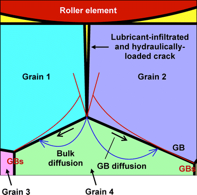

  

  (a) Close-up view of the transverse section of a roller-bearing; (b) geometrical model; and (c) meshed model of the two-dimensional computational domain analyzed

• (b) the information obtained in (a), in conjunction with the sensitivity of the grain-boundary strength to the presence of hydrogen (as provided by the quantum-mechanical analysis, section 2), is used to impart the hydrogen-induced embrittling effect to the grain-boundaries in question. This was done by properly reducing the grain-boundary normal/tangential cohesive-strengths.

• (c) loading induced by the passage of the roller-elements over the computational domain of the raceway is then used within the FEA to further (mechanically) degrade the grain-boundary elements. Two components of this loading are included: (i) surface-type loading associated with the passage of the contact-pressure profile over the top edge of the computational domain; and (ii) hydraulic loading associated with the pressurization of the lubricant, residing within the surface-originating crack(s), due to the passage and the piston-like action of the roller-element over the crack mouth; and

• (d) the progress of a spread-out and branched crack-front is monitored in order to identify the instant when one of the fronts arrives at the raceway free surface. This instant is then identified as the moment of failure of the roller-bearing.

The procedure described above should be applied at each computational step, for the most accurate determination of the initiation and evolution of damage within the computational domain. However, due to a very large number of loading cycles required to produce a spall, a “jump-in-cycles” approach was implemented. This procedure involves the following steps: (i) first, an integer value is assigned to the number of cycles to be skipped, i.e., to the cycle-jump; (ii) the analysis is then performed over a number of consecutive time-steps required to complete one loading cycle, i.e., one passage of the Hertzian contact-pressure over the top edge of the computational domain; (iii) then, the clock is advanced by the time equal to the product of the cycle-jump and the total duration of the just-completed loading cycle; (iv) the time obtained in (iii) is used to update the grain-boundary hydrogen concentration, and the normal and shear cohesive strengths; and (v) the next loading cycle is applied, and the sequence of steps (i)-(v) repeated.

Results and Discussion

In this section, the main results of the finite-element structural analysis, as related to the wind-turbine gear-box roller-bearing premature-failure, and of the associated hydrogen-induced grain-boundary embrittlement, are presented and discussed. While the present computational framework enables the generation of results under various mechanical loading conditions and hydrogen-source conditions in the crack-front wake, only a few prototypical results will be presented and discussed due to space limitations. In our future communication, a more detailed parametric study of the effect of various loading and environmental conditions on the roller-bearing service-life will be presented.

As suggested earlier, premature-failure of wind-turbine gear-box roller-bearings is generally assumed to be initiated by one of the surface-distress processes. Typically, these processes result in the formation of surface cracks. In the present work, it is assumed that the grain subdomain contains, from the onset, two such surface cracks. Using the FEA, it is then investigated how the presence of these cracks and the absence/presence of hydrogen-induced grain-boundary embrittlement affect the temporal evolution and spatial distribution of the contact-region stresses and the inter-granular damage/failure.

All the results presented in the remainder of this section were obtained under the following loading and environmental conditions: (a) Hertzian peak-pressure of 3 GPa; (b) contact-patch half-width b = 100 μm; (c) the intra-crack lubricant hydraulic-pressure of 375 MPa; and (d) crack-tip hydrogen concentration of 4 × 10⁻³ at.%. For the loading conditions (a) and (b), the values chosen are consistent with the normal operating conditions of an intermediate-speed-shaft (ISS) type of bearing in a prototypical 5 MW HAWT gear-box. The value for the loading condition (c) was obtained in a separate analysis in which the piston-like action of the roller-element onto the intra-crack lubricant, with a pressure-dependent bulk modulus, was investigated. In the absence of any experimental data, the environmental condition (d) is set equal to the nominal surface solubility limit of hydrogen in BCC iron.

Temporal Evolution/Spatial Distribution of Contact-Region Stresses

For clarity, the results corresponding to the absence and the presence of the grain-boundary embrittling effects are presented and discussed separately.

In the Absence of Grain-Boundary Hydrogen-Embrittlement

Spatial distribution of the von Mises stress at four different times during the 25-millionth passage of the Hertzian contact-pressure profile over the top edge of the computational domain, in the absence of grain-boundary hydrogen-embrittlement effects, is shown in Fig. 11(a)-(d). The four figures correspond, respectively, to the cases when the Hertzian contact-pressure profile: (a) has been fully applied to the leftmost top portion of the computational domain; (b) has advanced to the right and its leading half acts on the leftmost top portion of the granular subdomain; (c) has advanced further to the right and its trailing half acts on the rightmost top portion of the granular subdomain; and (d) has advanced still further so that it has been fully applied to the rightmost top portion of the computational domain. The corresponding spatial distribution of the von Mises stress during the 100-millionth passage of the same Hertzian contact-pressure profile is shown in Fig. 12(a)-(d). In both sets of figures, the position of the Hertzian contact-pressure profile on the top edge of the computational domain is indicated using a solid thick line.

Fig. 11

Spatial distribution of the von Mises stress during the 25-millionth passage of the Hertzian contact-pressure profile over the top edge of the computational domain, in the absence of grain-boundary hydrogen-embrittlement effects. The position of the Hertzian contact-pressure profile on the top edge of the computational domain is indicated in (a), (b), (c), and (d) using a solid thick line. Please also see the text for details

Fig. 12

Spatial distribution of the von Mises stress during the 100-millionth passage of the Hertzian contact-pressure profile over the top edge of the computational domain, in the absence of grain-boundary hydrogen-embrittlement effects. The position of the Hertzian contact-pressure profile on the top edge of the computational domain is indicated in (a), (b), (c) and (d) using a solid thick line. Please also see the text for details

Examination of the results displayed in Fig. 11(a), (d) and 12(a)-(d) reveals that: (a) passage of the Hertzian contact-pressure profile over the top side of the computational domain causes an increase in the von Mises stress in the region adjacent to the (moving) contact-patch; (b) while the von Mises stress field within the non-granular portion of the computational domain is quite smooth, the same field shows discontinuities in the granular subdomain. This finding is consistent with the presence of the grain-boundary cohesive-zone elements separating the adjacent grains; and (c) spatial distribution of the von Mises stress is not substantially different between the 25-millionth and the 100-millionth passage of the Hertzian contact-pressure profile over the top edge of the computational domain. As will be shown in section 4.3.2, this finding is the result of the fact that the repeated passage of the Hertzian contact-pressure profile causes only relatively minor degradation of the grain-boundaries connected to the initial cracks. It should be noted that in the present work, no attempt was made to model RCF failure. This failure-mode is of a trans-granular character and involves local-plasticity-based shear localization. The analysis carried out in the present work is of a purely elastic character, although the normal-tensile and shear stiffnesses of the grain-boundary cohesive-zone elements are allowed to degrade as a result of the combined effects of hydrogen-induced grain-boundary embrittlement and excessive loading. Consequently, if one includes the effects of the local plasticity and shear localization in the FEA, more significant differences may be expected between the corresponding von Mises stress spatial-distribution results corresponding to the 25-millionth and the 100-millionth passage of the Hertzian contact-pressure profile.

In the Presence of Grain-Boundary Hydrogen-Embrittlement

Spatial distribution of the von Mises stress at four different times during the 25-millionth passage of the Hertzian contact-pressure profile over the top edge of the computational domain, in the presence of grain-boundary hydrogen-embrittlement effects, is shown in Fig. 13(a)-(d). The four figures are associated with the same four positions of the Hertzian contact-pressure profile as in Fig. 11(a)-(d) and 12(a)-(d). The corresponding spatial distribution of the von Mises stress during the 100-millionth passage of the same Hertzian contact-pressure profile is shown in Fig. 14(a)-(d).

Fig. 13

Spatial distribution of the von Mises stress during the 25-millionth passage of the Hertzian contact-pressure profile over the top edge of the computational domain, in the presence of grain-boundary hydrogen-embrittlement effects. The position of the Hertzian contact-pressure profile on the top edge of the computational domain is indicated in (a), (b), (c), and (d) using a solid thick line. Please also see the text for details

Fig. 14

Spatial distribution of the von Mises stress during the 100-millionth passage of the Hertzian contact-pressure profile over the top edge of the computational domain, in the presence of grain-boundary hydrogen-embrittlement effects. The position of the Hertzian contact-pressure profile on the top edge of the computational domain is indicated in (a), (b), (c), and (d) using a solid thick line. Please also see the text for details

Examination of the results displayed in Fig. 13(a)-(d) and 14(a)-(d) and their comparison with the corresponding results shown in Fig. 11(a)-(d) and 12(a)-(d) reveals that:

• (a) as in the case where grain-boundary hydrogen-embrittlement effects were absent, passage of the Hertzian contact-pressure profile over the top side of the computational domain causes an increase in the von Mises stress in the region adjacent to the (moving) contact-patch. However, the size of this region is somewhat increased in the case of hydrogen-induced grain-boundary embrittlement (for example, please compare Fig. 11c and 13c);

• (b) spatial distribution of the von Mises stress is substantially different between the 25-millionth and the 100-millionth passage of the Hertzian contact-pressure profile over the top edge of the computational domain. Specifically, the region associated with the highest levels of the von Mises stress is significantly increased (for example, please compare the results displayed in Fig. 11d and 14d). As will be shown in section 4.3.2, this finding is the result of the fact that the repeated passage of the Hertzian contact-pressure profile, in the presence of the grain-boundary hydrogen-embrittlement effects, causes significant degradation of the grain-boundary structure, extending quite deep from the top edge of the granular portion of the computational domain; and

• (c) differences in the effect of the repeated passage of the Hertzian contact-pressure profile on the spatial distribution of the von Mises stress, observed by comparing the results displayed in Fig. 11(a)-(d) and 13(a)-(d), with the results displayed in Fig. 12(a)-(d) and 14(a)-(d), respectively, are the manifestation of the more pronounced degradation of the material structural integrity due to the operation of hydrogen-induced grain-boundary embrittling processes.

Temporal Evolution/Spatial Distribution of Contact-Region Damage

Again, for clarity, the results corresponding to the absence and the presence of the grain-boundary embrittling effects are presented and discussed separately.

In the Absence of Grain-Boundary Hydrogen-Embrittlement

Spatial distribution of the grain-boundary cohesive-zone elements in which both the normal and the shear cohesive-strengths are degraded by at least 90% relative to their initial values, after the 25-, 50-, 75-, and 100-millionth passage of the Hertzian contact-pressure profile over the top edge of the computational domain, in the absence of grain-boundary hydrogen-embrittlement effects, is shown in Fig. 15(a)-(d). Examination of these results reveals that:

Fig. 15

Spatial distribution of the grain-boundary cohesive-zone elements in which both the normal and the shear cohesive-strengths are degraded by at least 90% relative to their initial values, after the: (a) 25-; (b) 50-; (c) 75-; and (d) 100-millionth passage of the Hertzian contact-pressure profile over the top edge of the computational domain, in the absence of grain-boundary hydrogen-embrittlement effects

• (a) the repeated passage of the Hertzian contact-pressure first causes some branching of the two initially induced surface cracks;

• (b) after a sufficient number of Hertzian contact-pressure passages, the newly formed cracks arrive to the top edge of the granular subdomain, yielding the formation of relatively thin spalls/flakes; and

• (c) subsequent loading of the computational domain by the passing Hertzian contact-pressure profile does not produce any additional damage. It should again be recalled that in the present work, no attempt was made to model RCF failure. Consequently, under the present loading and environmental conditions, one cannot exclude the possibility that the material would suffer additional damage due to the interplay of the local plasticity and shear localization phenomena (Ref 13). However, modeling of these phenomena is beyond the scope of the present work.

In the Presence of Grain-Boundary Hydrogen-Embrittlement

Spatial distribution of the grain-boundary cohesive-zone elements in which both the normal and the shear cohesive-strengths are degraded by at least 90% relative to their initial values, due to a combined effect of the grain-boundary hydrogen-embrittlement and excessive loading after the 25-, 50-, 75-, and 100-millionth passage of the Hertzian contact-pressure profile over the top edge of the computational domain, is shown in Fig. 16(a)-(d). Examination of these results and their comparison with the corresponding results displayed in Fig. 15(a)-(d) reveals that:

Fig. 16

Spatial distribution of the grain-boundary cohesive-zone elements in which both the normal and the shear cohesive-strengths are degraded by at least 90% relative to their initial values, due to a combined effect of the grain-boundary hydrogen-embrittlement and excessive loading after the: (a) 25-; (b) 50-; (c) 75-; and (d) 100-millionth passage of the Hertzian contact-pressure profile over the top edge of the computational domain

• (a) the repeated passage of the Hertzian contact-pressure and the operation of the attendant grain-boundary hydrogen-embrittlement processes cause extensive and deep spreading and branching of the two initially induced surface cracks;

• (b) ultimately, some of the newly created cracks mutually connect, forming a large spall/fragment; and

• (c) the size of this spall, Fig. 16(d), is at least an order of magnitude larger than the one observed in the no-hydrogen-embrittlement case, Fig. 15(d). This finding suggests that while in the absence of hydrogen-embrittlement effects, surface-distress can induce only very shallow craters into the raceways, affecting somewhat the roller-bearing performance, in the presence of the grain-boundary embrittling effects, the raceways may experience a major damage, resulting in the formation of large and deep craters, and large-sized fragments. In this case, the functionality of the roller-bearing element may be compromised, as well as the functionality and structural integrity of the adjacent gears (should any of the large fragments propagate to the nearby gear-box stage and get caught between the teeth of meshing gears).

Prediction of the Roller-Bearing Service-Life

In this section, an attempt is made to estimate the service-life of a HAWT gear-box planetary-bearing element. Toward that end, one must determine not only the portion of the service-life associated with the crack-spreading/-branching until the formation of a spall, but also the portion of the service-life associated with the crack-nucleation. Following the standard practice, it is assumed in the present work that events such as emergency-shutdown control the onset of cracking while normal-wind loading controls the kinetics of crack spreading/branching.

The procedure for determination of the bearing-life in the crack-spreading/-branching regime described in section 4.2 yielded, for the aforementioned normal wind-loading conditions, the following results: number of cycles = 99 million; duration = 21 months.

To estimate the number of cycles until the nucleation of the surface-cracks, the procedure described in our prior work (Ref 10, 11) is utilized. This procedure recognizes the strain-controlled character of the fatigue-crack initiation process, and models this process by combining:

• (a) the conventional Coffin-Manson equation, Δɛ′_p/2 = ɛ′_f(2N _i )^c, where Δɛ _p′/2 is the equivalent plastic strain amplitude, ɛ′_f is the fatigue ductility coefficient, c is the fatigue ductility exponent, N _i is the number of cycles required to reach a _th, and 2N _i is the corresponding number of stress reversals; with

• (b) the additive decomposition of the total equivalent strain amplitude Δɛ′/2 into its elastic, Δɛ′_e/2, and plastic components;

• (c) the fatigue micro-yielding constitutive law, Δɛ′_p/2 = ɛ′_f(Δσ′/2σ′_f)^1/n′, where Δσ′/2 is the equivalent-stress amplitude, n′ is the cyclic strain-hardening exponent, and σ′_f is the fatigue strength coefficient;

• (d) Hooke’s law, Δσ′ = E · Δɛ′_e, where E is the Young’s modulus; and

• (e) stress-based fatigue-life relation, Δσ′/2 = σ′_FL + σ′_f(2N _i )^b, where σ′_FL is the material fatigue/endurance limit and b is a material parameter.

This procedure yields the following equation:

$$\frac{\Delta \upepsilon '}{2} = \frac{{\left( {\Delta \upsigma '/2} \right) - \upsigma '_{\text{FL}} }}{E} + \upepsilon '_{\text{f}} \left[ {\frac{{\left( {\Delta \upsigma '/2} \right) - \upsigma '_{\text{FL}} }}{{2\upsigma '_{\text{f}} }}} \right]^{1/n'} = \frac{{\upsigma '_{\text{f}} }}{E}\left( {2N_{i} } \right)^{b} + \upepsilon '_{\text{f}} \left( {2N_{i} } \right)^{c} .$$

(1)

Equation 1 can be solved iteratively to get the number of cycles to fatigue-crack initiation N _i for a given combination of bearing-material and cyclic loading (as represented by Δσ′/2).

Equation 1 enables determination of N _i under constant-amplitude cyclic-loading conditions. In the present investigation, surface-crack initiation was assumed to be controlled by unfavorable kinematic and excessive loading conditions accompanying emergency shutdown. Under such circumstances, cyclic loading is not of a constant amplitude (and is also intermittent). To account for these effects, a procedure proposed in our prior work (Ref 4, 5) which combined the so-called rainflow cycle-counting algorithm, Goodman diagram and Miner’s Rule, was used. Furthermore, to account for the intermittency of the cyclic loading, a frequency of the emergency-shutdown events had to be assumed. A combination of Eq 1 and these procedures then yields N _i , which can be readily converted into τ _i , the bearing-life within the crack-nucleation regime.

Application of the aforementioned procedure for the prediction of the bearing-element life before surface-crack initiation yielded the following results: (a) normal-wind loading—3.1 billion cycles, time = ca. 54 years; and (b) emergency shutdown (assuming a prototypical number of shutdown/restart cycles of 3000 per year and 10 torque-oscillation cycles accompanying each shutdown/restart cycle)—19 million cycles, time = ca. 4 months.

Making the assumption that events such as emergency-shutdown control the onset of cracking while normal-wind loading controls the kinetics of crack spreading/branching, the total life of the subject bearing is estimated as 4 months (for crack initiation) + 21 months (for spall formation) = 25 months. Clearly, this estimate, as well as its two components, is a sensitive function of the normal-wind loading and emergency shutdown conditions simulated, bearing-materials used, as well as the chemistry and the additive content of the lubricant. The extent of this sensitivity will be investigated in our future work.

Summary and Conclusions

Based on the results obtained in the present work, the following main summary remarks and conclusions can be drawn:

• 1. A new multi-physics computational framework has been developed to investigate wind-turbine gear-box roller-bearing premature-failure. Within this framework, three distinct computational analyses are carried out and their results combined. The three analyses involve: (a) quantum-mechanical study; (b) atomic-scale simulations; and (c) a finite-element calculation.

• 2. Within the quantum-mechanical analysis, the phenomenon of hydrogen-induced grain-boundary embrittlement and hydrogen-atom jumps along the grain-boundary and through the bulk are investigated.

• 3. Within a kinetic Monte Carlo atomic-scale analysis, the phenomenon of hydrogen inter-granular and bulk diffusion is investigated and the associated effective grain-boundary diffusivity determined.

• 4. Within the finite-element continuum-type analysis, the processes associated with surface-crack inter-granular spreading and branching assisted by hydrogen-embrittlement and corrosion effects under normal-wind loading conditions which may result in the formation of spalls/fragments within the inner race and, in turn, lead to the bearing-element failure, are investigated.

• 5. The present multi-physics computational framework enabled determination of the portion of the roller-bearing service-life associated with the spreading and branching of surface-cracks until the formation of a spall. These results are combined with a strain-based low-cycle fatigue analysis, to determine the portion of the bearing-life before the nucleation of surface-cracks. The total predicted roller-bearing service-life was found to be considerably shorter than its design service-life of ca. 20 years.

Appendix: Grain-Boundary Cohesive-Zone Potential

As mentioned earlier, the constitutive response of grain boundaries is modeled, in the present work, using the “cohesive zone framework” originally proposed by Needleman (Ref 28). The cohesive-zone/grain-boundary is assumed to have a negligible thickness when compared with other characteristic lengths of the problem, such as the grain size, contact-patch width, etc. The constitutive response of the cohesive zone is characterized by a traction-displacement relation, which is introduced through the definition of a grain-boundary potential, ψ. The perfectly bonded grain boundary is assumed to be in a stable equilibrium, in which case the potential ψ has a minimum and all tractions vanish. For any other configuration, the value of the potential is taken to depend only on the displacement discontinuities (jumps) across the grain boundary.

For a two-dimensional problem, as in the present case, the grain-boundary displacement jump (i.e., the grain-boundary separation) is expressed in terms of its normal component, U _n , and a tangential component, U _t , where both components lie in the x-y plane of the Cartesian coordinate system. Differentiating the interface potential function $\Psi = \hat{\Psi }\left( {U_{n} } \right.,\left. {U_{t} } \right)$ with respect to U _n and U _t yields, respectively, the normal and tangential components of F, the force per unit grain-boundary area in the deformed configuration, as:

$$F_{n} \left( {U_{n} ,U_{t} } \right) = \frac{{\partial \hat{\Psi }(U_{n} ,U_{t} )}}{{\partial U_{n} }},$$

(A1)

$$F_{t} \left( {U_{n} ,U_{t} } \right) = \frac{{\partial \hat{\Psi }(U_{n} ,U_{t} )}}{{\partial U_{t} }}.$$

(A2)

The grain-boundary traction/separation constitutive relations are thus fully defined by specifying the form for the grain-boundary potential function $\hat{\Psi }(U_{n} ,U_{t} )$. The grain-boundary potential of the following form initially proposed by Xu and Needleman (Ref 29) is used in the present study:

$$\hat{\Psi }(U_{n} ,U_{t} ) = \upphi_{n} + \upphi_{n} \exp \left( { - \frac{{U_{n} }}{{\updelta_{n} }}} \right)\left\{ {\left( {1 - r + \frac{{U_{n} }}{{\updelta_{n} }}} \right)\left( {\frac{1 - q}{r - 1}} \right) - \left[ {q + \left( {\frac{r - q}{r - 1}} \right)\frac{{U_{n} }}{{\updelta_{n} }}} \right]\exp \left( { - \frac{{U_{t}^{2} }}{{\updelta_{t}^{2} }}} \right)} \right\},$$

(A3)

where the parameters ϕ _n and ϕ _t are the work of (pure) normal and (pure) shear separation, respectively, q = ϕ _t /ϕ _n , δ _n , and δ _t are the normal and tangential interface characteristic-lengths, r = δ ^* _n /δ _n , δ ^* _n (set to zero, in the present work) is the value of δ _n after complete shear separation takes place under the condition of normal tension being zero. Differentiation of Eq A3 with respect to U _n and U _t yields the following expressions for the normal and tangential grain-boundary tractions:

$$F_{n} (U_{n} ,U_{t} ) = \upphi_{n} \left( {\frac{{U_{n} }}{{\updelta_{n}^{2} }}} \right)\exp \left( { - \frac{{U_{n} }}{{\updelta_{n} }}} \right)\left\{ {q\exp \left( { - \frac{{U_{t}^{2} }}{{\updelta_{t}^{2} }}} \right) + \left( {1 - q} \right)} \right\},$$

(A4)

$$F_{t} (U_{n} ,U_{t} ) = \upphi_{n} \left( {1 + \frac{{U_{n} }}{{\updelta_{n} }}} \right)\exp \left( { - \frac{{U_{n} }}{{\updelta_{n} }}} \right)\left\{ {\left( {\frac{{2qU_{t} }}{{\updelta_{t}^{2} }}} \right)\exp \left( { - \frac{{U_{t}^{2} }}{{\updelta_{t}^{2} }}} \right)} \right\}.$$

(A5)

The works of normal and shear separations, ϕ _n and ϕ _t , are related to σ_max = max (F _n ) and τ_max = max (F _t ), respectively, as:

$$\upphi_{n} = \exp \left( {1.0} \right)\upsigma_{\hbox{max} } \updelta_{n} ,$$

(A6)

$$\upphi_{t} = \sqrt {{{\exp \left( {1.0} \right)} \mathord{\left/ {\vphantom {{\exp \left( {1.0} \right)} 2}} \right. \kern-0pt} 2}} \tau_{\hbox{max} } \updelta_{t} .$$

(A7)

Graphical representations of the two functions defined by Eqs. A4 and A5 are given in Fig. A1(a) and (b), respectively. In these plots, the following normalization of the independent and dependent variables was used: U _n /δ _n , U _t /δ _t , F _n /σ_max, F _t /τ_max. Examination of Fig. A1(a) and (b) shows that: (a) at a given value of U _t , F _n peaks at U _n  = δ _n ; (b) at a given value of U _n , F _t peaks at $U_{t} = \updelta_{t} /\sqrt 2$; (c) a nonzero value of U _t reduces the normal-traction maximum value, max (F _n ); and (d) a nonzero value of U _n reduces the tangential-traction maximum value, max (F _t ).

Fig. A1

(a) Normalized normal, F _n ; (b) and normalized tangential components, F _t , of the traction per unit interface area, as a function of the normalized normal, U _n , and normalized tangential, U _t , components of the interface displacements

An inspection of Eqs. (A3)-(A7) shows that the grain-boundary behavior is characterized by five independent parameters: σ_max, τ_max, δ _n , δ _t , and r.

The grain-boundary decohesion potential presented above is next incorporated into a User Element Library (VUEL) subroutine of ABAQUS/Explicit. The VUEL subroutine allows the user to define the contribution of the grain-boundary elements to the global finite element model. In other words, for the given nodal displacements of the cohesive-zone grain-boundary elements provided to the VUEL by ABAQUS, the contribution of the elements to the global vector of residual forces and to the global Jacobian (element stiffness matrix) is computed in the VUEL subroutine and passed back to ABAQUS/Explicit. The implementation of the grain-boundary decohesion potential in the VUEL subroutine is discussed below.

For the two-dimensional case analyzed here, each grain-boundary element is defined as a four-node iso-parametric element on the grain-boundary, as shown schematically in Fig. A2. In the un-deformed configuration (not shown for brevity), nodes 1 and 4 in Fig. A2, and nodes 2 and 3 coincide, respectively. A local co-ordinate system, consistent with the directions that are tangent, t, and normal, n, to the interface, is next assigned to each element. This is done by introducing two internal nodes, A and B, located at the midpoints of the lines 1-4 and 2-3, connecting the corresponding grain-boundary nodes. The grain-boundary displacements at the internal nodes A and B are expressed in terms of the displacements of the element nodes 1-4 as in the global coordinate system z-r, as:

$$U_{n}^{A} = \left( {U_{z}^{4} - U_{z}^{1} } \right)\cos \uptheta - \left( {U_{r}^{4} - U_{r}^{1} } \right)\sin \uptheta ,$$

(A8)

$$U_{t}^{A} = \left( {U_{z}^{4} - U_{z}^{1} } \right)\sin \uptheta - \left( {U_{r}^{4} - U_{r}^{1} } \right)\cos \uptheta ,$$

(A9)

$$U_{n}^{B} = \left( {U_{z}^{3} - U_{z}^{2} } \right)\cos \uptheta - \left( {U_{r}^{3} - U_{r}^{2} } \right)\sin \uptheta ,$$

(A10)

$$U_{t}^{B} = \left( {U_{z}^{3} - U_{z}^{2} } \right)\sin \uptheta - \left( {U_{r}^{3} - U_{r}^{2} } \right)\cos \uptheta .$$

(A11)

Fig. A2

Definition of the linear, four-node axisymmetric interface element. Nodes 1 and 4 and nodes 2 and 3 coincide in the equilibrium (reference) configuration. Internal nodes A and B located at the midpoints of segments connected corresponding nodes in the metal and plastics sides of the interface; two integration points marked as + and a local t-n co-ordinate system are also indicated

An iso-parametric coordinate η is next introduced along the tangent direction with η(A) = −1 and η(B) = 1 and two linear Lagrangian interpolation functions are defined as N _A (η) = (1 − η)/2 and N _B (η) = (1 + η)/2. These interpolation functions allow the normal and the tangential components of the grain-boundary displacements to be expressed in the form of their values at the internal nodes A and B as:

$$U_{t} \left( \upeta \right) = N_{A} \left( \upeta \right)U_{t}^{A} + N_{B} \left( \upeta \right)U_{t}^{B} ,$$

(A12)

$$U_{n} \left( \upeta \right) = N_{A} \left( \upeta \right)U_{n}^{A} + N_{B} \left( \upeta \right)U_{n}^{B} .$$

(A13)

The tangential and normal components of the forces at nodes A and B, i.e., $F_{t}^{A}$,$F_{t}^{B}$, $F_{n}^{A}$, and $F_{n}^{B}$, which are work conjugates of the corresponding nodal displacements $U_{t}^{A}$, $U_{t}^{B}$, $U_{n}^{A}$, and $U_{n}^{B}$ are next determined through the application of the virtual work to the grain-boundary element as:

$$L\int\limits_{ - 1}^{1} {\updelta \Phi } \left( \upeta \right){\text{d}}\upeta = \sum\limits_{I = n,t} {\sum\limits_{N = A,B} {F_{I}^{N} } } \updelta U_{I}^{N} ,$$

(A14)

where L is the A-B element length. To determine the grain-boundary (normal and tangential) tractions at the internal nodes A and B, the grain-boundary potential is perturbed and the result expressed in terms of the perturbations of the grain-boundary displacements at the internal nodes, $U_{t}^{A}$, $U_{t}^{B}$, $U_{n}^{A}$, and $U_{n}^{B}$ as:

$$\begin{aligned} \updelta \Phi & = \frac{{\partial \Phi \left[ {U_{t} (\upeta ),U_{n} (\upeta )} \right]}}{{\partial U_{n} }}\left[ {N_{A} (\upeta )\updelta U_{n}^{A} + N_{B} (\upeta )\updelta U_{n}^{B} } \right] \\ & \quad + \frac{{\partial \Phi \left[ {U_{t} (\upeta ),U_{n} (\upeta )} \right]}}{{\partial U_{t} }}\left[ {N_{A} (\upeta )\updelta U_{t}^{A} + N_{B} (\upeta )\updelta U_{t}^{B} } \right]. \\ \end{aligned}$$

(A15)

By substituting Eq A15 into A14 and by choosing one of the $\updelta U_{I}^{N} \left( {N = A,B;I = t,n} \right)$ perturbations at a time to be unity and the remaining perturbations to be zero, the corresponding $F_{I}^{N}$ component of the nodal force can be expressed as:

$$F_{I}^{N} = L\int\limits_{ - 1}^{1} {\frac{{\partial \Phi \left[ {U_{t} (\upeta ),U_{n} (\upeta )} \right]}}{{\partial U_{I} }}N_{N} (\upeta ){\text{d}}\upeta } .$$

(A16)

Using a straightforward geometrical procedure and imposing the equilibrium condition, the corresponding residual nodal forces $R_{r}^{i}$ and $R_{z}^{i} (i = 1 - 4)$ in the global r-z co-ordinate system, are defined as:

$$R_{r}^{1} = - R_{r}^{4} = F_{t}^{A} \cos \uptheta - F_{n}^{A} \sin \uptheta ,$$

$$R_{z}^{1} = - R_{z}^{4} = F_{t}^{A} \sin \uptheta - F_{n}^{A} \cos \uptheta ,$$

(A17)

$$R_{r}^{2} = - R_{r}^{3} = F_{t}^{B} \cos \uptheta - F_{n}^{B} \sin \uptheta ,$$

$$R_{z}^{2} = - R_{z}^{3} = F_{t}^{B} \sin \uptheta - F_{n}^{B} \cos \uptheta .$$

The components of the grain-boundary-element Jacobian are next defined as:

$$\frac{{\partial R_{j}^{i} }}{{\partial U_{l}^{k} }} = \sum\limits_{I = n,t} {\sum\limits_{N = A,B} {\sum\limits_{J = n,t} {\sum\limits_{M = A,B} {\frac{{\partial R_{j}^{i} }}{{\partial F_{I}^{N} }}} } } } \frac{{\partial F_{I}^{N} }}{{\partial U_{J}^{M} }}\frac{{\partial U_{J}^{M} }}{{\partial U_{l}^{k} }},$$

(A18)

where the components of the internal Jacobian $\partial F_{i}^{N} /\partial U_{j}^{M} (i,j = n,t;N,M = A,B)$ are calculated by differentiation of Eq A16.

To summarize, the residual nodal forces given by Eq A17 and the element Jacobian given by Eq A18 are computed in the VUEL subroutine, and passed to ABAQUS/Explicit for use in its global Newton scheme for accurate assessment of the kinematics in the problem at hand.

References

US Department of Energy, 20% Wind Energy by 2030, Increasing Wind Energy’s Contribution to U.S. Electricity Supply, http://www.nrel.gov/docs/fy08osti/41869.pdf, accessed April 10, 2014
B. McNiff, W.D. Musial, and R. Errichello, Variations in Gear Fatigue Life for Different Wind Turbine Braking Strategies, Solar Energy Research Institute, Golden, CO, 1990
W.D. Musial, S. Butterfield, and B. McNiff, Improving Wind Turbine Gear-Box Reliability, 2007 European Wind Energy Conference, Milan, Italy
M. Grujicic, G. Arakere, V. Sellappan, A. Vallejo, and M. Ozen, Structural-Response Analysis, Fatigue-Life Prediction and Material Selection for 1 MW Horizontal-Axis Wind-Turbine Blades, J. Mater. Eng. Perform., 2010, 19, p 780–801
M. Grujicic, G. Arakere, B. Pandurangan, V. Sellappan, A. Vallejo, and M. Ozen, Multidisciplinary Optimization for Fiber-Glass Reinforced Epoxy-Matrix Composite 5 MW Horizontal-Axis Wind-Turbine Blades, J. Mater. Eng. Perform., 2010, 19, p 1116–1127
International Organization for Standardization, Wind Turbines—Part 4: Standard for Design and Specification of Gear-boxes, ISO/IEC 81400-4:2005, ISO Geneva, Switzerland, February 2005
International Organization for Standardization, ISO 15243:2004, Rolling Bearings—Damage and Failures—Terms, Characteristics and Causes, ISO Geneva, Switzerland, 2004
SKF brochure, Bearing Failures and Their Causes, Publication Number 401 E, http://www.skf.com/group/knowledge-centre/aptitude-exchange/articles/index.html, accessed August 8, 2013
K. Stadler and A. Stubenrauch, Premature Bearing Failures in Industrial Gear-boxes, www.nrel.gov/wind/grc/pdfs/12_premature_bearing_failures.pdf, accessed on August 23, 2013
M. Grujicic, R. Galgalikar, J.S. Snipes, S. Ramaswami, V. Chenna, and R. Yavari, Finite-Element Analysis of Horizontal-Axis Wind-Turbine Gearbox Failure via Tooth-bending Fatigue, Int. J. Mater. Mech. Eng., 2014, 3, p 6–15
M. Grujicic, S. Ramaswami, J.S. Snipes, R. Galgalikar, V. Chenna, and R. Yavari, Computer-Aided Engineering Analysis of Tooth-bending Fatigue-based Failure in Horizontal-Axis Wind-Turbine Gearboxes, Int. J. Struct. Integr., 2014, 5, p 60–82
http://accelrys.com/products/datasheets/vamp.pdf, accessed on March 11, 2014
M. Grujicic, S. Ramaswami, J.S. Snipes, R. Galgalikar, V. Chenna, and R. Yavari, Computational Investigation of Roller-Bearing Premature-Failure in Horizontal-Axis Wind-Turbine Gearboxes, Solids Struct., 2013, 2, p 46–55
M.J.S. Dewar, E.G. Zoebisch, E.F. Healy, and J.J.P. Stewart, AM1: A New General Purpose Quantum Mechanical Molecular Model, J. Am. Chem. Soc., 1985, 107, p 3902–3909
M. Grujicic and X.W. Zhou, Analysis of Fe-Ni-Cr-N Austenite Using the Embedded Atom Method, Calphad, 1993, 17, p 383–413
M. Grujicic and S.G. Lai, Kinetic Monte Carlo Modeling of Chemical Vapor Deposition of (111) Oriented Diamond Film, J. Mater. Sci., 1999, 34, p 7–20
M. Grujicic, B. Pandurangan, B.P. d’Entremont, C-.F. Yen and B.A. Cheeseman, The Role of Adhesive in the Ballistic/Structural Performance of Ceramic/Polymer-Matrix Composite Hybrid Armor, Mater. Design., 2012, 41, p 380–393
M. Grujicic, G. Cao and P.F. Joseph, Multi-Scale Modeling of Deformation and Fracture of Polycrystalline Lamellar γ-TiAl + α2-Ti3Al Alloys, Int. J. Multiscale Comput. Eng., 2003, 1, p 1–21
D. Columbus and M. Grujicic, A Comparative Discrete-Dislocation/Nonlocal Crystal-Plasticity Analysis of Plane-Strain Mode I Fracture, Mater. Sci. Eng., 2002, A323, p 386–402
P. Dang and M. Grujicic, An Atomistic Simulation Study of the Effect of Crystal Defects on the Martensitic Transformation in Ti-V B.C.C. Alloys, Model. Simul. Mater. Sci. Eng., 1996, 4, p 123–136
M. Grujicic, H. Zhao, and G.L. Krasko, Atomistic Simulation of Effect of Impurities Σ (111) Grain Boundary Fracture in Tungsten, J. Comput. Aided Mater. Des., 1997, 4, p 183–192
ABAQUS Version 6.10EF, User Documentation, Dassault Systèmes, 2011
M. Grujicic, B.P. d’Entremont, B. Pandurangan, A. Grujicic, M. LaBerge, J. Runt, J. Tarter, and G. Dillon, A Study of the Blast-Induced Brain White-Matter Damage and the Associated Diffuse Axonal Injury, Multidiscip. Model. Mater. Struct., 2012, 8, p 213–245
M. Grujicic, S. Ramaswami, R. Yavari, R. Galgalikar, V. Chenna, and J. S. Snipes, Multi-Physics Computational Analysis of White-Etch Cracking Failure Mode in Wind-Turbine Gear-Box Bearings, J. Mater. Des. Appl., accepted for publication, July 2014. doi:10.1177/1464420714544803
M. Grujicic, R. Galgalikar, J.S. Snipes, R. Yavari, and S. Ramaswami, Multi-physics Modeling of the Fabrication and Dynamic Performance of All-Metal Auxetic-Hexagonal Sandwich-Structures, Mater. Des., 2013, 51, p 113–130
M. Grujicic, I.J. Wang, and W.S. Owen, On the Formation of Duplex Precipitate Phases in an Ultra-Low Carbon Micro-alloyed Steel, Calphad, 1988, 12(3), p 261–275
M. Grujicic and S.G. Lai, Grain-Scale Modeling of Microstructure Evolution in CVD-grown Polycrystalline Diamond Films, J. Mater. Synth. Process., 2000, 8(2), p 73–85
A. Needleman, A Continuum Model for Void Nucleation by Inclusion Debonding, J. Appl. Mech., 1987, 54, p 525–531
X.P. Xu and A. Needleman, Void Nucleation by Inclusion Debonding in a Crystal Matrix, Model. Simul. Mater. Sci. Eng., 1993, 1, p 111–132
Author information
Authors and Affiliations
Corresponding author
Rights and permissions
About this article
Cite this article
Grujicic, M., Chenna, V., Galgalikar, R. et al. Wind-Turbine Gear-Box Roller-Bearing Premature-Failure Caused by Grain-Boundary Hydrogen Embrittlement: A Multi-physics Computational Investigation. J. of Materi Eng and Perform 23, 3984–4001 (2014). https://doi.org/10.1007/s11665-014-1188-0
Received:
Revised:
Published:
Issue Date:
DOI: https://doi.org/10.1007/s11665-014-1188-0