Sequence-based necessary second-order optimality conditions for semilinear elliptic optimal control problems with nonsmooth data

Abstract

The main goal of this note is to formulate sequence-based necessary second-order optimality conditions for a semilinear elliptic optimal control problem, with a pointwise pure state constraint and a pointwise mixed state-control constraint, governed by nonsmooth functions. Using a modification of the Dubovitskii–Milyutin scheme, we develop necessary second-order conditions for optimality, which depend on given sequences, in terms of sequential tangent sets and sequential directional derivatives for not necessarily twice differentiable mappings.

1 Introduction

The second-order analysis of abstract optimization as well as optimal control (driven by differential systems) has been explored and extended over the last decades. Assuming the $C^{2}$-smoothness of the data, many mathematicians established in numerous publications second-order optimality conditions for abstract optimization problems (see for instance, [3, 5, 11, 19, 20, 24, 35]), for control models of ordinary differential equations (see e.g., [4, 10, 14, 17, 24, 30, 39]), and for the ones of partial differential equations (see for example, [5,6,7,8,9,10, 21,22,23, 29, 36]).

In the literature, there are very many papers that handle with the second-order theory of optimality conditions, by means of second-order generalized derivatives, for abstract optimization problems with nonsmooth functions (i.e., that are not $C^{2}$). Let us mention some kinds of these generalized objects, which have been proposed and employed in several works, such as second-order contingent (adjacent, circatangent) epiderivatives [1], second-order generalized differentiations [27, 28], derivatives with respect to approximations [2], second-order sequential directional derivatives [15], second-order generalized derivatives of the Clarke type [32], and second-order Hadamard (radial, contingent) sequential directional derivatives of index $\gamma$ [37, 38].

However, to the best of our knowledge, there exist few results on second-order optimality conditions for nonsmooth control problems of ordinary differential equations. The reader is referred to the articles, e.g., [25, 26] for necessary conditions in terms of second-order Neustadt derivatives, and [33, 34] (and some references given therein) for necessary conditions by the use of second-order Clarke generalized derivatives. In addition, second-order conditions for nonsmooth optimal control models, governed by partial differential equations, have not yet been obtained and have been still open questions.

The main purpose of the present paper is to make some progress in filling this gap. Namely, we deduce necessary second-order optimality conditions for a class of optimal control problems of partial differential equations, which have attracted the attention of many researchers in the recent years. We consider semilinear elliptic models, running pointwise pure state constraints and pointwise mixed state-control constraints, given by the nonsmooth data. We suppose that the functions are continuously differentiable with respect to (shortly, wrt) the state and/or control variable but not necessarily twice differentiable. Under the assumption that the control variables belong to the space $L^{p}(\Omega )$ with $1< p < +\infty$, the pointwise mixed state-control constraints are usually the inclusions of the type $H(y, u) \in D$, where D is a nonsolid set. In this case, second-order sequence-based directional derivatives are effective generalized constructions to deal with second-order optimality conditions for nonsmooth optimization problems. Therefore, to obtain our results, we use second-order sequential directional derivatives and second-order sequential tangent sets to develop necessary conditions, which rely on given sequences, for nonsmooth semilinear elliptic optimal control models under consideration. Let us notice that sequence-based versions of second-order optimality conditions were set up in the literature; see [2, 5, 15, 19, 37, 38] for abstract optimization problems, and [31] for abstract optimal control problems.

The principal result in this note can be viewed as an application of the one in [38], where sequence-based necessary second-order optimality conditions are obtained for an abstract nonsmooth optimization problem. The proof of our main theorem depends upon these necessary conditions, for which a modification of the Dubovitskii–Milyutin scheme is applied. This scheme for necessary second-order conditions was first presented in [13] and then studied and modified in a huge number of articles; see for instance, [2, 3, 5, 11, 14, 17, 18, 20,21,22,23,24,25, 29, 30, 32, 37] for programming problems as well as optimal control models.

The layout of the paper is as follows. In Sect. 2, we set a semilinear elliptic optimal control problem, with a pointwise pure state constraint and a pointwise mixed state-control constraint, and formulate, in Theorem 2.1, first-order necessary optimality conditions and second-order sequence-based ones, via Lagrange multiplier rules, for local optimal solutions of the problem. Additionally, we provide an example of application of Theorem 2.1 in this section. In Sect. 3, we first recall and introduce some preliminary facts which are related to first- and second-order tangency, second-order directional derivative and directional metric subregularity. Then, we establish first-order necessary optimality conditions and second-order sequence-based ones for local optimal solutions of a nonsmooth optimization problem with mixed constraints. Using the obtained results in Sect. 3, we demonstrate Theorem 2.1 in Sect. 4.

2 Sequence-based necessary second-order optimality conditions for a semilinear elliptic optimal control problem

Let $\Omega$ be a bounded domain in $\mathbb {R}^{N}$ with $N \ge 2$ and the boundary $\Gamma$ of class $C^{1, 1}$. We study the optimal control problem of finding a control $u \in L^{p}(\Omega )$ with $1< p < +\infty$ and a corresponding state $y \in W_{0}^{1, r}(\Omega )$ which

$$\begin{aligned} \text{ minimize } J(y, u) = \int _{\Omega }L(x, y(x), u(x))dx, \end{aligned}$$

(1)

subject to

$$\begin{aligned}&- \sum _{i, j = 1}^{N}D_{j}(a_{ij}(x)D_{i}y) + \phi (x, y) = u \text{ in } \Omega , y|_{\Gamma } = 0, \end{aligned}$$

(2)

$$\begin{aligned}&g(x, y(x)) \le 0\quad \text{ for } \text{ all } x \in \overline{\Omega }, \end{aligned}$$

(3)

$$\begin{aligned}&\alpha (x) \le h(x, y(x)) + u(x) \le \beta (x)\quad \text{ a.e. } x \in \Omega , \end{aligned}$$

(4)

where $L:\Omega \times \mathbb {R}\times \mathbb {R}\rightarrow \mathbb {R}$, $\phi :\Omega \times \mathbb {R}\rightarrow \mathbb {R}$ and $h:\Omega \times \mathbb {R}\rightarrow \mathbb {R}$ are Carathéodory functions, $g:\overline{\Omega }\times \mathbb {R}\rightarrow \mathbb {R}$ is a continuous mapping, and $\alpha , \beta \in L^{p}(\Omega )$ with $\alpha (x) < \beta (x)$ a.e. $x \in \Omega$. Problem (1)–(4) is denoted by (OCP).

We make the following supposition throughout this section:

$$\begin{aligned} \dfrac{1}{N} > \dfrac{1}{r} \ge \dfrac{1}{p} - \dfrac{1}{N}. \end{aligned}$$

(5)

The number s (resp, q) is the conjugate one of r (resp, p). The dual space of $W_{0}^{1, s}(\Omega )$ is denoted by $W^{-1, r}(\Omega )$. Recall that given an element $u \in W^{-1, r}(\Omega )$, a function $y \in W_{0}^{1, r}(\Omega )$ is a solution of (2) iff

$$\begin{aligned} \int _{\Omega }\Big (\sum _{i, j = 1}^{N}a_{ij}(x)D_{i}yD_{j}v{\Big )}dx + \int _{\Omega }\phi (x, y)vdx = \langle u, v\rangle , \forall v \in W_{0}^{1, s}(\Omega ). \end{aligned}$$

Under hypotheses (H2) and (H3)-(i) below, it follows from Theorem 2.4 of [8] that Eq. (2) has a unique solution $y \in W_{0}^{1, r}(\Omega )$ for every $u \in W^{-1, r}(\Omega )$ with $r > N$. By virtue of (5) and the Sobolev-Rellich theorem (see Theorem 1.6 in [12]), one gets $L^{p}(\Omega ) \hookrightarrow W^{-1, r}(\Omega )$. Thus, for every $u \in L^{p}(\Omega )$, Eq. (2) has a unique solution $y \in W_{0}^{1, r}(\Omega ) \hookrightarrow C(\overline{\Omega })$ and hence, constraint (3) is well defined.

A pair $(\bar{y}, \bar{u})$ fulfilling constraints (2)–(4) is said to be feasible for problem (OCP). A feasible pair $(\bar{y}, \bar{u})$ is called a local optimal solution of problem (OCP) iff there exists a number $\epsilon > 0$ such that for every feasible pair (y, u), the next implication is valid:

$$\begin{aligned} \Vert y - \bar{y}\Vert _{W_{0}^{1, r}(\Omega )} + \Vert u - \bar{u}\Vert _{L^{p}(\Omega )} \le \epsilon \Rightarrow J(y, u) \ge J(\bar{y}, \bar{u}). \end{aligned}$$

Let us fix now pairs $\bar{z} = (\bar{y}, \bar{u})$ and $d = (y, u)$ in the product space $W_{0}^{1, r}(\Omega )\times L^{p}(\Omega )$ and a sequence $\sigma = \{t_{k}\}$ with $t_{k} \rightarrow 0^{+}$. We impose the following hypotheses on the data of the problem.

• (H1) $L:\Omega \times \mathbb {R}\times \mathbb {R}\rightarrow \mathbb {R}$ is a Carathéodory function of class $C^{1}$ wrt (y, u), $L(\cdot , 0, 0) \in L^{1}(\Omega )$ and the following conditions are satisfied:

  • (i) for every $M > 0$, there is $K_{L,M} > 0$ and $r_{M} \in L^{\infty }(\Omega )$ such that for a.e. $x \in \Omega$ and for all $u, u_{1}, u_{2} \in \mathbb {R}$, $|y|, |y_{1}|, |y_{2}| \le M$,

    $$\begin{aligned}&|L_{y}(x, y, u)| + |L_{u}(x, y, u)| \le K_{L, M}(1 + |u|^{p - 1}) + r_{M}(x),\\&|L_{y}(x, y_{1}, u_{1}) - L_{y}(x, y_{2}, u_{2})| + |L_{u}(x, y_{1}, u_{1}) - L_{u}(x, y_{2}, u_{2})| \\&\quad \le K_{L, M}(|y_{1} - y_{2}|^{s_{1}} + m|u_{1} - u_{2}|^{s_{2}}), \end{aligned}$$

    where $s_{1} \ge 1$, $1 \le s_{2} \le p - 1$, $m = 0$ if $1< p < 2$ and $m = 1$ if $p \ge 2$;

  • (ii) there exists the second-order sequential directional derivative $d_{2, \sigma }[L(x, \cdot , \cdot )](\bar{z}(x), d(x))$ for a.e. $x \in \Omega$.

• (H2) The functions $a_{ij}:\overline{\Omega }\rightarrow \mathbb {R}$ are in $C^{1}(\overline{\Omega })$, $a_{ij} = a_{ji}$ for all $i, j = \overline{1, N}$ and there is $\lambda > 0$ such that

  $$\begin{aligned} \sum _{i, j = 1}^{N}a_{ij}(x)\xi _{i}\xi _{j} \ge \lambda |\xi |^{2}, \text{ for } \text{ a.e. } x \in \Omega \text{ and } \text{ for } \text{ all } \xi = (\xi _{1}, \xi _{2}, \ldots , \xi _{N}) \in \mathbb {R}^{N}. \end{aligned}$$

• (H3) $\phi :\Omega \times \mathbb {R}\rightarrow \mathbb {R}$ is a Carathéodory function of class $C^{1}$ wrt the second variable, $\phi (\cdot , 0) \in L^{p}(\Omega )$ and the following conditions are fulfilled:

  • (i)

    • (i.1) $\phi _{y}(x, y) \ge 0$ for a.e. $x \in \Omega$ and for all $y \in \mathbb {R}$;

    • (i.2) for every $M > 0$, there is $K_{\phi , M} > 0$ such that

      $$\begin{aligned} |\phi _{y}(x, y)| \le K_{\phi , M}, |\phi _{y}(x, y_{1}) - \phi _{y}(x, y_{2})| \le K_{\phi , M}|y_{1} - y_{2}|, \end{aligned}$$

      for a.e. $x \in \Omega$ and for all $|y|, |y_{1}|, |y_{2}| \le M$;

  • (ii) there exists the second-order sequential directional derivative $d_{2, \sigma }[\phi (x, \cdot )](\bar{y}(x), y(x))$ for a.e. $x \in \Omega$.

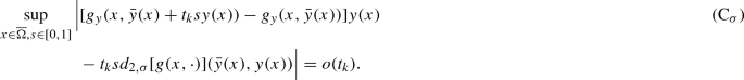
• (H4) The function $g:\overline{\Omega }\times \mathbb {R}\rightarrow \mathbb {R}$ is continuous and Fréchet differentiable wrt the second variable with $g_{y}:\overline{\Omega }\times \mathbb {R}\rightarrow \mathbb {R}$ being also continuous and the following conditions hold:

  • (i) for every $M > 0$, there is $K_{g, M} > 0$ such that for all $x \in \overline{\Omega }$, $y_{1}, y_{2} \in \mathbb {R}$ with $|y_{1}|, |y_{2}| \le M$,

    $$\begin{aligned} |g_{y}(x, y_{1}) - g_{y}(x, y_{2})| \le K_{g, M}|y_{1} - y_{2}|; \end{aligned}$$

  • (ii) there exists the second-order sequential directional derivative $d_{2, \sigma }[g(x, \cdot )](\bar{y}(x), y(x))$ for all $x \in \overline{\Omega }$ and the next condition is verified:

    

• (H5) $h:\Omega \times \mathbb {R}\rightarrow \mathbb {R}$ is a Carathéodory function of class $C^{1}$ wrt the second variable, $h(\cdot , 0) \in L^{p}(\Omega )$ and the following conditions are satisfied:

  • (i)

    • (i.1) $h_{y}(x, \bar{y}) \ge - \phi _{y}(x, y)$ for a.e. $x \in \Omega$ and for all $y \in \mathbb {R}$;

    • (i.2) for every $M > 0$, there is $K_{h, M} > 0$ such that

      $$\begin{aligned} |h_{y}(x, y)| \le K_{h, M}, |h_{y}(x, y_{1}) - h_{y}(x, y_{2})| \le K_{h, M}|y_{1} - y_{2}|, \end{aligned}$$

      for a.e. $x \in \Omega$ and for all $|y|, |y_{1}|, |y_{2}| \le M$;

  • (ii) there exists the second-order sequential directional derivative $d_{2, \sigma }[h(x, \cdot )](\bar{y}(x), y(x))$ for a.e. $x \in \Omega$.

Note that if the function g is of class $C^{2}$ wrt the second variable, then assumption (H4)-(ii) automatically holds and, moreover, condition (C$_{\sigma }$) is valid for all sequence $\sigma = \{t_{k}\}$ with $t_{k} \rightarrow 0^{+}$.

Let us define the sets:

$$\begin{aligned} Q:= \{v \in C(\overline{\Omega }):\, v(x) \ge 0, \forall x \in \overline{\Omega }\}, \end{aligned}$$

(6)

a closed convex cone of nonnegative valued functions in $C(\overline{\Omega })$, and

$$\begin{aligned} D:= \{v \in L^{p}(\Omega ):\, \alpha (x) \le v(x) \le \beta (x) \text{ a.e } x \in \Omega \}, \end{aligned}$$

(7)

a closed convex set in $L^{p}(\Omega )$.

We need the notion of critical direction for the problem under consideration.

Definition 2.1

A pair $d = (y, u) \in W_{0}^{1, r}(\Omega )\times L^{p}(\Omega )$ is said to be a critical direction for problem (OCP) at a feasible point $\bar{z} = (\bar{y}, \bar{u})$ iff the following conditions hold:

• (a) $\int _{\Omega }\big (L_{y}(x, \bar{y}(x), \bar{u}(x))y(x) + L_{u}(x, \bar{y}(x), \bar{u}(x))u(x)\big )dx \le 0$;

• (b) $- \sum _{i, j = 1}^{N}D_{j}(a_{ij}(\cdot )D_{i}y) + \phi _{y}(\cdot , \bar{y})y = u$ in $\Omega$, $y|_{\Gamma } = 0$;

• (c) $g_{y}(x, \bar{y}(x))y(x) \le 0$ for all $x \in \overline{\Omega }$ satisfying $g(x, \bar{y}(x)) = 0$;

• (d) $h_{y}(\cdot , \bar{y})y + u \in$ cl cone$(D - h(\cdot , \bar{y}) - \bar{u})$.

The main result of this paper is stated as below.

Theorem 2.1

Let $\bar{z} = (\bar{y}, \bar{u})$ be a local optimal solution of problem (OCP), $d = (y, u)$ a critical direction, and $\sigma = \{t_{k}\}$ a sequence with $t_{k} \rightarrow 0^{+}$. Suppose that assumptions (H1)–(H5) are fulfilled and the set $T^{i, 2, \sigma }(D, h(\cdot , \bar{y}) + \bar{u}, h_{y}(\cdot , \bar{y})y + u)$ is nonempty. Then, there exist multipliers $\lambda \in \mathbb {R}$, $\varphi \in W_{0}^{1, s}(\Omega )$, $\mu \in \mathcal {M}(\overline{\Omega })$, $\psi \in L^{q}(\Omega )$ with $(\lambda , \mu ) \ne (0, 0)$, $\lambda \ge 0$, $\mu \succeq 0$ for which the following assertions are satisfied:

• (a) (the adjoint equation)

  $$\begin{aligned}&- \sum _{i, j = 1}^{N}D_{i}(a_{ij}(\cdot )D_{j}\varphi ) + \phi _{y}(\cdot , \bar{y})\varphi = - \lambda L_{y}(\cdot , \bar{y}, \bar{u})\\&\quad - [g_{y}(\cdot , \bar{y})]^{*}\mu - [h_{y}(\cdot , \bar{y})]^{*}\psi \,\, \mathrm{in } \,\, \Omega \text{, } \,\, \varphi |_{\Gamma } = 0\text{; } \end{aligned}$$

• (b) (the stationary condition in u)

  $$\begin{aligned} \lambda L_{u}(\cdot , \bar{y}, \bar{u}) - \varphi (x) + \psi (x) = 0 \,\, a.e. \,\, x \in \Omega \text{; } \end{aligned}$$

• (c) (the complementary condition in z)

  $$\begin{aligned} \psi (x) \,\left\{ \begin{array}{lll}\le 0 &{}\quad \text{ a.e. }\,\,\, x \in \Omega _{\alpha }\text{, }\\ \ge 0 &{}\quad \text{ a.e. }\,\,\, x \in \Omega _{\beta }\text{, }\\ = 0 &{}\quad \text{ otherwise, }\,\,\, \\ \end{array} \right. \end{aligned}$$

  where

  $$\begin{aligned} \Omega _{\alpha }:= & {} \{x \in \Omega :\, h(x, \bar{y}(x)) + \bar{u}(x) = \alpha (x)\}\text{, }\\ \Omega _{\beta }:= & {} \{x \in \Omega :\, h(x, \bar{y}(x)) + \bar{u}(x) = \beta (x)\}\text{; } \end{aligned}$$

• (d) (the complementary condition in y)

  $$\begin{aligned} \mathrm{supp}(\mu ) \subset \{x \in \overline{\Omega } \mid g(x, \bar{y}(x)) = 0\}\text{; } \end{aligned}$$

• (e) (the sequence-based second-order condition)

  $$\begin{aligned} \mathcal {L}:= & {} \lambda \int _{\Omega }d_{2, \sigma }[L(x, \cdot , \cdot )](\bar{z}(x), d(x))dx + \int _{\Omega }\varphi (x)d_{2, \sigma }[\phi (x, \cdot )](\bar{y}(x), y(x))dx\nonumber \\&+ \int _{\overline{\Omega }}d_{2, \sigma }[g(x, \cdot )](\bar{y}(x), y(x))d\mu (x) + \int _{\Omega }\psi (x)d_{2, \sigma }[h(x, \cdot )](\bar{y}(x), y(x))dx\nonumber \\&\ge s(\mu , T^{i, 2, \sigma }(-Q, g(\cdot , \bar{y}), g_{y}(\cdot , \bar{y})y)). \end{aligned}$$

  (8)

Let us define the functions on $\overline{\Omega }$ as follows:

$$\begin{aligned} a(x)= & {} - g(x, \bar{y}(x)), b(x) = - g_{y}(x, \bar{y}(x))y(x),\\ \theta ^{g, \sigma }_{\bar{z}, d}(x)= & {} \liminf _{k \rightarrow \infty , x^{'}\rightarrow x}\dfrac{a(x^{'}) + t_{k}b(x^{'})}{\frac{1}{2}t_{k}^{2}}. \end{aligned}$$

Then, by Theorem 4.147 in [5], one has that

$$\begin{aligned} T^{i, 2, \sigma }(-Q, g(\cdot , \bar{y}), g_{y}(\cdot , \bar{y})y) = \{v \in C(\overline{\Omega }):\, v(x) \le \theta ^{g, \sigma }_{\bar{z}, d}(x), \forall x \in \overline{\Omega }\} \end{aligned}$$

and $T^{i, 2, \sigma }(-Q, g(\cdot , \bar{y}), g_{y}(\cdot , \bar{y})y)$ is nonempty iff $\theta ^{g, \sigma }_{\bar{z}, d}(x) > - \infty$, for all $x \in \overline{\Omega }$. In addition, if $T^{i, 2, \sigma }(-Q, g(\cdot , \bar{y}), g_{y}(\cdot , \bar{y})y) \ne \emptyset$, then

$$\begin{aligned} s(\mu , T^{i, 2, \sigma }(-Q, g(\cdot , \bar{y}), g_{y}(\cdot , \bar{y})y)) = \int _{\overline{\Omega }}\theta ^{g, \sigma }_{\bar{z}, d}(x)d\mu (x). \end{aligned}$$

We observe that in the literature, a large number of works handling with necessary second-order optimality conditions, for optimal control problems of partial differential equations, utilize the data that are of class $C^{2}$ wrt the state and/or control variable (see e.g., [5,6,7,8,9, 21,22,23, 29, 36]). However, in the present note, the involved functions of our problem are not assumed to be twice differentiable. We employ directional derivatives and local approximations, dependent on given sequences, in order to analyze new sequence-based second-order Lagrange multiplier rules for nonsmooth optimal control problems, driven by semilinear elliptic equations.

In the next example, we can select some reasonable sequence to reject $\bar{z} = (\bar{y}, \bar{u})$ from suspected couples, which fulfill first-order necessary conditions, for local optimal solutions of problem (OCP). This clarifies the prominent role of sequences in our second-order optimality conditions.

Example 2.1

Let $\Omega$ be the open unit ball in $\mathbb {R}^{2}$ with the boundary $\Gamma$, $p = 2$, and $r > 2$. Let L, g, $a_{ij}$, $\phi$, h, $\alpha$, $\beta$ be respectively given by

$$\begin{aligned} L(x, y, u)= & {} y|y| - u^{2}, \,\, g(x, y) = - x_{1}^{2} - x_{2}^{2} + y|y|,\\ a_{ij}(x)= & {} \,\left\{ \begin{array}{ll} 1 &{}\quad \text{ if }\,\,\, i = j,\\ 0 &{}\quad \text{ if }\,\,\, i \ne j,\\ \end{array} \right. \phi (x, y) = y^{3} + y,\\ h(x, y)= & {} \,\left\{ \begin{array}{ll} \frac{1}{3}y^{3} + y^{2}\sin (\ln |y|) + y &{} \quad \text{ if } \,\,\, y \ne 0,\\ 0 &{}\quad \text{ if } \,\,\, y = 0,\\ \end{array} \right. \\ \alpha (x)= & {} - 1, \,\, \beta (x) = 1, \end{aligned}$$

where $x = (x_{1}, x_{2})$. Then, L, g and h are in $C^{1, 1}$ but not in $C^{2}$, $\phi$ is a $C^{2}$ function, and we have

$$\begin{aligned} L_{y}(x, y, u)= & {} 2|y|, \,\, L_{u}(x, y, u) = - 2u,\\ g_{y}(x, y)= & {} 2|y|, \,\, \phi _{y}(x, y) = 3y^{2} + 1,\\ h_{y}(x, y)= & {} \,\left\{ \begin{array}{ll} y^{2} + [2\sin (\ln |y|) + \cos (\ln |y|)]y + 1 &{}\quad \text{ if } \,\,\, y \ne 0,\\ 1 &{}\quad \text{ if } \,\,\, y = 0.\\ \end{array} \right. \end{aligned}$$

Let us show that the feasible couple $\bar{z} = (\bar{y}, \bar{u}) \equiv (0, 0)$ is not a local optimal solution of problem (OCP). Let $(\lambda , \varphi , \mu , \psi )$ be a tuple of Lagrange multipliers such that $(\lambda , \mu ) \ne (0, 0)$, $\lambda \ge 0$, $\mu \succeq 0$, and assertions (a)-(d) in Theorem 2.1 are fulfilled at $\bar{z}$. Then, $\varphi \equiv 0$, $\psi \equiv 0$, and for some $\tau \ge 0$, one gets

$$\begin{aligned} \langle \mu , v\rangle = \tau v(0), \,\, \forall v \in C(\overline{\Omega }). \end{aligned}$$

Let us choose $d = (y, u)$ as a critical direction for the problem at $\bar{z}$, where

$$\begin{aligned} y(x) = x_{1}^{2} + x_{2}^{2} - 1, \,\, u(x) = x_{1}^{2} + x_{2}^{2} - 5 \end{aligned}$$

and pick the sequence $\sigma = \{t_{k}\}$ with $t_{k} = \exp (- k2\pi )$. Then, it is not difficult to check that $0 \in T^{i, 2, \sigma }(D, h(\cdot , \bar{y}) + \bar{u}, h_{y}(\cdot , \bar{y})y + u)$ and all assumptions (H1)-(H5) hold true. Moreover, we obtain

$$\begin{aligned}&d_{2, \sigma }[L(x, \cdot , \cdot )](\bar{z}(x), d(x)) = 2y(x)|y(x)| - 2[u(x)]^{2},\\&d_{2, \sigma }[g(x, \cdot )](\bar{y}(x), y(x)) = 2y(x)|y(x)|, \,\, d_{2, \sigma }[\phi (x, \cdot )](\bar{y}(x), y(x)) = 0,\\&d_{2, \sigma }[h(x, \cdot )](\bar{y}(x), y(x)) = \,\left\{ \begin{array}{ll} 2[y(x)]^{2}\sin (\ln |y(x)|) &{}\quad \text{ if }\,\,\, x \not \in \Gamma ,\\ 0 &{}\quad \text{ if }\,\,\, x \in \Gamma ,\\ \end{array} \right. \\&\theta ^{g, \sigma }_{\bar{z}, d}(x) = \,\left\{ \begin{array}{ll} + \infty &{}\quad \text{ if }\,\,\, x \ne 0,\\ 0 &{}\quad \text{ if }\,\,\, x = 0.\\ \end{array} \right. \end{aligned}$$

Thus, for every tuple of Lagrange multipliers as above, one has

$$\begin{aligned} \mathcal {L}= & {} \lambda \int _{\Omega }\big (2y(x)|y(x)| - 2[u(x)]^{2}\big )dx + \int _{\overline{\Omega }}2y(x)|y(x)|d\mu (x)\\= & {} - 124\pi \lambda /3 - 2\tau < 0 = \int _{\overline{\Omega }}\theta ^{g, \sigma }_{\bar{z}, d}(x)d\mu (x), \end{aligned}$$

where the amount $\mathcal {L}$ is defined in assertion (e) of Theorem 2.1. According to this theorem, we claim that $\bar{z}$ is not a local optimal solution of our problem.

3 Sequence-based necessary second-order optimality conditions for a nonsmooth optimization problem

3.1 Notations, preliminaries and preliminary results

In this subsection, we present preliminaries and preliminary results, related to some notions of tangent cone, second-order sequential local approximation, second-order sequential directional derivative and directional metric subregularity, that will be needed in the paper.

Throughout the paper, $\mathbb {N}$, $\mathbb {R}$ and $\mathbb {R}_{+}$ stand for the set of natural numbers, the one of real numbers and the set of nonnegative real numbers, respectively. For a normed space E, $E^{*}$ denotes the topological dual of E, $\langle \cdot ,\cdot \rangle$ the canonical pairing and $\Vert \cdot \Vert _{E}$ the norm in E. For given a set $M \subseteq E$ and an element $x^* \in E^*$, we define $s(x^*, M):= \sup _{m \in M}\langle x^*, m\rangle$. d(y, S) is used for the distance from a point y to a set S. $B_{E}(x, r):= \{y \in E : \Vert x - y\Vert _{E} < r\}$ and for $B_{E}(0, 1)$ we write simply $B_{E}$. For a cone $C \subset E$, the positive polar cone of C is $C^{*}:= \{c^{*} \in E^{*}:\, \langle c^{*}, c\rangle \ge 0, \,\, \forall c \in C\}$. For a set $A \subset E$, let core A be its algebraic interior, int A its topological interior, cl A (or $\overline{A}$) its closure, and cone A its conical hull. For $n \in \mathbb {N}$, $o(t^{n})$ designates a point in a considered space (which is clear from the context) depending on t such that $o(t^{n})/t^{n} \rightarrow 0$ as $t \rightarrow 0^{+}$.

For a bounded domain $\Omega \subset \mathbb {R}^{N}$ with $N \in \mathbb {N}$, $C(\overline{\Omega })$ stands for the Banach space of all continuous real functions defined on the compact metric space $\overline{\Omega }$ and is furnished with the sup-norm. The dual space of $C(\overline{\Omega })$, written as $\mathcal {M}(\overline{\Omega })$, is the linear space of real and regular Borel measures on $\overline{\Omega }$. For $\mu \in \mathcal {M}(\overline{\Omega })$, the support of $\mu$, denoted by $\text{ supp }(\mu )$, is the smallest closed subset of $\overline{\Omega }$ such that $\mu (\Omega {\setminus } \text{ supp }(\mu )) = 0$. By $\mu \succeq 0$ we mean that $\mu (A) \ge 0$ for any $A \in \mathcal {B}$, where $\mathcal {B}$ is the Borel sigma-algebra of $\overline{\Omega }$. Partial derivatives are denoted by subscripts: $f_{y}: = \frac{\partial f}{\partial y}$ and $f_{u}: = \frac{\partial f}{\partial u}$ for a mapping f.

Let us recall some concepts of tangent cone that we will subsequently utilize. Let E be a normed space, S a subset of E, $x_{0} \in \overline{S}$ and $u \in E$. The contingent (resp, inner) tangent cone of S at $x_{0}$ is

$$\begin{aligned}&T(S, x_{0}):= \{v \in E:\, \exists t_{k} \rightarrow 0^{+}, \exists v_{k} \rightarrow v, \forall k \in \mathbb {N}, x_{0} + t_{k}v_{k} \in S\}\\&\Big (\mathrm{resp,} \,\, T^{i}(S, x_{0}):= \{v \in E:\, \forall t_{k} \rightarrow 0^{+}, \exists v_{k} \rightarrow v, \forall k \in \mathbb {N}, x_{0} + t_{k}v_{k} \in S\}\Big ). \end{aligned}$$

The interior tangent cone (resp, Clarke interior tangent cone) of S at $x_{0}$ is

It is known that, if the set S is convex, then $T(S, x_{0}) = T^{i}(S, x_{0})$.

As in [5], we define the normal cone to S at $x_{0}$ by

$$\begin{aligned} N(S, x_{0}):= -[T(S, x_{0})]^*. \end{aligned}$$

The following notions of second-order sequential local approximation were proposed in [5, 37].

Definition 3.1

Let $\sigma \in \Sigma$ be a sequence, where $\Sigma := \{\sigma = \{t_{k}\}\mid t_{k} \rightarrow 0^{+}\}$.

• (a) The second-order contingent tangent set of S at $(x_{0}, u)$ wrt $\sigma$ is

  $$\begin{aligned} T^{i, 2, \sigma }(S, x_{0}, u):= \left\{ w \in E:\, \exists w_{k} \rightarrow w, \forall k \in \mathbb {N}, x_{0} + t_{k}u + \frac{1}{2}t_{k}^{2}w_{k} \in S\right\} . \end{aligned}$$

• (b) The second-order interior tangent set of S at $(x_{0}, u)$ wrt $\sigma$ is

  $$\begin{aligned} IT^{2, \sigma }(S, x_{0}, u):= \left\{ w \in E:\, \forall w_{k} \rightarrow w, \forall k \,\, \mathrm{large \,\, enough}, x_{0} + t_{k}u + \frac{1}{2}t_{k}^{2}w_{k} \in S\right\} . \end{aligned}$$

We mention that every contingent tangent set is closed, but the interior one is open. When S is convex, so is $T^{i, 2, \sigma }(S, x_{0}, u)$ (and $IT^{2, \sigma }(S, x_{0}, u)$) for any $\sigma \in \Sigma$.

The next facts, whose proof can be found in [37], give some basic properties of second-order local approximations.

Proposition 3.1

Let $S \subset E$, $x_{0} \in \overline{S}$, $u \in E$, and $\sigma \in \Sigma$. Then, the following are satisfied.

• (a) $IT^{2, \sigma }(S, x_{0}, u) \subset T^{i, 2, \sigma }(S, x_{0}, u) \subset \text{ cl } \text{ cone[cone }(S - x_{0}) - u]$.

• (b) If $IT_{C}(S, x_{0}) \ne \emptyset$ and $T^{i, 2, \sigma }(S, x_{0}, u) \ne \emptyset$, then

  $$\begin{aligned} \mathrm{cl} \,\, IT^{2, \sigma }(S, x_{0}, u) = T^{i, 2, \sigma }(S, x_{0}, u). \end{aligned}$$

  Let, in addition, S be convex and $x_{0} \in S$. One has the following.

• (c) $T^{i, 2, \sigma }(S, x_{0}, u) + T(T(S, x_{0}), u) \subset T^{i, 2, \sigma }(S, x_{0}, u) \subset T(T(S, x_{0}), u)$.

• (d) If $T^{i, 2, \sigma }(S, x_{0}, u) \ne \emptyset$ and $e^{*} \in E^{*}$ such that $s(e^*, T^{i, 2, \sigma }(S, x_{0}, u)) < +\infty$, then $e^{*} \in N(S, x_{0})$ and $\langle e^{*}, u\rangle = 0$, i.e. $e^{*} \in - [T(T(S, x_{0}), u)]^{*}$.

Let E and F be normed spaces, $\phi :E \rightarrow F$ a mapping and $x_{0}, u \in E$. We say that $\phi$ is strictly differentiable at $x_{0}$ iff it has Fréchet derivative $\triangledown \phi (x_{0})$ at $x_{0}$ and

$$\begin{aligned} \lim _{x \rightarrow x_{0}, x^{'} \rightarrow x_{0}}\dfrac{\Vert \phi (x) - \phi (x^{'}) - \triangledown \phi (x_{0})(x - x^{'})\Vert _{F}}{\Vert x - x^{'}\Vert _{E}} = 0. \end{aligned}$$

Obviously, if $\phi$ is strictly differentiable at $x_{0}$, then $\phi$ is locally Lipschitz at $x_{0}$.

In this paper, we concern with the following second-order sequential directional derivative, which was introduced by Gfrerer [15] (see also [38]).

Definition 3.2

Let $\sigma = \{t_{k}\} \in \Sigma$ and $\phi$ be Fréchet differentiable at $x_{0}$. The second-order sequential directional derivative of $\phi$ at $x_{0}$ in direction u wrt $\sigma$ is

$$\begin{aligned} d_{2, \sigma }\phi (x_{0}, u):= \lim _{k \rightarrow \infty }\dfrac{\phi (x_{0} + t_{k}u) - \phi (x_{0}) - t_{k}\triangledown \phi (x_{0})u}{t_{k}^{2}/2}, \end{aligned}$$

when the limit on the right-hand side exists as an element in the space F.

The next result is a direct consequence of the definition.

Proposition 3.2

Let $x_{0}, u \in E$ and $\phi :E \rightarrow F$. Then, the following assertions are fulfilled.

• (a) If $\phi$ is strictly differentiable at $x_{0}$, then for all $\sigma = \{t_{k}\} \in \Sigma$ such that $d_{2, \sigma }\phi (x_{0}, u)$ exists and for all $w_{k} \rightarrow w$ in E, one has

  $$\begin{aligned} \lim _{k \rightarrow \infty }\dfrac{\phi (x_{0} + t_{k}u + \frac{1}{2}t_{k}^{2}w_{k}) - \phi (x_{0}) - t_{k}\triangledown \phi (x_{0})u}{t_{k}^{2}/2} = \triangledown \phi (x_{0})w + d_{2, \sigma }\phi (x_{0}, u). \end{aligned}$$

• (b) If $\phi$ is twice Fréchet differentiable at $x_{0}$, then

  $$\begin{aligned} d_{2, \sigma }\phi (x_{0}, u) = \triangledown ^{2}\phi (x_{0})(u, u), \,\, \forall \sigma \in \Sigma , \end{aligned}$$

  where $\triangledown ^{2}\phi (x_{0})$ is the twice Fréchet derivative of $\phi$ at $x_{0}$.

Some computations for the second-order sequential directional derivative are illustrated as below.

Example 3.1

• (a) Let $x_{0} = 0$, $u \in \mathbb {R}$ and $\phi :\mathbb {R} \rightarrow \mathbb {R}$ be given by $\phi (x) = x|x|$. Then, $\phi$ is in $C^{1, 1}$ but not twice Fréchet differentiable at $x_{0}$. Moreover, we have for every $\sigma \in \Sigma$,

  $$\begin{aligned} d_{2, \sigma }\phi (x_{0}, u) = 2u|u|. \end{aligned}$$

• (b) Let $\phi :\mathbb {R} \rightarrow \mathbb {R}$ be defined as $\phi (x) = x^{2}\sin (\ln |x|)$ if $x \ne 0$ and $\phi (0) = 0$. Let $x_{0} = 0$ and $u \in \mathbb {R} \setminus \{0\}$. Then, $\phi$ is in $C^{1, 1}$ but not twice Fréchet differentiable at $x_{0}$. Further, for any given $\alpha \in \mathbb {R}$, one obtains for $\sigma _{\alpha } = \{t_{k}\} \in \Sigma$ with $t_{k} = \exp (- k2\pi + \alpha )$,

  $$\begin{aligned} d_{2, \sigma _{\alpha }}\phi (x_{0}, u) = 2u^{2}\sin (\ln |u| + \alpha ). \end{aligned}$$

  However, for any given $\beta \in \mathbb {R} \setminus \{0\}$, we see that $d_{2, \sigma _{\beta }}\phi (x_{0}, u)$ does not exist for $\sigma _{\beta } = \{t_{k}\} \in \Sigma$ with $t_{k} = \beta ^{2}\exp (- k)$.

• (c) Let $x_{0} = 0$, $u \in \mathbb {R} \setminus \{0\}$ and $\phi :\mathbb {R} \rightarrow \mathbb {R}$ be given by $\phi (x) = x^{2}\ln |x|$ if $x \ne 0$, and $\phi (0) = 0$. Then, $\phi$ is strictly differentiable but not in $C^{1, 1}$ at $x_{0}$, and one observes that $d_{2, \sigma }\phi (x_{0}, u)$ is not in existence for all $\sigma \in \Sigma$.

Now, let us recall the concept of directional metric subregularity which will be used to derive necessary optimality conditions for problem (P) below.

Definition 3.3

([16, 35]) Let $x_{0}, u \in E$, $S \subset E$, $D \subset F$ and $\phi :E \rightarrow F$. One says that the mapping $\phi$ is directionally metrically subregular at $(x_{0}, u)$ wrt (S, D) iff there exist $\mu > 0$, $\rho > 0$ such that, for every $t\in (0, \rho )$ and $v \in B_{E}(u, \rho )$ with $x_{0} + tv \in S$,

Notice that if the sets S and D are closed and convex, the mapping $\phi$ is strictly differentiable at $x_{0}$, and the following Robinson constraint qualification holds:

$$\begin{aligned} \triangledown \phi (x_{0})(\text{ cone }(S - x_{0})) - \text{ cone }(D - \phi (x_{0})) = F, \end{aligned}$$

then condition (DMSR$_u$) of $\phi$ wrt (S, D) is fulfilled for all $u \in E$.

The next fact shows a sequence-based characterization of the second-order contingent tangent set of $S\cap \phi ^{-1}(D)$ at $(x_{0}, u)$ wrt $\sigma$.

Proposition 3.3

Let $x_{0} \in S\cap \phi ^{-1}(D)$, $u \in E$, and $\sigma \in \Sigma$ be given. Assume that the mapping $\phi$ is strictly differentiable at $x_{0}$ for which the directional derivative $d_{2, \sigma }\phi (x_{0}, u)$ exists and condition $(\mathrm{DMSR}_{u})$ of $\phi$ wrt (S, D) is satisfied. Then, we have

Proof

Let $\sigma = \{t_{k}\}$. Let $w \in T^{i, 2, \sigma }(S\cap \phi ^{-1}(D), x_{0}, u)$. Then, there is $w_{k} \rightarrow w$ such that $x_{k}:= x_{0} + t_{k}u + \frac{1}{2}t_{k}^{2}w_{k} \in S\cap \phi ^{-1}(D)$. Thus, $w \in T^{i, 2, \sigma }(S, x_{0}, u)$ and $\phi (x_{k}) \in D$. By virtue of Proposition 3.2 (a), one gets

$$\begin{aligned} \dfrac{\phi (x_{k}) - \phi (x_{0}) - t_{k}\triangledown \phi (x_{0})u}{t_{k}^{2}/2} \rightarrow \triangledown \phi (x_{0})w + d_{2, \sigma }\phi (x_{0}, u), \end{aligned}$$

which results that $\triangledown \phi (x_{0})w + d_{2, \sigma }\phi (x_{0}, u) \in T^{i, 2, \sigma }(D, \phi (x_{0}), \triangledown \phi (x_{0})u)$.

For the reversion, suppose that $w \in T^{i, 2, \sigma }(S, x_{0}, u)$ and $y:= \triangledown \phi (x_{0})w + d_{2, \sigma }\phi (x_{0}, u) \in T^{i, 2, \sigma }(D, \phi (x_{0}), \triangledown \phi (x_{0})u)$. Then, there exist $w_{k} \rightarrow w$ and $y_{k} \rightarrow y$ such that $x_{0} + t_{k}u + \frac{1}{2}t_{k}^{2}w_{k} \in S$ and $\phi (x_{0}) + t_{k}\triangledown \phi (x_0)u + \frac{1}{2}t_{k}^{2}y_{k} \in D$ for all k. It follows from Proposition 3.2 (a) that

$$\begin{aligned} \dfrac{\phi (x_{0} + t_{k}u + \frac{1}{2}t_{k}^{2}w_{k}) - \phi (x_{0}) - t_{k}\triangledown \phi (x_{0})u}{t_{k}^{2}/2} \rightarrow y. \end{aligned}$$

According to the directional metric subregularity of $\phi$, we obtain $\mu > 0$ such that, for every large k, $d(x_{0} + t_{k}u + \frac{1}{2}t_{k}^{2}w_{k}, S\cap \phi ^{-1}(D)) \le \mu d(\phi (x_{0} + t_{k}u + \frac{1}{2}t_{k}^{2}w_{k}), D)$. Therefore, for large k, there exists $\bar{w}_{k}: x_{0} + t_{k}u + \frac{1}{2}t_{k}^{2}\bar{w}_{k} \in S\cap \phi ^{-1}(D)$ such that $\frac{1}{2}t_{k}^{2}\Vert w_{k} - \bar{w}_{k}\Vert \le \mu \Vert \phi (x_{0} + t_{k}u + \frac{1}{2}t_{k}^{2}w_{k}) - \phi (x_{0}) - t_{k}\triangledown \phi (x_{0})u - \frac{1}{2}t_{k}^{2}y_{k}\Vert + o(t_{k}^{2})$, and so, $\bar{w}_{k} \rightarrow w$. In consequence, $w \in T^{i, 2, \sigma }(S\cap \phi ^{-1}(D), x_{0}, u)$. $\square$

3.2 Sequence-based necessary second-order optimality conditions

In this subsection, using sequential directional derivatives and sequential tangent sets, we develop sequence-based necessary second-order optimality conditions for the following nonsmooth optimization problem with mixed constraints:

$$\begin{aligned} \text{ min } \,\, J(z), \mathrm{\,\, subject \,\, to \,\,} \Phi (z) = 0, \,\, G(z) \in - Q, \,\, H(z) \in D. \end{aligned}$$

(P)

Here, $J:Z \rightarrow \mathbb {R}$, $\Phi :Z \rightarrow \Pi$, $G:Z \rightarrow \Lambda$ and $H:Z \rightarrow \Delta$ are mappings, Z, $\Pi$ and $\Delta$ Banach spaces, $\Lambda$ a normed space, $Q \subset \Lambda$ a convex set with nonempty interior, and $D \subset \Delta$ a nonempty convex set with possibly empty interior.

The feasible set of problem (P) is

$$\begin{aligned} \mathcal {F}_{P}:= \{z \in Z:\, z \in S, \,\, G(z) \in -Q, \,\, H(z) \in D \}, \end{aligned}$$

where $S:= \{z \in Z:\, \Phi (z) = 0\}$.

A point $\bar{z} \in \mathcal {F}_{P}$ is called a local optimal solution of (P) iff there exists a neighborhood $\mathcal {U}$ of $\bar{z}$ such that, for all $z \in \mathcal {U}\cap \mathcal {F}_{P}$,

$$\begin{aligned} J(z) - J(\bar{z}) \ge 0. \end{aligned}$$

Set $Q(G(\bar{z})):=$ cone$(Q + G(\bar{z}))$. Then, $T(-Q, G(\bar{z})) = - \text{ cl } Q(G(\bar{z}))$ and $N(-Q, G(\bar{z})) = [Q(G(\bar{z}))]^{*}$. Note that, if Q is a convex cone, then

$$\begin{aligned} {[}Q(G(\bar{z}))]^{*}=\{\lambda ^{*} \in Q^{*}:\,\langle \lambda ^{*}, G(\bar{z})\rangle = 0\}. \end{aligned}$$

The proof of the next first-order (resp, second-order) primal necessary condition for problem (P) can be proceeded similarly as the one of Theorem 3.2 (resp, Theorem 3.6) in [38], with some minor modifications.

Proposition 3.4

Let $\bar{z}$ be a local optimal solution of (P). Then, one has the following.

• (a) Let $d \in T^{i}(S, \bar{z}) \setminus \{0\}$ be a given direction. Assume that the mapping (J, G, H) is Fréchet differentiable at $\bar{z}$ and condition $(\mathrm{DMSR}_{d})$ of H wrt (S, D) satisfied. Then,

  $$\begin{aligned} \triangledown (J, G, H)(\bar{z})d \bigcap -\mathrm{int}[\mathbb {R}_{+}\times Q(G(\bar{z}))]\times T(D, H(\bar{z})) = \emptyset . \end{aligned}$$

• (b) Let $d \in Z$ be a direction such that

  $$\begin{aligned} d \in T^{i}(S, \bar{z}) \,\, \text{ and } \,\, \triangledown (J, G, H)(\bar{z})d \in - [\mathbb {R}_{+}\times \mathrm{cl}\,\, Q(G(\bar{z}))]\times T(D, H(\bar{z})). \end{aligned}$$

  Suppose that the mapping (J, G, H) is strictly differentiable at $\bar{z}$ and condition $(\mathrm{DMSR}_{d})$ of H wrt (S, D) fulfilled. Then, for every sequence $\sigma \in \Sigma$ such that the directional derivative $d_{2, \sigma }(J, G, H)(\bar{z}, d)$ exists and for every $z \in T^{i, 2, \sigma }(S, \bar{z}, d)$, we have

  $$\begin{aligned}&\triangledown (J, G, H)(\bar{z})z + d_{2, \sigma }(J, G, H)(\bar{z}, d)\\&\quad \not \in (-\infty , 0)\times IT^{2, \sigma }(-Q, G(\bar{z}), \triangledown G(\bar{z})d)\times T^{i, 2, \sigma }(D, H(\bar{z}), \triangledown H(\bar{z})d). \end{aligned}$$

The following fact will be used to obtain necessary optimality conditions via Lagrange multipliers.

Lemma 3.1

(Lemma 3.3 of [38]) Let E and N be Banach spaces, M a normed space, A a nonempty closed convex subset of E, B a convex subset of M with int $B \ne \emptyset$, R a nonempty closed convex subset of N, and $(\overline{m}, \overline{n}) \in M\times N$ a fixed pair. Let $\zeta :E \rightarrow M$ and $\eta :E \rightarrow N$ be continuous linear mappings. Assume that, for all $e \in A$,

$$\begin{aligned} (\zeta , \eta )(e) + (\overline{m}, \overline{n}) \not \in (-\mathrm{int} \,\, B)\times R. \end{aligned}$$

If $0 \in \mathrm{core}[\eta (A) - R + \overline{n}]$, then there is a triple $(e^*, m^*, n^*) \in E^*\times M^*\times N^*$ with $m^* \ne 0$ such that

$$\begin{aligned}&m^*\circ \zeta + n^*\circ \eta - e^* = 0,\\&\quad \langle m^*, \overline{m}\rangle + \langle n^*, \overline{n}\rangle + \inf _{a \in A}\langle e^*, a\rangle + \inf _{b \in B}\langle m^*, b\rangle \ge \sup _{r \in R}\langle n^*, r\rangle . \end{aligned}$$

Definition 3.4

Suppose that the mapping $(J, \Phi , G, H)$ is Fréchet differentiable at a point $\bar{z} \in \mathcal {F}_{P}$. One says that an element $d \in Z$ is a critical direction for (P) at $\bar{z}$ iff

$$\begin{aligned} \triangledown \Phi (\bar{z})d = 0, \,\, \triangledown J(\bar{z})d \le 0, \, \, \triangledown G(\bar{z})d \in -\mathrm{cl\,\,} Q(G(\bar{z})) \,\, \mathrm{and} \,\, \triangledown H(\bar{z})d \in T(D, H(\bar{z})). \end{aligned}$$

The next theorem shows our main result in this section. With the help of Proposition 3.4 (a) (resp, (b)) and Lemma 3.1, we can prove first-order (resp, second-order sequence-based) dual necessary conditions for problem (P) as below.

Theorem 3.1

Let $\bar{z}$ be a local optimal solution of (P). Then, the following hold.

• (a) Let the mapping (J, G, H) be Fréchet differentiable at $\bar{z}$, and the map $\Phi$ strictly differentiable at $\bar{z}$ with $\triangledown \Phi (\bar{z})$ surjective. Assume that condition $(\mathrm{DMSR}_{d})$ of H wrt (S, D) is fulfilled for all direction $d \ne 0$ for which $\triangledown \Phi (\bar{z})d = 0$, and the following constraint qualification satisfied

  $$\begin{aligned} \triangledown H(\bar{z})T(S, \bar{z}) - T(D, H(\bar{z})) = \Delta . \end{aligned}$$

  (CQ)

  Then, there exists a tuple $(v^{*}, \pi ^{*}, \lambda ^{*}, \delta ^*) \in \mathbb {R}_{+}\times \Pi ^*\times N(-Q, G(\bar{z}))\times N(D, H(\bar{z}))$ with $(v^{*}, \lambda ^{*}) \ne (0, 0)$ such that

  $$\begin{aligned} v^{*}\triangledown J(\bar{z}) + \pi ^{*}\circ \triangledown \Phi (\bar{z}) + \lambda ^{*}\circ \triangledown G(\bar{z}) + \delta ^*\circ \triangledown H(\bar{z}) = 0. \end{aligned}$$

  (9)

• (b) Let $d \in Z$ be a critical direction, and the mapping $(J, \Phi , G, H)$ strictly differentiable at $\bar{z}$ with $\triangledown \Phi (\bar{z})$ surjective. Suppose that condition $(\mathrm{DMSR}_{d})$ of H wrt (S, D) is verified, and the following constraint qualification (dependent on d) holds

  

  Then, for every sequence $\sigma \in \Sigma$ such that the sets $T^{i, 2, \sigma }(-Q, G(\bar{z}), \triangledown G(\bar{z})d)$ and $T^{i, 2, \sigma }(D, H(\bar{z}), \triangledown H(\bar{z})d)$ are nonempty and the directional derivative $d_{2, \sigma }(J, \Phi , G, H)(\bar{z}, d)$ exists, there is a tuple $(v^{*}, \pi ^{*}, \lambda ^{*}, \delta ^*) \in \mathbb {R}_{+}\times \Pi ^*\times N(-Q, G(\bar{z}))\times N(D, H(\bar{z}))$ with $(v^{*}, \lambda ^{*}) \ne (0, 0)$ for which one has (9) and

  $$\begin{aligned}&v^{*}d_{2, \sigma }J(\bar{z}, d) + \langle \pi ^{*}, d_{2, \sigma }\Phi (\bar{z}, d)\rangle + \langle \lambda ^{*}, d_{2, \sigma }G(\bar{z}, d)\rangle + \langle \delta ^*, d_{2, \sigma }H(\bar{z}, d) \rangle \nonumber \\&\quad \ge s(\lambda ^*, T^{i, 2, \sigma }(-Q, G(\bar{z}), \triangledown G(\bar{z})d)) + s(\delta ^*, T^{i, 2, \sigma }(D, H(\bar{z}), \triangledown H(\bar{z})d)).\nonumber \\ \end{aligned}$$

  (10)

Proof

(a) It follows from Proposition 3.3 that

$$\begin{aligned} T(S, \bar{z}) = T^{i}(S, \bar{z}) = \{z \in Z :\, \triangledown \Phi (\bar{z})z = 0\}. \end{aligned}$$

From the surjectivity of $\triangledown \Phi (\bar{z})$ and condition (CQ), we deduce that

$$\begin{aligned} \triangledown (H, \Phi )(\bar{z})Z - T(D, H(\bar{z}))\times \{0\} = \Delta \times \Pi . \end{aligned}$$

By Proposition 3.4 (a), one has for all $d \in Z$,

$$\begin{aligned} (\triangledown (J, G)(\bar{z}), \triangledown (H, \Phi )(\bar{z}))d \not \in -\mathrm{int}[\mathbb {R}_{+}\times Q(G(\bar{z}))]\times T(D, H(\bar{z}))\times \{0\}. \end{aligned}$$

Making use of Lemma 3.1 with $E = Z, M = \mathbb {R}\times \Lambda , N = \Delta \times \Pi$, $A = Z$, $B = \mathbb {R}_{+}\times Q(G(\bar{z}))$, $R = T(D, H(\bar{z}))\times \{0\}$, $\overline{m} = (0, 0)$, $\overline{n} = (0, 0)$, $\zeta = \triangledown (J, G)(\bar{z})$, and $\eta = \triangledown (H, \Phi )(\bar{z})$ gives $(v^{*}, \lambda ^{*}, \delta ^{*}, \pi ^*) \in \mathbb {R}\times \Lambda ^{*}\times \Delta ^{*}\times \Pi ^*$ with $(v^{*}, \lambda ^{*}) \ne (0, 0)$ such that one obtains (9) and

$$\begin{aligned} \inf _{(v, \lambda ) \in \mathbb {R}_{+}\times Q(G(\bar{z}))} \{v^{*}v + \langle \lambda ^{*}, \lambda \rangle \}\ge \sup _{\delta \in T(D, H(\bar{z}))}\langle \delta ^{*}, \delta \rangle . \end{aligned}$$

Since $\mathbb {R}_{+}$, $Q(G(\bar{z}))$ and $T(D, H(\bar{z}))$ are cones, the above inequality yields that $v^{*} \in \mathbb {R}_{+}, \lambda ^{*} \in N(-Q, G(\bar{z}))$ and $\delta ^{*} \in N(D, H(\bar{z}))$.

(b) Due to Proposition 3.3, we get

$$\begin{aligned} T^{i, 2, \sigma }(S, \bar{z}, d) = \{z \in Z :\, \triangledown \Phi (\bar{z})z + d_{2, \sigma }\Phi (\bar{z}, d) = 0\}. \end{aligned}$$

Taking into account Proposition 3.4 (b), one has for all $z \in Z$,

$$\begin{aligned}&(\triangledown (J, G)(\bar{z}), \triangledown (H, \Phi )(\bar{z}))z + (d_{2, \sigma }(J, G)(\bar{z}, d), d_{2, \sigma }(H, \Phi )(\bar{z}, d))\\&\quad \not \in (-\infty , 0)\times IT^{2, \sigma }(-Q, G(\bar{z}), \triangledown G(\bar{z})d)\times T^{i, 2, \sigma }(D, H(\bar{z}), \triangledown H(\bar{z})d)\times \{0\}. \end{aligned}$$

By condition $\mathrm{(CQ}_{{d}}$) and the property of $T^{i, 2, \sigma }$ (see Proposition 3.1 (c)), we obtain

$$\begin{aligned} \triangledown H(\bar{z})T(S, \bar{z}) - T^{i, 2, \sigma }(D, H(\bar{z}), \triangledown H(\bar{z})d) = \Delta . \end{aligned}$$

This together with the surjectivity of $\triangledown \Phi (\bar{z})$ imply that

$$\begin{aligned} \triangledown (H, \Phi )(\bar{z})Z - T^{i, 2, \sigma }(D, H(\bar{z}), \triangledown H(\bar{z})d)\times \{0\} = \Delta \times \Pi . \end{aligned}$$

Applying Lemma 3.1 with $A = Z$, $-B = (-\infty , 0)\times IT^{2, \sigma }(-Q, G(\bar{z}), \triangledown G(\bar{z})d)$, $R = T^{i, 2, \sigma }(D, H(\bar{z}), \triangledown H(\bar{z})d) \times \{0\}$, $\overline{m} = d_{2, \sigma }(J, G)(\bar{z}, d)$, $\overline{n} = d_{2, \sigma }(H, \Phi )(\bar{z}, d)$, $\zeta = \triangledown (J, G)(\bar{z})$, $\eta = \triangledown (H, \Phi )(\bar{z})$, and using Proposition 3.1 (b), we receive $(v^*, \lambda ^*, \delta ^*, \pi ^*) \in \mathbb {R}\times \Lambda ^{*}\times \Delta ^{*}\times \Pi ^*$ with $(v^{*}, \lambda ^{*}) \ne (0, 0)$ such that one gets (9) and for all $v > 0$, $\lambda \in T^{i, 2, \sigma }(-Q, G(\bar{z}), \triangledown G(\bar{z})d)$ and $\delta \in T^{i, 2, \sigma }(D, H(\bar{z}), \triangledown H(\bar{z})d)$,

$$\begin{aligned}&v^{*}d_{2, \sigma }J(\bar{z}, d) + \langle \lambda ^{*}, d_{2, \sigma }G(\bar{z}, d)\rangle + \langle \delta ^{*}, d_{2, \sigma }H(\bar{z}, d)\rangle + \langle \pi ^*, d_{2, \sigma }\Phi (\bar{z}, d)\rangle + v^{*}v \\&\quad \ge \langle \lambda ^{*}, \lambda \rangle + \langle \delta ^{*}, \delta \rangle . \end{aligned}$$

It entails that $v^{*} \in \mathbb {R}_{+}$. By this and Proposition 3.1 (d), we derive from the latter inequality that $\lambda ^{*} \in N(-Q, G(\bar{z}))$ with $\langle \lambda ^{*}, \triangledown G(\bar{z})d\rangle = 0$, $\delta ^{*} \in N(D, H(\bar{z}))$ fulfilling $\langle \delta ^{*}, \triangledown H(\bar{z})d\rangle = 0$, and the second-order necessary condition (10) is satisfied. $\square$

It is worth mentioning that some sequence-based necessary second-order optimality conditions were established in several recent articles, see [19] for unconstrained composite minimization problems involving twice differentiable core functions, [5] for smooth scalar optimization problems with constraints, [2, 31] for constrained optimum problems under differentiability wrt approximation hypothesis of the data, [15] for second-order sequentially directionally differentiable vector optimization problems with a smoothness assumption imposed on the data, and [37, 38] for nonsmooth vector optimization problems with mixed constraints but without the constraint $\Phi (z) = 0$.

4 Proof of Theorem 2.1

In this section, we prove the main result of the paper. To do this, we reduce problem (OCP) to problem (P) and then apply Theorem 3.1. Let us set the spaces

$$\begin{aligned} Y= & {} W_{0}^{1, r}(\Omega ), \,\, U = L^{p}(\Omega ), \,\, Z = Y\times U,\\ \Pi= & {} W^{-1, r}(\Omega ), \,\, \Lambda = C(\overline{\Omega }), \,\, \Delta = L^{p}(\Omega ) \end{aligned}$$

and define the mappings

$$\begin{aligned}&\Phi :Z \rightarrow \Pi , \,\, \Phi (y, u) = - \sum _{i, j = 1}^{N}D_{j}(a_{ij}(\cdot )D_{i}y) + \phi (\cdot , y) - u,\\&G:Z \rightarrow \Lambda , \,\, G(y, u) = g(\cdot , y),\\&H:Z \rightarrow \Delta , \,\, H(y, u) = h(\cdot , y) + u. \end{aligned}$$

Then, we can write the optimal control problem (OCP) in the model of problem (P) as follows:

$$\begin{aligned} \text{ min } \,\, J(y, u), \,\, \mathrm{subject \,\, to} \,\, \Phi (y, u) = 0, \,\, G(y, u) \in - Q, \,\, H(y, u) \in D, \end{aligned}$$

where the sets Q and D are defined by relations (6) and (7), respectively.

For the later use, we define the set

$$\begin{aligned} S:= \{(y, u) \in Z:\, \Phi (y, u) = 0\} \end{aligned}$$

and the mapping

$$\begin{aligned} G_{1}:Y \rightarrow \Lambda , \,\, G_{1}(y) = g(\cdot , y). \end{aligned}$$

The next four propositions expose some calculations for the derivatives and the second-order sequential directional derivatives of the mappings J, $\Phi$, G and H.

Proposition 4.1

Let assumption (H1) hold. Then, the mapping J is continuously differentiable around $\bar{z}$ with $\triangledown J(\bar{z}) = (L_{y}(\cdot , \bar{y}, \bar{u}), L_{u}(\cdot , \bar{y}, \bar{u}))$ and the sequential directional derivative of J is given by

$$\begin{aligned} d_{2, \sigma }J(\bar{z}, d) = \int _{\Omega }d_{2, \sigma }[L(x, \cdot , \cdot )](\bar{z}(x), d(x))dx. \end{aligned}$$

Proof

Using assumption (H1)-(i) and reasoning analogously as in Lemma 3.3 of [21], we can show the continuous differentiability of J. By hypothesis (H1)-(ii) and the definition of $d_{2, \sigma }$, one gets for a.e. $x \in \Omega$,

$$\begin{aligned} d_{2, \sigma }[L(x, \cdot , \cdot )](\bar{z}(x), d(x)) = \lim _{k \rightarrow \infty }\gamma _{k, L}(x), \end{aligned}$$

where

$$\begin{aligned} \gamma _{k, L}(x) := & {} \frac{2}{t_{k}^{2}}\big [L(x, \bar{y}(x) + t_{k}y(x), \bar{u}(x) + t_{k}u(x)) - L(x, \bar{y}(x), \bar{u}(x))\\&- t_{k}L_{y}(x, \bar{y}(x), \bar{u}(x))y(x) - t_{k}L_{u}(x, \bar{y}(x), \bar{u}(x))u(x)\big ]. \end{aligned}$$

Let us choose $M > 0$ such that $\Vert \bar{y}\Vert _{C(\overline{\Omega })} + \Vert y\Vert _{C(\overline{\Omega })} < M$ and $t_{k} \le M$ for all $k \in \mathbb {N}$. Then, by the Lipschitz-type continuity of $L_{y}$ and $L_{u}$ in assumption (H1)-(i) one obtains for a.e. $x \in \Omega$ and for all $k \in \mathbb {N}$ large enough,

$$\begin{aligned} |\gamma _{k, L}(x)|= & {} \frac{2}{t_{k}}\Big |\int _{0}^{1}\big [\big (L_{y}(x, \bar{y}(x) + t_{k}sy(x), \bar{u}(x) + t_{k}u(x))y(x) - L_{y}(x, \bar{y}(x), \bar{u}(x))y(x)\big )\\&+ \big (L_{u}(x, \bar{y}(x), \bar{u}(x) + t_{k}su(x))u(x) - L_{u}(x, \bar{y}(x), \bar{u}(x))u(x)\big )\big ]ds\Big |\\&\le \frac{2}{t_{k}}K_{L, M}\int _{0}^{1}\big (|t_{k}sy(x)|^{s_{1}}|y(x)| + m|t_{k}u(x)|^{s_{2}}|y(x)| + m|t_{k}su(x)|^{s_{2}}|u(x)|\big )ds\\&\le \frac{2}{t_{k}}K_{L, M}\big (t_{k}^{s_{1}}|y(x)|^{s_{1} + 1} + mt_{k}^{s_{2}}|u(x)|^{s_{2}}|y(x)| + mt_{k}^{s_{2}}|u(x)|^{s_{2} + 1}\big )\\&\le 2K_{L, M}\big (M^{2s_{1}} + mM^{s_{2}}|u(x)|^{s_{2}} + mM^{s_{2} - 1}|u(x)|^{s_{2} + 1}\big ). \end{aligned}$$

Applying the dominated convergence theorem, we deduce that

$$\begin{aligned} d_{2, \sigma }J(\bar{z}, d)= & {} \lim _{k \rightarrow \infty }\dfrac{J(\bar{z} + t_{k}d) - J(\bar{z}) - t_{k}\triangledown J(\bar{z})d}{t_{k}^{2}/2}\\= & {} \lim _{k \rightarrow \infty }\int _{\Omega }\gamma _{k, L}(x)dx\\= & {} \int _{\Omega }d_{2, \sigma }[L(x, \cdot , \cdot )](\bar{z}(x), d(x))dx. \end{aligned}$$

$\square$

Proposition 4.2

Assume that assumptions (H2) and (H3) are fulfilled. Then, the mapping $\Phi$ is continuously differentiable around $\bar{z}$ with

$$\begin{aligned} \triangledown \Phi (\bar{z}) = \Big (-\sum _{i, j = 1}^{N}D_{j}(a_{ij}(\cdot )D_{i}) + \phi _{y}(\cdot , \bar{y}), -I\Big ) \end{aligned}$$

and the sequential directional derivative of $\Phi$ is computed as

$$\begin{aligned} d_{2, \sigma }\Phi (\bar{z}, d) = \gamma _{\phi }(\cdot ), \end{aligned}$$

where $\gamma _{\phi }(x):= d_{2, \sigma }[\phi (x, \cdot )](\bar{y}(x), y(x))$ for a.e. $x \in \Omega$.

Proof

By virtue of assumptions (H2) and (H3)-(i.2) and making use of standard arguments, we can demonstrate that $\Phi$ is continuously differentiable around $\bar{z}$. Due to hypothesis (H3)-(ii) and the definition of $d_{2, \sigma }$, one has for a.e. $x \in \Omega$,

$$\begin{aligned} \gamma _{\phi }(x) = \lim _{k \rightarrow \infty }\dfrac{\phi (x, \bar{y}(x) + t_{k}y(x)) - \phi (x, \bar{y}(x)) - t_{k}\phi _{y}(x, \bar{y}(x))y(x)}{t_{k}^{2}/2}. \end{aligned}$$

Let us take $M > 0$ such that $\Vert \bar{y}\Vert _{C(\overline{\Omega })} + \Vert y\Vert _{C(\overline{\Omega })} < M$. Then, for a.e. $x \in \Omega$ and for all $k \in \mathbb {N}$ large enough, by the Lipschitz-type continuity of $\phi _{y}$ in assumption (H3)-(i.2) we obtain for $\theta _{k}(x) \in (0, 1)$,

$$\begin{aligned}&\Big |\Big (\dfrac{\Phi (\bar{z} + t_{k}d) - \Phi (\bar{z}) - t_{k}\triangledown \Phi (\bar{z})d}{t_{k}^{2}/2}\Big )(x)\Big |\\&\quad = \Big |\dfrac{\phi (x, \bar{y}(x) + t_{k}y(x)) - \phi (x, \bar{y}(x)) - t_{k}\phi _{y}(x, \bar{y}(x))y(x)}{t_{k}^{2}/2}\Big |\\&\quad = \Big |\dfrac{[\phi _{y}(x, \bar{y}(x) + t_{k}\theta _{k}(x)y(x)) - \phi _{y}(x, \bar{y}(x))]y(x)}{t_{k}/2}\Big |\\&\quad \le \frac{2}{t_{k}}K_{\phi , M}|t_{k}\theta _{k}(x)y(x)||y(x)| \le 2K_{\phi , M}|y(x)|^{2}, \end{aligned}$$

where $|y|^{2} \in L^{p}(\Omega )$. It follows from the dominated convergence theorem that

$$\begin{aligned} \dfrac{\Phi (\bar{z} + t_{k}d) - \Phi (\bar{z}) - t_{k}\triangledown \Phi (\bar{z})d}{t_{k}^{2}/2} \rightarrow \gamma _{\phi }(\cdot ) \end{aligned}$$

in $L^{p}(\Omega )$ and thus, in $W^{-1, r}(\Omega )$ as $k \rightarrow \infty$. Therefore, $d_{2, \sigma }\Phi (\bar{z}, d) = \gamma _{\phi }(\cdot )$. $\square$

Proposition 4.3

Let assumption (H4) be satisfied. Then, the mapping G (resp, $G_{1}$) is continuously differentiable around $\bar{z}$ (resp, $\bar{y}$) with $\triangledown G(\bar{z})d = \triangledown G_{1}(\bar{y})y = g_{y}(\cdot , \bar{y}(\cdot ))y(\cdot )$, and the sequential directional derivative of G (and $G_{1}$) is calculated by

$$\begin{aligned} d_{2, \sigma }G(\bar{z}, d) = d_{2, \sigma }G_{1}(\bar{y}, y) = \gamma _{g}(\cdot ), \end{aligned}$$

where $\gamma _{g}(x):= d_{2, \sigma }[g(x, \cdot )](\bar{y}(x), y(x))$ for all $x \in \overline{\Omega }$.

Proof

Due to assumption (H4)-(i) and using the same proof as in Lemmas 4.12 and 4.13 of [36], one can prove that G (resp, $G_{1}$) is continuously differentiable around $\bar{z}$ (resp, $\bar{y}$). By hypothesis (H4)-(ii) and the definition of $d_{2, \sigma }$, we have for all $x \in \overline{\Omega }$,

$$\begin{aligned} \gamma _{g}(x) = \lim _{k \rightarrow \infty }\dfrac{g(x, \bar{y}(x) + t_{k}y(x)) - g(x, \bar{y}(x)) - t_{k}g_{y}(x, \bar{y}(x))y(x)}{t_{k}^{2}/2}. \end{aligned}$$

Furthermore, one gets for all $k \in \mathbb {N}$,

$$\begin{aligned}&\sup _{x \in \overline{\Omega }}\Big |\dfrac{g(x, \bar{y}(x) + t_{k}y(x)) - g(x, \bar{y}(x)) - t_{k}g_{y}(x, \bar{y}(x))y(x)}{t_{k}^{2}/2} - \gamma _{g}(x)\Big |\\&\quad = \sup _{x \in \overline{\Omega }}\Big |\frac{2}{t_{k}^{2}}\int _{0}^{1}[g_{y}(x, \bar{y}(x) + t_{k}sy(x)) - g_{y}(x, \bar{y}(x))]t_{k}y(x)ds - \gamma _{g}(x)\Big |\\&\quad = \frac{2}{t_{k}}\sup _{x \in \overline{\Omega }}\Big |\int _{0}^{1}\Big \{[g_{y}(x, \bar{y}(x) + t_{k}sy(x)) - g_{y}(x, \bar{y}(x))]y(x) - t_{k}s\gamma _{g}(x)\Big \}ds\Big |\\&\quad \le \frac{2}{t_{k}}\sup _{x \in \overline{\Omega }}\int _{0}^{1}\Big |[g_{y}(x, \bar{y}(x) + t_{k}sy(x)) - g_{y}(x, \bar{y}(x))]y(x) - t_{k}s\gamma _{g}(x)\Big |ds\\&\quad \le r_{k}:= \frac{2}{t_{k}}\sup _{x \in \overline{\Omega }, s \in [0, 1]}\Big |[g_{y}(x, \bar{y}(x) + t_{k}sy(x)) - g_{y}(x, \bar{y}(x))]y(x) - t_{k}s\gamma _{g}(x)\Big |. \end{aligned}$$

In view of condition (C$_{\sigma }$), we see that $r_{k} \rightarrow 0$ as $k \rightarrow \infty$, and hence,

$$\begin{aligned} \dfrac{g(\cdot , \bar{y}(\cdot ) + t_{k}y(\cdot )) - g(\cdot , \bar{y}(\cdot )) - t_{k}g_{y}(\cdot , \bar{y}(\cdot ))y(\cdot )}{t_{k}^{2}/2} \rightarrow \gamma _{g}(\cdot ) \end{aligned}$$

in $C(\overline{\Omega })$. Consequently, $d_{2, \sigma }G(\bar{z}, d) = d_{2, \sigma }G_{1}(\bar{y}, y) = \gamma _{g}(\cdot )$. $\square$

Proposition 4.4

Suppose that assumption (H5) is fulfilled. Then, the mapping H is continuously differentiable around $\bar{z}$ with $\triangledown H(\bar{z}) = (h_{y}(\cdot , \bar{y}), I)$, where I is the identity mapping. In addition, the sequential directional derivative of H is given as

$$\begin{aligned} d_{2, \sigma }H(\bar{z}, d) = \gamma _{h}(\cdot ), \end{aligned}$$

where $\gamma _{h}(x):= d_{2, \sigma }[h(x, \cdot )](\bar{y}(x), y(x))$ for a.e. $x \in \Omega$.

Proof

Repeating the proof of Proposition 4.2, where (H3), $\Phi$, $\phi$ and $\gamma _{\phi }$ are replaced with (H5), H, h and $\gamma _{h}$, respectively, we get the results. $\square$

The following result on the regularity will be used in the proof of Theorem 2.1.

Proposition 4.5

Let assumptions (H2), (H3)-(i) and (H5)-(i) be satisfied. Then, the mapping $\triangledown \Phi (\bar{z})$ is surjective and the following regularity condition holds true:

$$\begin{aligned} 0 \in \mathrm{int} \bigcap _{z \in B_{Z}(\bar{z}, r)\cap S}[\triangledown H(\bar{z})((T(S, z)\cap B_{Z}) - (D - H(\bar{z}))\cap B_{\Delta }] \,\, \mathrm{for \,\, some} \,\, r > 0. \end{aligned}$$

(RC)

Proof

The conclusion is obtained from Lemma 3.6 of [23]. $\square$

It follows from condition (RC) that condition (CQ) is clearly fulfilled and so, condition $(\mathrm{CQ}_{d})$ is verified for all $d \in Z$. Moreover, by Theorem 2.2 in [21], condition (RC) also implies condition $\mathrm{(DMSR}_{{d}})$ of H wrt (S, D) for all $d \in Z$.

The next fact will be needed in the sequel.

Proposition 4.6

Let $\zeta , \eta \in L^{p}(\Omega )$ and $\sigma \in \Sigma$ such that $T^{i, 2, \sigma }(D, \zeta , \eta ) \ne \emptyset$. Assume that $\psi \in L^{q}(\Omega )$ for which $\psi (x) = 0$ for a.e. $x \in \{\omega \in \Omega :\, \alpha (\omega )< \zeta (\omega ) < \beta (\omega )\}$ and $\psi (x)\eta (x) = 0$ a.e. $x \in \Omega$. If $s(\psi , T^{i, 2, \sigma }(D, \zeta , \eta )) < +\infty$, then

$$\begin{aligned} s(\psi , T^{i, 2, \sigma }(D, \zeta , \eta )) = 0. \end{aligned}$$

Proof

By virtue of Corollary 3.2 in [29], one obtains $s(\psi , T^{i, 2, \sigma }(D, \zeta , \eta )) \ge 0$. Additionally, it follows from Proposition 3.1 (a) that

$$\begin{aligned} T^{i, 2, \sigma }(D, \zeta , \eta ) \subset \hbox {cl cone[cone}(D - \zeta ) - \eta ]. \end{aligned}$$

Due to Proposition 3.1 (d), we have

$$\begin{aligned} \psi \in - [T(T(D, \zeta ), \eta )]^{*} = -[\mathrm{cl \,\, cone(cone}(D - \zeta ) - \eta )]^{*}. \end{aligned}$$

Hence, one gets that $s(\psi , T^{i, 2, \sigma }(D, \zeta , \eta )) \le 0$. $\square$

Proof of Theorem 2.1

We observe that conditions (a), (b), (c) and (d) of Definition 2.1 are equivalent to $\triangledown J(\bar{z})d \le 0$, $\triangledown \Phi (\bar{z})d = 0$, $\triangledown G(\bar{z})d \in -$cl $Q(G(\bar{z}))$ and $\triangledown H(\bar{z})d \in T(D, H(\bar{z}))$, respectively. By virtue of Propositions 4.1–4.5 (and the remarks following Proposition 4.5), we claim that all hypotheses of Theorem 3.1 are verified. Let us consider two cases below.

First case: $T^{i, 2, \sigma }(-Q, g(\cdot , \bar{y}), g_{y}(\cdot , \bar{y})y) = \emptyset$. Using Theorem 3.1 (a), one obtains $\lambda \in \mathbb {R}_{+}$, $\varphi \in \Pi ^{*} = W_{0}^{1, s}(\Omega )$, $\mu \in \Lambda ^{*} = \mathcal {M}(\overline{\Omega })$, $\psi \in \Delta ^{*} = L^{q}(\Omega )$ with $(\lambda , \mu ) \ne (0, 0)$ such that $\mu \in N(-Q, G(\bar{z}))$, $\psi \in N(D, H(\bar{z}))$ and

$$\begin{aligned} \lambda \triangledown J(\bar{z}) + \varphi \circ \triangledown \Phi (\bar{z}) + \mu \circ \triangledown G(\bar{z}) + \psi \circ \triangledown H(\bar{z}) = 0. \end{aligned}$$

Note that the above equation is equivalent to the next relations:

$$\begin{aligned}&\lambda L_{y}(\cdot , \bar{y}, \bar{u}) + [\triangledown _{y}\Phi (\bar{y}, \bar{u})]^{*}\varphi + [g_{y}(\cdot , \bar{y})]^{*}\mu + [h_{y}(\cdot , \bar{y})]^{*}\psi = 0\\&\quad \mathrm{and} \,\, \lambda L_{u}(\cdot , \bar{y}, \bar{u}) + [\triangledown _{u}\Phi (\bar{y}, \bar{u})]^{*}\varphi + \psi = 0 \end{aligned}$$

or equivalently, assertions (a) and (b). Condition $\psi \in N(D, H(\bar{z}))$ implies assertion (c). Moreover, the following is fulfilled:

$$\begin{aligned} \mu \in N(-Q, G(\bar{z})) \,\, \mathrm{iff} \,\, \mu \succeq 0 \,\, \mathrm{and} \,\, \text{ supp }(\mu ) \subset \{x \in \overline{\Omega } :\, g(x, \bar{y}(x)) = 0\} \end{aligned}$$

and hence, assertion (d) is valid. On the other hand, we have

$$\begin{aligned} s(\mu , T^{i, 2, \sigma }(-Q, g(\cdot , \bar{y}), g_{y}(\cdot , \bar{y})y)) = - \infty , \end{aligned}$$

which yields that the inequality (8) trivially holds.

Second case: $T^{i, 2, \sigma }(-Q, g(\cdot , \bar{y}), g_{y}(\cdot , \bar{y})y) \ne \emptyset$. Due to Theorem 3.1 (b), one gets the multipliers $\lambda$, $\varphi$, $\mu$ and $\psi$ as above such that assertions (a)-(d) are satisfied and the next is verified:

$$\begin{aligned} \mathcal {L} \ge s(\mu , T^{i, 2, \sigma }(-Q, g(\cdot , \bar{y}), g_{y}(\cdot , \bar{y})y)) + s(\psi , T^{i, 2, \sigma }(D, h(\cdot , \bar{y}) + \bar{u}, h_{y}(\cdot , \bar{y})y + u)). \end{aligned}$$

We prove that

$$\begin{aligned} s(\psi , T^{i, 2, \sigma }(D, h(\cdot , \bar{y}) + \bar{u}, h_{y}(\cdot , \bar{y})y + u)) = 0 \end{aligned}$$

and so, assertion (e) is obtained. In fact, let us put $\zeta := h(\cdot , \bar{y}) + \bar{u}$ and $\eta := h_{y}(\cdot , \bar{y})y + u$. Then, by assertion (c) one sees that $\psi (x) = 0$ for a.e. $x \in \{\omega \in \Omega :\, \alpha (\omega )< \zeta (\omega ) < \beta (\omega )\}$. According to Proposition 3.1 (d), we have $\langle \psi , \eta \rangle = 0$. Further, it follows from $\eta \in T(D, \zeta )$ that

$$\begin{aligned} \eta (x) \,\left\{ \begin{array}{ll} \ge 0 &{}\quad \text{ a.e. }\,\,\, x \in \Omega _{\alpha },\\ \le 0 &{} \quad \text{ a.e. }\,\,\, x \in \Omega _{\beta }.\\ \end{array} \right. \end{aligned}$$

Thus, $\psi (x)\eta (x) \le 0$ for a.e. $x \in \Omega$. This together with $\langle \psi , \eta \rangle = 0$ entail that $\psi (x)\eta (x) = 0$ for a.e. $x \in \Omega$. In view of Proposition 4.6, one gets the desired result: $s(\psi , T^{i, 2, \sigma }(D, \zeta , \eta )) = 0$. The proof is finished. $\square$

References

Aubin, J.P., Frankowska, H.: Set-valued Analysis. Birkhäuser, Boston (1990)
Baják, S., Páles, Z.: A separation theorem for nonlinear inverse images of convex sets. Acta Math. Hung. 124, 125–144 (2009)
Ben-Tal, A., Zowe, J.: A unified theory of first and second order conditions for extremum problems in topological vector spaces. Math. Program. Study 19, 39–76 (1982)
Bonnans, J.F., Hermant, A.: No-gap second-order optimality conditions for optimal control problems with a single state constraint and control. Math. Program. 117, 21–50 (2009)
Bonnans, J.F., Shapiro, A.: Perturbation Analysis of Optimization Problems. Springer, New York (2000)
Bonnans, J.F., Zidani, H.: Optimal control problems with partially polyhedric constraints. SIAM J. Control Optim. 37, 1726–1741 (1999)
Casas, E., Tröltzsch, F.: Second-order necessary and sufficient optimality conditions for optimization problems and applications to control theory. SIAM J. Optim. 13, 406–431 (2002)
Casas, E., Tröltzsch, F.: First- and second-order optimality conditions for a class of optimal control problems with quasilinear elliptic equations. SIAM J. Control Optim. 48, 688–718 (2009)
Casas, E., Tröltzsch, F.: Second-order analysis for optimal control problems: improving results expected from abstract theory. SIAM J. Optim. 22, 261–279 (2012)
Casas, E., Tröltzsch, F.: Second order optimality conditions and their role in PDE control. Jahresber. Dtsch. Math. Ver. 117, 3–44 (2015)
Cominetti, R.: Metric regularity, tangent sets and second-order optimality conditions. Appl. Math. Optim. 21, 265–287 (1990)
Dacorogna, B.: Direct Methods in Calculus of Variations. Springer, Berlin (1989)
Dubovitskii, A.Y., Milyutin, A.A.: Second variations in extremal problems with constraints. Dokl. Akad. Nauk SSSR 160, 18–21 (1965)
Dubovitskii, A.Y., Milyutin, A.A.: Extremum problems in the presence of restrictions. U.S.S.R. Comput. Math. Math. Phys. 5, 1–80 (1965), translation from Zh. Vychisl. Mat. Mat. Fiz. 5, 395–453 (1965)
Gfrerer, H.: Second-order necessary conditions for nonlinear optimization problems with abstract constraints: the degenerate case. SIAM J. Optim. 18, 589–612 (2007)
Gfrerer, H.: On directional metric regularity, subregularity and optimality conditions for nonsmooth mathematical programs. Set Valued Var. Anal. 21, 151–176 (2013)
Gilbert, E.G., Bernstein, D.S.: Second-order necessary conditions in optimal control: accessory-problem results without normality conditions. J. Optim. Theory Appl. 41, 75–106 (1983)
Ioffe, A.D., Tihomirov, V.M.: Theory of Extremal Problems. North-Holand Publishing Company, Amsterdam (1979)
Ioffe, A.D.: On some recent developments in the theory of second order optimality conditions. In: Dolecki, S. (ed.) Optimization-Fifth French-German Conference, pp. 55–68. Springer, Berlin (1989)
Kawasaki, H.: An envelope-like effect of infinitely many inequality constraints on second-order necessary conditions for minimization problems. Math. Program. 41, 73–96 (1988)
Kien, B.T., Nhu, V.H.: Second-order necessary optimality conditions for a class of semilinear elliptic optimal control problems with mixed pointwise constraints. SIAM J. Control Optim. 52, 1166–1202 (2014)
Kien, B.T., Nhu, V.H., Rösch, A.: Second-order necessary optimality conditions for a class of optimal control problems governed by partial differential equations with pure state constraints. J. Optim. Theory Appl. 165, 30–61 (2015)
Kien, B.T., Nhu, V.H., Wong, M.M.: Necessary optimality conditions for a class of semilinear elliptic optimal control problems with pure state constraints and mixed pointwise constraints. J. Nonlinear Convex Anal. 16, 1363–1383 (2015)
Levitin, E.S., Milyutin, A.A., Osmolovskii, N.P.: Conditions of high order for a local minimum in problems with constraints. Russ. Math. Surv. 33, 97–168 (1978)
Maruyama, Y.: Second-order necessary conditions for nonlinear optimization problems in Banach spaces and their applications to an optimal control problem. Math. Oper. Res. 15, 467–482 (1990)
Maruyama, Y.: Second-order necessary conditions for an optimal control problem with state constraints. Bull. Inform. Cybern. 24, 53–69 (1990)
Mordukhovich, B.S.: Variational Analysis and Generalized Differentiation, Vol. I: Basic Theory. Springer, Berlin (2006)
Mordukhovich, B.S.: Variational Analysis and Generalized Differentiation, Vol. II: Applications. Springer, Berlin (2006)
Nhu, V.H., Son, N.H., Yao, J.C.: Second-order necessary optimality conditions for semilinear elliptic optimal control problems. Appl. Anal. 96, 626–651 (2017)
Osmolovskii, N.P.: Necessary second-order conditions for a weak local minimum in a problem with endpoint and control constraints. J. Math. Anal. Appl. 457, 1613–1633 (2018)
Páles, Z.: On abstract control problems with nonsmooth data. In: Seeger, A. (ed.) Recent Advances in Optimization, pp. 205–216. Springer, Berlin (2006)
Páles, Z., Zeidan, V.M.: Nonsmooth optimum problems with constraints. SIAM J. Control Optim. 32, 1476–1502 (1994)
Páles, Z., Zeidan, V.M.: First- and second-order necessary conditions for control problems with constraints. Trans. Am. Math. Soc. 346, 421–453 (1994)
Páles, Z., Zeidan, V.M.: Optimal control problems with set-valued control and state constraints. SIAM J. Optim. 14, 334–358 (2003)
Penot, J.P.: Second-order conditions for optimization problems with constraints. SIAM J. Control Optim. 37, 303–318 (1999)
Tröltzsch, F.: Optimal Control of Partial Differential Equations: Theory, Methods and Applications. American Mathematical Society, Philadelphia (2010)
Tuan, N.D.: On necessary optimality conditions for nonsmooth vector optimization problems with mixed constraints in infinite dimensions. Appl. Math. Optim. 77, 515–539 (2018)
Tuan, N.D.: Second-order sequence-based necessary optimality conditions in constrained nonsmooth vector optimization and applications. Positivity 22, 159–190 (2018)
Warga, J.: A second-order Lagrangian condition for restricted control problems. J. Optim. Theory Appl. 24, 475–483 (1978)
Acknowledgements
The author would like to thank the editor and an anonymous referee for their valuable remarks and suggestions, which have helped him to improve the presentation of the paper.
Author information
Authors and Affiliations
Corresponding author
Additional information
This work was supported by a Grant of the UEH Foundation for Academic Research.
Rights and permissions
About this article
Cite this article
Nguyen Dinh, T. Sequence-based necessary second-order optimality conditions for semilinear elliptic optimal control problems with nonsmooth data. Positivity 23, 195–217 (2019). https://doi.org/10.1007/s11117-018-0602-5
Received:
Accepted:
Published:
Issue Date:
DOI: https://doi.org/10.1007/s11117-018-0602-5
Keywords
- Nonsmooth optimal control
- Sequence-based necessary optimality condition
- Semilinear elliptic equation
- Pointwise pure state constraint
- Pointwise mixed state-control constraint