
Abstract
This paper investigates the effectiveness of traffic management tools, including traffic signal control and en-route navigation provided by variable message signs (VMS), in reducing traffic congestion and associated emissions of CO2, NOx, and black carbon. The latter is among the most significant contributors of climate change, and is associated with many serious health problems. This study combines traffic microsimulation (S-Paramics) with emission modeling (AIRE) to simulate and predict the impacts of different traffic management measures on a number traffic and environmental Key Performance Indicators (KPIs) assessed at different spatial levels. Simulation results for a real road network located in West Glasgow suggest that these traffic management tools can bring a reduction in travel delay and BC emission respectively by up to 6 % and 3 % network wide. The improvement at local levels such as junctions or corridors can be more significant. However, our results also show that the potential benefits of such interventions are strongly dependent on a number of factors, including dynamic demand profile, VMS compliance rate, and fleet composition. Extensive discussion based on the simulation results as well as managerial insights are provided to support traffic network operation and control with environmental goals. The study described by this paper was conducted under the support of the FP7-funded CARBOTRAF project.
1 Introduction
This paper assesses the impacts of traffic signal control and re-routing via Variable Message Signs on traffic congestion and CO2/Black Carbon (BC) emissions in a variety of realistic scenarios.
CO2 is the primary greenhouse gas contributing to the recent climate change (United States Environmental Protection Agency USEPA 2013). BC is produced through incomplete combustion of carbonaceous materials, and has a negative impact on the Earth’s climate system as it absorbs solar radiation, influences cloud processes, and alters the melting of snow and ice cover (UNEP 2011; Ramanathan and Carmichael 2008; U.S. Environmental Protection Agency 2012). BC also causes serious health concerns: it is associated with asthma and other respiratory problems, heart attacks and lung cancers (Sharma 2010; United States Environmental Protection Agency 2012; Janssen et al. 2013). It is known that BC emissions are mainly produced during the brake and acceleration phases of vehicle movement (Zhang et al. 2009), thus Intelligent Transport Systems (ITS) actions able to reduce stop-and-go cycles of traffic have the potential to reduce BC emissions.
Due to the severe impact of greenhouse gases and BC emissions on health and climate change it is crucial to quantify and account for their effects when designing, planning, managing, and controlling transportation networks (Lin et al. 2014; Maheshwari et al. 2014; Kickhöfer and Nagel 2013). Significant research efforts have been dedicated to the assessment of the impact of traffic signal controls on emissions. These studies tend to focus on different spatial references, namely isolated junctions, corridors and/or networks. Research on the junction level has been carried out to investigate the effect of cycle length on emissions (Li et al. 2004), to identify the relationship between delay, number of stops and emissions (Li et al. 2011) and to explore the impact of the optimization of phase ordering (Barnes and Paruchuri 2012). It has been shown in certain case studies that increasing green time to the subject approach reduces CO, HC and NOx emissions by up to 7.21, 4.54 and 2.63 %, respectively (Chen and Yu 2007). On a corridor/network level, the impact of traffic signal coordination on emissions has been analysed by (Zhang et al. 2009). The results show a significant reduction of HC, NOx, CO and CO2 emissions, in the range of [9 %, 14 %]. Other studies such as (Zhang et al. 2009; Lv and Zhang 2012; De Coensel et al. 2012; Han et al. 2015) have confirmed the promising role traffic signal control have confirmed the promising role traffic signal control plays in reducing emissions.
The research undertaken on VMS so far has encompassed different work streams: estimation of the compliance rate (Ramsey and Luk 1997; Chatterjee et al. 2002; Hoye 2011; Kattan et al. 2011), impact on traffic performance (Chatterjee et al. 2002; Lam and Chan 1991; Mammar et al. 1996; Chen et al. 2008; Wei et al. 2009), credibility and understanding of VMS messages (Chatterjee et al. 2002; Cummings 1994), and safety hazard associated to VMS (Hoye 2011). Very few studies have analysed the impact of VMS on emissions, and the majority of these (Hoye 2011; Schlaich 2010; Dia and Cottman 2006) focus on VMS as a tool to manage incidents rather than recurring congestion.
The literature review reveals limited effort dedicated so far to investigate the potential of traffic signal control and VMS re-routeing as means for sustainable traffic management in urban area for recurrent traffic congestion and, in particular, their impact on black carbon emissions.
This paper discusses the effects of traffic signal control and VMS as traffic management tools to reduce traffic-derived emissions (CO2, BC) in congested and recurring traffic. Naturally, the effectiveness of the VMS in influencing drivers’ route choices, as well as consequent emission reduction, are largely dependent on the compliance rate (Kottapalli et al. 2003). Thus, a key step of our research is to estimate and simulate a range of compliance rates, and understand their impact on the traffic network. Estimation of the compliance rate for intra-urban or inter-urban environments has been extensively studied through on-site observation (Ramsey and Luk 1997; Chatterjee et al. 2002; Erke et al. 2007), traffic survey (Hoye 2011; Kattan et al. 2011; Chen et al. 2008; Cummings 1994; Zhao and Shao 2010; Lee et al. 2004), virtual driving simulation (Brocken and Van der Vlist 1991), and data analysis (Schlaich 2010). The estimation results for the compliance rate vary, but typically suggest a range of 10 to 30 % on average. Guided by these findings, three different values were chosen: 10, 20 and 30 % for our simulation study. The proposed study assesses the effectiveness of traffic signal control and VMS in reducing BC and CO2 emissions in an urban area. Several traffic and environmental Key Performance Indicators (KPIs) have been pre-defined and will be used to quantify the improvement/degradation of the network conditions.
The rest of this paper is organized as follows; Section 2 provides an overview of the FP7-funded CARBOTRAF project, which has supported this research, and describes the test site together with the ITS actions. Section 3 describes the methodology adopted in the off-line simulation phase of the project, which is the main focus of this paper. Section 4 presents and analyses the simulation results. Finally, Section 5 offers some concluding remarks.
2 The Test Site
This paper describes the microsimulation conducted within the CARBOTRAF project. The CARBOTRAF system aims to support traffic operators in real time in choosing appropriate ITS actions to reduce CO2 and BC emissions. The system includes both off-line and on-line modules. The off-line module consists of a database, namely a Look-up-Table (LUT), which stores a library of simulation results of ITS actions for different traffic network scenarios. The on-line module is comprised of a decision support system (DSS), which suggests the best ITS action to the operators, informed by real-time traffic data and the LUT, as well as real-time monitoring of air quality data.
This paper mainly focuses on the off-line modelling and simulation of the test site at Glasgow (Scotland). The test site is located at the West End of Glasgow, which is often affected by severe congestion and air quality problems as it not only connects the radial routes to the city centre for drivers approaching Glasgow from the West, but also provides access to the university and other local destinations. Byres Road is located in the core of the test site area and it has been declared an air quality management area due to the critical level of pollutant concentration. Suitable ITS actions that have the potential to reduce CO2 and BC emissions whilst keeping traffic smooth at the test site, have been identified as follows:
-
Traffic Signal Control (TSC): a new traffic signal plan is proposed at the intersection of Byres Road and University Avenue (see Fig. 1), while maintaining the coordination with adjacent junctions using fixed offsets. Compared to the existing signal plan, the new plan reduces the green time from the west and the north at the benefit of the traffic approaching the junction from the south and the east. It has been generated by using the Webster formula (Webster 1958) to minimise overall delays at the junction.
Fig. 1 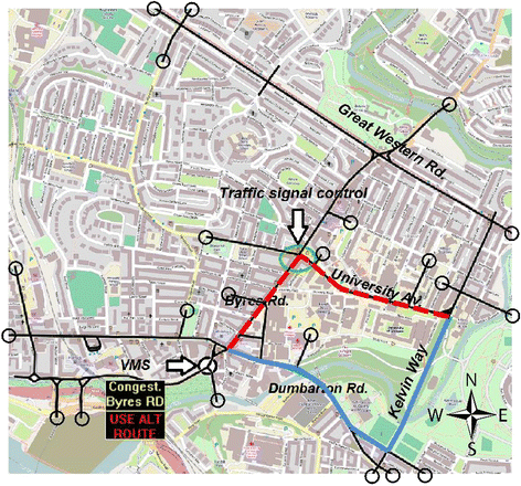
Layout of the test network (black thin line), ITS actions and key corridors
-
Variable Message Sign (VMS): the VMS is located upstream of Byres Road for those traveling from south to north, which is the main direction of travel in the morning commuting period (see Fig. 1). With text on the electronic board displayed as “Congestion on Byres Road, take alternative routes”, the VMS influences drivers’ en-route choice by diverting a portion of them to the longer yet less congested Dumbarton/Kelvinway corridor. The latter is the main alternative route to the city centre as shown in Fig. 1. Three levels of compliance rate have been considered and simulated: 10, 20 and 30 %.
-
Combination of TSC and VMS: both actions described above are implemented in the same simulation with the goal of further smoothing traffic flow on Byres Road/University Ave and reduce emissions.

The location of the ITS actions is shown with arrows in Fig. 1; the circles represent the 21 traffic zones. The main junction object of the study is indicated by the green circle. The two main corridors affected by the VMS are highlighted with red dotted lines (Byres/University Ave) and blue solid lines (Dumbarton/Kelvin) respectively.
3 Off-Line Modelling
In order to estimate the effect of the ITS actions on BC emissions a modelling tool chain has been set up (see Fig. 2). The first part of the tool chain is a microscopic traffic simulation, which provides detailed vehicle trajectories at a high time resolution (2 Hz). These data are used as input to the second part of the tool chain: the emission modelling. PM10, NOx and carbon emissions are calculated based on vehicles’ operational modes including cruising, acceleration/deceleration, and idling, which are then aggregated spatially and temporally. The third part of the procedure performs estimation of black carbon and CO2 emissions based on PM10 and carbon emissions from the previous step. The overall methodology is depicted in the flow chart in Fig. 2 together with the key input data for each module.

Overview of the methodology
A number of Key Performance Indicators (KPIs) have been identified to quantify the benefit of the proposed ITS actions:
-
Traffic perspective: travel time, vehicle speed, and delay;Footnote 1
-
Environmental perspective: black carbon, CO2, and NOx emissions.
In addition, these KPIs have been distinguished by different spatial references including junction, corridor, and network levels. Each of the proposed ITS actions has been tested using microsimulations, which are then compared with the baseline scenario (without any ITS action) in terms of all the KPIs mentioned above. The corridor and junction locations have been selected in order to cover the areas most likely affected by the proposed measures.
The remainder of this section describes in detail the three core modules of the methodology of this study.
3.1 Traffic Microsimulation
The traffic microsimulation for the test site has been developed by using S-Paramics (Sykes 2010). The setup of the model represents the scenario in 2012 for the AM peak (08:00–09:00). Due to the limited data availability for calibration it was not possible to create a baseline model for the whole day. This AM peak scenario, hereafter referred to as the base model, has been calibrated and validated using existing traffic flows from loop detectors and vehicle counts from surveys, so that simulated traffic flows are consistent with the observed traffic flows up to an acceptable tolerance. The calibration/validation has been guided by the Design Manual for Roads and Bridges (Highways Agency 2007). The goal of the calibration is to ensure that the simulated traffic has an 85 % resemblance with the actual, observed traffic in the real world within 5 GEH (GEH is a statistical formula proposed by Geoffrey E. Havers to derive the difference between observed and modelled traffic flows). The formula for GEH is shown below.
where M denotes the modelled flow and C is the observed flow.
The base model has been calibrated and validated using two data sources: manual counts and a set of inductive loop detectors. The manual vehicle counts are distinguished by vehicle type including: car/taxi, van, bus, LGV and HGV. This task has been undertaken by the Glasgow City Council and the CARBOTRAF project team. The data have been scaled in order to refer to a typical working day (Monday-Thursday) of May 2010. The detectors were available at two locations on the test site; each location is equipped with four detectors, each monitoring one lane on a two-lane, bi-directional road segment. The data have been provided for 60 days, which were further reduced to 42 days after public/school holidays were filtered. 19 out of these 42 days were used for the calibration, and the remaining was used for the model validation. The traffic volumes have been averaged across the various dates. This data together with the manual counts have allowed the generation of a “survey” file required for the matrix estimation.
It is known from literature that the road gradient plays a significant role in carbon footprint (Sobrino et al. 2014), therefore this attribute has been included in the microsimulation and emission modelling. Seven vehicle types are defined in the model and their equivalent Passenger Car Unit (PCU) are computed. The conversion to PCU is based on the Transport for London’s traffic modelling guidelines (TfL 2010). Vehicle/driver behaviour characteristics are represented by aggression and awareness factors in S-Paramics. These factors influence a driver’s gap acceptance, car following and lane changing characteristics. The default normal distribution of driver’s behaviour is assumed for the current model. The microsimulation adopts a vehicle fleet composition based on the Annual Average Daily Flow (AADF) data for Glasgow city from the Department for Transport from 2000 to 2010. The calibration results for the base model are shown in Table 1.
It is important to capture the dynamics of network traffic flows over time and space (Mahmassani 2001), therefore the dynamic assignment approach has been applied within this study. In addition, building on the base model for a period of 8–9 am, five different scenarios have been generated to take into account demand variability across different days of the week within Monday–Thursday. Based on processed historical data from the loop detectors five boundary conditions have been generated to represent demand increase from different directions into the network. Boundary conditions 1, 3 and 5 present an increase of the demand from the West and the North with different levels. While boundary conditions 2 and 4 present an increased demand from the South.
Due to the stochastic nature of the microsimulation model, each scenario has been run with 25 random seeds and the results have been averaged.
3.2 Emission Modelling
The instantaneous NOx, PM10 and total carbon emissions of each vehicle in the simulation are calculated using the AIRE (Analysis of Instantaneous Road Emissions) vehicle exhaust emission model. AIRE has been developed to use the outputs from traffic simulation models to generate vehicle emissions based on detailed dynamic data for each individual vehicle, for each simulation step (generally 2 Hz). Currently, AIRE has been specifically designed in such a way that can be used directly with S-Paramics (2011).
The combination of microsimulation traffic modelling and AIRE provides significantly more disaggregate and detailed emission estimates compared with traditional, average speed-based methods. AIRE incorporates an Instantaneous Emission Modelling (IEM) table, which is derived from PHEM (Passenger Car and Heavy Duty Emission Model) developed by the Technical University of Graz. It enables emissions to be simulated for various engine speeds and loads. The model effectively combines the PHEM emissions database and estimation methods with a development of the emissions grid methodology employed in MODEM. Local variations in fleet composition can be reflected through direct editing of the fleet composition files.
AIRE is capable of estimating NOx, particulate matter and total carbon that result from the combustion of fuel throughout each vehicle journey and can be configured to link to trajectory data from probe vehicle data collection for validation exercises. The total carbon metric is based on the PHEM fuel consumption metric and consequently can be directly converted into a representative CO2 emission.
3.3 Post-Processing Tool
As AIRE does not directly estimate the Black Carbon (BC) and CO2 emissions, a post-processing tool has been developed to provide a realistic estimation of instantaneous BC and CO2 emissions.
The Black Carbon is calculated through the COPERT IV model. Within this model, PM is apportioned between Elemental Carbon (EC) and organic mass (OM) in the emission inventory. These factors are expressed as a proportion of PM2.5 emissions. COPERT also contains emission factors representing the apportionment between PM2.5 and PM10 (the PM2.5/PM10 ratio) for different environments. These factors permit the estimation of the EC fraction of PM10 exhaust emissions. For the purposes of assessing road vehicle emissions it is also accepted that EC is effectively equivalent to BC due to the nature of the combustion processes in vehicles. This combination of assumptions and emission apportionment factors then provides a feasible methodology for estimating BC emissions within the current framework. Figure 3 illustrates this workflow.

Calculation of Black Carbon emission
The following assumptions have been made in the emission calculation.
-
The estimation of amount of CO2 generated is derived from the Total Carbon by using the atomic weights of Carbon and Oxygen to generate a factor of 44/12 (i.e. one molecule CO2 weighs 44, one atom carbon weighs 12);
-
The estimation of Black Carbon is based upon the predicted PM10 emission rates, using the COPERT IV methodology for conversion (Gkatzoflias et al. 2006);
-
The PM10 value estimated using the emission model only includes exhaust emission;
-
All exhaust PM10 ≈ PM2.5 (Gkatzoflias et al. 2006);
-
Elemental Carbon ≈ BC (Ntziachristos LaS 2013).
We note that further modelling efforts are needed to assess the pollutant concentration at various locations. These include dispersion modelling based on meteorological data such as wind direction and speed, temperature and humidity, as well as 3-D data related to building layouts, street elevations, etc. The dispersion modelling is beyond the scope of this paper.
4 Simulation Results
This section reports the simulation results for the Glasgow test site to assess the impact of the ITS actions on traffic and emissions. The results are discussed for the three ITS actions simulated:
-
Traffic Signal Control (TSC)
-
Variable Message Sign (VMS)
-
Combined TSC and VMS.
The simulation results are presented in terms of the Key Performance Indicators (KPIs) as set out in Section 3. These KPIs are calculated at junction, network and corridor levels. The two main corridors have been considered in the analysis to ensure that certain localised effects of the ITS actions were captured and they are:
-
Byres/University (indicated as dotted red line in Fig. 1)
-
Dumbarton/Kelvin (indicated as solid blue line in Fig. 1).
Due to the stochastic nature of the microsimulation model, each scenario was run with 25 random seeds and the results were statistically analysed. We then calculated the confidence interval for each indicator based on the simulation results, given the standard deviation across the 25 random seeds. In this paper we present only the simulation results that are statistically significant (i.e. with a confidence level (CL) of at least 90 %).
4.1 Overview of Results and Discussion
This section provides an overview of the results for the delay and the black carbon emissions at four different spatial references: network level, junction level, and the two aforementioned corridors. The results are shown in Figs. 4 and 5 expressed as ranges of differences (in percentage) between the ITS action case and the base case. These ranges are obtained from all five boundary conditions, each with 25 simulation runs with different random seeds. A negative sign means that the proposed ITS action reduces the relevant quantity compared to the base case; and a positive sign implies an increase.

Overview of the impact of ITS actions on delay at four spatial references. The vertical intervals refer to the changes in the ITS cases relative to the base case

Overview of the impact of ITS actions on black carbon emission at four spatial references. The vertical intervals refer to the changes in the ITS cases relative to the base case
The results show that the impact of the ITS actions varies depending on the spatial reference of the indicators: at network and corridor levels the combined ITS action TSC-VMS10 seems to bring the highest benefits in terms of delay across all spatial KPIs except at the junction. At the junction level all the VMS scenarios have seen improvements in terms of reducing delays. On the other hand, the combined TSC and VMS actions may increase the delays at the junction for certain boundary conditions (namely, 2 and 4), due to the increased red time to certain arms of the junction.
A further breakdown of the simulation results shows that the impact of the proposed actions is highly dependent on the boundary conditions (as demonstrated by the wide vertical intervals in Figs. 4 and 5) and, to a lesser extent, on the compliance rate of the VMS. Most traffic and emission improvements occur under boundary conditions 1, 3 and 5 with increased demand from the North. When the demand from the South and the West is higher (boundary conditions 2 and 4), the proposed ITS strategies do not seem to improve traffic conditions, but instead can cause substantial worsening at local levels. The black carbon emissions tend to get worse when congestion builds up under these boundary conditions. It is therefore recommended to monitor the inflows of the system in an operational environment to understand the current demand profiles before activating the ITS actions. This is addressed within CARBOTRAF by the decision support system, which determines whether or not an ITS action should be activated by the traffic operator, based on real-time data feed from the traffic sensors.
As expected, in most scenarios a reduction in traffic delay is accompanied by a reduction in BC (and CO2) emissions. However, some instances of conflicting results have also been identified. A detailed analysis at the link level reveals that a slight increase in traffic flow (and hence increased delay) does not necessarily bring more BC emissions as long as the traffic remains in the free-flow phase. This is due to the smoothing effect caused by traffic moving at a relatively uniform speed. Moreover, fleet composition also plays a vital role in the BC emissions, as some heavy goods vehicles contribute significantly to the emissions regardless of the overall traffic conditions. A detailed discussion of these issues is presented in Section 4.5.
In order to demonstrate the variability of the performance indicators (delay and BC emission) in response to the 25 random seeds, we show in Figs. 6 and 7 the box plots for all seven ITS actions under a given boundary condition.

Box plots of traffic delay at the four spatial references, under a given boundary condition

Box plots of BC emission at the fours spatial references, under a given boundary condition
We note that not all the proposed ITS actions lead to improvements at all the spatial references and for all the boundary conditions. In fact, it is entirely possible that traffic at one location is improved at the expense of worsened traffic at other locations. However, the analyses presented here are meant to provide a comprehensive picture of the aforementioned trade-offs, rather than finding an optimal solution that dominates others at every instance (such a solution is unlikely to exist). Whether a trade-off is acceptable to traffic operators is subject to further interpretation supported by the simulation results and further data; this is beyond the scope of this paper.
The following sub-sections present and discuss, in further detail, the simulation results for the three ITS actions: traffic signal control (TSC), variable message sign (VMS), and combined actions (TSC-VMS). Each ITS action is tested against all five boundary conditions; and each boundary condition was simulated using 25 random seeds.
4.2 Traffic Signal Control (TSC)
In this scenario a new traffic signal plan is proposed at the critical junction of Byres Road /University Avenue. The proposed plan keeps the existing cycle time while reducing the green time from North and West and extending the green time for the traffic approaching the junction from the South and the East. The new green times are obtained by applying the Webster formula (Webster 1958). The new signal plan maintains coordination with adjacent junction through a fixed offset.
Figure 8 and Table 2 show the layout of the core junction and the signal staging and timing plans. Compared to the base case, the proposed signal timing plan increases green times for the South and East arms and reduces green times for the North and West arms.

Schematic junction layout at Byres Road and University Avenue, and the stage diagram
The main benefit of this TSC action in terms of traffic KPIs can be noted on the Byres/University corridor for all 5 boundary conditions as the green time for the northbound has been extended (see Figs. 4 and 5 in Section 4.1.) The impact at local levels depends on the boundary condition, as can be seen from the wide range of the intervals with both positive and negative changes. Under boundary conditions 1, 3 and 5, where demand from the West or North is increased, the benefits of TSC are significant at all spatial references. The slightly reduced green time for the West arm can still accommodate the demand under boundary conditions 1, 3 and 5. Under boundary condition 2, where demand from the West is moderately increased, the proposed TSC causes minor traffic deterioration at the junction. When the demand from the West is substantially increased (boundary condition 4) the degradation on the West arm is critical and causes a reduction in speed by 23 % and an increase in delay by 33 %.
On the emission side, the overall results show a trend similar to the delays. The BC emissions are reduced on the South and East arms of the junction, which is expected due to the extended green times for those two arms. As a result, there is an improvement on both Byres/University and Dumbarton/Kelvin corridors in terms of BC emissions. Under boundary conditions 1, 3 and 5, it is observed that there is a significant reduction in NOX, CO2, and BC emissions on the network and junction levels. On the corridor level, the emission of all three pollutants is reduced on the Byres/University corridor for these boundary conditions, with a reduction by up to 8 % (BC reduction for boundary condition 1). For Dumbarton/Kelvin corridor, there is also an improvement in term of BC emission, with the maximum reduction of 5 % (boundary condition 1). Under boundary conditions 2 and 4, the emission results are mixed: while there is an improvement on the network level, minor deterioration on the junction level has been observed. This is most likely to be caused by the substantial demand increase from the West arm of the junction under these two boundary conditions.
Figure 9 shows the impact of the TSC on traffic and emissions at the network level and the junction level, under boundary condition 3. The diagrams in this figure show the improvements of the proposed TSC in terms of both traffic KPIs (travel time, speed, and delay) and environmental KPIs (NOX, CO2, and BC).

Impact of TSC on traffic and emissions under boundary condition 3
In conclusion, the TSC brings significant benefits in all spatial references (junction, corridor and network) under boundary conditions 1, 3 and 5. Under boundary conditions 2 and 4 the effects are mixed and, in particular, the improvements at some locations (e.g. the southern end of Byres Rd) outweigh the deterioration at other locations (e.g. junction and northern end of Byres Rd).
4.3 Variable Message Sign (VMS)
This section describes the simulation results for the variable message signs (VMS), which provides real-time route guidance that encourages drivers to switch from the Byres/University corridor to the Dumbarton/Kelvin corridor (see Fig. 1). As discussed at the end of Section 2, three VMS compliance rates (CR) are considered, leading to three scenarios: VMS10 (10 % CR), VMS20 (20 % CR), and VMS30 (30 % CR). These three CR have been chosen in line with the literature review (references are included section 1). The location of the VMS and the relevant routes are shown in the Fig. 1. The text displayed on the VMS is: “Congestion on Byres Road, take alternative routes”.
In order to capture the potential flow shift towards the VMS-suggested route, we first identify O-D pairs that are potentially influenced by the VMS; then we employ the path routing function embedded in S-Paramics to specify, prior to the assignment, a fixed portion (respectively 10, 20 and 30 %) of the relevant O-D demands, which will always use the alternative route through Dumbarton/Kelvin. The rest of the demands are then applied in the assignment task within the simulation. Similar to the TSC case, 5 boundary conditions are simulated for the VMS case, each with 25 random runs.
At the corridor level major effects take place on Byres Road as expected. In particular, with the exception of boundary condition 4, the simulation results for the rest of the boundary conditions and for all compliance rates show a delay reduction in the range of [3, 9 %]. Such improvements are only partially offset by worsening traffic along the alternative route (Dumbarton/Kelvin Way) where delay increases up to 2 % for all boundary conditions except 4. Figure 10 shows the simulation results for the two key corridors impacted by the VMS, under scenario VMS30 with boundary condition 1.

Impact of VMS30 on traffic and emissions under boundary condition 1
The results with boundary condition 4 differ from the other boundary conditions as the simulation shows a substantial worsening of traffic conditions at the corridor and network levels. This is explained by the fact that the increased demand from the South under this boundary condition causes substantial delay on the Kelvin Way (480 s on average). This congestion is aggravated by the additional vehicles shifted to this corridor due to the VMS. For example, in the VMS30 case there is an increase in delay by 20 % on the Dumbarton/Kelvin corridor.
The VMS action brings significant reduction in delay under boundary conditions 1, 3 and 5 by up to 9 % on the Byres/University corridor, and up to 3 % at the network level. Such improvements, however, are highly dependent on the both boundary condition and the compliance rates. On the emission side, the VMS actions bring a relatively small improvement on black carbon emissions for boundary condition 1, 3 and 5, in the range of 0 to 2 % (network level). Under boundary conditions 2 and 4, the results on emission are mixed. No significant improvements are observed on the network level. However, on the junction level, there is a slightly improvement of BC emission, by up to 3 % reduction. On the corridor level, while there is a reduction BC emission for Dumbarton/Kelvin corridor, there is an increase of emissions on Byres road and University Avenue.
4.4 Combined TSC-VMS
This section provides an overview of the results of the simulation for the scenario TSC-VMS where both the new traffic signal control at the Byres/University junction and the VMS at various compliance rates (10/20/30 %) are simulated at the same time. Five boundary conditions are simulated, each with 25 random runs.
At the network-wide level the combination measures of TSC and VMS bring traffic improvement for all boundary conditions and compliance rates with a reduction in delay ranging in [3, 6 %]. The combined strategy always brings substantial traffic improvement for the Byres/University corridor for all boundary conditions and compliance rates; in particular, overall the simulation has seen an increase in vehicle speeds by [19, 24 %], and a reduction in delay by [21, 29 %]. However, these benefits are partially offset by increased delay by (1) up to 8 % along the VMS-suggested Dumbarton/Kelvin corridor under boundary conditions 1, 2 and 4; and (2) up to 36 % increase at the Byres/University junction under boundary conditions 2 and 4, mainly due to the reduced green time in TSC on the West arm of the junction.
In this combined strategy, a significant re-distribution of flow is observed. The increased green time allocated to the East arm of the junction, combined with the VMS re-routing action, lead to a shift of flow from Byres Road to Dumbarton Road/Kelvin Way. This results in an improvement in traffic KPIs on Byres Road.
The combined strategy leads to a substantial reduction in BC emissions on Byres Road and University Avenue, namely between 2 and 11 % across all different boundary conditions. However, this is offset by increased emissions on the alternative route Dumbarton/Kelvin corridor except in boundary condition 4, where interestingly a reduction in NOx and BC is also observed (see section 4.5 for more analysis of this case). Overall the improvement outweighs the deterioration, and as a result the combined ITS action leads to a change in black carbon emission ranging from −3 to 1 % at the network level. Figure 11 shows the traffic and emission KPIs for the combined ITS action under boundary condition 4 for the two corridors.

Impact of TSC_VMS30 on traffic and emissions under boundary condition 4
While the results along Byres/University corridor show that traffic and emission KPIs improved simultaneously, the results on the Dumbarton/Kelvin corridor suggest a trade-off between the two. The next section provides a more detailed description of such a conflicting result, along with some analysis.
4.5 Factors Influencing Emissions
In this section we look further in detail into possible factors that influence vehicle emissions: 1) speed homogeneity and 2) fleet composition. These two factors will be illustrated using one example from our simulation. In particular, we consider the simulation of VMS30 under boundary condition 1, as shown in Fig. 10.
-
1)
Speed homogeneity. On the Dumbarton/Kelvin corridor an increased congestion is seen, which is expected since traffic are diverted to this corridor due to the VMS. However, both NOx and BC emissions are reduced, indicating potential conflict between traffic and environmental KPIs. Further investigation of these results at a refined and microscopic level within the corridor (Table 3) shows that the standard deviation of vehicle speeds is lower in the ITS scenario. Detailed link-specific data are reported in Table 3. It can be seen that, although re-routing some vehicles leads to a minor increase in delay on the alternative route, traffic becomes more smoothed on this route due to a more homogeneous driving condition, which is likely to be caused by the slightly increased vehicle. As a consequence, the vehicle speed has less variation in the ITS case, leading to less BC emissions.
Table 3 Link analysis speed variability in the base case and the ITS case (VMS30) under boundary condition 1 -
2)
Fleet composition. We have also analysed the driving characteristics per vehicle type on the link with the highest BC reduction: 377:372. Table 4 reports some quantities related to traffic and emissions for the base scenario on this link. In this table, count of acceleration and count of deceleration are obtained in the following way: for a given vehicle we count the number of time instances at which it was accelerating or decelerating; these counts are then summed over all vehicles of the same type that traversed this link within the 1-h simulation period. One immediately observes from Table 4 that buses have the highest contributions to the BC emissions on this link, despite the fact that their flows are substantially lower than other types of vehicles: they actually contribute to more than half of the total BC emissions on this link even if they represent only 3 % of the total flow on the link. Similar results have been founds for the adjacent links as shown in Table 4.
Table 4 Key indicators for traffic and emissions for the base scenario, boundary condition 1 at link level
This section analyses the impacts of speed homogeneity and fleet composition on road emission. The speed variation is one major source of emission, as it not only causes more acceleration and deceleration but also triggers complex waves such as stop-and-go waves and phantom jam, which hold responsibility for even more emissions. On the other hand, the significant contribution of buses or HGVs to emissions as demonstrated in the simulations necessitates explicit modelling of fleet composition within microsimulation, or a thorough calibration procedure in mesoscopic/macroscopic modelling, which tends to ignore such information.
5 Conclusions and Future Research
This paper presents the microsimulation results from the CARBOTRAF project, which aims to provide adaptive traffic management to reduce CO2 and black carbon emissions. The simulation study is conducted for a test network in Glasgow, with 5 different demand levels considered to account for daily variability of the traffic conditions. Three different traffic management measures are considered: traffic signal control (TSC), variable message sign (VMS), and the combined TSC and VMS. The simulation results have demonstrated the effectiveness of these actions in reducing BC emissions and improving traffic conditions. However, these benefits depend on a number of factors such as the demand level and the VMS compliance rate. With regards to the first factor, the proposed study considers a relatively coarse variation of the initial demand through the five boundary conditions. The results show indeed that the impact can be either positive or negative depending on the boundary condition. It would be beneficial to investigate this further through a more fine variation of the demand to provide more generalised results about the benefits achievable through these interventions.
The results are also sensitive to the VMS compliance rate. This has been considered here as an exogenous variable. However, a more accurate estimate of the ITS actions’ impact would benefit from a better estimate of the compliance rate. Further research will entail modelling the compliance rate as an endogenous variable to study its interaction with the traffic flows across the network.
A detailed analysis of BC emissions per vehicle type demonstrates the high contribution of buses to the overall emissions. Results indicate that that a bus flow as low as 17v/h equivalent of 5 % of the total flow, is responsible for 71 % of the overall BC emissions on the link. This suggests that other types of interventions targeting specific types of vehicles may be more effective than the ITS actions studied in this research in reducing BC emissions.
The simulation results reveal the likely trade-off between traffic/environmental KPIs at different locations in the network. For example, the re-routed traffic, as result of the VMS, tends to alleviate the congestion and the emissions on the main corridor at the expense of the alternative route. Such a trade-off is sometimes necessary as those congestion externalities can be shifted spatially to less populated areas to yield less impact on public health. In addition, the results suggest the potential conflict between traffic KPIs and environmental KPIs (see, for example, section 4.5), which should be further investigated to shed light on the complex decision context when managing urban traffic.
Notes
Here in this paper, delay represents the difference between the experienced travel time and the free-flow travel time.
References
Barnes J, Paruchuri V (eds) (2012) Optimal phase ordering of traffic signals to reduce stopped delay. Advanced Information Networking and Applications (AINA), 2012 I.E. 26th International Conference on; 2012 26–29 March
Brocken MGM, Van der Vlist MJM (eds) (1991) Traffic control with variable message signs. Vehicle Navigation and Information Systems Conference, 1991; 1991 20–23 Oct
Chatterjee K, Hounsell NB, Firmin PE, Bonsall PW (2002) Driver response to variable message sign information in London. Transp Res C Emerg Technol 10(2):149–169
Chen K, Yu L (2007) Microscopic traffic-emission simulation and case study for evaluation of traffic control strategies. J Transp Syst Eng Inf Technol 7(1):93–100
Chen SLM, Gao L, Meng C, Li W, Zheng J (eds) (2008) Effects of Variable Message Signs (VMS) for improving congestions. International Workshop on Modelling, Simulation and Optimization
Cummings M (ed) (1994) Electronic sign strategies and their benefits. Road Traffic Monitoring and Control, 1994, Seventh International Conference on; 1994 26–28 Apr
De Coensel B, Can A, Degraeuwe B, De Vlieger I, Botteldooren D (2012) Effects of traffic signal coordination on noise and air pollutant emissions. Environ Model Softw 35:74–83
Dia H, Cottman N (eds) (2006) Modelling the environmental benefits of its using power-based vehicle emissions models. 13th ITS World Congress. London
Erke A, Sagberg F, Hagman R (2007) Effects of route guidance variable message signs (VMS) on driver behaviour. Transport Res F: Traffic Psychol Behav 10(6):447–457
Gkatzoflias D, Kouridis C, Ntziachristos L, Samaras Z (2006) COPERT 4 manual. European Environment Agency (EEA)
Han K, Liu H, Gayah V, Friesz TL, Yao T (2015) A robust optimization approach for dynamic traffic signal control with emission considerations. Transportation Research Part C. doi:10.1016/j.trc.2015.04.001
Highways Agency (2007) Design manual for roads and bridges. H.M.S.O, London
Hoye A, Sorensen M, Elvik R, Akhtar J, Navestad T, Vaa T (2011) Evaluation of variable message signs in Trondheim. Norwegian Centre for Transport Research. Report 1153/2011
Janssen NAH, Gerlofs-Nijland ME, Lanki T, Salonen RO, Cassee F, Hoek G, Fischer P, Brunekreef B, Krzyzanowski M (2013) Health effects of black carbon. In: Europe WROf (ed)
Kattan L, Habib KMN, Tazul I, Shahid N (2011) Information provision and driver compliance to advanced traveller information system application: case study on the interaction between variable message sign and other sources of traffic updates in Calgary, Canada. Can J Civil Eng 38(12):1335–1346
Kickhöfer B, Nagel K (2013) Towards high-resolution first-best air pollution tolls. Netw Spat Econ 1–24
Kottapalli A, Mahmassani H, Bhat C, Ridge O (2003) Intelligent transportation systems and the environment. Center for Transportation Research, Austin
Lam WHK, Chan KS (eds) (1991) A stochastic traffic assignment model for road network with travel time information via variable message signs. Conference on Intelligent Vehicles
Lee C, Choi K, Lee S (2004) Evaluation of drivers’ responses to ATIS: a practical VMS based analysis. KSCE J Civ Eng 8(2):233–237
Li X, Li G, Pang S-S, Yang X, Tian J (2004) Signal timing of intersections using integrated optimization of traffic quality, emissions and fuel consumption: a note. Transp Res Part D: Transp Environ 9(5):401–407
Li J-Q, Wu G, Zou N (2011) Investigation of the impacts of signal timing on vehicle emissions at an isolated intersection. Transp Res Part D: Transp Environ 16(5):409–414
Lin X, Tampère CMJ, Viti F, Immers B (2014) The cost of environmental constraints in traffic networks: assessing the loss of optimality. Netw Spat Econ 1–21
Lv J, Zhang Y (2012) Effect of signal coordination on traffic emission. Transp Res Part D: Transp Environ 17(2):149–153
Maheshwari P, Khaddar R, Kachroo P, Paz A (2014) Dynamic modeling of performance indices for planning of sustainable transportation systems. Netw Spat Econ 1–23
Mahmassani H (2001) Dynamic network traffic assignment and simulation methodology for advanced system management applications. Netw Spat Econ 1(3–4):267–292
Mammar S, Haj-Salem H, Messmer A, Papageorgiou M, Jensen L (eds) (1996) VMS information and guidance control strategies in Aalborg. Vehicle Navigation and Information Systems Conference, 1996 VNIS '96; 1996 14–18 Oct
Ntziachristos LaS Z (2013) EMEP/EEA air pollutant emission inventory guidebook. 12/2013
Ramanathan V, Carmichael G (2008) Global and regional climate changes due to black carbon. Nat Geosci 1(4):221–227
Ramsey ED, Luk J (1997) Route choice under two australian travel information systems. ARRB Transport Research
Schlaich J (2010) Analyzing route choice behavior with mobile phone trajectories. transportation research record. J Transp Res Board 2157(−1):78–85
Sharma S (2010) An analysis of black carbon and health effects
Sobrino N, Monzon A, Hernandez S (2014) Reduced carbon and energy footprint in highway operations: the Highway Energy Assessment (HERA) methodology. Netw Spat Econ 1–20
S-Paramics (2011) S-Paramics 2011 reference manual. SIAS limited, Edinburg
Sykes P (2010) Traffic simulation with paramics. In: Barceló J (ed) Fundamentals of traffic simulation. Springer, New York, pp 131–171
TfL (2010) Traffic modelling guidelines: TfL traffic manageer and network performance best practice. Transport for London
UNEP (2011) Integrated assessment of black carbon and troposhperic ozone: summary for decision makers
United States Environmental Protection Agency (2012) Black carbon health effects. Available from: http://www.epa.gov/airscience/air-blackcarbon.htm
United States Environmental Protection Agency USEPA (2013) Causes of climate change. Available from: http://www.epa.gov/climatechange/science/causes.html
U.S. Environmental Protection Agency (2012) Report to Congress on Black Carbon. Department of the Interior, Environment, and Related Agencies Appropriations Act. EPA-450/R-12-001
Webster FV (1958) Traffic signal settings. H.M.S.O., London
Wei S, Wu J, Shaolin Z, Ling Z, Zhi T, Yu Yu Y et al (2009) Variable message sign and dynamic regional traffic guidance. Intell Transp Syst Mag IEEE 1(3):15–21
Zhang Y, Chen X, Zhang X, Song G, Hao Y, Yu L (2009) Assessing effect of traffic signal control strategies on vehicle emissions. J Transp Syst Eng Inf Technol 9(1):150–155
Zhao D, Shao C (eds) (2010) Empirical study of drivers’ learning behavior and reliance on VMS. 2010 13th International IEEE Conference on Intelligent Transportation Systems (ITSC); 2010 19–22 Sept
Acknowledgments
This study has been undertaken within the CARBOTRAF project funded by the EU 7th Framework Program under grant agreement n° 28786. We would like to express our deep gratitude to Mr Jim Mills at Air Monitors and Mr Brian Davidson in Glasgow City Council, for their generous support throughout the project and provision of relevant data.
Author information
Authors and Affiliations
Corresponding author
Rights and permissions
Open Access This article is distributed under the terms of the Creative Commons Attribution 4.0 International License (http://creativecommons.org/licenses/by/4.0/), which permits unrestricted use, distribution, and reproduction in any medium, provided you give appropriate credit to the original author(s) and the source, provide a link to the Creative Commons license, and indicate if changes were made.
About this article

Cite this article
Mascia, M., Hu, S., Han, K. et al. Impact of Traffic Management on Black Carbon Emissions: a Microsimulation Study. Netw Spat Econ 17, 269–291 (2017). https://doi.org/10.1007/s11067-016-9326-x
Published:
Issue Date:
DOI: https://doi.org/10.1007/s11067-016-9326-x