Motion dense sampling and component clustering for action recognition

Abstract

In this paper, we propose Motion Dense Sampling (MDS) for action recognition, which detects very informative interest points from video frames. MDS has three advantages compared to other existing methods. The first advantage is that MDS detects only interest points which belong to action regions of all regions of a video frame. The second one is that it can detect the constant number of points even when the size of action region in an image drastically changes. The Third one is that MDS enables to describe scale invariant features by computing sampling scale for each frame based on the size of action regions. Thus, our method detects much more informative interest points from videos unlike other methods. We also propose Category Clustering and Component Clustering, which generate the very effective codebook for action recognition. Experimental results show a significant improvement over existing methods on YouTube dataset. Our method achieves 87.5 % accuracy for video classification by using only one descriptor.

1 Introduction

In recent years, the number of videos is explosively increasing. To handle these videos, action recognition is paid highly attention to, and a lot of action classification methods have been proposed and developed in the past few decades. The framework based on a machine learning method (such as SVM) with Bag-of-features(BoF) representation is most widely used for this purpose. This is because this framework shows high performance even for difficult conditions such as significant intra-class variation, occlusion and background clutter. However, there remain a lot of questions to construct a high-performance system by using this framework. For example, nobody knows which interest point detection method should be used and/or which feature descriptor should be used etc. This paper focuses on answering the two questions as shown in Fig. 1. The first question is how to develop an effective interest point detection method. And the second question is how to generate effective codebook. Today, SIFT [14]/SURF [1] or dense sampling are widely used for still image classification as an interest point detection and a feature descriptor. And spatiotemporal interest points(STIP) [2, 6] or dense trajectory (DT) [21] are used for video classification in most cases. However, few researchers doubt this is true. Also, very simple methods such as K-means [10] are used for clustering. Few researchers also doubt this is true.

Fig. 1

The typical framework of BoF and SVM. Square object denote the process, and ellipse denote the document. This paper focuses on the processes which is indicated by blue

Under this situation, we propose two methods in this paper. The first proposal is a new interest point detection method which detects more informative interest points from video frames based on dense sampling strategy called “Motion Dense Sampling” (MDS). The advantage of MDS is that it detects only interest points which belong to action region of all regions of a video frame regardless of the size of action regions in a video frame. Also, MDS extracts scale-invariant features from a video frame. The second proposal is a new clustering method which generates more efficient codebook than traditional methods called “Component Clustering”.

The rest of this paper is as follows. We describe related work in Section 2. In Section 3, we propose MDS and describes the details of MDS. In Section 4, we propose Component Clustering and describe them in detail. In Section 5 we show the experimental results and evaluate our proposals. Finally we wrap up with this paper in Section 6.

2 Related work

Action recognition is one of the most active research topics in computer vision over the recent years. Liu et al. [13] have proposed the method to use Harris-Laplacian (HAR), Hessian-Laplacian(HES) and MSER detector [17] in order to detect the interest points. Then they employed SIFT [14] as a feature descriptor. They also employed STIP proposed by Dollar et al. [6] for motion features. Furthermore they also employed HoF [12] as a feature descriptor. Ikizler et al. [11] have proposed the method to extract features from moving human regions, important objects and overall properties of the frame separately. They employed the tracking-by-detection method, which includes the tracking method proposed by Felzenswalb et al [9] and mean-shift tracking method [3]. Also, they are using different interest point detection and feature descriptor for each regions. Finally, they classified data by combining the features from each regions.

Wang et al. [21] have proposed DT which uses the dense optical flow computed by Farneback algorithm [7] to detect interest points and to describe motion features [15, 16]. They employed HOG [4], HOF, and MBH [5] as a descriptor. After generate these features, they combined them by multi-channel approach [20]. As is clear from the above researches, most of existing systems employed STIP or DT to detect interest points. In these systems, a single fixed value or a few fixed values are typically used for the scales of feature description. However, past studies [8, 19] show non-grid interest points are not always effective for classification. And they also show the fixed scale does not achieve good results for the scale invariance. But, as long as authors know, there are very few studies to try to solve these problems. Another problems of existing systems are using simple clustering methods such as K-means. We guess many researchers in this field do not think that a clustering method is an important factor for the performance and/or that there is no room to improve it. However, these assumptions are not correct as shown in Section 4.

3 Motion dense sampling

In this section we propose MDS and the framework for an action recognition system using MDS. MDS has three advantages compared to other existing methods as follows. Because of these advantages, MDS detects very informative interest points.

• 1. MDS separates action regions from each video frames, and the separation is tough for camera motion noise.

• 2. MDS detects the ample number of interest points from only action region even if the size of action regions drastically changes.

• 3. MDS extracts scale invariant features from video frames.

The flow chart of MDS process is shown in Fig. 2.

Fig. 2

The image of MDS flow chart

3.1 Separation of action region from video frames

In this section, we discuss how to separate action region and background region based on motion information. In general, features from background region do not contribute classification results. On the contrary, they may bring harmful effects to classification results. So, we separate action region (foreground region) from video frames. The features extracted from foreground region are informative for action recognition. In order to achieve the separation, Motion Mask (MM) is automatically generated in our method. Our assumption is that actors are on a foreground region in most cases if the size of the region is large to some extent. Detection of a foreground region is done based on optical flow information. To generate MM, we decide how many successive optical flow frames should be used first. But, it is not easy to optimize. If we use a lot of optical flow frames to extract a foreground region, more reliable mask image may be generated. On the contrary, they may contain huge noise in it such as camera motion, camera shake or scene change. They may extremely degrade the separation performance. As a result, we designed to generate one MM by utilizing three basic masks generated from four video frames. Although we generate MMs by superimposing three basic masks simply, we get rid of the noisy frames and utilize only rest frames if heavy noise is contained in these frames, This provides tolerance against camera motion and enhances classification accuracy.

3.1.1 Generation of motion mask

MM is generated by the following steps.

• 1. Extract four frames from a video.

• 2. Compute optical flow by Farneback algorithm [7] between succesive two frames.

• 3. Genarate Base Mask based on optical flow information computed step 2.

• 4. Discard the Base Mask which contains heavy camera motion noise. How to judge whether discarding Base mask is discarded or not is described later (Section 3.1.2 Discarding noisy frame).

• 5. Generate MM after detecting outlier areas and eliminating them. Figure 3 illustrates these processes. And the examples of MM generation processes are shown in Figs. 4 and 5.

  Fig. 3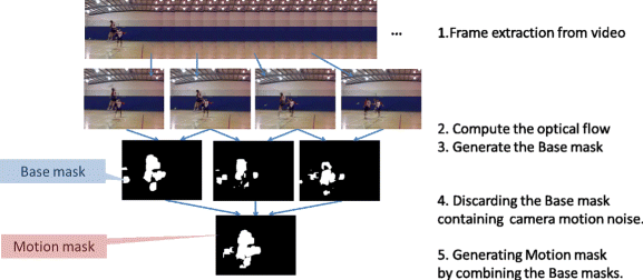

  

  The image of the Motion mask generation process

  Fig. 4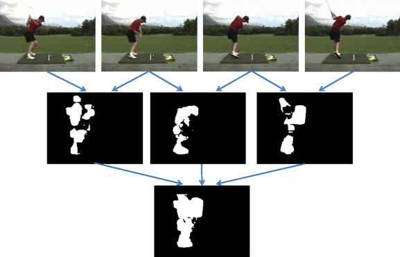

  

  The example of Motion mask generation process 1

  Fig. 5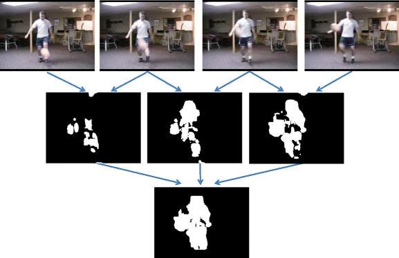

  

  The example of Motion mask generation process 2

The image of these conducts are shown in Fig. 3. And the examples of the Motion mask generation process are shown in Figs. 4 and 5.

3.1.2 Discarding noisy frame

Detection of noisy frame

We discuss how to discard Base Mask which contains heavy camera motion noise. We call such frame as noisy frame in this paper. The examples of a good mask and a noisy mask are shown in Figs. 6 and 7. As is clear in Figs. 6 and 7, the size of foreground region in a noisy frame is extremely large compared to normal Base Masks. So, we can easily detect the noisy frame using this feature. Concretely, If the size of a mask region is larger than threshold (currently we defined it as 15,000 pixels), we discard its frame by judging ”noisy frame”.

Fig. 6

The example of the noisy frame

Fig. 7

The example of the Base mask not contains the camera motion noise

Discard noisy frame

If one or two of three masks contain(s) heavy camera motion noise, we discard these masks and generate Motion mask by combining only the rest masks. But, if all masks contain camera motion noise, how to discard noisy masks depends on whether a video fully contains camera motion noise or not. If a video partly contains camera motion noise, we discard all noisy masks in process. Although, in this case, we can’t extract any information from these masks, we can detect informative interest points and extract good features from another masks. On the other hand, if a video fully contains camera motion noise, we can’t extract features from other masks. In this case, we don’t discard the third Base mask even if it contains heavy noise and generate a MM using this Base Mask. In this case, accuracy of separation of foreground region from background region is relatively low, but it is still better than detecting interest points without separation. We show three discarding schemes in Figs. 8, 9 and 10.

Fig. 8

Case1: one of three masks contains heavy noise

Fig. 9

Case2: two of three masks contains heavy noise

Fig. 10

Case3: all masks contains heavy noise and the video fully contains the camera motion noise

3.1.3 Detecting outlier areas

The target of MDS is unconstrained videos. Such videos contain noise by low resolution and/or background moving. Optical flow information generated from such noise may generate interest points from background region. This may result in lower accuracy. In this section, we discuss how to get rid of such noise. The examples of noise are shown in Fig. 11. In Fig. 11, noise is clipped by red circle. These noisy spots are likely to be small compared to normal MM generated by human action. So, we are able to get rid of these noise by this feature. To detect the noise, we generate Motion Map which shows the regional size of MMs. Motion Map is generated by counting the number of optical flow vectors around the focused pixel. The example of how to generate Motion Map is shown in Fig. 12.

Fig. 11

The example of the noises hinge on low image quality or bachground moving

Fig. 12

The example of Motion map generation

Next, by using the pixel value P(x, y) of a Motion Map, we compute average μ , and root-mean-square deviation σ. Then we get rid of the pixels which satisfy the following condition.

$$ P(x,y) < \mu - 2\sigma $$

(1)

The examples of the result is shown in Figs. 13 and 14.

Fig. 13

The example of the outlier area 1

Fig. 14

The example of the outlier area 2

3.2 Detection of the ample number of grid interest points

In this section, we discuss how to detect the ample number of interest points regardless of huge changes of the size of action region (foreground region). The homogeneity of the number of interest points detected from video frames result in high accuracy of classification. Our interest point detection method is based on dense sampling. But, if we employ normal dense sampling for interest point detection, the number of interest points changes in proportion to the size of action region. That is because normal dense sampling assumes that frame size is stable. For this reason, it employs the fixed value for sampling interval. However, it does not work well in our system because our method assumes that only foreground regions are used. The size of these regions dynamically changes. That is why we solve this problem by computing sampling interval for each frames. Our method enables to detect the ample number of interest points regardless of the size of foreground region of an image. This realizes grid based interest point detection, which is well known that more effective for classification than non-grid, and constant number of interest points at the same time. The interest points detected by our method strongly informative for classification. Unlike normal dense sampling using fixed value of sampling interval, we decide the number of interest points we want to detect from each frames in our method.

Now we denote the size of foreground region, sampling interval as S _f , I _s respectively. When we want to acquire N _f features from each frames, I _s is calculated as follows.

$$ I_s = \sqrt{\frac{S_f}{N_f}} $$

(2)

The value of S _f changes drastically for each frames, and N _f is the fixed value. If I _s is smaller than 1.0, we skip to extract features from this three-frames set. This means that the bigger Motion mask generates bigger sampling interval. The examples of sampling interval calculation is shown in Figs. 15 and 16. Figures 15 and 16 contain three pictures, in which the left one is an input frame, the central one is a MM with interest points, and the right one is an input frame with the interest points.

Fig. 15

S _f =5828, I _s =5

Fig. 16

S _f =3003, I _s =3

3.3 Extraction of scale invariant features

In this section, we discuss how to extract scale invariant features from video frames. The scale invariance is very important for classification to recognize the same object in different scales. When two actions are completely the same but the sizes of actors are different, the system has to judge ”they are the same actions”. It is impossible without any tolerance for scale invariance. However very few researches focus on this point. Some of them employ several fixed values for scale invariance. Although, this may result in extracting features by the optimal scale, this also extracts a lot of noise. In our method, we employ the variable scale value for feature extraction calculated by the size of foreground region. The size of foreground region is approximately proportional to the size of the moving person. For this reason, we can calculate the optimal scale for feature extraction by using the size of foreground region. Here, we define two kind of sampling scales. The first one aims at extracting features from only one person. We call this scale as a local scale. The other one aims at extracting features from several persons. This is useful for classifying team sports etc. We call this scale as a global scale. The difference between local scale and global scale is the size of scope to compute. Global scale is calculated by the size of MM for the whole frame. On the other hand, local scale is calculated by the size of MM for the size of the foreground region around the interest point in process.

Now, we denote the size of action region, the size of action region in the regional area of the frame, local scale, global scale as S _f , S _{f r} , S _l and S _g respectively. We also denote the maximum value of the size of action region, the maximum value of the size of action region in the regional area of the frame as S _{f m a x} , S _{f r m a x} respectively. And the minimum value of local scale, and the additional value for local scale, the minimum value of global scale, and the additional value of global scale as S _{l m i n} , S _{l a d d} , S _{g m i n} and S _{g a d d} respectively.

S _l and S _g are calculated by the following equation. S _l is calculated for each interest points and S _g is calculated for each frames.

$$ S_l = S_{lmin} + S_{ladd}\frac{S_{fr}}{S_{frmax}} $$

(3)

$$ S_g = S_{gmin} + S_{gadd}\frac{S_{f}}{S_{fmax}} $$

(4)

The value of both scale is no fewer than S _{m i n} , nor more than S _{m i n} +S _{a d d} . We use the fixed values based on our experience for S _{m i n} and S _{a d d} . By this, the bigger action region result in bigger scale. The examples of the calculation is shown in Figs. 17 and 18.

Fig. 17

The example of the local scale. left: video frame, center: Motion map, right: video frame with circles illustrated by scale size

Fig. 18

The example of the global scale. left: video frame, center: Motion map, right: video frame with circles illustrated by scale size

4 Category clustering and component clustering

In this section, we propose two new clustering methods called Category Clustering and Component Clustering. Category Clustering is a clustering method aiming at what to cluster. On the other hand, Component Clustering is a clustering method aiming at how to cluster the mass of features.

4.1 Category clustering

In most systems, features extracted from all categories are mixed and generated a mass of features. Then the clustering process is done by simple K-means algorithm [10]. On the contrary, this clustering method defines a codeword as a centroid of characteristic features appeared in each category. Unlike traditional methods, Category Clustering clusters video frames using features extracted from each category. Figure 19 shows the difference between traditional clustering method and Category Clustering. We call the codebook generated from each category as a small codebook in this paper.

Fig. 19

The image of Category Clustering

4.2 Component clustering

Component Clustering has two different characteristics from traditional clustering methods. The first characteristic is that Component Clustering doesn’t use the features at the edge of the feature space to generate codebook. It is because we can assume the clusters generated by such a few features are not informative for classification.

The second one is that it generates a codebook taking the characteristics of action recognition into consideration. Action recognition is a task to classify human actions. So, dense features for human actions are required but sparse features are enough for other scenes. For example, owing to distinguish between ”A person who is sitting” and ”A person who is standing”, we should prepare dense features even if the difference between these two scenes is very small. As a result, we have to do clustering process with variable-granularity function. Figure 20 shows the example of variable-granularity clustering.

Fig. 20

The image of the variable-granularity clustering

For the purpose of realizing this function, we should divide similar features situated closely in a feature space into optimal-size groups (= codeword). Our approach is to divide densely-distributed features into smaller groups, which is almost the same size as sparsely-distributed features. To achieve such division, Component Clustering checks the number of features belonging to each groups, and adjust to the number of features in one group. Namely, if the number of features in a group is much bigger than those in another group, this group is divided into two or more small groups. In other words, this process generates the same-size groups regardless of granularity (densely-distributed features or sparsely distributed features). In addition, if the number of features in a group is very few, the group is probably made by features at the edge of a feature space. In this case, we get rid of them soon.

To make up the number of features in each groups, Component Clustering, employs K-means clustering method with a hierarchical way. The steps of this clustering process is as follows. Here, C _i denotes the number of features in the i-th group (the i-th codeword). Also, F and C denote the number of all features in a codebook and the number of codebooks respectively. And C _{n u m} denote the ideal number of features in a group. C _{n u m} is calculated by F/C.

• 1. The number of division for a cluster D is calculated by C _i /C _{n u m}

• 2. To divide this cluster for the number of K-means method

• 3. Sorting the subclusters generated by step 2 based on the number of feaures in each subclusters.

Then, for each subclusters, judge whether this subcluster should be divided or not by the following criteria.

• C _i ≥2C _{n u m} To divide the cluster more

• 0.3C _{n u m} < C _i < 2 C _{n u m} use the cluster as a Codeword

• C _i ≤0.3C _{n u m} Discard the cluster because it is regarded as an edge cluster

To divide all clusters by the above algorithm, a very informative codebook is generated. Figure 21 shows the flow chart of this process. Also, Fig. 22 shows the distribution of the number of features in each codewords by our experiment. Blue columns in Fig. 22 shows the result of traditional clustering method and red columns shows the result of Component Clustering. As is clear in Fig. 22, we conclude Component Clustering achieves our goal that we make up the number of feature in each codewords.

Fig. 21

The flowchart of the Compornent clustering

Fig. 22

Distribution of the number of features in each clusters by our experiment

5 Performance evaluation

In this section, we present some evaluation results for our proposal. We evaluate our systems by using publicly available standard action dataset: Youtube dataset.

5.1 Experimental Condition

5.1.1 Data set

We have done some experiments for evaluating the classification performance of MDS. We used YouTube dataset [13] for our evaluation. This dataset contains 1168 videos from 11 different classes (basketball shooting, biking/ cycling, diving, golf swinging, horseback riding, soccer juggling, tennis swinging, swinging, trampoline jumping, volley ball spiking, and walking with a dog). It is well known as one of the challenging datasets for classification due to the presence of significant camera motion, large variations in object appearance and pose, object scale, viewpoint, cluttered background and illumination conditions etc. Videos for each classes are divided into 25 folds based on the similarity of actors, backgrounds, and viewpoints. We follow the original setup [13] using leaveone-out-cross validation for a pre-defined set of 25 folds. Average accuracy over all classes is reported as performance measure. Sample frames are illustrated in Fig. 23.

Fig. 23

Sample frames from video sequences on Youtube dataset. This is one of the challenging dataset due to the large variations in camera motion

5.1.2 Parameter setting of the proposed method

Codebook generation

To generate a codebook, we first detected the 300 interest points from each Motion Masks (MMs) using the method described in subsection 3.1. Then we extracted two scales (global scale and local scale) of features from each interest points described in subsection 3.2. Also, we employed SURF as a feature descriptor. After that, Component Clustering has been done for all movies in each categories which is described in subsection 4.2 due to generate smaller codebooks for each categories. In our experiment, we generated 900 codewords per one category. In consequence, the number of all codewords of a codebook is 9900 (because YouTube dataset contains 11 categories). The codebook is generated by connecting small codebooks for each categories.

BoF histogram generation and classification

To generate the BoF histogram, we detected the 300 interest points from each Motion Masks (MMs) using the method described in subsection 3.1. Then we extracted two scales (global scale and local scale) of features from each interest points described in subsection 3.2. Also, we employed SURF as a feature descriptor. The extraction of interest points and features is the same way as “Codebook generation”. After we extract featutes, descriptors are assigned to the closest codeword using Euclidean distance. And we computed the average number of features assigned to the same codeword for successive 10 frames as a BoF histogram. We generated the 50 BoF histograms from each movies. For better classification we used a non-linear SVM with RBF kernel. The default values are used for γ(=1.0) and C (=1.0) in RBF. The movie was classified the category which the number of BoF histogram generated from the movie in process classified was the largest.

5.2 Experimental results and evaluation

Table 1 shows the experimental result for YouTube dataset, in which the proposed method is compared to Ikizler [11], Wang [21] and Nagendar [18]. As is clear in Table 1, our method has achieved classification accuracy of 87.5 % on average. Furthermore, our method uses only one descriptor as described in Section 3 while the other methods employ 4 or 5 descriptors like HOG, HOF, MBH and SIFT etc. This indicates our descriptor is more excellent than the other descriptors in terms of discriminative power.

Table 1 Accuracy per descriptor for the YouTube dataset. we compare with Ikizler [11], Wang [21], Nagendar [18] (There isn’t the data of accuracy by single descriptor). Our method achive the best accuracy

6 Conclusions

In this paper, we proposed Motion Dense Sampling (MDS), which detects very informative interest points from videos. And we also proposed two clustering method, which generate very informative codebook for action recognition. According to our experimental results, the proposed method shows video classification accuracy of 87.5 % for YouTube dataset. This is better score than any other exiting methods.

There are at least three contribution of this paper. Firstly, we showed our method can easily distinguish foreground region from background regions by using motion information even when videos contain some harmful conditions such as camera motions etc. It must be useful to improve the performance of video classification. Secondly, we proved by our experiment that the combination with multiple local features does not always show the best performance. It is clear by the fact that our single descriptor shows higher performance than the other methods based on multiple descriptors. Thirdly, we showed that Category Clustering and Component Clustering are highly effective to accuracy of classification. The remaining issue is that to generate more reliable Motion mask utilizing the consecutiveness of the position of the actors in the video. Also to add the new process in the case of the video fully contains the camera motion is the future work.

References

Bay H, Tuytelaars T, Van Gool L (2006) Surf: speeded up robust features. In: Computer vision-ECCV 2006. Springer, pp 404–417
Bregonzio M, Shaogang G, Tao X (2009) Recognising action as clouds of space-time interest points. In: IEEE conference on computer vision and pattern recognition (CVPR), pp 1948–1955
Comaniciu D, Ramesh V, Meer P (2003) Kernel-based object tracking. In: IEEE transactions on pattern analysis and machine intelligence 25.5, pp 564–577
Dalal N, Triggs B (2005) Histograms of oriented gradients for human detection. In: IEEE computer society conference on computer vision and pattern recognition (CVPR), pp 886–893
Dalal N, Triggs B, Schmid C (2006) Human detection using oriented histograms of flow and appearance. In: Computer Vision-ECCV 2006. Springer, Berlin / Heidelberg, pp 428–44
Dollar P et al. (2005) Behavior recognition via sparse spatio-temporal features. In: 2nd Joint IEEE international workshop on visual surveillance and performance evaluation of tracking and surveillance, pp 65–72
Farneback G (2003) Two-frame motion estimation based on polynomial expansion. In: Image analysis. Springer, Berlin / Heidelberg, pp 363–370
Fei-Fei L, Perona P (2005) A Bayesian hierarchical model for learning natural scene categories. In: CVPR
Felzenszwalb P, McAllester D, Ramanan D (2008) A discriminatively trained, multiscale, deformable part model. In: IEEE conference on computer vision and pattern recognition, 2008. CVPR 2008. IEEE, pp 1–8
Guha S, Rastogi R, Shim K (1998) CURE: an efficient clustering algorithm for large databases. ACM SIGMOD Rec 27 (2 ACM):73–84
Ikizler-Cinbis N, Sclaroff S (2010) Object, scene and actions: combining multiple features for human action recognition. In: Computer Vision-ECCV 2010. Springer, Berlin / Heidelberg, pp 494–507
Laptev I et al. (2008) Learning realistic human actions from movies. In: IEEE conference on computer vision and pattern recognition, (CVPR 2008), pp 1–8
Liu J, Luo J, Shah M (2009) Recognizing realistic actions from videos gin the wildh. In: Conference on computer vision and pattern recognition, (CVPR2009), pp 1996–2003
Lowe DG (1999) Object recognition from local scale-invariant features. In: The proceedings of the seventh IEEE international conference on Computer vision, pp 1150–1157
Matikainen P, Martial H, Sukthankar R (2009) Trajectons: action recognition through the motion analysis of tracked features. In: IEEE 12th international conference on computer vision workshops (ICCV Workshops), pp 514–521
Messing R, Pal C, Kautz H (2009) Activity recognition using the velocity histories of tracked keypoints. In: IEEE 12th international conference on computer vision, pp 104–111
Mikolajczyk K et al. (2005) A comparison of affine region detectors. Int J Comput Vision 65:43–72
Nagendar G et al. (2013) Action recognition using canonical correlation kernels. Computer Vision-ACCV 2012. Springer, Berlin / Heidelberg, pp 479–492
Nowak E, Jurie F, Triggs B (2006) Sampling strategies for bag-of-features image classification. In: ECCV
Ullah MM, Parizi SN, Laptev I (2010) Improving bag-of-features action recognition with non-local cues. BMVC, pp 95.1–95.11
Wang H et al. (2011) Action recognition by dense trajectories. In: IEEE conference on computer vision and pattern recognition (CVPR), pp 3169–3176
Author information
Authors and Affiliations
Corresponding author
Rights and permissions
Open Access This article is distributed under the terms of the Creative Commons Attribution 4.0 International License (https://creativecommons.org/licenses/by/4.0), which permits use, duplication, adaptation, distribution, and reproduction in any medium or format, as long as you give appropriate credit to the original author(s) and the source, provide a link to the Creative Commons license, and indicate if changes were made.
About this article
Cite this article
Aihara, K., Aoki, T. Motion dense sampling and component clustering for action recognition. Multimed Tools Appl 74, 6303–6321 (2015). https://doi.org/10.1007/s11042-014-2112-1
Received:
Accepted:
Published:
Issue Date:
DOI: https://doi.org/10.1007/s11042-014-2112-1