
Abstract
This paper presents a real-time speech-driven talking face system which provides low computational complexity and smoothly visual sense. A novel embedded confusable system is proposed to generate an efficient phoneme-viseme mapping table which is constructed by phoneme grouping using Houtgast similarity approach based on the results of viseme similarity estimation using histogram distance, according to the concept of viseme visually ambiguous. The generated mapping table can simplify the mapping problem and promote viseme classification accuracy. The implemented real time speech-driven talking face system includes: 1) speech signal processing, including SNR-aware speech enhancement for noise reduction and ICA-based feature set extractions for robust acoustic feature vectors; 2) recognition network processing, HMM and MCSVM are combined as a recognition network approach for phoneme recognition and viseme classification, which HMM is good at dealing with sequential inputs, while MCSVM shows superior performance in classifying with good generalization properties, especially for limited samples. The phoneme-viseme mapping table is used for MCSVM to classify the observation sequence of HMM results, which the viseme class is belong to; 3) visual processing, arranges lip shape image of visemes in time sequence, and presents more authenticity using a dynamic alpha blending with different alpha value settings. Presented by the experiments, the used speech signal processing with noise speech comparing with clean speech, could gain 1.1 % (16.7 % to 15.6 %) and 4.8 % (30.4 % to 35.2 %) accuracy rate improvements in PER and WER, respectively. For viseme classification, the error rate is decreased from 19.22 % to 9.37 %. Last, we simulated a GSM communication between mobile phone and PC for visual quality rating and speech driven feeling using mean opinion score. Therefore, our method reduces the number of visemes and lip shape images by confusable sets and enables real-time operation.
1 Introduction
Speech is multimodal in real-life. It is not only acoustic information but also visual information contained in lip movements and facial expressions. Ostermann [20] indicated that in their research results, if humans communicate with a talking face, the trust and attention of humans toward machines increases 30 % instead of text-only output. The production of speech sounds resulting in physical movements on the face of a talker that, when visible, can assist in the speech perception process [25].
Generally speaking, lip-sync system can be categorized into two main methods, text-driven and voice-driven, for generating synthesized visual speech. The text-driven method uses text-to-speech (TTS) technologies, which provide phoneme information in utterances and realizes a talking face using a lip database related to phonemes. The voice-driven method uses parameterized auditory speech technologies which directly transform a speech based signal input to a visual gesture. The speech signal transformed to realistic facial animation can be rendered in one of three ways: using computer graphics models (graphics-based, 2-D/3-D models) [22], using image-based technologies [1, 7–9, 13], or a hybrid of the two [13, 24]. The choice of the renderer will largely be determined by the application.
The most popular method of a voice-driven talking face is the real-time rendered pre-calculated facial animation with a speech signal. Ezzat [13] proposed a multidimensional morphable model (MMM), which is capable of morphing between 46 prototype mouth images statistically collected from a small sample set; Cosatto [9] described another image-based approach with higher realism and flexibility for mouth-synching, which searched within a large database of recorded motion samples for the closest match. Cohen [6] used an articulation rule to capture the speech dynamic, while the image-based implicitly model approaches co-articulation by capturing and rewriting various video segments of articulation.
In recent research, machine learning and pattern recognition methods have been applied extensively to redefine the real-time voice-driven talking face problem, theoretically as an audio-to-visual mapping problem. Morishima [19] used neural networks (NN) with linear predictive coding (LPC) derived cepstral coefficients to extract mouth shape parameters; Curinga [11] employed time delay neural networks (TDNN) using a large number of hidden units for handling large vocabularies. For hidden Markov model (HMM)-based methods, Koster [15] and McAllister [18] computed mouth shape parameters based on the spectral moment of input speech signals. Tamura [23] found an optimum visual speech parameter sequence from sentences in the maximum likelihood (ML) sense. Yamamoto [[31].] also proposed a novel HMM-based lip movement synthesis method for mapping input speech since lip shapes of those phonemes are strongly dependent on the succeeding phoneme. However, the above approaches achieved jerkiness and preserve dynamics due to the fact that the current visual state was only directly related to the current speech signal input. Thus, Bregler [1] described an image-based talking face that used triphones to model co-articulations called Video Rewrite. Chen [3] also proposed a least-mean squared HMM (LMS-HMM) method, using joint audio-visual HMMs (AV-HMMs). Choi [5] presented a Baum-welch HMM inversion (HMMI) approach, to model an audio-visual phoneme HMMS (as called audio-visual phoneme model, AVPM) using joint audio-visual observations, Xie [30] proposed the audio-visual articulatory model (AVAM) to reflect co-articulation explicitly and concisely using dynamic Bayesian networks (DBNs) to model articulator actions, simulating the speech production process, Park [21] showed a real-time continuous phoneme recognition system for speech-driven lip-sync with the effective context-dependent acoustic model. The semi-continuous HMM (SCHMM) based on a tied-mixture manner is employed with the Head-Body-Tail (HBT) structure instead of the traditional HMM. These techniques are useful in creating video-realistic pre-calculated image sequences or motion control with post-processing for speech-driven talking face tasks, such as animated movies and avatars. However, for real-time processing lip-sync speech driven in low bandwidth environment such as GSM communication, the faults of these techniques are computational complexity and they require a large image/video database (or parameters). Moreover, noise is a prominent issue in this application, and it affects the overall performance.
The objective of this work is to achieve an efficient real-time speech-driven talking face system used in GSM communication, and focuses on two major issues: speech enhancement and feature of noise robustness and low computational phoneme-viseme mapping method. The system as shown in Fig. 1 includes speech signal processing, recognition network processing and visual processing. Speech signal processing which is designed for noise robustness, accepts and enhances raw speech samples with SNR-aware signal enhancement, and generates cepstral represented features using independent component analysis-Transformed mel-frequence cepstral coefficients (ICA-Transformed MFCCs) of short time signal samples [28]. For recognition processing, HMM has the advantage that is able to handle dynamic data with certain assumptions about stability; but when samples are not sufficient, HMM does not perform very well. Oppositely, SVM can perform well and improve on discrimination of those samples. Taking advantage of these two approaches, the hybrid recognition network is designed. Acoustic features are decoded with the corresponding HMM (with monophone acoustic models at the phoneme level) with N-best decoding results. Individual feature scores are classified using multiclass SVM (MCSVM), in which we group phonemes for viseme classes. Phoneme and viseme are basic units of acoustic speech and mouth movements of visual speech, respectively. A generic lip shape image is associated with a viseme in order to represent a particular sound. The main idea of confusable sets is that phonemes can be grouped in the same viseme class based on confusable sets, which are visually ambiguous visemes but accordingly different phonemes [16, 17, 34].

Overview of the proposed method: an efficient real-time speech driven lip-sync method for a speech-driven talking face using hybrid HMM/SVM and confusable sets. Visual-speech presentation can be generated from speech signals with recognition network processing and a viseme image sequence
For recognition network, as the most popular and effective method in pattern recognition, HMM and SVM are intrinsically related with each other [32]. HMM is good at dealing with sequential inputs, while SVM shows superior performance in classification with good generalization properties, especially for limited samples. Therefore, they can be combined to yield a better and more effective classifier/recognizer with multiple neural networks architecture. First, HMM decodes the phoneme observation sequence with maximum scoring and resulting in confusable sets, then MCSVM classifies the phoneme to which viseme class it belongs to. Thus, we proposed a novel embedded confusable system for phoneme-viseme mapping, to combine HMM (phoneme) and SVM (viseme) as hybrid recognition/classification network. The phoneme-viseme mapping table is presented as a classification similarity matrix, which is constructed by phoneme grouping using Houtgast similarity approach [14, 33] based on the results of viseme similarity estimation using histogram distance. Therefore, we call such processing is “embedded confusable system” because of the processing is done in training period. Finally, 37 phonemes of Mandarin (including 21 consonants and 16 vowels), 1 pause and 1 silence are mapped into 17 visemes; and these visemes are used for lip shape animation presentation. In visual processing, we generate a viseme of lip shape images arranged in time sequence, and use alpha blending approach to render two real-time images as facial animation by different alpha values for vowels and consonants with classified viseme.
Our article is organized as follows. The following section describes the speech signal processing with speech enhancement and feature extraction techniques. Next, the recognition network processing with viseme confusable sets generation and phoneme grouping is described, and the MCSVM-based viseme classifier approach is described in detail. Following this, the visual processing relates the image sequence generation and composition, and then provides the objective and an evaluation of experiments for the proposed method. Finally we conclude this work and give a future work of the proposed method.
2 Speech Enhancement and Feature Extraction
In this section, we describe two parts of speech signal processing, subspace-based SNR-aware speech enhancement for noise reduction, and ICA-Transformed MFCCs for robust acoustic feature vectors.
A subspace-based signal enhancement proposed by Ephraim and Trees [12] seeks an optimal estimator that would minimize the signal distortion subject to the constraint that the residual noise fell below a preset threshold. Using the eigenvalue decomposition of the covariance matrix, the Karhunen-Loeve transform (KLT) is applied to obtain a speech and noise subspace from noisy signal by vector space decomposition [29].
Passing through the procedure of feature set extraction, each frame will be transformed into a feature vector. The ICA-transformed MFCCs is the proposed new audio feature. ICA considers relatively higher order statistics, unlike principal component analysis (PCA) which removes the correlations among feature components, and takes into account only first and second-order statistics. The prominence of new audio features is the theoretical maximization of statistical independence using ICA.
2.1 SNR-Aware Speech Enhancement
The block diagram of our SNR-aware speech enhancement algorithm is depicted in Fig. 2. An noisy input signal is first divided into a critical band time series by the perceptual wavelet analysis filterbank. The subspace-based enhancement is performed in each critical band. For each critical band, we apply the KLT to the noisy signal, such that the vector space of the noisy signal is decomposed into a signal and noise subspaces. The signal subspace components are modified by a gain adaptation function determined by a linear estimator based on the prior SNR and auditory masking in each critical band. The enhanced signal in each band is obtained from the inverse KLT of the modified components. Finally, the perceptual wavelet synthesis filterbank is applied to the gain-modified vector of critical band signal to reconstruct the enhanced full-band signal. The following descriptions focus on the perceptual filterbank and SNR-aware gain estimation.

Block diagram of SNR-aware speech enhancement algorithm
2.1.1 Perceptual Filter bank
The perceptual filterbank is obtained by adjusting the decomposition tree structure of the conventional wavelet packet transform to approximate the critical bands of the psycho-acoustic model. One class of critical band scales is called the Bark scale. The Bark scale z can be approximately expressed in terms of the linear frequency by:
where f is the linear frequency in Hertz. The corresponding critical bandwidth (CBW) of the center frequencies can be expressed by:
where f c is the center frequency (unit: Hertz). In this study, the underlying sampling rate was chosen to be 8 kHz, yielding a bandwidth of 4 kHz. Within this bandwidth, there are approximately 17 critical bands.
2.1.2 Critical Band Gain Estimation
The perceptual filterbank is integrated with the subspace-based enhancement technique. For each critical band within the perceptual filterbank, individual subspace analysis is applied. A linear estimator is used to minimize signal distortion while constraining the average residual noise power to less than auditory masking. The energies of the signal distortion and residual noise in i-th critical band are denoted as (ε i x )2 and (ε i n )2, respectively. The optimal linear estimator for the i-th critical band is obtained by solving:
Where U is eigenvector matrix which includes two partitioned matrix: one contains eigenvectors corresponding to non-zero eigenvalues, which form a basis for the signal subspace, and another contains eigenvectors which span the noise subspace. M i is the auditory masking in the i-th critical band.
To simplify (3), G i and β i are the diagonal gain matrix and Lagrange multiplier in the i-th critical band, respectively. β i M i can be considered the attenuation factor denoted γ i in the i-th critical band. Thus, the gain matrix can be expressed by:
where P i x and P i n are the signal power and noise power in the i-th critical band, respectively. P i x (P i n )− 1 can be considered as the prior SNR of the i-th critical band. Assume that the maximum attenuation values is κ(M i). The β i is decided by a monotonic decreasing function divided by M i:
where S(•) is the sigmoid function.
2.2 ICA-Transformed MFCCs
MFCCs are nonparametric representations of an audio signal, which models the human auditory perception system. The derivation of MFCCs is based on the powers of mel windows. Let X j denote the j-th power spectral component of an audio stream, S k denote the power in k-th mel window, and M represent the number of the mel windows, ranging usually from 20 to 24. Then:
where W k is the k-th mel window.
Let L denote the desired order of the MFCCs. Then, we can find the MFCCs from logarithm and cosine transforms as follows:
With the MFCCs, this study proposes a new audio feature based on ICA. This new feature is derived by transforming MFCCs by ICA to achieve the theoretical maximization of the statistical independence among them. First, all orders of the MFCCs are centralized to make its mean zero. The number of independent components is chosen as the same as the order number L in this study. The following steps based on FastICA algorithm are to find the ICA transformation bases.
-
(i)
Whithin the centralized MFCCs to give a vector S for each frame.
-
(ii)
Set transformation basis counter i as one.
-
(iii)
Randomly initialize transformation basis \( {\overline{W}}_{\mathrm{i}} \)
-
(iv)
Let g(·) = tanh(·) and compute an undeflated \( {\overline{W}}_{\mathrm{i}} \) by
$$ {\overline{W}}_i=E\left[\overline{S}g\left({\overline{W}}_i{}^T\overline{S}\right)\right]-E\left[{g}^{\prime}\left({\overline{W}}_i{}^T\overline{S}\right)\right]{\overline{W}}_i $$(8) -
(v)
Do the following orthogonalization:
$$ {\overline{W}}_i={\overline{W}}_i-{\displaystyle \sum}_{j=1}^{i-1}\left({\overline{W}}_i{}^T{\overline{W}}_j\right){\overline{W}}_j $$(9) -
(vi)
Normalize \( {\overline{W}}_{\mathrm{i}} \) by:
$$ {\overline{W}}_i=\frac{{\overline{W}}_i}{{\overline{W}}_i} $$(10) -
(vii)
If \( \overline{W_{\mathrm{i}}} \) has not converged, go back to step 4.
-
(viii)
Increase the counter i by 1. If i < L, go back to step 3.
With the obtained bases \( {\overline{W}}_{\mathrm{i}},i=1,\dots, L \), the ICA transformation matrix is formed as \( \mathbf{W}=\left({\overline{\omega}}_1,{\overline{\omega}}_2,\dots, {\overline{\omega}}_L\right) \). Let the MFCC vector be denoted as \( \overline{c}={\left({c}_1,{c}_2,\dots, {c}_L\right)}^T \). The ICA-Transformed MFCCs are computed by:
3 Confusable Phoneme-Viseme Mapping
In pattern recognition, classification errors are usually presented in the form of a confusion matrix, such an example is shown in Table 1. Observations of class ‘ /b/’ are classified correctly every time, i.e. there are no confusions of ‘
 /b/’ to ‘
 /p/’ or ‘
 /m/’. However, the observations of class ‘
 /m/’ are confused to class ‘
 /b/’ with 5 %, class ‘
 /p/’ with 15 % and correctly class ‘
 /m/’ with 80 %. The matrix is obtained by usually using a labeled data set that contains a sufficient amount of samples from each class. The columns of the matrix present the classified results, and the rows present the source classes of the observations. An example of a visually ambiguous viseme can be seen in the acoustic domain, for Mandarin utterance, such as “
 (ou) and
  (o)” or “
 (ei) and
  (e)”, are often used to clarify such acoustic confusion. These confusable sets in the auditory modality are usually distinguishable in the visual modality [3].
The phoneme is the basic unit of acoustic speech, which is the theoretical unit for describing the linguistic meaning of speech. Phonemes have the property that if one is replaced by another one, the meaning of the utterance is changed. Similarity, viseme is the basic unit of mouth movement to generate facial images or lip shapes which are associated with a viseme in order to represent a particular sound. While different phonemes can be presented by the same viseme, it is called visually ambiguous. An example of a visually ambiguous viseme can be seen in the acoustic domain, for Mandarin phonemes, such as “ (ou) and
  (o)” or “
 (ei) and
  (e)”, are often used to clarify such acoustic confusion. Although the viseme is presented as a captured image sequence, however, most visemes can be approximated by stationary images [4].
A viseme can be used to describe a set of phonemes visually. Confusable sets are used for phoneme grouping and viseme classification, which are visually ambiguous since accordingly different phonemes can be grouped into the same viseme. MCSVM is used for viseme training and classification to simplify the phoneme-to-viseme mapping problem from one-to-one to several-to-one. In this section, the following descriptions focus on confusable sets for phoneme grouping and the MCSVM classifier for viseme recognition. Table 2 shows the consonants and vowels of Mandarin Phonetic Alphabet. According to the Table 2 which is used in the speech recognition/synthesis part, we now need to map the phonemic units to a viseme set of symbols which will represent the later visual sequence according to the spoken utterance. The main idea of confusable viseme set is that phonemes can be grouped in the same viseme class based on confusion matrix and similarity measurement, which are visually ambiguous viseme but accordingly different phonemes. In the following, we display the steps (as shown in Fig. 3) we did in order to create a confusable phoneme-viseme mapping table to suit MCSVM classifier and promote the whole system performance.

Block diagram of confusable viseme set construction using viseme confusion matrix and similarity estimation
3.1 Viseme Confusion Matrix Using Histogram Distance
Histogram describes statistical content (shape and texture) of images using defined feature vectors. Image histograms themselves can be treated as vectors and their absolute differences is used as similarity measure.
For likelihood measurements obtained from the visemes, we investigate the histograms of local feature vectors introducing binary DC and AC, which are obtained from grouping quantized block (4 × 4) transforms coefficients and thresholding [34]. The specific block transform was introduced in the H.264 standard [JVT of ITU-T 2003] as particularly effective and simple. The block transform is performed for non-overlapping image blocks.
Noting that histograms of feature vectors, statistical distribution of specific feature vectors in images can be represented in a normalized way by histograms. Subsequently, ternary DC and AC feature vectors are defined and used for the formation of histograms. The histograms of feature vectors can be also seen as 1-D vectors, and a similarity measure of images is defined as the difference between histogram vectors using selected similarity measures. This measure counts only statistics of feature distribution and disregards structural information about location of features. Since the number of such vectors is limited due to thresholding, the resulting histograms will also have a limited number of bins. Actually, in real images, while the block is transformed and quantized, flat areas will dominate but will not contribute significant information, since AC coefficients corresponding to flat areas equal to zero can be skipped.
Various similarity measures can be used for feature vector histogram comparison in gray-level images. We used several well-known measures such as L 1 norm and L 2 norm distance, Standard Euclidean (SE) distance, Cosine (Cos) distance and Correlation (Corr) distance. We chose L1 norm distance as the main measure method according to histograms, bins are ordered, and their length is adjusted to provide the best performance. Furthermore, the L 1 norm also has a lower computational complexity and good accuracy.
For two histograms H i (b) and H j (b), with bins numbered as b = 1, 2, …, L and i, j = 1, 2, …, N where N is number of visemes (equal to number of phonemes). The L1 norm similarity measures are defined as follows:
We combined the two histograms of DC feature vectors and AC feature vectors, H DC and H AC , as discriminative elements of the confusion matrix. The combined histograms measure is defined as:
where α is a coefficient introduced for controlling the relative weight of histograms H DC and H AC in the combination. The optimal value is found during a training process which maximizes the retrieval performance over the training database. Finally, the viseme confusion matrix C is obtained as shown in Fig. 4.

An example of viseme confusion matrix C
3.2 Viseme Similarity Estimation and Phoneme Grouping
In order to perform viseme similarity estimation, we need to compute the viseme similarities from the confusion matrix produced by viseme likelihood. Thus, the viseme confusion matrix C is converted to similarity matrix S.
One of the methods that convert a confusion matrix into a symmetric similarity matrix is the Houtgast algorithm [14, 33]. The Houtgast procedure expresses similarities between stimuli i and j by the number of times that stimulus i and j have resulted in the same response, summated over all response categories. It is given as:
which is equivalent to the following formula:
where N is the number of visemes and Similarity (i,j) is the element of the similarity matrix S to present the similarities between visemes i and j. To simplify and more efficiently calculation, we modified these two formulas to apply the distance measure suggested [33], which is based on a viseme confusion matrix:
where 1 ≤ i, j ≤ N, i ≠ j.
If the both visemes are very often confused with a particular viseme, the minimum function gives a large value. This means that the sum over all the visemes, i.e. the value Similarity(i,j), is large, and the visemes are considered similar. On the other hand, if one of the visemes is often confused with another viseme, and the other is not confused to that particular viseme, the output of the minimum function is small. In such a case the sum over all the visemes is small, and the visemes are considered dissimilar.
The Houtgast similarity approach is considered to be a special case of fuzzy similarity [26] for a concept used in soft computing. The main difference between the Houtgast and fuzzy similarity relation is that, the similarity value is the mean of the summed elements, and the diagonal values of the similarity matrix is equal to one, i.e.:
where S ′(i,j) is the fuzzy similarity corresponding to the Houtgast similarity S (i, j). Therefore, the elements of the fuzzy similarity matrix S′ satisfy 0 ≤ S ′(i,j) ≤ 1, and the maximum similarity, i.e. value one, is achieved when the visemes are the same.
According to the confusion matrix and viseme similarity estimation result, we grouped 39 phonemes, pause and silence into 17 viseme classes, including 10 vowels, 6 consonants and 1 silence (as shown in Table 3). The viseme names are shown above the lip images, and the phonemes are shown below the images (as shown in Fig. 5). We named each viseme class after one of the phonemes that belong to the viseme. For example, phonemes” /b/”, “
 /p/”, “
 /m/” and “
 /f/” are belong to viseme”
 /b/”.
/b/”.

Seventeen viseme classes, including 6 consonants, 10 vowels and 1 silence
4 Experiments
A GSM-based speech-driven talking face system is designed for emulation system as shown in Fig. 6. The hardware components are 3G/GSM modem, microphone, camera, loud-speaker and display device. The 3G/GSM are used to communicate with mobile devices. The software components are GSM control system, VOIP system, video streaming server, voice driven talking face system and speech recognition system. The function of software components are described in the following: a) The GSM controller establishes a voice connection between desktop and mobile devices via GSM network; b) The VoIP software establishes bi-direction voice communication over GSM network; c) Images/videos from the desktop are transferred to mobile device using a video streaming service over the internet if connected; d) The speech-driven talking face is shown on the desktop that receives and recognizes the speech data from the mobile phone (outdoor), and show the corresponding mouth shape in the computer (indoor) in real-time; e) Speech recognition is adapted as hand-free voice dialing to the specified person neither manual dialing nor searching a phone book.

Emulation system design: the GSM-based communication system
For synchronous presentation, a chronological arrangement process with three threads—recode (speech signal processing), recognition (recognition processing), and display (visual processing)—was designed as shown in Fig. 7 including timing threading operation with the three threads and buffers switching. Two switching buffers were used to alternately recorded speech data between three threads flow each other. The buffer size was 8192 bytes for 1 s of speech data with a sampling rate of 8 kHz. When the first buffer was full, the recognition thread was processed while the system was framing the next 1024 samples

Three timing threads, recode, recognition and display for audio/video synchronously presentation
To test the visual quality of the proposed method—a MOS with the prepared questions listed in Table 4 and the scoring scale in Table 5—was designed. Question 1 and Question 2 are related to the correctness of the recognition. Question 3 and Question 4 relate to the general feeling of the animations shown.
Moreover, the speech recognition, viseme classification and visual presentation of emulation system were modeled and initialized as the follows.
4.1 Environmental Setup
-
1).
Speech Recognition Modeling: The basis HMM model was built using the speech database of Mandarin across Taiwan—MATDB MAT400 corpus [27], which contains data on the speech of around 400 people—216 male and 184 female speakers—collected over telephone networks. The sampling rate is set to 8 kHz, and the data mode is 16-bit linear PCM. Nine stations for collect speech data were set up around Taiwan. The spoken materials are designed for producing speech models and recognizing speech. The materials were expected from two text corpora that were created by Academia Sinica. The materials comprise 77,324 lexical entries and 5,353 sentences. Forty sets of speech materials were used to generate 40 prompting sheets. Gaussian mixtures of every state of the HMM were grouped into 32 classes and a regression tree with 32 terminal nodes was established for speaker-independent acoustic model. A speech feature vector used for the experiments is composed of 12 dimensional ICA-Transformed MFCCs and 1 normalized energy, resulting in 13 dimensional vector. It is computed every 10 milliseconds using 25 milliseconds long Hamming windowed speech signals. The HMM-based recognizer system in this paper was developed using the HTK toolkit 3.4 [2].
-
2).
Viseme Classification modeling: In this investigation, determining viseme class of phoneme was essentially a viseme classification problem. The viseme classifier is based on frame-based MCSVM [28]. For classifier training, 39 phonemes are recoded as training corpus and each corresponding viseme of the phoneme according to Table 3 is restored—totally 9 male and 1 female speakers—with 39 Mandarin phonemes and 17 viseme classes. The means and standard deviations of the feature trajectories over all the non-silent frames are computed, and these statistics are considered as feature sets to represent recoded phoneme data. Unlike the general probabilistic SVMs, adoption of the Heaviside step function has a benefit of a lower computational load. For recode phoneme data, the waveform is segmented into separate frames. The sample rate is 8 kHz and the size of the speech is 16 bits. The analysis frame that was used in this study had 64 samples with a 50 % overlap between the two adjacent frames, which was approximately 128 ms in length. Passing through the procedure of feature extraction, each frame will be transformed into a feature vector. The linear kernel Kx, y = x•y was adopted for all of the experiments.
-
3).
Visual presentation: Image generation is to get the corresponding lip shape images according to viseme classification results, and arrange whole images in a time sequence. All lip shape images were recorded with corresponding viseme classes. For instance, a speech content is “
 ? (Today is Christmas Eve, will you go to the department store?)”, the phoneme recognition results (by HMM) in Mandarin are as follows: “/jin tian shien dan ie, ni iau qyu bai hwuo gwuen si ma/”; then pass to viseme classifier (by MCSVM). Finally, the lip shape images of classified viseme sequence are arranged into “/jin dian zhin dan iai, di iau jyu bai gwuou gwun zi ma/” as shown in Fig. 8. Then this images sequence is processed as facial animation by alpha blending.
Fig 8 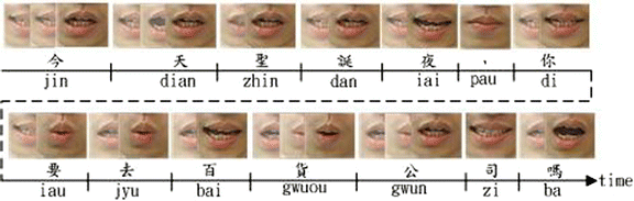
An example of image generation for viseme lip shapes arranged in time sequence
 ? (Today is Christmas Eve, will you go to the department store?)”, the phoneme recognition results (by HMM) in Mandarin are as follows: “/jin tian shien dan ie, ni iau qyu bai hwuo gwuen si ma/”; then pass to viseme classifier (by MCSVM). Finally, the lip shape images of classified viseme sequence are arranged into “/jin dian zhin dan iai, di iau jyu bai gwuou gwun zi ma/” as shown in Fig.
Vowel generally plays a major role, which are relatively stable during their pronunciation in lip shape determination. Oppositely, the lip shape varies rapidly with certain consonants when they are pronounced. Alpha blending is the process of combining a translucent foreground color with a background color, thereby producing a new blended color. Alpha blending uses the alpha values, or channel (bit mask) to represent the coverage of each pixel. The alpha value (between 0 ~ 1) is often said to represent ‘opacity’. This coverage information is used to control the compositing of colors (with RGB pixels). For properties of Mandarin speech, we use a different alpha blending algorithm for vowels and consonants, letting the visual quality be more fluid.
It is common to multiply the color by the alpha value if alpha channel is used in an image, because of saving the additional multiplications during blending; it is usually referred to as pre-multiplied alpha. For example, assume that the pixel color is expressed in RGBA tuples, and a pixel value of (0, 255, 0, 0.5) implies a pixel that is fully green and the alpha value is 0.5. Then rewrite it using pre-multiplied alpha, thus the tuples change into (0, 127.5, 0, 0.5).
For the existence of an alpha channel, it is easier to express compositing image. The RGB pixels from current image are mixed with the RGB pixels of previous image according to the formula as follow:
In order to let visual sense can be felt more smoothly about pictures conversion with alpha blending, we define some conditions as follows to detect viseme types for alpha value updating which is called dynamic alpha blending.
-
(i)
if previous and current is vowel, set alpha value = 1
-
(ii)
if previous is consonant and current is vowel, set alpha value = 0.7
-
(iii)
if previous is vowel and current is consonant, set alpha value = 0.3
4.2 Experimental Results
Table 6 shows the performance comparison of phoneme recognition using HMM. We evaluated conventional MFCCs to compare with the proposed ICA-Transformed MFCCs for the phoneme-error-rate (PER) and word-error-rate (WER) with clean speech, noisy speech (SNR = 10 dB) without/with the proposed speech enhancement. From this table, the proposed ICA-Transformed MFCCs method was better than conventional MFCCs method in three types of speech. For clean speech, the ICA-Transformed MFCCs could gain 4.4 % (15.6 % ~ 11.2 %) and 8.6 % (35.2 % ~ 24.8 %) accuracy rate improvements in PER and WER, respectively. For noisy speech with enhancement, comparing with clean speech, the accuracy rate is decreased in the range from 5.5 % (11.2 % ~ 16.7 %) to 14.8 % (15.6 % ~ 30.4 %) for PER and 5.6 % (24.8 % ~ 30.4 %) to 8.13 % (35.2 % ~ 43.33 %) for WER. This degradation was effectively lessened by passing the noisy input signal through our signal enhancement processing to generate enhanced input speech signal.
Vowel generally plays a major role, which are relatively stable during their pronunciation in lip shape determination. Table 7 shows the accuracy of viseme classification of vowel using MCSVM based on the proposed confusable phoneme-viseme mapping table (see Table 3). The average error rate is 19.22 % without mapping and 9.37 % with mapping. It is more helpful for lip shape image arrangement to presents more authenticity in visual quality.
Figure 9 describes the MOS result for our evaluation system with 10 users to score the visual quality rating and speech driven feeling that is real-time presentation. The result provides that interaction impression of speech-driven talking face system is satisfactory and simple animations receive positive evaluations from these questions. The score explains that our voice-driven system validation is 3.9 points on the average for each single vowel. And the isolated words with phoneme sequences scores is 3.7 on the average. Besides, the third question evaluated 3.6 scores is reflecting vivid in emtional interaction animation of the real-time system. The final question is to rate that whether we use dynamic alpha blending to synthesize human talking face is nature or not and the scores of it on average is 3.6.

Boxplot of the proposed system evaluation with MOS, where is median value and m is mean value
We also compared the averaged MOS test results with CrazyTalk [10] as shown in Fig. 10. The CrazyTalk is commercial software, and it should be fed with a recorded wave data to make the animations, it is an off-line speech driven system. Thus, the speech segmentation and the parameters of lip shape are easier processed than the real-time system in human talking face.

Result of MOS test of question sets
The result is proving that the real-time interaction impression of the voice-driven talking face system is satisfactory and simple animations receive positive evaluations from these questions. The score explains that our voice-driven system validation is 3.5 points on the average for each single vowel. And the isolated words with phoneme sequences scores is 3.18 on the average. Besides, the third question evaluated 3.2 scores is reflecting vivid in emotional expression animation of the real-time system. The final question is to estimate that whether we use alpha blending to synthesize human talking face is nature or not and the scores of it on average is 3.4.
5 Conclusion
In this paper, we describe our research using speech-driven talking face technology to work out defects in low bit-rate GSM communication which provides low computational complexity and smooth visual senses. A novel confusable phoneme-viseme mapping method using viseme histogram distance and viseme similarity measurement based on viseme visually ambiguous is proposed to simplify the mapping problem and promote viseme classification accuracy in this system. Acoustic feature of phoneme is extracted using ICA-based MFCCs and SNR-aware speech enhancement is used that can be clearly-distinct in spectrums and spectrum subtraction processing for canceling environmental noise during communication. HMM and MCSVM are combined as a recognition network approach for phoneme recognition and viseme classification
In experiments, comparing with clean speech, noise speech that was processed speech enhancement with ICA-based MFCCs, could gain 1.1 % (16.7 % to 15.6 %) and 4.8 % (30.4 % to 35.2 %) error rate improvements in PER and WER, respectively. For viseme classification, the error rate is decreased from 19.22 % to 9.37 %. Last, we evaluated a GSM communication environment for visual quality rating and speech driven feeling using mean opinion score (MOS). According to this, our method can effectively reduce the number of visemes and lip shape images by confusable phoneme-viseme mapping set and enable real-time operation. Besides, questionnaire, people feel more realizable and natural effects after appending real-time keyword recognition and interactive emotion expression. The system can be applied in interaction multimedia communication more widely.
The proposed system also can be implemented in remote interactive tutoring application such as distance learning, telemedicine and care system. If a user is sick and rest at home, there will a virtual agent with the camera, recording and display device in remote interactive tutoring application. Since the user is bed-sick, user can query the tutor and accept real-time tutoring by the virtual agent. Screen of the agent exploits voice driven talking face technology for display a real-time Q&A virtual image.
References
Bregler C, Covell M, Slaney M (1997) Video rewrite: Driving visual speech with audio. In Proc. ACM SIGGRAPH’97
Cambridge University Engineering Dept. HTK Toolkit 3.4. http://htk.eng.cam.ac.uk/
Chen T (2001) Audiovisual speech processing: Lip reading and lip synchronization. IEEE Signal Process Mag 18(1):9–21
Chen T, Rao RR (1998) Audio-visual integration in multimodal communication. Processing of the IEEE 86(5):837–852
Choi K, Luo Y, Hwang J-N (2001) Hidden Markov model inversion for audio-to-visual conversion in an MPEG-4 facial animation system. The Journal of VLSI Signal Processing 29(1–2):51–61
Cohen MM, Massaro DW (1993) Modeling coarticulation in synthetic visual speech. In: Magnenat-Thalmann M, Thalmann D (eds) Models and techniques in computer animation. Springer, Tokyo, pp 139–156
Cosatto E, Graf HP (1998) Sample-based synthesis of photo-realistic talking heads. in Proc. IEEE Computer Animation, pp. 103–110
Cosatto E, Graf HP (2000) Photo-realistic talking heads from image samples. IEEE Trans Multimedia 2:152–163
Cosatto E, Ostermann J, Graf HP, Schroeter J (2003) Lifelike talking faces for interactive services. Proc IEEE 91(9):1406–1428
CrazyTalk, V 2.0 Lip-Sync, 2010. Http://www.reallusion.com/Crazytalk/.
Curinga S, Lavagetto F, Vignoli F (1996) Lip movements synthesis using time delay neural networks. in Proc. EUSIPCO 96—Systems and Computers, pp. 36–46
Ephraim Y, Trees HLV (1995) A signal subspace approach for speech enhancement. IEEE Transactions on Speech and Audio Processing 3(4):251–266
Ezzat T, Geiger G, Poggio T (2002) Trainable videorealistic speech animation. Proc ACM SIGGRAPH’02 21(3):388–397
Imperl B, Horvat B (1999) The clustering algorithm for the definition of multilingual set of context dependent speech models. In Proceedings of the European Conference of Speech Communication and Technology, pp. 887–890
Koster BE, Rodman RD, Bitzer D (1994) Automated lip-sync: Direct translation of speech-sound to mouth-shape. in Proc. 28th Annu. Asilomar Conf. Signals, pp. 583–586
Lee S, Yook D (2002) Audio-to-visual conversion using hidden Markov models. In Proceedings of the 7th Pacific Rim International Conference on Artificial Intelligence, Springer-Verlag, pp. 563–570
Lucey P, Martin T, Sridharan S (2004) Confusability of phonemes grouped according to their Viseme classes in noisy environments. Presented at tenth Australian international conference on speech science & technology. Macquarie University, Sydney
Mcallister DV, Rodman RD, Bitzer DL, Freeman AS (1997) Lip synchronization for Animation. Proc. SIGGRAPH 97, Los Angeles, CA, pp. 225–228
Morishima S (1998) Real-time talking head driven by voice and its application to communication and entertainment. in Proc. AVSP 98, pp. 195–200
Ostermann J, Weissenfeld A (2004) Talking faces-technologies and applications. In Proc of ICPR’04 3:826–833
Park J, Ko H (2008) Real-time continuous phoneme recognition system using class-dependent tied-mixture HMM with HBT structure for speech-driven lip-sync. IEEE Trans Multimedia 10(7):1299–1306
Parke F, Waters K (1996) Computer facial animation
Tamura M, Masuko T, Kobayashi T, Tokuday K (1998) Visual speech synthesis based on parameter generation from HMM: Speech driven and text-and-speech driven approaches. in Proc. Audio-Visual Speech Processing (AVSP 98), pp. 221–226
Theobald B, Bangham A, Matthews I, Cawley G (2004) Near-videorealistic synthetic talking faces: Implementation and evaluation. Speech Communication 44:127–140
Theobald BJ, Wilkinson N (2007) A real-time speech-driven talking head using active appearance models. AVSP 2007, international conference on auditory-visual speech processing 2007. Kasteel Groenendael, Hilvarenbeek
Turunen E (2001) Survey of theory and applications of Lukasiewicz-Pavelka fuzzy logic. Lectures on Soft Computing and Fuzzy Logic. Advances in Soft Computing, pp. 313–337
Wang HC (1997) MAT—A project to collect Mandarin speech data through telephone networks. Computational Linguistics and Chinese Language Processing, Computational Linguistics Society of R.O.C., vol.2, no. 1, pp. 73–90.
Wang J-C, Lee H-P, Wang J-F, Lin C-B (2008) Robust environmental sound recognition for home automation. IEEE Transaction on Automation Science and Engineering 5(1):25–31
Wang J-C, Lee H-P, Wang J-F, Yang C-H (2007) Critical band subspace-based speech enhancement using SNR and auditory masking aware technique. IEICE Trans Inf Syst E90-D(7):1055–1062
Xie L, Liu Z (2007) Realistic mouth-synching for speech-driven talking face using articulatory modeling. IEEE Trans Multimedia 9(3):500–510
Yamamoto E, Nakamura S, Shikano K (1998) Lip movement synthesis from speech based on Hidden Markov models. Speech Communication 26(1–2):105–115
Ye J, Yao H, Jiang F (2004) Based on HMM and SVM multilayer architecture classifier for chinese sign language recognition with large vocabulary. Proc. Third Int’l Conf. Image and Graphics (ICIG’04), 377–380
Zgank A, Imperl B, Johansen F (2001) Crosslingual speech recognition with multilingual acoustic models based on agglomerative and tree-based triphone clustering. In Proceedings of the European Conference of Speech Communication and Technology, pp. 2725–2728
Zhong D, Defée I (2007) Performance of similarity measures based on histograms of local image feature vectors. J Patt Recog Lett 28(15)
Acknowledgments
This research is partially support by National Cheng Kung University and NSC Research Fund.
Author information
Authors and Affiliations
Corresponding author
Rights and permissions
About this article
Cite this article
Shih, PY., Paul, A., Wang, JF. et al. Speech-driven talking face using embedded confusable system for real time mobile multimedia. Multimed Tools Appl 73, 417–437 (2014). https://doi.org/10.1007/s11042-013-1609-3
Published:
Issue Date:
DOI: https://doi.org/10.1007/s11042-013-1609-3