
Abstract
We consider a variant of the multi-armed bandit model, which we call scratch games, where the sequences of rewards are finite and drawn in advance with unknown starting dates. This new problem is motivated by online advertising applications where the number of ad displays is fixed according to a contract between the advertiser and the publisher, and where a new ad may appear at any time. The drawn-in-advance assumption is natural for the adversarial approach where an oblivious adversary is supposed to choose the reward sequences in advance. For the stochastic setting, it is functionally equivalent to an urn where draws are performed without replacement. The non-replacement assumption is suited to the sequential design of non-reproducible experiments, which is often the case in real world. By adapting the standard multi-armed bandit algorithms to take advantage of this setting, we propose three new algorithms: the first one is designed for adversarial rewards; the second one assumes a stochastic urn model; and the last one is based on a Bayesian approach. For the adversarial and stochastic approaches, we provide upper bounds of the regret which compare favorably with the ones of Exp3 and UCB1. We also confirm experimentally that these algorithms compare favorably with Exp3, UCB1 and Thompson Sampling by simulation with synthetic models and ad-serving data.
1 Introduction
In its most basic formulation, the multi-armed bandit problem can be stated as follows: there are K arms, each having an unknown, and infinite sequence of bounded rewards. At each step, a player chooses an arm and receives a reward issued from the corresponding sequence of rewards. The player needs to explore the arms to find profitable actions, but on other hand the player would like to exploit as soon as possible the best arm identified. Which policy should the player adopt in order to minimize the regret against the best arm?
The stochastic formulation of this problem assumes that each arm delivers rewards that are independently drawn from an unknown distribution. Efficient solutions based on optimism in the face of uncertainty have been proposed for this setting (Lai and Robbins 1985; Agrawal 1995). They compute an upper confidence index for each arm and choose the arm with the highest index. In this case, it can be shown that the regret, the cumulative difference between the optimal reward and the expectation of reward, is bounded by a logarithmic function of time, which is the best possible. Subsequent work introduced simpler policies, proven to achieve logarithmic bound uniformly over time (Auer et al. 2002a). Recently, different variants of these policies have been proposed, to take into account the observed variance (Audibert et al. 2009), based on Kullback-Leibler divergence (Garivier and Cappé 2011), the tree structure of arms (Kocsis and Szeoesvàri 2006; Bubeck et al. 2008), or the dependence between arms (Pandey et al. 2007).
Another approach to solve the multi-armed bandit problem is to use a randomized algorithm. The Thompson Sampling algorithm, one of the oldest multi-armed bandit algorithm (Thompson 1933), is based on a Bayesian approach. At each step an arm is drawn according to its probability of being optimal. The observation of the reward updates this probability. Recent papers have shown its accuracy on real problems (Chapelle and Li 2011), and that it achieves logarithmic expected regret (Agrawal and Goyal 2012), and that it is asymptotically optimal (Kaufman et al. 2012b).
There are however several applications, including online advertising, where the rewards are far from being stationary random sequences. A solution to cope with non-stationarity is to drop the stochastic reward assumption and assume the reward sequences to be chosen by an adversary. Even with this adversarial formulation of the multi-armed bandit problem, a randomized strategy like Exp3 provides the guarantee of a minimal regret (Auer et al. 2002b; Cesa-Bianchi and Lugosi 2006).
Another usual assumption which does not fit well the reality of online advertising is the unlimited access to actions. Indeed, an ad server must control the ad displays in order to respect the advertiser’s budgets, or specific requirements like “this ads has to be displayed only on Saturday”. To model the limited access to actions, sleeping bandits have been proposed (Kleinberg and Niculescu-Mizil Sharma 2008). At each time step, a set of available actions is drawn according to an unknown probability distribution or selected by an adversary. The player then observes the set, and plays an available action. This setting was later completed to take into account adversarial rewards (Kanade et al. 2009). Another way to model the limited access to actions is to consider that each arm has a finite lifetime. In this mortal bandits setting, each appearing or disappearing arm changes the set of available actions. Several algorithms were proposed and analyzed by Chakrabarti et al. (2008) for mortal bandits under stochastic reward assumptions.
In this paper, we propose a variant of mortal and sleeping bandits, which we call scratch games, where the sequences of rewards are finite and drawn in advance with known lengths, and with unknown starting dates. We assume the sequences lengths to be known in advance: indeed, the maximum display counts are usually fixed in advance by a contract between the advertiser and the publisher. This knowledge makes our setting different from sleeping bandits where the sequences of reward are infinite. The ad serving optimization is a continuous process which has to cope with appearing and disappearing ads along the way. During a long period of time, it is not possible to know in advance the number of ads that the ad server has to display, since it depends of new contracts. To fit this application constraints, for the scratch games setting, the starting dates of new scratch games and the maximum number of scratch games are unknown to the player. This point differs from mortal bandits.
We consider both an adversarial reward setting where the sequences are determined by an oblivious adversary and a stochastic setting where each sequence is assumed to be drawn without replacement from a finite urn. These two settings extends and complete the work of Chakrabarti et al. (2008). The non-replacement assumption is better suited to the sequential design of non-reproducible experiments. This is the case for telemarketing where each targeted client is only reachable once for each campaign. This is also the case for targeted online advertising when the number of display of a banner to an individual is limited. This limit, called capping, leads to an urn model (formally when the capping is set to one).
In Sect. 2, we give a formal definition of scratch games. Then, we will propose three algorithms, based on different assumptions to exploit and explore finite sequences of rewards with unknown starting dates:
-
the first one (in Sect. 3), E3FAS, is a randomized algorithm based on a deterministic assumption: an adversary has chosen the sequences of rewards,
-
the second one (in Sect. 4), UCBWR, is a deterministic algorithm based on a stochastic assumption: the sequences of rewards are drawn without replacement according to unknown distributions,
-
the last one (in Sect. 5), TSWR, is a randomized algorithm based on a Bayesian assumption: the mean reward of each scratch games is distributed according to a beta-binomial law.
For the first two, we will provide regret bounds for scratch games, which compare favorably to the UCB1 and Exp3 bounds. In Sect. 6, we will test these policies on synthetic problems to study their behavior with respect to different factors coming from application constraints. We will complete these tests with a realistic ad serving simulation.
2 Problem setup: scratch games
We consider a set of K scratch games. Each game i has a finite number of tickets N i including M i winning tickets, and a starting date t i . Let x i,j be the reward of the j-th ticket for game i. We assume that the reward of each ticket is bounded: 0≤x i,j ≤1. A winning ticket is defined as a ticket which has a reward greater than zero.
The number of tickets N i of current games are known to the player.
The number of winning tickets M i , the starting dates t i of new scratch games, the total number of scratch games K, and the sequence of reward x i,j of each game are unknown to the player.
At each time step t, the player chooses a scratch game i in the set of current scratch games [K t ], and receive the reward \(x_{i,n_{i}(t)}\), where n i (t) is the number of scratched tickets at time t of the game i.
In the following to simplify the notations, we will use i t to denote the game played at time t, and x i (t) for \(x_{i,n_{i}(t)}\). When n i (t)=N i , all the tickets have been scratched and x i (t)=0. At time t, a policy π chosen in the set of possible policies Π, allows the player to choose the next scratch game i t . A policy can be static if the sequence of chosen games is fixed at the beginning, or dynamic if the choice of the next game is determined by the sequence of past rewards \(x_{i_{1}} (1), x_{i_{2}} (2),\ldots, x_{i_{t-1}} (t-1)\). A policy can be randomized, if the next game is drawn according to a probability distribution, or deterministic if at time t only one game can be chosen. By applying a policy π, at time T a sequence of choices is obtained (i 1,i 2,…,i T ). At time T, the gain of the policy π is:
The scratch game problem is different from the multi-armed bandit problem. Indeed, in the multi-armed bandit setting, to maximize his gain the player has to find the best arm as soon as possible, and then exploit it. In the scratch game setting, the number of tickets is finite. When the player has found the best game, he knows that this game will expire at a given date. The player needs to re-explore before the best game finishes in order to find the next best game. Moreover, a new best game may appear. The usual tradeoff between exploration and exploitation has to be revisited. In the next sections, we will detail respectively adversarial, stochastic, and stochastic Bayesian declinations for the scratch games of the well known algorithms Exp3 (Auer et al. 2002b), UCB1 (Auer et al. 2002a), and TS (Thompson 1933) used for the multi-armed bandits.
3 Adversarial bandit algorithms for scratch games
3.1 Introduction
In this section, we will assume that the number of winning tickets M i , the sequence of rewards x i (1),x i (2),…,x i (N i ), and the starting date t i of each scratch game are chosen by an adversary. The number of tickets N i , and the starting date t i of current scratch games i are known by the player. We assume that the adversary is oblivious. His policy is assumed to be static: the sequences of rewards are chosen at t=0 and never change during the game. At time t, the optimal static policy chooses from the current scratch games, the one with the best next ticket. Then, at time T the optimal static policy has a gain of:
where K t is the number of current scratch games at time t, and [K t ] denotes the set of current scratch games at time t. We would like to find an efficient policy to optimize the rewards knowing the number of tickets T a player wishes to play. We extend the notion of weak regret of a policy π chosen in the set of policies Π, defined by Auer et al. (2002b) as the regret against the best single arms, to the regret against the optimal static policy:
In order to simplify notation, we will use G T for G T (π) and R T for R T (π). We would like to find policies which give us guaranties for all the sequences of rewards chosen by the adversary. Following Auer et al. (2002b), we will use randomized policies. To evaluate the efficiency of these policies, we will take the gain expectation with respect to the probability distribution of i t knowing the past choices i 1,i 2,…,i t−1. The expected weak regret is defined by:
3.2 E3FAS
Exp3 (Exponential weight algorithm for Exploration and Exploitation) is a powerful and popular algorithm for adversarial bandits (Auer et al. 2002b). The Achilles heel of this algorithm is its sensitivity to the exploration parameter γ: a value too low or too high for this parameter leads to a bad trade-off between exploitation and exploration. The intuition used to adapt Exp3 to scratch games is the following: when a new game starts the exploration term γ has to increase in order to explore it, and when a game ends, the number of games decreases and the exploration term γ has to decrease.
The proposed algorithm, E3FAS (Exponential weight algorithm for Exploration and Exploitation of Finite and Asynchronous Sequences), consists in reevaluating the exploration term γ m each time a game starts or ends (see Algorithm 1). As the weights store the estimated mean reward of each game, each time T m the parameter γ m is recalculated, we keep the value of the weights. For reasons of digital precision, we reset the weights in a way that their sum is equal to the number of games and that the probability to draw a game does not change (see Algorithm 1). We initialize the weights of new scratch games at the mean value of existing weights. Then, when a new scratch games i starts, it has a probability to be drawn of:

E3FAS policy is an adaptation of Exp3 policy for scratch games
Let T m be the time when a game starts or ends, T m+1 be the time when another game starts or ends, K m be the number of games during the time period [T m ,T m+1[, \(\varDelta_{m}=G_{T_{m+1}}-G_{T_{m}}\) be the gain between times T m and T m+1 and \(\varDelta ^{*}_{m}=G^{*}_{T_{m+1}}-G^{*}_{T_{m}}\) be the optimal gain between times T m and T m+1. We first give an upper bound for the expected regret obtained by E3FAS for a given period and a given γ m .
Theorem 1
fig9 For all K m >0, if E3FAS policy runs from time T m to time T m+1, with 0<γ m ≤1, then we have:
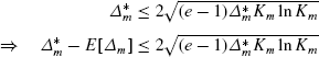
If the optimal gain \(\varDelta^{*}_{m}\) is known, we can use this bound to evaluate the value of γ m each time a game ends or starts. We use \(\gamma_{m}^{*}\) to denote the value of the parameter γ m which optimizes the upper bound given by Theorem 1.
Corollary 1.1
For all K m >0, if E3FAS policy runs from time T m to time T m+1, with 0<γ m ≤1, then we have:
Corollary 1.2
If E3FAS policy runs from the time t=0 to the time t=T, and K m >0 for the L time periods [T m ,T m+1[, we have:

The proofs of Theorem 1 and Corollaries 1.1 and 1.2 can be found in the Appendix. The obtained bound (the first inequality) is less or equal to the one of Exp3 for the scratch games (the second inequality). Notice that these upper bounds of the weak regret for scratch games are theoretical: Exp3 requires the knowledge of \(G_{T}^{*}\) and K, while E3FAS requires the knowledge of a the number of time periods L, the numbers of scratch games K m , and the values of \(\varDelta_{m}^{*}\).
In practice, at time T m to evaluate the value of the parameter \(\gamma^{*}_{m}\) using Corollary 1.1, we need to guess the value of \(\varDelta^{*}_{m}\). First, notice that the length of a given time period [T m ,T m+1[ is unknown to the player. At any time a new game may appear, and the end of a current game depends on a randomized algorithm and on the sequences of reward, which are unknown to the player. The only knowledge that has the player is that T m+1 cannot be higher than the minimum of T and the number of remaining tickets of the current games minus the number of current games, then:
Then, we bound the value of \(\varDelta_{m}^{*}\) at time T m by:
In real application, the order of magnitude of the mean reward of all games μ is usually known. For example, μ≈1/1000 for the click-through-rate on banners, μ≈1/100 for emailing campaigns, and μ≈5/100 for telemarketing. In these cases, it is reasonable to assume that \(G^{*}_{T} \approx\mu T \ll T\). If this prior knowledge is not available, it is possible to use T to bound \(G_{T}^{*}\).
4 Stochastic bandit algorithms for scratch games
4.1 Introduction
In this section, we assume that for each game i, the rewards of each ticket have been drawn independently and identically according to an unknown probability law, thus forming an urn model. The number of scratch games K, and the starting dates of new games are unknown and still chosen by the environment. μ i is the mean reward of the game i, and μ is the mean reward of all games. Here, x i (t) is a random variable giving the reward of the n i (t)-th ticket for the game i. Following (Agrawal 1995; Lai and Robbins 1985; Auer et al. 2002a), we propose to evaluate an index for each game i to choose the best game at each time step t. The expected gain of this deterministic policy is:
Where G t (i) is the cumulated reward of game i. The expectation is taken over the sequences of draws \(x_{i_{1}} (1), x_{i_{2}} (2),\ldots, x_{i_{t}} (t)\) according to the probability law of each game i. Knowing the number of tickets N i , the starting date t i of each current scratch game i, we would like to find an efficient policy in order to optimize uniformly the expected gain E[G t (π)] over all the sequences of draws.
The optimal policy exploits the difference between the mean reward μ i of each game i and the estimated reward \(\hat{\mu}_{i}(t)\) to choose the best remaining game. However, to provide bounds on the regret, we evaluate it against the optimal static policy. It consists in sorting current games i by decreasing mean rewards, and then playing each game until its number of remaining tickets is zero or until a new game with an highest mean reward appears. We denote \(i_{t}^{*}\) the game chosen by the optimal static policy at time t. We define Δ i (t) as the difference between the mean reward of the game i chosen by a policy and the mean reward of the game chosen by the optimal static policy:
Notice that the game chosen by the optimal static policy does not depend on the sequence of scratched tickets. It depends only on the starting date t i , the number of tickets N i and on the mean reward μ i . Δ i (t) is deterministic. This property will be useful below to provide bounds on E[n i (t)] in order to compare algorithms. Finally, we define the weak regret R as:
4.2 UCBWR
UCB1 policy (Auer et al. 2002a) is based on the Chernoff-Hoeffding inequality. Its use supposes that the rewards are drawn independently. This assumption does not hold for drawing without replacement. In this case, the Serfling inequality (Serfling 1974) can be used. Let x 1,…,x n be a sample drawn without replacement from a finite list of values X 1,…,X N between 0 and 1 with a mean value of μ, then for all ϵ>0:
We propose to use the Serfling inequality rather than Chernoff-Hoeffding inequality to build an upper confidence bound for scratch game (Féraud and Urvoy 2012). Let B i (t) be the index of game i at time t:
where t i >t is the starting date of the scratch game i. It allows us to evaluate the upper confidence bound of a new game. As in UCB1, the index B i (t) is used to sort each game at time t and then to play the game with the highest index (see Algorithm 2). We call this policy UCBWR for Upper Confidence Bounds for drawing Without Replacement. In the following, we will call the sampling rate the ratio (n i (t)−1)/N i .

UCBWR policy is an adaptation of UCB1 policy for the scratch games
With UCBWR policy, the mean reward is balanced with a confidence interval weighted by one minus the sampling rate of the game. Then, when the number of plays n i (t) of the scratch game i increases, the confidence interval term decreases faster than with UCB1 policy. The exploration term tends to zero when the sampling rate tends to 1. The decrease of the exploration term is justified by the fact that the potential reward decreases as the sampling rate increases. Notice that if all games have the same sampling rates, the rankings provided by UCB1 and UCBWR are the same. The difference between rankings provided by UCBWR and UCB1 increases as the dispersion of sampling rates increases. We can expect different performances, when the initial numbers of tickets N i are different. In this case, scratching a ticket from a game with a low number of tickets has more impact on its upper bound than from a game with a high number of tickets.
Theorem 2
For all K>1, if policy UCBWR is run on K scratch games j of size N j , with a unknown starting date t j , then for any suboptimal scratch game i with N i >0, t>t i we have:
The bound obtained by UCBWR policy is less or equal than the one obtained applying UCB1 policy (the right term of the inequality of Theorem 2) to scratch game:
-
equal at the initialization when the expected sampling rate is zero,
-
and lower when the expected sampling rate increases.
Corollary 2.1
For all K>1, if policy UCBWR is run on K scratch games j of size N j , with a unknown starting date t j , then at time t the weak regret is bounded by:
The proofs of Theorem 2 and Corollary 2.1 can be found in the Appendix.
5 Bayesian bandit algorithms for scratch games
5.1 Introduction
In this section, we assume the rewards of each ticket to be binary values (x i (t)∈{0,1}) which have been drawn independently and identically according to an unknown probability law. Each scratch games is a set of N i tickets, with M i winning tickets. We recall that μ i denotes the mean reward of game i, such that M i =N i μ i . Under these assumptions, corresponding to the urn model, the probability to observe m i winning tickets is computed with the hypergeometric law:
Notice that the parameter μ i can take N+1 discrete values of form j/N i , with j∈{0,1,…,N i }. Assuming that no value is more likely than any other, we choose P(μ i |n i =0,N i )=1/(N i +1). Using the Bayes rule, we can compute the posterior distribution of the mean reward μ i , with m i ≤Nμ i ≤N i −n i (see Briggs and Zaretzki 2009):

where β(a,b) denotes the beta function. The obtained posterior distribution is the beta-binomial distribution.
5.2 Thompson sampling without replacement
The Thompson sampling algorithm repeatedly draws μ i (t) according to its posterior distribution and chooses the game corresponding to the maximum mean reward. The observation of reward updates the posterior distribution (see Algorithm 3). When the number of draws of a game is low, the posterior distribution has a large variance, which promotes the exploration of this game. When a game has been chosen a lot of times, its posterior distribution is sharp, to promote exploitation of game i with high value of μ i .

TSWR policy is an adaptation of Thompson Sampling for the scratch games
The Thompson sampling algorithm is a generic algorithm which can be applied with various priors. In the case of a Bernoulli distribution of rewards, recent papers have shown that it achieves logarithmic expected regret (Agrawal and Goyal 2012) and that it is asymptotically optimal (Kaufman et al. 2012b). We propose to use the Thompson sampling algorithm to the scratch games using a beta-binomial law to model the parameters likelihood rather than the beta law used for the multi-armed bandits (Chapelle and Li 2011).
To speed up the convergence of the algorithm, we can use the value of the mean reward of all games μ, which is often known in real application, for initializing the values of m i , n i , and μ i of each game i: we choose the initial value μ i =μ for having a prior in the order of magnitude of its true value, and we choose m i =1, and n i =1/μ i in order to begin with a large variance around this initial prior. For example, the click-through rate on a web-portal is approximatively of 1/1000. In this case, we will use to initialize the game i: μ i =1/1000, m i =1, n i =1000. When μ is unknown, μ i can be initialized to any value lesser than 1, with m i =0 and n i =0.
We do not provide bounds of the regret for Thomson Sampling Without Replacement, and to the best of our knowledge, it is an open problem.
6 Experimental results
6.1 Experimental setup
We have proposed three algorithms taking into account that the sequences of rewards are finite, and drawn in advance with unknown starting dates. These three algorithms will be compared to Exp3 (Auer et al. 2002b), UCB1 (Auer et al. 2002a), and TS for the Thompson sampling for the Bernoulli bandit (Chapelle and Li 2011). For all policies when the number of tickets of a scratch game reaches zero, the scratch game is suppressed from the list of games. In the case of Exp3 to evaluate the value of γ ∗, we assume that the number of scratch games K is known and we use the bound of the expected gain coming from the analysis of weak regret for infinite sequences of rewards proposed by Auer et al. (2002b):
We have supposed that \(G_{T}^{*}\) is known, and we have used it for Exp3, E3FAS, TS, and TSWR. In order to compare significantly the algorithms, we have plotted the estimated weak regret on one hundred trials versus the number of scratched tickets, t:
For each scratch game, each trial corresponds to a different sequence of binary rewards, drawn in an urn, where the number of tickets and the number of winning tickets are the parameters. The optimal policy used to evaluate the regret is the optimal static policy for the stochastic scratch games (see Sect. 4.1). The error bar of each point of curves, corresponding to the confidence interval at 95 %, is plotted. In order to sum up, we have evaluated the mean of the estimated weak regret during the time period [1,N]:
where N is the total number of tickets, known at the end of the simulation.
6.2 Synthetic problem
In this section, we would like to analyze the behavior of algorithms with respect to different factors coming from our application constraints:
-
1.
Due to the budget constraints, the scratch games have finite sequences of rewards.
-
2.
Due to the continuous optimization, the scratch games have different and unknown starting dates.
-
3.
Due to the competition between ads on a same target (cookies, profiles …), to the relevance of the ad with page content, which can change, and to unknown external factors, the mean reward of a scratch game can change over time.
We have chosen a Pareto distribution to draw the number of tickets of 100 scratch games, with parameters x m =200 and k=1. This choice is driven by the concern to be as close as possible to our application: a lot of small sequences and a small number of very large sequences. The number of winning tickets of each scratch game is drawn according to a Bernoulli distribution, with parameter p i drawn from a uniform distribution between 0 and 0.25. 210314 tickets including 33688 winning tickets spread over 100 scratch games are drawn. For each trial and for each scratch game i, a sequence of rewards is drawn according to the urn model parametrized by the number of winning tickets m i and the number of tickets n i .
To investigate the behavior of algorithms for finite sequences, we have plotted the number of remaining games versus the number of scratched tickets (see Fig. 1). The optimal static policy plays the scratch games in decreasing order of mean reward. we observe that UCBWR, and TS tend to keep games longer than the optimal static policy. The Serfling upper bound decreases at the same rate as the square root of the sampling rate. Then, UCBWR tends to explore more the games with an high number of tickets, where the decreasing of the sampling rate is low and where the potential remaining reward is high. The Thompson sampling algorithm works in a different way. It spends tickets to estimate the distribution of the mean rewards of each game. When these estimations are sharp, it tends to draw a game with an high mean reward, which has a lot of tickets. The use of the hypergeomtric law in place of Bernoulli law enhances the probability of drawing small scratch games. TSWR plays first the small games with high mean rewards. Exp3 and E3FAS are more conservative and they switch all the time between games. As a consequence, the games with a small number of tickets finish earlier.

The number of remaining games versus the number of scratched tickets
When the numbers of tickets are drawn according to a Pareto distribution, there are a few number of games with a lot of tickets. In this case, UCB1 spends too much time to explore the small games and as expected by our theoretical analysis, UCBWR outperforms UCB1 (see Fig. 2 and Table 1). The values of parameter γ evaluated for E3FAS take into account that the sequences of rewards are finite. The initial value is the same for Exp3 and E3FAS, and then for E3FAS γ is decreased progressively each time a game is ended, until it reaches zero. In the case of scratch games, the re-estimations of the value of the parameter γ lead to a better trade-off between exploration and exploitation. This experimental result confirms our theoretical analysis (see Fig. 2 and Table 1): E3FAS outperforms Exp3 on the second part of the curve, when the number of ended games is high. As expected, the Thompson sampling without replacement (TSWR) based on a beta-binomial prior slightly outperforms the Thompson Sampling (TS) based on a beta prior (Table 1). On the first part of the curves, TS outperforms TSWR: the number of tickets is high and the distribution of rewards is close to a Bernoulli law. However, on the second part of the curves, the number of tickets is low, and the effect of the draws without replacements favors TSWR. On this problem, as expected from the analysis of the algorithms, it seems possible to take advantage of the scratch games problem for the different settings: adversarial (E3FAS vs Exp3), stochastic (UCBWR vs UCB1) or Bayesian (TSWR versus TS). The Thompson sampling algorithms are the best: they converge faster, and they are the closest to the optimal static policy.

The weak regret versus the number of scratched tickets for a Pareto distribution
In the second synthetic problem, 50 % of the games begin after that 100000 tickets have been scratched. For UCB1 and UCBWR, the starting dates are used in the evaluation of the indexes, for Exp3, and E3FAS, the weights of new scratch games are initialized to the mean value of weights and for TS and TSWR new games are initialized to the prior. The Thompson sampling algorithms are still the best (see Fig. 3 and Table 1). We observe that in this case UCBWR outperforms Exp3 and E3FAS. UCBWR finds more quickly the new best games, thanks to its exploration factor which advantages the exploration of new games (high confidence interval due to their low sampling rate).

The weak regret versus the number of scratched tickets for asynchronous start of games
In the last synthetic problem, we test the behavior of algorithms on non-stationary distributions using a threshold function:
-
for games with even index, during the time period [0,N/2] the probability of reward is multiplied by two, and during the time period [N/2,N] the probability of reward is divided by two.
-
otherwise, during the time period [0,N/2] the probability of reward is divided by two, and during the time period [N/2,N] the probability of reward is multiplied by two.
We observe that the optimal static policy for stochastic scratch games is not well suited, when the distributions of rewards change during time (Fig. 4). The number of winning tickets of each scratch games does not change, but during the two time periods some games can provide more or less winning tickets than expected. That is why dynamic policies can sometimes have a negative regret. As expected, the adversarial multi-armed bandits are well suited for non-stationary distributions of rewards (see Fig. 4 and Table 1). TSWR algorithm is based on a prior which does not hold here. Even if the probability of rewards is multiplied by two for several scratch games during the first time period, the number of winning tickets does not change. When all the winning tickets have been scratched this probability vanishes. Then, the prior on the corresponding parameter μ i suddenly becomes false, and as TSWR tends to play first the small games, its performance collapses during the first time period. For TS, the same phenomena appends when at time N/2, the probability of rewards of scratch games with uneven index are multiplied by 2. The Thompson Sampling algorithms are the worst in this case. Surprisingly, UCBWR performs very well on this problem. On the first period, as all algorithms, it plays more even scratch games which have their probabilities of rewards multiplied by two. However, thanks to the decreasing of its exploration factor, it does not scratch all the tickets of these games. For the introduced non-stationarity it is useful because most of the winning tickets of even games have been scratched before the end of this time period. We can suspect that on more complex non-stationary sequences, the performances of UCBWR would collapse.

The weak regret versus the number of scratched tickets when the distributions of rewards depends on a threshold function of time
In these illustrative synthetic problems, we observe that if its prior holds, the Thompson Sampling algorithm Without Replacement is the best, and for the tested non-stationary distributions of rewards it is one of the worst. UCBWR is an efficient and robust algorithm which obtains good performances on the three synthetic problems. E3FAS also exhibits good performances, and it provides more guarantees on non stationary data. Finally, we observe that algorithms designed for scratch games outperform those designed for multi-armed bandits: for adversarial approach E3FAS outperforms Exp3, for stochastic approach UCBWR outperforms UCB1, and for Bayesian approach TSWR outperforms TS. In the next section we will test the same algorithms on complex real data.
6.3 Test on ad serving data
In the pay-per-click model, the ad server displays different ads on different contexts (profiles × web pages) in order to maximize the click-through rate. To evaluate the impact of E3FAS, Exp3, UCBWR, UCB1, TS and TSWR on the ad server optimization, we have simulated it.
We have collected for a given web page the sequences of the tuples corresponding to the ad displays and clicks per minute for 309 ads, during seven days, for a sample of 1/10 of the users. 309 asynchronous sequences are obtained. It corresponds to a total of 10730000 displays and 84445 clicks. In this simulation we consider only one instance of the distributions of clicks on one page. However, notice that the size of these sequences is two order of magnitudes higher than the ones of the synthetic problems. Moreover, for obtaining realistic conditions for the simulation, we have chosen a web page currently used for the pay-per-click and a time period of one week, where the variability of the sequences of clicks is high (see Fig. 6). We observe that as in the synthetic problem (see Sect. 6.2), the distribution of the number of displays is close to a Pareto distribution (see Fig. 5a). We have plotted the starting dates of ads in decreasing order: during the simulation approximately 25 % of new ads will arrive (see Fig. 5b).

On the left (a), the distribution of the number of displays. On the right (b), the starting dates of ads in decreasing order
Each ad is considered as a scratch game, with a finite number of tickets corresponding to the number of displays, including a finite number of winning tickets corresponding to the clicks, and with a sequence of rewards corresponding to sequences of ad displays and clicks. When a scratch game is selected by a policy, the reward is read from its sequence of rewards. In the simulation, we consider that the observed displays of each ad represent their total inventories on all web pages. The goal of the optimization is then to increase the number of displays of the ads with a high click-through rate and to decrease the number of displays of the others.
On these real sequences of clicks, the distributions of rewards are bursty, seem to have a lot of states, and they cannot have been generated independently and identically (see Fig. 6). The results of this simulation confirm those obtained on the synthetic problem (see Fig. 7 and Table 1): we can take advantage of the scratch games setting to improve the performances of standard multi-armed bandit algorithms. On these complex distributions of rewards (see Fig. 6), as expected the adversarial multi-armed bandits outperform the others. The Thompson Sampling algorithms converge fast to the posterior distribution of the parameter (here the mean number of clicks), but when the distribution of data changes quickly, they cannot adapt. The result obtained by the policy TS is similar to the one obtained by a random policy (RAND) and TSWR slightly outperforms the random policy. The regret curves of the policies UCB1 and UCBWR are tight, and UCBWR outperforms UCB1.

Two sequences of CTR by time step of one minute generated by two ads on a given web page. There is a lot of bursts, and these distributions cannot be generated independently and identically by an hypergeometric or a Bernoulli law

The weak regret of tested policies. On these real data, the adversarial multi-armed bandits outperforms the others. Exp3 and E3FAS are the best and TSWR is the worst
Finally, we have plotted the gain of the policies (here the number of clicks) to evaluate the potential increase of incomes of this ad serving optimization (see Fig. 8). When 20 % of ads have been sent, the number of clicks generated by the adversarial multi-armed bandits is approximately two times better than a random ad serving, and 1.5 times better than the one generated by the stochastic multi-armed bandit policy.

The number of clicks versus the number of displays. when 20 % of ads have been displayed. The number of clicks generated using E3FAS or Exp3 is 1.5 time higher than the one of UCB1 or UCBWR
In this experiment, we have considered a simple context: the optimization of a single page for all profiles of cookies during one week. The optimization over a long period of time of many pages for several profiles of cookies will generate many scratch games. As the number of scratch games K increases, the difference between the regret bounds of Exp3 and the one of E3FAS increases (see Corollary 1.2). We can expect more significant differences of gains between Exp3 and E3FAS. Notice that for an optimization over a long period of time, such as several months, to tune the exploration factor of E3FAS, we have to consider a sliding time horizon T as a parameter of the optimization, that we have to tune. UCBWR does not suffer from this drawback.
7 Conclusion
We have proposed a new problem to take into account finite sequences of rewards drawn in advance with unknown starting dates: the scratch games. This problem corresponds to applications where the budget is limited, and where an action cannot be repeated identically, which is often the case in real world. We have proposed three new versions of well known algorithms, which take advantage of this problem setup. In our experiments on synthetic problems and on real data, the three proposed algorithms outperformed those designed for multi-armed bandits. For E3FAS and UCBWR, we have shown that the proposed upper bounds of the weak regret are less or equal respectively to those of Exp3 and of UCB1. For TSWR the upper bound of the weak regret is an open problem. Between the three policies proposed for this problem, our experiments lead us to conclude that TSWR is the best when its prior holds, and E3FAS is the best for complex distributions of rewards, which correspond to the data collected on our ad server. This preliminary work on scratch games has shown its interest for online advertising. In a future work, we will consider extensions of this setting to better fit application constraints. Indeed, due to the information system and application constraints, there is a delay between the choices of the game and the reception of rewards. Moreover, in this work we have considered the optimization of ads on a single page. To optimize the ad server policy, we need to optimize the ad displays on many pages having a structure of dependence.
References
Agrawal, R. (1995). Sample mean based index policies with o(log n) regret for the multi-armed bandit problem. Advances in Applied Probability, 27, 1054–1078.
Agrawal, S., & Goyal, N. (2012). Analysis of Thomson sampling for the multi-armed bandit problem. In COLT.
Audibert, J. Y., Munos, R., & Szeoesvàri, C. (2009). Exploration-exploitation tradeoff using variance estimates in multi-armed bandits. Theoretical Computer Science, 410(19), 1876–1902.
Auer, P., Bianchi, N. C., & Fischer, P. (2002a). Finite-time analysis of the multiarmed bandit problem. Machine Learning, 47(2–3), 235–256.
Auer, P., Cesa-Bianchi, N., Freund, Y., & Schapire, R. E. (2002b). The nonstochastic multiarmed bandit problem. SIAM Journal on Computing, 32(1), 48–77.
Briggs, W. M., & Zaretzki, R. (2009). A new look at inference for the hypergeometric distribution. Tech. rep. www.wmbriggs.com/public/HGDAmstat4.pdf.
Bubeck, S., Munos, R., Stoltz, G., & Szepesvàri, C. (2008). Online optimization in x-armed bandits. In Neural information processing systems, Vancouver, Canada.
Cesa-Bianchi, N., & Lugosi, G. (2006). Prediction, learning and games. Cambridge: Cambridge University Press.
Chakrabarti, D., Kumar, R., Radlinski, F., & Upfal, E. (2008). Mortal multi-armed bandits. In NIPS (pp. 273–280).
Chapelle, O., & Li, L. (2011). An empirical evaluation of Thomson sampling. In NIPS.
Féraud, R., & Urvoy, T. (2012). A stochastic bandit algorithm for scratch games. In ACML (Vol. 25, pp. 129–145).
Kleinberg, R. D., & Niculescu-Mizil Sharma, T. (2008). Regrets bounds for sleeping experts and bandits. In COLT.
Kanade, V., McMahan, B., & Bryan, B. (2009). Sleeping experts and bandits with stochastic action availability and adversarial rewards. In AISTATS.
Garivier, A., & Cappé, O. (2011). The kl-ucb algorithm for bounded stochastic bandits and beyond. In COLT.
Kaufman, E., Cappé, O., & Garivier, A. (2012a). On Bayesian upper confidence bounds for bandits problems. In AISTATS.
Kaufman, E., Korda, N., & Munos, R. (2012b). Thomson sampling: an asymptotically optimal finite time analysis. In COLT.
Kocsis, L., & Szeoesvàri, C. (2006). Bandit based Monte-Carlo planning. In ECML (pp. 282–293).
Lai, T. L., & Robbins, H. (1985). Asymptotically efficient adaptive allocation rules. Advances in Applied Mathematics, 6, 4–22.
Pandey, S., Agarwal, D., & Chakrabarti, D. (2007). Multi-armed bandit problems with dependent arms. In ICML (pp. 721–728).
Serfling, R. J. (1974). Probability inequalities for the sum in sampling without replacement. The Annals of Statistics, 2, 39–48.
Thompson, W. R. (1933). On the likelihood that one unknown probability exceeds another in view of the evidence of two samples. Biometrika, 25, 285–294.
Acknowledgements
We would like to thank anonymous reviewers and our colleagues Vincent Lemaire and Dominique Gay for their comments, which were helpful to improve the quality of this paper.
Author information
Authors and Affiliations
Corresponding author
Additional information
Editors: Zhi-Hua Zhou, Wee Sun Lee, Steven Hoi, Wray Buntine, and Hiroshi Motoda.
Appendix
Appendix
1.1 A.1 Theorem 1
The demonstration of Theorem 1 uses the mathematical framework provided by Auer et al. (2002b) for Exp3. The main difference with Exp3 is that we consider scratch games which have unknown starting and ending dates. We circumvent this problem by considering the expected regret during a time period [T m ,T m+1], where the number of games K m is constant, rather than for an horizon T. This implies some changes in the demonstration to take into account the initialization of weights at time T m (see Eq. (3)), the way to obtain a lower bound of the logarithm of the weights (see Eq. (5)), the gain of the optimal policy (see Eq. (9)).
Before giving the details of the proof of the Theorem 1, we recall below the major steps:
-
The first step of the proof consists in upper bounding the difference between the logarithms of the sum of the weights at time T m+1+1 and at time T m . Using some algebraic arguments and definitions coming from the E3FAS algorithm, this is achieved at Eq. (2).
-
In the second step, using the fact that the logarithm of the sum of weights is higher than the logarithm of a given weight, we provide a lower bound of this quantity (see Eq. (5)).
-
In the last step, combining the lower bound and the upper bound, we obtain an inequality (see Eq. (6)). Taking the expectation of both size of this inequality, using some algebraic statements, we provide the proof of Theorem 1.
Let W t be the sum of weights at time t, \(W_{t}=\sum_{i=1}^{K_{m}} w_{i}(t)\), then:
Using the definition of p i (t) (see Algorithm 1), and since e x≤1+x+(e−2)x 2 for x≤1, we have:

Using the definition of \(\hat{x}_{i}(t)\) (see Algorithm 1), we have both:

By replacing these two terms in (1), we obtain:
Taking the logarithm of both sides, and using ln(1+x)≤x, we have:
Hence, by summing over t during the time period [T m ,T m+1] we obtain:
For any game j, we have:
As at time T m , when a game starts or ends, the weights are reset in a way that their sum is equal to the number of games (see Algorithm 1), we have:
For any game j, we have:

By combining inequalities (3) and (4), for any game j, we obtain:
Combining inequalities (2) and (5) gives:

Taking the expectation on all sequences of scratch games drawn, we have:

The previous inequality being true for any game j, it is also true for the best game at time T m . Moreover, we have:


By injecting (9) and (10) into (8) we obtain the inequality of Theorem 1. □
1.2 A.2 Corollary 1.1
Let be \(f(\gamma_{m})=(e-1)\gamma_{m} \varDelta^{*}_{m} +\frac{K_{m}\ln K_{m}}{\gamma _{m}}\). Then, solving f′(γ m )=0, we provide the proof of Corollary 1.1. □
1.3 A.3 Corollary 1.2
Theorem 1 applied to time period [T m ,T m+1[ gives:

By replacing γ m by its optimized value we obtain:

Two cases:
- Case 1::
-
if \(\varDelta_{m}^{*} > \frac {K_{m}\ln K_{m}}{(e-1)}\) then:

- Case 2::
-
if \(\varDelta_{m}^{*} \leq \frac{K_{m}\ln K_{m}}{(e-1)}\) then:


And by summing this inequality from T 1=1 to T L+1=T, we obtain:
As ∀m K m ≤K, and \(\sum_{m=1}^{L} \varDelta^{*}_{m}= \sum_{m=1}^{L} (G_{T_{m+1}}^{*} - G_{T_{m}}^{*})=G^{*}_{T}\) we have:

□
1.4 A.4 Theorem 2
The proof of this theorem uses the mathematical framework provided for UCB1 by Auer et al. (2002a). The concentration inequality used, the Serfling inequality, differs from the one use in the demonstration UCB. Hence, the bounding of n i (t) is different for UCBWR (see Eq. (14)). In the case of scratch games, the optimal static policy plays successively all the games rather than the best one for multi-armed bandits. It impacts the value of Δ i (t). However, since Δ i (t) still deterministic, it does not change the proof.
Before giving the details of the proof of the Theorem 2, we recall below the major steps:
-
The first step of the proof consists in bounding n i (k), when i is a suboptimal game and when \(\hat{\mu}_{i}(k)\) and \(\hat{\mu }_{i_{k}^{*}}(k)\) are in their confidence interval (see Eq. (14)).
-
In the second step, we bound n i (t) using the fact that n i (t) is an increasing random variable (see Eq. (15)).
-
The two bounds are not consistent. We conclude that \(\hat{\mu }_{i}(k)\) or \(\hat{\mu}_{i_{k}^{*}}(k)\) are not in their confidence interval. Using the Serfling inequality we bound this probability by k −4 (see Eq. (16)).
-
In the last step, we take the expectation of the bound of n i (t) (Eq. (15)) for all sequence of draws, and we bound the probability that at step k, \(\hat{\mu}_{i}(k)\) or \(\hat{\mu }_{i_{k}^{*}}(k)\) are not in their confidence interval by the sum of these probabilities to obtain the bound of E[n i (t)].
Suppose that at step k, the estimated means of reward are in their confidence interval. Given a past sequence of rewards \(x_{i_{1}}, x_{i_{2}},\ldots,x_{i_{k-1}}\), the value of the random variable n i (k) is known. Then, we have:

Suppose that at step k, a suboptimal game is chosen. Then we have:
where \(i_{k}^{*}\) denotes the game chosen by the optimal static policy at step k.

Using inequalities (11) and (12), we have:

Then, if the estimated means are in their confidence interval and if a suboptimal scratch game is chosen at step k, we have:
By definition of n i (t) (see Algorithm 2), we have:

where p is an integer such that 0<p<t. Then, as n i (t) is an increasing random variable, for all integer u, we have:
When the game i is chosen, we have \(B_{i}(k) \geq B_{i_{k}^{*}}(k)\). Then, for all integer u, we have:
If we choose:
then, the inequality (14) does not hold and then if a suboptimal game is chosen at least one of the two inequalities (11) does not hold. Using the Serfling inequality (Serfling 1974), for a realization of the random variable n i (k) this probability is bounded by k −4:
If we take the expectation on all sequences of draws \(x_{i_{1}}(1), x_{i_{2}}(2),\ldots, x_{i_{t}}(t)\) of both sides of the inequality (15) using the fact that Δ i (t) is deterministic, and if we bound the probability that at step k, \(\hat{\mu}_{i}(k)\) or \(\hat{\mu }_{i_{k}^{*}}(k)\) are not in their confidence interval, by the probability that at each step they are not in their confidence interval, we obtain:

□
1.5 A.5 Corollary 2.1
By factoring the expectation from the theorem, we obtain:
Then:
By multiplying the previous inequality by Δ(t), and by summing all the suboptimal scratch games, we provide the proof of the Corollary 2.1. □
Rights and permissions
About this article
Cite this article
Féraud, R., Urvoy, T. Exploration and exploitation of scratch games. Mach Learn 92, 377–401 (2013). https://doi.org/10.1007/s10994-013-5359-2
Received:
Accepted:
Published:
Issue Date:
DOI: https://doi.org/10.1007/s10994-013-5359-2