Regularization of non-homogeneous dynamic Bayesian networks with global information-coupling based on hierarchical Bayesian models

Abstract

To relax the homogeneity assumption of classical dynamic Bayesian networks (DBNs), various recent studies have combined DBNs with multiple changepoint processes. The underlying assumption is that the parameters associated with time series segments delimited by multiple changepoints are a priori independent. Under weak regularity conditions, the parameters can be integrated out in the likelihood, leading to a closed-form expression of the marginal likelihood. However, the assumption of prior independence is unrealistic in many real-world applications, where the segment-specific regulatory relationships among the interdependent quantities tend to undergo gradual evolutionary adaptations. We therefore propose a Bayesian coupling scheme to introduce systematic information sharing among the segment-specific interaction parameters. We investigate the effect this model improvement has on the network reconstruction accuracy in a reverse engineering context, where the objective is to learn the structure of a gene regulatory network from temporal gene expression profiles. The objective of the present paper is to expand and improve an earlier conference paper in six important aspects. Firstly, we offer a more comprehensive and self-contained exposition of the methodology. Secondly, we extend the model by introducing an extra layer to the model hierarchy, which allows for information-sharing among the network nodes, and we compare various coupling schemes for the noise variance hyperparameters. Thirdly, we introduce a novel collapsed Gibbs sampling step, which replaces a less efficient uncollapsed Gibbs sampling step of the original MCMC algorithm. Fourthly, we show how collapsing and blocking techniques can be used for developing a novel advanced MCMC algorithm with significantly improved convergence and mixing. Fifthly, we systematically investigate the influence of the (hyper-)hyperparameters of the proposed model. Sixthly, we empirically compare the proposed global information coupling scheme with an alternative paradigm based on sequential information sharing.

1 Introduction

There is considerable interest in structure learning of dynamic Bayesian networks (DBNs), with a variety of applications in computational systems biology. However, the standard assumption underlying DBNs—that time-series have been generated from a homogeneous Markov process—is too restrictive in many applications and can potentially lead to artifacts and erroneous conclusions. While there have been various efforts to relax the homogeneity assumption for undirected graphical models (Talih and Hengartner 2005; Xuan and Murphy 2007), relaxing this restriction in DBNs is a more recent research topic (Lèbre 2007; Robinson and Hartemink 2009, 2010; Ahmed and Xing 2009; Kolar et al. 2009; Lèbre et al. 2010; Dondelinger et al. 2010, 2012; Husmeier et al. 2010; Grzegorczyk and Husmeier 2011). Various authors have proposed relaxing the homogeneity assumption by complementing the traditional homogeneous DBN with a Bayesian multiple changepoint process (Lèbre 2007; Robinson and Hartemink 2009, 2010; Lèbre et al. 2010; Dondelinger et al. 2010, 2012; Husmeier et al. 2010; Grzegorczyk and Husmeier 2011). Each time series segment defined by two demarcating changepoints is associated with separate node-specific DBN parameters, and in this way the conditional probability distributions are allowed to vary from segment to segment. An attractive feature of this approach is that under certain regularity conditions, most notably parameter independence and conjugacy of the prior, the parameters can be integrated out in closed form in the likelihood. The inference task thus reduces to sampling the network structure as well as the number and location of changepoints from the posterior distribution, which can be effected with reversible jump Markov chain Monte Carlo (RJMCMC) (Green 1995), e.g., as in Lèbre et al. (2010) or Robinson and Hartemink (2010), or with dynamic programming (Fearnhead 2006), as in Grzegorczyk and Husmeier (2011).

In many real-word applications, the assumption of parameter independence is questionable, though. Consider the cellular processes during an organism’s development (morphogenesis) or its adaptation to changing environmental conditions. The assumption of a homogeneous process with constant parameters is over-restrictive in that it fails to allow for the non-stationary nature of the processes. However, complete parameter independence is over-flexible in that it ignores the evolutionary aspect of adaptation processes, where the majority of segment-specific regulatory relationships among the interdependent quantities tend to undergo minor and gradual adaptations. Given a regulatory network at some time interval in an organism’s life cycle, it is unrealistic to assume that at the adjacent time intervals, nature has reinvented different regulatory circuits from scratch. Instead, we would assume that the knowledge of the interaction strengths at other time intervals will improve the inference of the interaction strengths associated with the given time interval, especially for sparse data. In what follows, we will describe how this idea can be implemented in the model, and which adaptations are required for the inference scheme.

There are various articles from the signal processing community that are related to our work. Our hierarchical Bayesian model structure is similar to the one proposed in Punskaya et al. (2002). However, in Punskaya et al. (2002) information is only shared among different parameter vectors via a common scalar scale hyperparameter, which does not provide the sort of more explicit information sharing motivated by our discussion above. Like the model in Punskaya et al. (2002), our model is based on a switching piecewise homogeneous autoregressive process, whereas the models in Andrieu et al. (2003), Moulines et al. (2005), and Wang et al. (2011) are based on continuously time varying autoregressive processes. Like our paper, Moulines et al. (2005) and Wang et al. (2011) introduce information sharing between consecutive regression parameter vectors; this is only achieved indirectly in Andrieu et al. (2003) via a nonlinear transformation into the space of complex-valued poles. Moulines et al. (2005) is a theoretical non-Bayesian paper on error bounds under a Lipschitz condition. A closer relative to our paper is the method of Wang et al. (2011), whose objective is online parameter estimation via particle filtering, with applications e.g. in tracking. This is a different scenario from most systems biology applications, where an interaction structure is typically learnt off-line after completion of the experiments. Unlike Wang et al. (2011), our work thus follows other applications of DBNs in systems biology (Lèbre et al. 2010; Robinson and Hartemink 2009, 2010; Dondelinger et al. 2010; Husmeier et al. 2010; Grzegorczyk and Husmeier 2011), and Dondelinger et al. (2012) and aims to infer the model structure by marginalizing out the parameters in closed form. To paraphrase this: while inference in Wang et al. (2011) is based on filtering, inference in our work is based on smoothing.

There are two approaches to information coupling in time series segmented by multiple changepoints: sequential information coupling, and global information coupling. In the former, information is shared between adjacent segments. In the latter, segments are treated as interchangeable units, and information is shared globally. Sequential information coupling is appropriate for a system in the process of development, e.g. in morphogenesis. When, say, an insect goes through different stages of its life cycle, then one would assume that nearby stages, like larvae and embryo, have more commonalities than distant ones, like larvae and adult insect. Global information coupling, on the other hand, is more appropriate when time series segments are related to different experimental scenarios or environmental conditions. For instance, when a yeast strain is exposed to different carbon sources, say glucose, galactose, and fructose, there is no natural order by which information should be shared, and the segments are at best treated as interchangeable. These coupling schemes have been applied to the regularization of DBNs with time-varying network structures, by penalizing network structure changes sequentially (Dondelinger et al. 2010) and globally (Husmeier et al. 2010; Dondelinger et al. 2012). However, neither of these papers addresses the information coupling with respect to the interaction parameters in the sense discussed above; both papers assume complete parameter independence, in the same way as Robinson and Hartemink (2009, 2010) and Lèbre et al. (2010). An overview to these time-varying DBN models is given in Table 1.

Table 1 Overview to time-varying dynamic Bayesian network models, which have recently been proposed in the literature. Detailed explanations are given in the text

In a previous journal paper, we have proposed a model for sequential information sharing with respect to the interaction parameters (Grzegorczyk and Husmeier 2012a). In a previous conference article, we have proposed a model for global information sharing with respect to the interaction parameters (Grzegorczyk and Husmeier 2012b). The objective of the present work is sixfold. Firstly, due to a strict page limit, the presentation of the methodology in Grzegorczyk and Husmeier (2012b) is very terse, and we here offer a more comprehensive and self-contained exposition. In particular, in Grzegorczyk and Husmeier (2012b) we only briefly outlined the Gibbs sampling scheme for inference. Here we provide all technical details including a graphical representation of the novel model and pseudo-code for the inference algorithm. Secondly, neither the sequentially (Grzegorczyk and Husmeier 2012a) nor the globally (Grzegorczyk and Husmeier 2012b) coupled model allow for information-sharing among the nodes in the network. Here, we extend the model from Grzegorczyk and Husmeier (2012b) by introducing an extra (level-3) layer to the hierarchy of the proposed model. While the hyperparameters of each node were modeled independently in the original models, the extended model hierarchically couples the node-specific noise variances and the node-specific coupling strengths between the segment-specific interaction parameters. Moreover, in our earlier works (Grzegorczyk and Husmeier 2012a, 2012b) we focused on node-specific variance hyperparameters which are shared by the node-specific time intervals. Here, we present nine different coupling schemes for the noise variance hyperparameters and we empirically compare three of them. Thirdly, we introduce a novel collapsed Gibbs sampling step, which replaces a less efficient uncollapsed Gibbs sampling step of the original MCMC algorithms. Fourthly and most importantly, we show how this novel collapsed Gibbs sampling step as well as blocking techniques can be used for developing a novel advanced MCMC algorithm. We empirically show that the advanced MCMC algorithm performs significantly better than the original MCMC sampling scheme from Grzegorczyk and Husmeier (2012b) in terms of convergence and mixing. In this context we also consider scenarios where the original MCMC sampling scheme fails to converge so that the advanced MCMC sampling scheme also reaches a better network reconstruction accuracy. Fifthly, neither in Grzegorczyk and Husmeier (2012a) nor in Grzegorczyk and Husmeier (2012b) did we investigate the robustness of the proposed model with respect to a variation of the fixed (hyper-)hyperparameters, and we focused our attention on one single hyperparameter setting, which was taken from Lèbre et al. (2010). Here we systematically vary the (hyper-)hyperparameters of those (hyper-)priors that are important for the noise variances and coupling strengths among segments and we investigate their influence on the performance. Sixthly, we conduct a comparative evaluation between the proposed global information coupling scheme and the alternative paradigm based on sequential information sharing (Grzegorczyk and Husmeier 2012a), and we discuss reasons for the potential fundamental improvement achieved with the new approach.

2 Mathematical details

2.1 Bayesian linear regression

Consider a simple linear regression

$$ f(\mathbf {x}) = \mathbf {w}^{\mathsf {T}}\mathbf {x}, \qquad y = f(\mathbf {x})+ \varepsilon $$

(1)

where x is the input vector, w is a vector of (interaction) parameters, f is the function value, y is the observed target variable, and ε is additive Gaussian iid noise: $\varepsilon \sim\mathcal{N}(0, \sigma_{n}^{2})$. Given a training set $\mathcal {D}= \{(\mathbf {x}_{t},y_{t}), t=1,\ldots,T\}$, we collect the targets in the vector y=(y ₁,…,y _T )^T and define the design matrix X=(x ₁,…,x _T ). The likelihood is given by

$$ P\bigl(\mathbf {y}\big|\mathbf {X},\mathbf {w},\sigma^2\bigr) = \mathcal{N}\bigl(\mathbf {X}^{\mathsf {T}}\mathbf {w}, \sigma^2 \mathbf {I}\bigr) $$

(2)

where I denotes the unit matrix. We put a Gaussian distribution with mean vector m and covariance matrix δσ ² C onto the interaction parameters,

$$ P\bigl(\mathbf {w}\big|\mathbf {m},\delta,\sigma^2\bigr) = \mathcal{N}\bigl(\mathbf {m},\delta\sigma^2 \mathbf {C}\bigr) $$

(3)

where the choice of the matrix, C, may be guided by our prior knowledge about the nature of the studied processes, and δ is a multiplicative scalar. The explicit dependence of the covariance matrix on the noise variance, σ ², is a common approach in Bayesian modeling (see e.g., Sects. 3.3–3.4 in Gelman et al. (2004)), as it leads to a fully conjugate prior in both the regression parameters and the noise variances that allows both parameter groups to be integrated out analytically in the marginal likelihood.

With Bayes’ rule,

$$ P\bigl(\mathbf {w}\big|\mathbf {y},\mathbf {X},\mathbf {m},\delta,\sigma^2\bigr) = P\bigl(\mathbf {y}\big| \mathbf {X},\mathbf {w},\mathbf {m},\delta,\sigma^2\bigr) P\bigl(\mathbf {w},\mathbf {m},\delta ,\sigma^2\bigr)/P\bigl(\mathbf {y}\big|\mathbf {X},\mathbf {m},\delta, \sigma^2\bigr) $$

(4)

and the application of standard Gaussian integrals (see e.g. Bishop (2006), Sect. 3.3) we get for the posterior distribution of the parameters:

$$ P\bigl(\mathbf {w}\big|\mathbf {y},\mathbf {X},\mathbf {m},\delta,\sigma^2 \bigr) = \mathcal{N}\bigl(\mathbf {m}^{\star},\sigma^2 \boldsymbol {\varSigma }^{\star}\bigr) $$

(5)

where

$$\mathbf {m}^{\star} = \boldsymbol {\varSigma }^{\star}\bigl([\delta \mathbf {C}]^{-1}\mathbf {m}+ \mathbf {X}\mathbf {y}\bigr), \quad \boldsymbol {\varSigma }^{\star} = \bigl([\delta \mathbf {C}]^{-1} + \mathbf {X}\mathbf {X}^{\mathsf {T}} \bigr)^{-1} $$

Let us now assume that we have a set of changepoints $\mbox {$\boldsymbol {\tau }$}=\{\tau_{1},\ldots,\tau_{K-1}\}$ with 1≤τ _j ≤T−1 that divide the data into K subsets:

$$ \mathcal {D}_h = \bigl\{(\mathbf {x}_t,y_t), t= \tau_{h-1},\ldots,\tau_{h}-1\bigr\} $$

(6)

All subsets are modeled with the linear model of (1), but with different parameter vectors w _h and noise variances $\sigma_{h}^{2}$ (h=1,…,K):

$$P\bigl(\mathbf {y}_h\big|\mathbf {X}_h,\mathbf {w}_h, \sigma^2_h\bigr) = \mathcal{N}\bigl(\mathbf {X}_h^{\mathsf {T}} \mathbf {w}_h, \sigma_h^2 \mathbf {I}\bigr) $$

Introducing the definitions $\mathbf {y}_{h}: = (y_{\tau_{h-1}},\ldots,y_{\tau_{h}-1})^{\mathsf {T}}$, and $\mathbf {X}_{h}: = (\mathbf {x}_{\tau_{h-1}},\ldots,\mathbf {x}_{\tau_{h}-1})$, and imposing the following segment-specific priors (akin to (3)) onto each w _h :

$$ P\bigl(\mathbf {w}_h\big|\mathbf {m},\delta, \sigma_h^2\bigr) = \mathcal{N}\bigl(\mathbf {m},\delta \sigma_h^2 \mathbf {C}_h\bigr) $$

(7)

we get for the posterior distributions:

$$ P\bigl(\mathbf {w}_h\big|\mathbf {y}_h, \mathbf {X}_h,\mathbf {m},\delta,\sigma_h^2\bigr) = \mathcal{N}\bigl(\mathbf {m}_{h}^{\star}, \sigma_h^2 \boldsymbol {\varSigma }_{h}^{\star}\bigr) $$

(8)

where

$$\mathbf {m}_{h}^{\star} = \boldsymbol {\varSigma }_{h}^{\star} \bigl([\delta \mathbf {C}_h]^{-1}\mathbf {m}+ \mathbf {X}_h \mathbf {y}_h\bigr), \quad \boldsymbol {\varSigma }_{h}^{\star} = \bigl([\delta \mathbf {C}_h]^{-1} + \mathbf {X}_h \mathbf {X}^{\mathsf {T}}_h \bigr)^{-1} $$

For fixed priors in (7), e.g. $\mathbf {m}={{\bf 0}}$, δ=1, $\sigma_{h}^{2}=1$, and C _h =I, where I is the unit matrix, the parameter vectors w _h are conditionally independent. To introduce information sharing among the segments, we can add an extra layer to the Bayesian hierarchy and turn m into a random vector, which is given a conjugate Gaussian prior distribution with mean vector m _† and covariance matrix S _†, $P(\mathbf {m}|\mathbf {m}_{\dagger},\boldsymbol {\varSigma }_{\dagger}) =\mathcal{N}(\mathbf {m}_{\dagger},\boldsymbol {\varSigma }_{\dagger})$ see e.g. Sect. 3.6 in Gelman et al. (2004). Sampling of the parameters and hyperparameters from the posterior distribution can be done very easily with a (uncollapsed) Gibbs sampling strategy. Given m, we can sample the parameter vectors w ₁,…,w _K from (8). Given {w ₁,…,w _K }, the sufficient statistics

$$\mathbf {m}_{\star} = \boldsymbol {\varSigma }_{\star} \Biggl( \boldsymbol {\varSigma }_{\dagger}^{-1}\mathbf {m}_{\dagger} + \sum _{h=1}^{K} \bigl[\delta\sigma_h^2 \mathbf {C}_h\bigr]^{-1} \mathbf {w}_h\Biggr), \quad \boldsymbol {\varSigma }_{\star} = \Biggl(\boldsymbol {\varSigma }_{\dagger}^{-1} + \sum _{h=1}^{K} \bigl[\delta \sigma_h^2\mathbf {C}_h\bigr]^{-1} \Biggr)^{-1} $$

can be computed, and m can be re-sampled from its posterior distribution

$$ P\bigl(\mathbf {m}\big|\{\mathbf {w}_h \}_{h=1,\ldots,K},\delta,\bigl\{\sigma_h^2\bigr \}_{h=1,\ldots,K}\bigr) = \mathcal{N}(\mathbf {m}_{\star}, \boldsymbol {\varSigma }_{\star}) $$

(9)

In Sect. 2.2.3 we will introduce a more efficient collapsed Gibbs sampling step for sampling m directly from $P(\mathbf {m}|\delta,\{\sigma_{h}^{2}\}_{h=1,\ldots ,K}) = \mathcal{N}(\mu_{\ddagger},\varSigma_{\ddagger})$ where

These latter equations can be derived by applying standard rules for Gaussian integrals (see, e.g., Bishop (2006), Sect. 2.3.3). For the coupled dynamic Bayesian network model, which will be introduced in the following subsections, we derive these equations in Sect. 2 of Online Resource 1.

2.2 Application to dynamic Bayesian networks

2.2.1 Fixed changepoints

We now generalize this coupling scheme for the interaction parameter prior distributions to non-homogeneous dynamic Bayesian networks (NH-DBNs) along the lines proposed in Lèbre et al. (2010). We restrict our NH-DBN to first-order Markov dynamics, noting that a generalization to higher order Markov dependencies, as included in Punskaya et al. (2002), is straightforward. Consider a set of N nodes g∈{1,…,N} in a network $\mathcal {M}= \{\mbox {$\boldsymbol {\pi }$}_{1},\ldots,\mbox {$\boldsymbol {\pi }$}_{N}\}$, where $\mbox {$\boldsymbol {\pi }$}_{g}$ denotes the parents of node g, that is the set of nodes with a directed edge pointing to g. We follow Grzegorczyk and Husmeier (2011) and assume that the regulatory network structure $\mathcal {M}$ is fixed over time. While it is straightforward to allow $\mathcal {M}$ to vary with time, as in Lèbre et al. (2010), Dondelinger et al. (2010), Husmeier et al. (2010), or Dondelinger et al. (2012) this flexibility would not be appropriate for our real-world applications (see Sects. 3.2 and 3.3), for which developmental (morphogenetical) changes can be excluded. Let y _g,t denote the realization of the random variable associated with node g at time t∈{1,…,T}, and let $\mathbf {x}_{\pi _{g},t}$ denote the vector of realizations of the random variables associated with the parents of node g, π _g , at the previous time point, (t−1), and including a constant element equal to 1 (for the bias or intercept). Including higher-order terms, as in Punskaya et al. (2002) and Hill (2012), is straightforward; as long as the model remains linear in the regression parameters w _g , the only effect of this inclusion is an increased dimension of the vector of explanatory variables ${{\bf x}}_{\pi_{g}}$ (and hence the design matrix ${{\bf X}}_{\pi_{g},h}$). We consider N sets of (K _g −1) node-specific changepoints $\mbox {{\boldmath $\tau $}}_{g}=\{\tau _{g,h}\}_{1\leq h\leq (K_{g}-1)}$, 1≤g≤N, which for now we assume to be fixed, with T _g,h =τ _g,(h+1)−τ _g,h . We define

$$\mathbf {y}_{g,h} = (y_{g,(\tau _{g,h}+1)},\ldots,y_{g,\tau _{g,(h+1)}})^{\mathsf {T}}, \qquad \mathbf {X}_{\pi _g,h} = (\mathbf {x}_{\pi _g,(\tau _{g,h}+1)},\ldots, \mathbf {x}_{\pi _g,\tau _{g,(h+1)}}) $$

and apply the linear Gaussian regression model defined in (1)–(2):

$$ P\bigl(\mathbf {y}_{g,h}\big|\mathbf {X}_{\pi _g,h}, \mathbf {w}_{g,h},\sigma_{g,h}^{2}\bigr) = \mathcal{N} \bigl(\mathbf {X}_{\pi _g,h}^{\mathsf {T}}\mathbf {w}_{g,h}, \sigma_{g,h}^2 \mathbf {I}\bigr) $$

(10)

For the prior on w _g,h we use:

$$ P\bigl(\mathbf {w}_{g,h}\big|\mathbf {m}_{g}, \sigma_{g,h}^2,\delta_g\bigr) = \mathcal{N}\bigl(\mathbf {w}_{g,h}|\mathbf {m}_{g},\delta_{g} \sigma^2_{g,h} \mathbf {C}_{g,h}\bigr) $$

(11)

where δ _g can be interpreted as a gene-specific “signal-to-noise” hyperparameter, and the motivation for the explicit dependence of the covariance matrix on the noise variance, $\sigma^{2}_{g,h}$, has been discussed in Sect. 2.1 below (3). Unlike other authors (Andrieu and Doucet 1999; Punskaya et al. 2002; Lèbre et al. 2010), we do not fix m _g in (11), but leave these hyperparameters variable, with their own prior distributions (hyperpriors)

$$ P(\mathbf {m}_{g}|\mathbf {m}_{\dagger}, \boldsymbol {\varSigma }_{\dagger}) = \mathcal{N}(\mathbf {m}_{\dagger}, \boldsymbol {\varSigma }_{\dagger}) $$

(12)

with mean vector m _† and covariance matrix S _† as fixed level-2 hyperparameters. This follows exactly the principle illustrated for the Bayesian linear regression model in Sect. 2.1. Note that when the hyperparameters m _g are fixed, the w _g,h ’s are conditionally independent, or d-separated in the parlance of probabilistic graphical models. Hence, there is no information coupling between them. When the hyperparameters m _g are flexible, d-separation is lost, and the w _g,h ’s become dependent or “coupled”, as a consequence of the marginalization over m _g . For the concept of d-separation, which is widely used in the machine learning literature on probabilistic graphical models (see, e.g., Chap. 8 in Bishop (2006)), we provide a simple illustration in Fig. 1. We refer to the proposed model, which provides an essential regularization effect, as the “coupled” model.

Fig. 1

Illustration of d-separation in probabilistic graphical models. The concept of d-separation can be employed to extract the (conditional) independence relations between two nodes A and B. The two panels show elementary graph structures where A and B are d-separated (left panel) or not d-separated (right panel) depending on the status of other nodes in the graph. These nodes are either represented by an empty or a filled circle, where the former indicates that the corresponding variable is free (i.e. is a random variable distributed according to some specified distribution), while the latter indicates that the corresponding variable is fixed (i.e. has a constant value assigned to it). The d-separation of two nodes A and B implies that A and B are independent conditional on the fixed variables

For the posterior distribution we get, in direct adaptation of (5):

$$ P\bigl(\mathbf {w}_{g,h}\big| \mathbf {y}_{g,h},\mathbf {X}_{\pi _g,h},\sigma^2_{g,h}, \delta_{g},\mathbf {m}_{g}\bigr) = \mathcal{N}\bigl( \mathbf {m}_{g,h}^{\star},\sigma^2_{g,h} \boldsymbol {\varSigma }_{g,h}^{\star}\bigr) $$

(13)

where

$$ \mathbf {m}_{g,h}^{\star} = \boldsymbol {\varSigma }_{g,h}^{\star }\bigl([\delta_{g} \mathbf {C}_{g,h}]^{-1}\mathbf {m}_{g} + \mathbf {X}_{\pi _g,h} \mathbf {y}_{g,h}\bigr), \quad \boldsymbol {\varSigma }_{g,h}^ {\star} = \bigl([\delta_{g} \mathbf {C}_{g,h}]^{-1} + \mathbf {X}_{\pi _g,h} \mathbf {X}^{\mathsf {T}}_{\pi _g,h} \bigr)^{-1} $$

(14)

We obtain the marginal likelihood by application of standard results for Gaussian integrals; see e.g. Sect. 2.3.2 and Appendix B in Bishop (2006):

(15)

where

$$\tilde {\boldsymbol {\varSigma }}_{g,h} = {\bf I} + \delta_{g} \mathbf {X}_{\pi _g,h}^{\mathsf {T}} \mathbf {C}_{g,h} \mathbf {X}_{\pi _g,h}, \qquad \tilde {\mathbf {m}}_{g,h} = \mathbf {X}^{\mathsf {T}}_{\pi _g,h}\mathbf {m}_{g} $$

Note that the application of the matrix inversion theorem (e.g. Bishop, Appendix C) gives:

$$\tilde {\boldsymbol {\varSigma }}_{g,h}^{-1} = {\bf I} - \mathbf {X}_{\pi _g,h}^{\mathsf {T}} \bigl([\delta_{g} \mathbf {C}_{g,h}]^{-1} + \mathbf {X}_{\pi _g,h} \mathbf {X}_{\pi _g,h}^{\mathsf {T}}\bigr)^{-1} \mathbf {X}_{\pi _g,h} $$

So far, we have assumed that the hyperparameters $\sigma_{g,h}^{2}$ and δ _g are fixed. We now relax this constraint and impose conjugate gamma priors on $\sigma^{-2}_{g,h}$ and $\delta_{g}^{-1}$:

(16)

(17)

with the level-2 hyperparameters A _σ,g,h and B _σ,g,h for $\sigma^{-2}_{g,h}$, and the level-2 hyperparameters A _δ,g and B _δ,g for δ _g . The integral resulting from the marginalization over the hyperparameter $\sigma^{-2}_{g,h}$ has a closed-from solution; see e.g. Sect. 2.3.7 in Bishop (2006):

(18)

with the squared Mahalanobis distance

$$ \varDelta _{g,h}^2 = (\mathbf {y}_{g,h}- \tilde {\mathbf {m}}_{g,h})^{\mathsf {T}}\tilde {\boldsymbol {\varSigma }}_{g,h}^{-1}( \mathbf {y}_{g,h}-\tilde {\mathbf {m}}_{g,h}) $$

(19)

This is a multivariate Student t-distribution (see, e.g. Sect. 2.3.7 Bishop (2006)). For updating the noise variance hyperparameters, $\sigma^{2}_{g,h}$, and the signal-to-noise hyperparameters, δ _g , with a Gibbs sampling scheme (see Sect. 2.2.3) note that

(20)

where K _g is the number of segments for node g, k _g is the cardinality of the parent set, $\mbox {$\boldsymbol {\pi }$}_{g}$, and the symbols:

(21)

(22)

(23)

(24)

indicate the segmentation(s) implied by the changepoint set, $\mbox {{\boldmath $\tau $}}_{g}$. For a derivation of (20) see Sect. 1 in Online Resource 1.

For the inverse variance hyperparameters, $\sigma^{-2}_{g,h}$, we could in principle follow the same procedure and then use Gibbs sampling. However, a computationally more efficient way is to use the marginal likelihood from (15) instead of the likelihood from (10), i.e. to use a collapsed Gibbs sampler in which the interaction parameters, w _g,h , have been integrated out. From (15) and (16) we obtain (see Sect. 1 in Online Resource 1):

$$ P\bigl(\sigma^{-2}_{g,h}\big|\mathbf {y}_{g,h}, \mathbf {X}_{\pi _g,h},\delta_{g},\mathbf {m}_{g},A_{\sigma,g,h},B_{\sigma,g,h} \bigr)= \operatorname {Gam}\biggl(A_{\sigma,g,h}+\frac{T_{g,h}}{2},B_{\sigma ,g,h}+ \frac{\varDelta ^2_{g,h}}{2} \biggr) $$

(25)

where $\varDelta ^{2}_{g,h}$ was defined in (19) and depends on the hyperparameter δ _g via (15).

The previous discussions follow Andrieu and Doucet (1999) and Lèbre et al. (2010) and assume that there is a separate noise variance hyperparameter, $\sigma^{2}_{g,h}$, associated with each segment, h, for each node, g. We denote this setting (S1) “the fully flexible approach”, since the dependence of the noise variance hyperparameters on both the segments h and the nodes g leads to a highly flexible model. However, for fixed level-2 hyperparameters A _σ,g,h , B _σ,g,h , this model suffers from a lack of information coupling among the nodes and node-specific segments, though. For sparse data sets, this can lead to over-flexibility and over-fitting. Various alternatives can be considered. An overview is given in Table 2.

Table 2 Overview of the coupling schemes (S1)–(S9) for the noise variance hyperparameters. No coupling: The noise variance hyperparameters are d-separated, i.e., they have separate level-2 hyperparameters which are fixed. Weak coupling: The noise variance hyperparameters are not d-separated, i.e., they share a set of common level-2 hyperparameters which are flexible. Hard coupling: There are common noise variance hyperparameters (with fixed level-2 hyperparameters)

A systematic comparative evaluation of the coupling schemes (S1)–(S9) from Table 2 is confounded by the dependence of the performance of these methods on the choice of the level-2 hyperparameters and the level-3 hyperpriors. We therefore decided to select scheme (S8) based on the following four facts. First, for our applications to gene regulatory networks we would expect the differences among nodes (genes) to be more substantial than the differences among (time) segments for the same node (gene), which suggests a natural hierarchy of the strength of the coupling. Second, in explorative simulations, which we carried out for our earlier conference paper (Grzegorczyk and Husmeier 2012b), we obtained slightly better results with the “no coupling for the nodes, hard coupling for the segments” scheme (S7) than for the “fully flexible approach” (S1), which suggests that segment-specific noise variances hyperparameters lead to over-flexibility. Third, with coupling scheme (S8) the signal-to-noise hyperparameters, δ _g , as well as the noise variance hyperparameters, $\sigma_{g}^{2}$, are both gene- but not segment-specific. Thus, both types of hyperparameters can consistently (symmetrically) be weakly coupled for the nodes. Fourth and most importantly, in an explorative pre-study for this paper we implemented the NH-DBN models with schemes (S8), (S4), and (S5) and for synthetic data we empirically found that coupling scheme (S8) performs consistently better than the coupling schemes (S4) and (S5).^{1 , 2}

Under schemes (S7) “hard coupling for segments, no coupling for nodes” and (S8) “hard coupling for segments, weak coupling for nodes” we have gene-specific noise variance hyperparameters, $\sigma_{g}^{2}$, and level-2 hyperparameters, A _σ,g and B _σ,g , that are shared by all segments: $\sigma^{2}_{g,h} = \sigma^{2}_{g}$, A _σ,g,h =A _σ,g , and B _σ,g,h =B _σ,g (h=1,…,K _g ), and (25) changes as follows:

(26)

where $\varDelta ^{2}_{g,h}$ was defined in (19) and depends on the hyperparameter δ _g via (15). A comparison between (25) and (26) leads to the intuitive result that we can obtain the posterior distribution of $\sigma^{-2}_{g}$ from the one of $\sigma^{-2}_{g,h}$ by summing the sufficient statistics in the Gamma distribution over all segments. Note that using a common variance hyperparameter, $\sigma_{g}^{2}$, implies changes in (13) and (18). We define the accumulated vectors

$$\mathbf {y}_{g,\mbox {{\boldmath $\tau $}}_g,.} = \bigl(\mathbf {y}^{\mathsf {T}}_{g,1}, \ldots,\mathbf {y}^{\mathsf {T}}_{g,K_g}\bigr)^{\mathsf {T}}, \qquad \tilde {\mathbf {m}}_{g,\mbox {{\boldmath $\tau $}}_g,.} = \bigl(\tilde {\mathbf {m}}^{\mathsf {T}}_{g,1}, \ldots,\tilde {\mathbf {m}}^{\mathsf {T}}_{g,K_g}\bigr)^{\mathsf {T}} $$

and we denote by $\tilde {\boldsymbol {\varSigma }}_{g,\mbox {{\boldmath $\tau $}}_{g},.}$ a matrix with block structure, in which the matrices $\tilde {\boldsymbol {\varSigma }}_{g,h}$ (h=1,…,K _g ) are arranged along the diagonal, and all other entries are 0. In modification of (13) and (18) we now get:

$$ P\bigl(\mathbf {w}_{g,h}\big|\mathbf {y}_{g,h}, \mathbf {X}_{\pi _g,h},\delta_{g},\sigma_{g}^2, \mathbf {m}_{g}\bigr) = \mathcal{N}\bigl(\mathbf {m}_{g,h}^{\star}, \sigma^2_{g} \boldsymbol {\varSigma }_{g,h}^{\star}\bigr) $$

(27)

(28)

where with the definition in (19) and by exploiting the block structure of $\tilde {\boldsymbol {\varSigma }}_{g,\mbox {{\boldmath $\tau $}}_{g},.}$ we get:

$$ \varDelta _{g}^2 = ( \mathbf {y}_{g,\mbox {{\boldmath $\tau $}}_g,.}-\tilde {\mathbf {m}}_{g,\mbox {{\boldmath $\tau $}}_g,.})^{\mathsf {T}} \tilde {\boldsymbol {\varSigma }}_{g,\mbox {{\boldmath $\tau $}}_g,.}^{-1}(\mathbf {y}_{g,\mbox {{\boldmath $\tau $}}_g,.}- \tilde {\mathbf {m}}_{g,\mbox {{\boldmath $\tau $}}_g,.}) = \sum_{h=1}^{K_g} \varDelta _{g,h}^2 $$

(29)

In our earlier work (Grzegorczyk and Husmeier 2012b) we fixed the level-2 hyperparameters A _σ,g,h =A _σ,g , B _σ,g,h =B _σ,g , A _δ,g , and B _δ,g in (16)–(17). With respect to the noise variance hyperparameters this corresponds to coupling scheme (S7) “hard coupling for segments, no coupling for nodes” from Table 2. Here we extend the model along the lines of coupling scheme (S8) from Table 2, i.e., we introduce a weak coupling among the genes for both the signal-to-noise hyperparameters and the noise variance hyperparameters.

We assume that the level-2 hyperparameters are identical for each gene, symbolically A _σ,g =A _σ , B _σ,g =B _σ , A _δ,g =A _δ , and B _δ,g =B _δ , so that

(30)

(31)

We fix the level-2 hyperparameters A _σ and A _δ , while we impose conjugate Gamma hyperpriors on the level-2 hyperparameters B _σ and B _δ , symbolically:

(32)

(33)

with fixed level-3 hyperparameters α _σ , β _σ , α _δ , and β _δ . We decided to keep A _σ and A _δ fixed and make only B _σ and B _δ flexible for the following reasons: This leads to a more parsimonious model with only two fixed level-2 and four fixed level-3 hyperparameters rather than eight fixed level-3 hyperparameters. Also, we have conjugate hyperpriors for B _σ and B _δ , but not for A _σ and A _δ . Hence, our more restrictive choice enables sampling from distributions of standard form. By keeping A _σ and A _δ fixed we are setting the coefficients of variation fixed, which appears like a natural choice.³ Note that this approach has also been chosen by other authors in other contexts, e.g. Punskaya et al. (2002).

Table 3 contains a summary of all the (hyper-)parameters and mathematical symbols.

Table 3 Table of (hyper-)parameters and symbols, which have been introduced

2.2.2 Variable changepoints

So far, we have assumed that the node-specific changepoints $\mbox {{\boldmath $\tau $}}_{g}$ are fixed, but it is straightforward to make them variable. To this end, we need to decide on a prior distribution. Two alternative forms have been compared in Fearnhead (2006). The first approach, adopted in Lèbre et al. (2010), is based on a truncated Poisson prior on the number of changepoints (K _g −1), and an explicit specification of $P(\mbox {{\boldmath $\tau $}}_{g}|(K_{g}-1))$, e.g. the uniform distribution. The second alternative, pursued in Grzegorczyk and Husmeier (2011) and used in the present work, is based on a point process, where the distribution of the distance between two successive points is a negative binomial distribution.

We assume that the node-specific changepoints sets in $\{\mbox {{\boldmath $\tau $}}_{g}\}_{g=1,\ldots,N}$ are independently distributed, symbolically $P(\{\mbox {{\boldmath $\tau $}}_{g}\}) = \prod_{g=1}^{N} P(\mbox {{\boldmath $\tau $}}_{g})$, and for each gene-specific changepoint set, $\mbox {{\boldmath $\tau $}}_{g}=\{\tau_{g,1},\ldots,\tau_{g,K_{g}-1}\}$ (g=1,…,N), we follow Fearnhead (2006) and employ a point process prior to model the distances between successive changepoints (g=1,…,N). In the point process model s(t) (t=1,2,3,…) denotes the prior probability that there are t time points between two successive changepoints τ _g,h−1 and τ _g,h on the discrete interval {2,…,T−1}. The prior probability, $P(\mbox {{\boldmath $\tau $}}_{g})$, of the changepoint set, $\mbox {{\boldmath $\tau $}}_{g}=\{\tau_{g,1},\ldots,\tau_{g,K_{g}-1}\}$, containing K _g −1 changepoints τ _g,j (j=1,…,K _g −1) with 1<τ _g,j−1<τ _g,j <T (j=2,…,K _g −1), is:

(34)

where τ _g,0=1 and $\tau_{g,K_{g}}=T$ are two pseudo change-points, s ₀(.) is the prior distribution of the first changepoint τ _g,1, and

$$ S(t)=\sum_{s=1}^{t} s(t); \qquad S_0(t)=\sum_{s=1}^{t} s_0(t) $$

(35)

are the cumulative distribution functions corresponding to s(.) and s ₀(.). For s(.) we follow Fearnhead (2006) and use the probability mass function of the negative binomial distribution⁴ NBIN(p,k) with hyperparameters p and k:

$$ s(t) = \left ( \begin{array}{c} t-1 \\ k-1 \end{array} \right ) p^{k}(1-p)^{t-k} $$

(36)

In a point process model on the positive and negative integers the probability mass function of the first changepoint τ _g,1∈{2,…,T−1} is a mixture of k negative binomial distributions:

$$ s_0(\tau_{g,1}) = \frac{1}{k} \sum_{i=1}^{k} \left ( \begin{array}{c} (\tau_{g,1}-1)-1 \\ i-1 \end{array} \right ) p^{i}(1-p)^{(\tau_{g,1}-1)-i} $$

(37)

In our experiments we set k=1 in (36). Then the negative binomial distribution reduces to a geometric distribution, and the number of changepoints K _g −1 is a priori binomially distributed with parameters p and $\tilde{n}$, where $\tilde{n}$ is the number of possible changepoint locations.⁵ For a derivation of this relationship see, e.g., Sect. 2.1 in Xuan (2007).⁶ This is consistent with an Erdős-Renyi graph, but not with a scale-free network. Note that gene regulatory networks, which have motivated our study, exhibit an approximately scale-free out-degree distribution, signifying the potential of transcription factors to regulate a multitude of target genes. However, such a right-skewed distribution has not been found for the in-degree distribution, which typically has a much shorter tail, indicating that combinatorial regulation is typically restricted to small numbers of transcription factors (Albert 2005). The binomial distribution implied by our model reduces to the Poisson distribution for small values of p, which is consistent with other publications in the biological literature (see, e.g., Lèbre et al. 2010).

2.2.3 Hierarchical Bayesian model and MCMC inference scheme

A compact representation of the relationships among the (hyper-)parameters of the proposed coupled NH-DBN model, described in Sects. 2.2.1–2.2.2, can be found in Fig. 2. From the graphical model it can be seen that our model possesses the minimal structure required to achieve the desired information coupling among time series segments and genes. If we remove the layer at the bottom and chose m _g fixed (removing m _† and S _† from our model), then the w _g,h are d-separated, and there is no information coupling among the segments. If we remove the top layer and set B _σ and B _δ fixed (i.e. removing α _σ , β _σ , α _δ , and β _δ from the model), then the δ _g ’s and $\sigma^{2}_{g}$’s are d-separated, and there is no information coupling among the genes.

Fig. 2

Compact representation of the proposed coupled NH-DBN as graphical model. The gray circles refer to hyperparameters which are fixed, while the white circles refer to (hyper-)parameters that are inferred with MCMC. The outer plate surrounds the complete coupled NH-DBN model, the center plate refers to the nodes, g=1,…,N, and the inner plate refers to the node-specific time segments, h=1,…,K _g . For an overview and brief explanations of the hyperparameter symbols see Table 3. Although the dimensions of the global hyperparameter vectors, m _g , and the interaction parameter vectors, w _g,h , also depend on the parent node sets, π _g , the corresponding arrows have been left out in the graphical model

Given the data, $\mathcal {D}=\{y_{g,t}\},1\leq g\leq N,1\leq t\leq T$, the ultimate objective is to infer the network structure, $\mathcal {M}= \{\mbox {$\boldsymbol {\pi }$}_{1},\ldots,\mbox {$\boldsymbol {\pi }$}_{N}\}$, from the marginal posterior distribution, $P(\mathcal {M}|\mathcal {D})$. The other variable quantities are nuisance parameters, which are marginalized over; these are the changepoints, $\mbox {{\boldmath $\tau $}}_{g}$, the interaction parameters, w _g,h , the noise variance hyperparameters, $\mbox {$\boldsymbol {\sigma }$}^{2} := (\sigma_{1}^{2},\ldots,\sigma_{N}^{2})$, and the signal-to-noise hyperparameters, $\mbox {$\boldsymbol {\delta }$}=(\delta_{1},\ldots,\delta_{N})$. Our model also depends on various higher-level hyperparameters that are fixed; these are the level-2 hyperparameters of the changepoint prior as well as the level-2 hyperparameters of the Gamma distributions: A _σ and A _δ in (30)–(31) and the level-3 hyperparameters α _σ , β _σ , α _δ , and β _δ in (32)–(33). For the prior distribution, $P(\mathcal{M})$, on the network structures, $\mathcal{M}=\{\pi_{1},\ldots,\pi_{N}\}$, we assume a modular form:

$$ P(\mathcal{M})=\prod_{g=1}^{N} P( \pi_{g}) $$

(38)

and, e.g., uniform distributions for P(π _g ), subject to a fan-in restriction, $|\pi_{g}|\leq\mathcal{F}$, for each g.⁷

The other prior distributions have been discussed in the previous sections. Sampling from the joint posterior distribution follows a Gibbs sampling like strategy, in which variables are sampled from their respective conditional distributions given the other variables in their Markov blankets. Whenever possible, we sample from the closed-form distributions and use collapsing, i.e. integrate (some) variables from the Markov blankets out analytically. Where closed form distributions are not available, we resort to RJMCMC steps. The overall sampling scheme is hence of the type RJMCMC within partially collapsed Gibbs.

To describe the sampling scheme in more detail, it is advantageous to think of the hierarchical graphical model in Fig. 2 as being composed of 6 horizontal layers, with four nodes α _σ , β _σ , α _δ , and β _δ in layer 1, and five nodes $\mathcal{F}$, p, k, m _†, and S _† in layer 6. This is for convenience of referencing only, without the layer number conferring any genuine hierarchical meaning. The sampling of the variables δ _g and $\sigma_{g}^{2}$ in layer 3 has already been described in Sect. 2.2.1. The coupling strengths $\delta_{g}^{-1}$ are sampled from a closed-form distribution that is conditional on the variables in their Markov blanket; see (20). This requires sampling the regression parameters w _g,h (layer 4) from their respective conditional distribution, which is also available in closed form; see (27). For sampling the noise variances we use collapsing and integrate one of the variables in the Markov blanket, w _g,h , out in closed form. The resulting distribution, from which direct sampling is feasible, is shown in (26). The variables in layer 2—B _σ and B _δ —also have closed-from conditional distributions due to standard conjugacy arguments. The respective distributions are:

$$ P\bigl(B_{\sigma}\big|\sigma_{1}^2,\ldots, \sigma_{N}^2,\alpha _{\sigma},\beta _{\sigma},A_{\sigma} \bigr) = \operatorname {Gam}\Biggl(\alpha _{\sigma} + NA_{\sigma}, \beta _{\sigma} + \sum_{g=1}^{N} \frac{1}{\sigma_{g}^2}\Biggr) $$

(39)

$$ P(B_{\delta}| \delta_{1},\ldots,\delta_{N},\alpha _{\delta}, \beta _{\delta},A_{\delta}) = \operatorname {Gam}\Biggl(\alpha _{\delta} + NA_{\delta},\beta _{\delta} + \sum _{g=1}^{N} \frac{1}{\delta_{g}}\Biggr) $$

(40)

This leaves the variables in layer 5, namely π _g , τ _g , and m _g . and a description of their sampling merits a few extra paragraphs.

The conditional distributions of the parent sets π _g , which define the network structure, and the changepoint sets $\mbox {{\boldmath $\tau $}}_{g}$, are not of closed form. Sampling of $\mbox {{\boldmath $\tau $}}_{g}$ from the proper conditional distribution (conditional on the variables in its Markov blanket) can be effected with the dynamic programming scheme described in Grzegorczyk and Husmeier (2011), at computational complexity quadratic in the time series length. Sampling of the parent configurations π _g from the respective conditional distribution is also feasible, by exhaustive enumeration of all valid parent configurations (subject to the fan-in restriction, $\mathcal{F}$) and normalization of their local posterior probability potentials. In principle, it is therefore possible to set up an overall Gibbs sampler that does not require any Metropolis-Hastings-(Green) moves (Green 1995). However, the computational complexity of Gibbs sampling steps for π _g and $\mbox {{\boldmath $\tau $}}_{g}$ is substantially higher than that of all other sampling steps. These disproportional computational costs are suboptimal in a bottleneck sense by which the number of sampling steps for the other variables is restricted to the number of feasible dynamic programming and complete enumeration steps. An alternative approach is to give up on the desire to sample π _g and $\mbox {{\boldmath $\tau $}}_{g}$ from the conditional distribution directly, and use a Metropolis-Hastings-Green RJMCMC scheme instead. This leaves the computational complexity of all individual sampling steps roughly balanced, and is the approach we adopted for the present work.

We pursue inference based on the partially collapsed Gibbs sampler used in Lèbre et al. (2010):

$$ P\bigl(\mathcal {M}\big|\mathcal {D},\{\mbox {{\boldmath $\tau $}}_g\}_{g},\mbox {$\boldsymbol {\delta }$},\{ \mathbf {m}_{g}\}_{g},A_{\sigma},B_{\sigma} \bigr) \propto \prod_{g=1}^{N} P( \pi_{g}) P(\mathbf {y}_{g,\mbox {{\boldmath $\tau $}}_g}|\mathbf {X}_{\pi _g,\mbox {{\boldmath $\tau $}}_g}, \delta_g,\mathbf {m}_{g},A_{\sigma},B_{\sigma}) $$

(41)

$$ P\bigl(\{\mbox {{\boldmath $\tau $}}_g\}_{g}\big|\mathcal {D},\mbox {$\boldsymbol {\delta }$},\mathcal {M},\{ \mathbf {m}_{g}\}_{g},A_{\sigma},B_{\sigma} \bigr)\propto \prod_{g=1}^{N} P(\mbox {{\boldmath $\tau $}}_g)P( \mathbf {y}_{g,\mbox {{\boldmath $\tau $}}_g}|\mathbf {X}_{\pi _g,\mbox {{\boldmath $\tau $}}_g},\delta_g, \mathbf {m}_{g},A_{\sigma},B_{\sigma}) $$

(42)

Note that the expressions for $P(\mathbf {y}_{g,\mbox {{\boldmath $\tau $}}_{g}}|\mathbf {X}_{\pi _{g},\mbox {{\boldmath $\tau $}}_{g}},\delta_{g},\mathbf {m}_{g},A_{\sigma},B_{\sigma})$, which are given by (28), have been obtained by marginalizing over w _g,h and $\sigma_{g}^{2}$ (“collapsed” Gibbs steps).

From (41) the network structure, $\mathcal{M}$, can be sampled with the “improved structure MCMC sampling scheme” proposed in Grzegorczyk and Husmeier (2011). From (42) the changepoint sets, $\{\mbox {{\boldmath $\tau $}}_{g}\}_{g}$ (g=1,…,N), can be sampled with reversible jump Markov chain Monte Carlo (RJMCMC) (Green 1995), as in Lèbre et al. (2010) and Robinson and Hartemink (2010).

We finally turn to sampling the hyperparameters m _g (layer 5), which determine the information coupling among the time series segments via (11)–(12). In our earlier work (Grzegorczyk and Husmeier 2012b) henceforth referred to as the “original MCMC scheme”, we sampled them with a standard Gibbs step from a closed-form distribution, conditional on the variables in their Market blanket: For each node, g, a noise variance hyperparameter, $\sigma_{g}^{2}$, is sampled from (26) and interaction hyperparameters, $\mathbf {w}_{g,1},\ldots,\mathbf {w}_{g,K_{g}}$, are sampled from (27). Conditional on the sampled noise variance hyperparameter and the sampled interaction hyperparameter vectors, the hyperparameter m _g in (11) can be re-sampled from the posterior distribution

$$ P\bigl(\mathbf {m}_{g}\big| \mathbf {w}_{g,1},\ldots,\mathbf {w}_{g,K_{g}},\delta_{g}, \sigma_{g}^2,\pi_{g}\bigr)= \mathcal{N}( \mathbf {m}_{\star ,g},\boldsymbol {\varSigma }_{\star,g}) $$

(43)

which depends on the sufficient statistics:

(44)

(45)

(see, e.g., Sect. 3.6 in Gelman et al. (2004)).

The original MCMC simulation consists of three successive parts: (i) the network structure update part, (ii) the changepoint sets update part, and (iii) the update of the remaining (hyper-)parameters. In each single MCMC iteration, i=1,2,3,…, the three update parts are successively performed.

We note that this MCMC scheme subsumes MCMC inference for the uncoupled NH-DBN as a special case, in which the hyperparameter vectors are kept fixed at $\mathbf{m}_{g}={\bf0}$.

In Sect. 2.2.4 we will briefly outline how collapsing and blocking techniques can be employed to improve this RJMCMC within partially collapsed Gibbs sampling scheme from Grzegorczyk and Husmeier (2012b). The technical details have been relegated to the appendix, where a complete description and pseudo code of the advanced MCMC sampling algorithm can be found.

2.2.4 Advanced MCMC inference scheme: collapsing and blocking

The original MCMC scheme from Grzegorczyk and Husmeier (2012b), which was briefly described in Sect. 2.2.3, can be improved by collapsing and blocking. Collapsing results from an application of Gaussian integrals, by which some of the variables in the Markov blanket of m _g (the regression parameters w _g,h ) can be integrated out in closed from. The sampling steps of (43)–(45) can be replaced by the following more efficient collapsed Gibbs steps:

$$ P\bigl(\mathbf {m}_g\big|\delta_{g}, \sigma_{g}^2,\mathbf {y}_{g,\mbox {{\boldmath $\tau $}}_g},\mathbf {X}_{\pi_{g},\mbox {{\boldmath $\tau $}}_g} \bigr) = \mathcal{N}(\mu_{\ddagger},\varSigma_{\ddagger}) $$

(46)

where

(47)

(48)

This closed-form solution can be derived by applying standard rules for Gaussian integrals (see, e.g., Bishop (2006), Sect. 2.3.3); the derivation is provided in Sect. 2 of Online Resource 1.

The second improvement is related to blocking, as widely applied in Gibbs sampling (Liang et al. 2010). Blocking is a technique by which correlated variables are not sampled separately, but are merged into blocks that are sampled together, conditional on their respective joint Markov blanket. Convergence problems of the original MCMC sampler, discussed in more detail in Sect. 5, resulted from correlations between the variables in layer 6: between the hyperparameters m _g and the parent configuration π _g , and between the hyperparameters m _g and the changepoint configuration $\mbox {{\boldmath $\tau $}}_{g}$. In our improved MCMC scheme, we form two blocks, grouping m _g with π _g , and grouping m _g with $\mbox {{\boldmath $\tau $}}_{g}$. Rather than sampling m _g on its own, m _g is always sampled jointly with the parent configuration π _g , and with the changepoint configuration $\mbox {{\boldmath $\tau $}}_{g}$. While the conceptualization of this idea is simple and intuitive, the mathematical implementation is involved, due to the need to ensure that the sampling schemes satisfies the equations of detailed balance and converges to the proper posterior distribution. The mathematical details have therefore been relegated to the appendix, where a complete description of the algorithm can be found.

3 Data

3.1 Simulated data from the RAF pathway

For the RAF pathway, shown in Fig. 3, we generate non-homogeneous dynamic expression data with globally coupled interaction parameters. We assume that we have a time series with four segments h=1,…,4, which consist of 10 observations each, and that the network interaction parameters vary from segment to segment. We assume that there is a global parameter vector w _g,⋆ with amplitude (Euclidean norm) 1, |w _g,⋆|₂=1, for each interaction between a node, g, and its parent nodes in π _g , where the latter are defined by the graph in Fig. 3. Segment-specific parameter vectors w _g,h (h=1,…,4) can then be obtained by adding iid random noise vectors $\tilde{\mathbf{w}}_{g,h}$ to the global vector w _g,⋆. The similarity between the four segment-specific parameter vectors depends on the amplitude ε of the random vectors $\tilde{\mathbf{w}}_{g,h}$. Re-normalization ensures that the segment-specific interaction parameters w _g,h have amplitude 1 independently of ε. For each node g we set: $\mathbf{w}_{g,\star}^{\dagger}\sim\mathcal{N}(\mathbf{0},\mathbf{I})$, $\mathbf{w}_{g,\star}=\frac{\mathbf{w}_{g,\star}^{\dagger}}{|\mathbf{w}_{g,\star}^{\dagger}|_{2}}$, and for each node-specific segment h we set:

(49)

Having computed all the interaction parameter vectors w _g,h from (49), the data can be generated straightforwardly: We sample observations for the first time point, t=1, from iid $\mathcal{N}(0,0.025)$ distributions, before we generate data for 40 subsequent time points. The complete data set $\mathcal{D}$ is then an 11-by-41 matrix, where for t=2,…,41 the t-th observation of node g, $\mathcal{D}_{g,t}$, is given by:

$$ \mathcal{D}_{g,t} = \bigl(1,\mathcal{D}_{\pi_g,t-1}^{\mathsf {T}} \bigr) \mathbf{w}_{g,H(t)} + u_{g,t} $$

(50)

where $\mathcal{D}_{\pi_{g},t-1}$ is the vector of observations of the parent nodes of g at the previous time point t−1, the function H(.) indicates the segment (H(t)=1 for t=2,…,11, H(t)=2 for t=12,…,21, etc.), and the u _g,t are iid N(0,0.025) distributed dynamic noise variables.

Fig. 3

The topology of the RAF pathway, as reported in Sachs et al. (2005). The RAF protein signaling transduction pathway plays a pivotal role in the mammalian immune response and has hence been widely studied in the literature (see, e.g., Sachs et al. 2005). The network consists of 11 proteins (pip3, plcg, pip2, pkc, p38, raf, pka, jnk, mek, erk, and act), and there are 20 directed edges, which represent protein interactions

For our simulation study we implement both dynamic and additive noise, but our focus is on additive white noise with the objective to keep the signal-to-noise ratio (SNR) constant such that it can be controlled and specified.⁸ Additive white noise can be employed without noise inflation. Having generated a time series $\mathcal{D}$, as described above, we add white noise in a gene-wise manner. For each node, g, we compute the standard deviation, s _g , of its last 40 observations, $\mathcal{D}_{g,2},\ldots,\mathcal {D}_{g,41}$, and we add iid Gaussian noise with zero mean and standard deviation SNR⁻¹⋅s _g to each individual observation, where SNR is the pre-defined signal-to-noise ratio level. That is, we substitute $\mathcal{D}_{g,t}$ (t=2,…,41) for $\mathcal{D}_{g,t} + v_{g,t}$ where v _g,2,…,v _g,41 are realizations of iid $\mathcal {N}(0,(\mathrm{SNR}^{-1}\cdot s_{g})^{2})$ Gaussian variables. We distinguish three signal-to-noise ratios SNR=10 (weak noise), SNR=3 (moderate noise), and SNR=1 (strong noise).

3.2 Synthetic biology in Saccharomyces cerevisiae

Cantone et al. (2009) synthetically designed a network of five genes in Saccharomyces cerevisiae (yeast), depicted in Fig. 4. The authors measured expression levels of these genes in vivo with quantitative real-time PCR at 37 time points over 8 hours. In about the middle of this time period, they changed the environment by switching the carbon source from galactose (“switch on”) to glucose (“switch off”). We removed the two measurements that were taken during the washing steps, i.e. while the glucose (galactose) medium was removed and the fresh new galactose (glucose) containing medium was added, before we re-arranged the two time series successively to one single time series. Since the first time point after the washing period of the “switch off” time series has then no relation with the expression values at the last time point of the preceding “switch on” time series, the first time point of the second series was also appropriately removed to ensure that for all pairs of consecutive time points a proper conditional dependence relation is given. The merged time series was standardized via a log transformation and a subsequent mean standardization.

Fig. 4

The topology of the Saccharomyces cerevisiae network, as designed in Cantone et al. (2009). The network consists of 5 genes (gal4, gal80, cbf1, swis, and ash1), and possesses 8 directed edges. There are 6 gene interactions (solid edges) and there are 2 protein interactions (dashed edges) between gal4 and gal80. For this synthetically designed network (Cantone et al. 2009) measured in vivo gene expression levels with real-time polymerase chain reaction (RT-PCR)

Because of the temporal structure (switch of the carbon source in the middle of the experiment) the merged time series represents a scenario in which both coupling paradigms (global and sequential) can be applied. The Saccharomyces cerevisiae time series is therefore well suited to conduct a comparative evaluation between the proposed global coupling model and the sequential one proposed in Grzegorczyk and Husmeier (2012a).

3.3 Circadian rhythms in Arabidopsis thaliana

Microarray gene expression time series related to the study of circadian regulation in plants were measured in Arabidopsis thaliana. Arabidopsis thaliana seedlings, grown under artificially controlled T _e -hour-light/T _e -hour-dark cycles, were transferred to constant light and harvested at 12-13 time points in τ-hour intervals. From these seedlings, RNA was extracted and assayed on Affymetrix GeneChip oligonucleotide arrays. The data were background-corrected and normalized according to standard procedures,⁹ using GeneSpring^© software (Agilent Technologies). Four individual time series, which differed with respect to the pre-experiment entrainment condition and the harvesting intervals: T _e ∈{10,12,14} and τ∈{2,4}, were measured. For an overview see Table 4. The data, with detailed information about the experimental protocols, can be obtained from Edwards et al. (2006), Grzegorczyk et al. (2008), and Mockler et al. (2007). Since the processes of circadian regulation that the 9 genes are involved in are the same, it makes sense to aim to infer the underlying gene regulatory network structure from a combination of all four time series. On the other hand, the detailed nature and strength of the gene interactions may well be influenced by the changes in the experimental and pre-experimental entrainment conditions (see Table 4), rendering these four time series a natural application for our globally coupled NH-DBN model.¹⁰

Table 4 Gene expression time series segments for Arabidopsis thaliana. The table contains an overview of the experimental conditions under which each of the gene expression experiments was carried out. We note that there is no natural (temporal) ordering of the four experiments, i.e., the arrangement of the four time series in the table is interchangeable

4 Simulation setting

4.1 The objectives of our empirical studies

The three main objectives of our empirical studies are as follows: First, we want to investigate whether the proposed coupled NH-DBN model achieves a higher network reconstruction accuracy than the uncoupled NH-DBN akin to Lèbre et al. (2010). Second, we want to provide empirical evidence that the advanced MCMC sampling scheme for the coupled NH-DBN model, described in Sect. 2.2.4 and in the Appendix, performs better than the original MCMC sampling scheme, outlined in Grzegorczyk and Husmeier (2012b). Third, in the comparative evaluation we want to systematically vary the fixed level-2 and level-3 hyperparameters to investigate whether the performance (network reconstruction accuracy) of the coupled NH-DBN model is robust with respect to a variation of the hyperprior distributions. A graphical overview of the four methods, which will be applied in Sect. 5, is given in Fig. 5. Table 5 summarizes the most important features of the four methods.

• In Sect. 5.1 we employ synthetic data from the RAF pathway and we aim to monitor the network reconstruction accuracy on a series of increasingly strong violations of the prior assumption inherent in (11)–(12). To this end, we generate synthetic data, as explained in Sect. 3.1, and we reverse-engineer the RAF pathway in Fig. 3. We do not allow for self-feedback loops in the NH-DBN models, i.e., we impose the constraints g∉π _g (g=1,…,N). In this first study we assume the segmentations (changepoint sets) to be known and we systematically cross-compare the network reconstruction accuracy of the uncoupled and the coupled NH-DBN model for various hyperparameter settings. We also compare the performance of both MCMC sampling schemes: the original and the advanced MCMC sampler, and we include a comparison with a conventional homogeneous DBN. See Fig. 5 and Table 5 for an overview.

  Fig. 5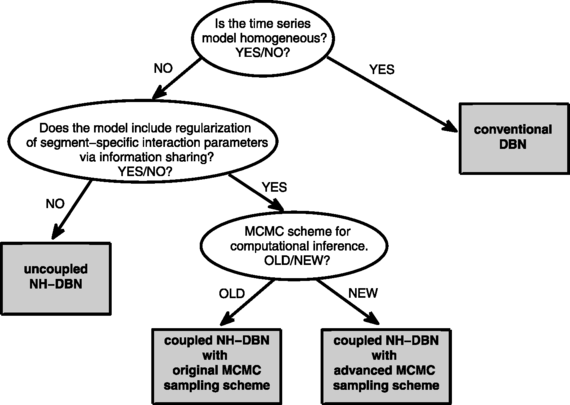

  

  Graphical tree representation of the four methods under comparison. The four methods are represented as gray rectangles. In our empirical study we compare three DBN models: A conventional homogeneous DBN, an uncoupled non-homogeneous DBN akin to Lèbre et al. (2010), and the proposed non-homogeneous globally coupled NH-DBN. For the proposed globally coupled NH-DBN we also compare the original MCMC sampling scheme from Grzegorczyk and Husmeier (2012b) and the advanced MCMC sampling scheme from Sect. 2.2.4, proposed here. See Table 5 for more details on the four methods

  Table 5 Overview of the four methods under comparison. The conventional dynamic Bayesian network (DBN) model is homogeneous and assumes that the interaction parameters are constant and do not change over time. The non-homogeneous DBN (NH-DBN) models allow for changepoints that divide the time series into segments and for each segment there are segment-specific interaction parameters. Unlike the uncoupled NH-DBN model the coupled NH-DBN model allows for global information sharing (i.e. coupling) between the segment-specific interaction parameters. The coupled NH-DBN model can be inferred with two different MCMC sampling schemes. See Fig. 5 for a graphical representation of the relationships between the four methods

• In Sect. 5.2 we employ gene expression time series from Saccharomyces cerevisiae (see Sect. 3.2) to extend our comparative evaluation by a real-world application. As in the first study we evaluate the network reconstruction accuracy for different hyperparameter settings, we cross-compare the performance of the two MCMC sampling schemes, and we impose the constraints g∉π _g (g=1,…,N). But unlike in the first study we assume the segmentations (changepoint sets) to be unknown. The node-specific changepoint sets $\mbox {{\boldmath $\tau $}}_{g}$ (g=1,…,N) have to be inferred from the data and the network reconstruction accuracy can be monitored in dependence on the inferred segmentations. In Sect. 5.2.2 we extend our cross-method comparison and empirically compare the proposed globally coupled NH-DBN with a sequentially coupled NH-DBN model, presented in Grzegorczyk and Husmeier (2012a), with respect to the network reconstruction accuracy.

• In Sect. 5.3 we analyze gene expression time series from Arabidopsis thaliana (see Sect. 3.3). For the Arabidopsis thaliana data a proper evaluation in terms of the network reconstruction accuracy is infeasible owing to the absence of a proper gold standard. Several authors aim to pursue an evaluation without gold standard by arguing for the biological plausibility of subsets of inferred interactions. However, such an approach inevitably suffers from a certain selection bias and is somewhat subject to subjective interpretation. Our primary focus is therefore on quantifying the strength of the information coupling between the time series segments and the influence this coupling has on the regulatory network reconstruction. We compute and compare the correlations between the segment-specific interaction parameter vectors for the uncoupled and for the coupled NH-DBN. For comparing the correlations of the two NH-DBN models we require an invariant segmentation. Since there are four individual time series, which have been measured under different external conditions, as indicated in Table 4, a natural choice is to consider each of the four individual time series as a separate segment. In this third application we do not rule out self feedback loops, i.e., we allow for g∈π _g (g=1,…,N), since—from a biological perspective—self feedback loops cannot be excluded for the underlying gene regulatory network.

4.2 Hyperparameter settings for the coupled NH-DBN model and the competing methods

We assume that the gene-specific variances are shared by all segments: $\sigma_{g,h}^{2}=\sigma_{g}^{2}$. According to (30) the prior distributions of the node-specific inverse variance hyperparameters, $\sigma_{g}^{-2}$ (g=1,…,N), are assumed to be Gamma distributions with level-2 hyperparameters A _σ and B _σ . Except for an analysis where we directly fix the two level-2 hyperparameters (see Sect. 5.1), we set A _σ =0.005:

$$\sigma_g^{-2} \sim \operatorname {Gam}(A_{\sigma}=0.005,B_{\sigma}) $$

and impose the level-3 Gamma prior from (32) on B _σ

$$B_{\sigma} \sim \operatorname {Gam}(\alpha_{\sigma}, \beta_{\sigma}) $$

For the latter pair of level-3 hyperparameters we employ three settings, namely: (α _σ ,β _σ )∈{(1,200),(0.1,20),(0.01,2)}, such that we obtain for the level-3 prior distribution: $E[B_{\sigma}]=\frac{\alpha_{\sigma}}{\beta_{\sigma}}=0.005$.¹¹ The prior variance of B _σ depends on the level-3 hyperparameters: Low level-3 hyperparameters correspond to weak (vague, uninformative) prior distributions, which do not force B _σ ≈0.005 and thus allow for more flexibility, as the posterior distribution of B _σ depends on the data more strongly then.

From (31) it can be seen that the node-specific signal-to-noise hyperparameters, δ _g (g=1,…,N), are assumed to be Gamma distributed with level-2 hyperparameters A _δ and B _δ . Except for the analysis in Sect. 5.1 and in Sect. 5.2.2, where we directly fix all the level-2 hyperparameters, we fix A _δ =2 and use the level-3 Gamma prior from (33) for B _δ

$$\delta_g^{-1} \sim \operatorname {Gam}(A_{\delta}=2,B_{\delta}), \quad B_{\delta} \sim \operatorname {Gam}(\alpha_{\delta},\beta_{\delta}) $$

and we employ four different settings for the latter pair of level-3 hyperparameters, namely: (α _δ ,β _δ )∈{(200,1000),(20,100),(2,10),(0.2,1)}, such that we obtain for the prior distribution: $E[B_{\delta}]=\frac{\alpha_{\delta}}{\beta_{\delta}}=0.2$.¹² The prior variance of B _δ depends on the level-3 hyperparameters¹³: The high values for the level-3 hyperparameters (e.g. α _δ =200 and β _δ =1000) lead to strong (informative, concentrated) prior distributions, which force B _δ ≈0.2, while the low values for the level-3 hyperparameters allow for more flexibility and lead to weak (diffuse, vague) prior distributions.

The gene- and segment-specific interaction parameter vectors w _g,h are assumed to be multivariate Gaussian distributed according to (11), and in the absence of any genuine prior knowledge we set C _g,h =I.

In the uncoupled NH-DBN the global hyperparameter vectors are fixed, m _g =0 ∀g, and with $\sigma_{g,h}^{2}=\sigma_{g}^{2}$, it follows from (11): $\mathbf {w}_{g,h}|(\mathbf {m}_{g}=\mathbf{0},\sigma_{g}^{2},\delta_{g}) \sim\mathcal{N}(\mathbf{0},\delta_{g} \sigma^{2}_{g}\mathbf{I})$. For the proposed coupled NH-DBN model the node-specific global hyperparameter vectors m _g (g=1,…,N) are flexible, with the prior distribution given in (12):

$$\mathbf {m}_{g} \sim\mathcal{N}(\mathbf {m}_{\dagger}, \boldsymbol {\varSigma }_{\dagger}) $$

and we set m _†=0 and S _†=I.

In our first empirical study in Sect. 5.1 we also compare the performance of the two NH-DBN models with the conventional homogeneous DBN, which is a special case of our model with an empty non-adaptable changepoint set.

For the analysis of the Saccharomyces cerevisiae gene expression time series in Sect. 5.2 we follow an unsupervised approach and assume that the changepoints segmenting the time series are unknown. To infer different segmentations we employ different hyperparameters of the point process prior on the changepoint sets. In the point process prior, described in Sect. 2.2.2, the prior distribution for the number of time points between two successive changepoints is a negative binomial distribution with hyperparameters k and p. In the probability mass function of the negative binomial distribution, given in (36), we fix k=1 and vary the hyperparameter p over a wide range of values: p∈{0,0.001,0.005,0.01,0.02,0.03,0.04,0.1,0.2,0.3,0.4}.

In our last empirical study in Sect. 5.2 we compare the performance of the two NH-DBN models with a sequentially coupled NH-DBN model, proposed in Grzegorczyk and Husmeier (2012a). For this study we re-use the hyperparameter values from Grzegorczyk and Husmeier (2012a). A brief description of the sequentially coupled NH-DBN can be found in Sect. 4 of Online Resource 2.

4.3 MCMC simulation lengths, convergence diagnostics and criterions for the network reconstruction accuracy

For the comparison of the methods shown in Fig. 5 and Table 5 we have to perform (partially collapsed Gibbs) MCMC simulations, as described in Sects. 2.2.3 and 2.2.4, and we proceed as follows: After the burn-in phase of 5,000 (5k) MCMC iterations, we perform 5k MCMC iterations in the sampling phase, in which we sample in equidistant intervals (every 100-th iteration) to obtain a network sample $\mathcal{M}^{(1)},\ldots ,\mathcal{M}^{(50)}$ of size 50. From the network sample we compute the marginal edge posterior probabilities. For a network with N nodes an estimator e _n,j for the marginal posterior probability of the individual edge from node n to node j is given by:

$$ e_{n,j} = \frac{1}{50} \sum _{i=1}^{50} \mathcal{M}^{(i)}(n,j) $$

(51)

where $\mathcal{M}^{(i)}(n,j)$ is an indicator function which is 1 if the i-th network in the sample, $\mathcal{M}^{(i)}$, contains the edge n→j, and 0 otherwise (n,j∈{1,…,N}).

To assess convergence and mixing we applied standard convergence diagnostics, based on trace plots (Giudici and Castelo 2003) and the potential scale reduction factor (Gelman and Rubin 1992), and found that the PSRF’s of all individual edges were below 1.1 for simulation lengths of 10,000 MCMC steps, when the advanced MCMC sampling scheme is used. More details and in particular details on how we defined a PSRF for an individual network edge can be found in Sect. 3 of Online Resource 1.

If the true network is known, we evaluate the network reconstruction accuracy in terms of the areas under the receiver operator characteristic curve (AUC-ROC) and in terms of the areas under the precision recall curve (AUC-PR). Details on these two criterions can be found in Sect. 3 of Online Resource 1.

5 Results

5.1 Results on simulated data from the RAF pathway

We take the RAF network from Sachs et al. (2005), see Fig. 3, and generate synthetic non-homogeneous time series from a multiple changepoint linear regression model, as explained in Sect. 3.1. Our objective is to monitor the network reconstruction accuracy on a series of increasingly strong violations of the prior assumption inherent in (11)–(12).

5.1.1 Comparative evaluation between three DBN models for fixed level-2 and level-3 hyperparameters and flexible SNR

In a first step we select the level-3 hyperparameters such that the level-2 hyperparameters are equal in prior expectation to those imposed in earlier studies for simpler versions of these NH-DBN models without level-3 hyperpriors (see, e.g., Grzegorczyk and Husmeier 2012b).¹⁴ We cross-compare the performance of the conventional homogeneous DBN, the uncoupled NH-DBN akin to Lèbre et al. (2010), and the proposed coupled NH-DBN; see Fig. 5 and Table 5 in Sect. 4.

The empirical results are shown in Fig. 6. For the low signal-to-noise ratio (SNR=1) there is no significant difference between the three dynamic Bayesian network models. However, owing to the high noise level, the network reconstruction accuracy is close to random expectation (AUC-ROC=0.5) in that case. For high (SNR=10) and moderate (SNR=3) noise levels, the proposed coupled NH-DBN outperforms the homogeneous DBN and the uncoupled NH-DBN. That is, the proposed model does not perform worse than the homogeneous DBN if the data are homogeneous (ϵ=0 in Fig. 6), while the proposed model increasingly outperforms the conventional homogeneous DBN as the amplitude of the perturbation ε of the parameter vectors increases (ϵ>0 in Fig. 6). Conversely, the proposed coupled NH-DBN increasingly outperforms the uncoupled NH-DBN as the amplitude of the perturbation ε of the parameter vectors decreases. In particular, except for the strongest perturbation (ε=1) the performance improvement of the proposed coupled NH-DBN over the uncoupled NH-DBN is significant.

Fig. 6

Network reconstruction (in terms of mean AUC-ROC scores) for the RAF network from simulated expression data. The figure monitors the network reconstruction accuracy in terms of AUC-ROC scores for the conventional homogeneous DBN (DBN; dotted black lines), the uncoupled non-homogeneous DBN (uncoupled NH-DBN; solid gray lines) and the proposed coupled non-homogeneous DBN (coupled NH-DBN; solid black lines) and demonstrates how the proposed regularization scheme is affected by increasing violations of the prior assumption inherent in (11)–(12). We imposed the following (hyper-)prior distributions: $\sigma_{g}^{-2}\sim \operatorname {Gam}(0.005,B_{\sigma})$ with $B_{\sigma}\sim \operatorname {Gam}(1,200)$ and $\delta_{g}^{-1}\sim \operatorname {Gam}(2,B_{\delta})$ with $B_{\delta}\sim \operatorname {Gam}(200,1000)$. Simulated data were generated as described in Sect. 3.1. The global parameter vector with amplitude 1 was perturbed in a segment-wise manner by a random perturbation of amplitude ε (abscissa); see (49). The columns represent the three SNR levels 10, 3, and 1. The top row shows the absolute values of the mean AUC-ROC scores, while the bottom rows show the differences between the proposed coupled NH-DBN and the standard homogeneous DBN (center row) and the uncoupled NH-DBN (lower row). All simulations were repeated on 25 independent data instantiations, with error bars indicating two-sided 95 % confidence intervals. A similar plot with AUC-PR scores is provided in Online Resource 3 (see Fig. 1)

Since the network reconstruction accuracy is close to random expectation for the high noise level (SNR=1) and almost identical for the low (SNR=10) and the moderate (SNR=3) noise level, we focus our attention on the latter in the following subsections.

5.1.2 Comparison of three different coupling schemes for the noise variance hyperparameters

Six coupling schemes (S1)–(S9) for the noise variance hyperparameters, $\sigma_{g,h}^{2}$, were briefly outlined in Table 2 in Sect. 2.2.1. Throughout this paper we focus on coupling scheme (S8): “weak coupling for nodes, hard coupling for segments”, but in this subsection we briefly compare this scheme with two alternative schemes, namely the (S4) approach: “no coupling for nodes, weak coupling for segments” and the (S5) approach: “weak coupling for both nodes and segments”. For this study we re-use the hyperprior from Sect. 5.1.1 for the signal-to-noise hyperparameters, δ _g (g=1,…,N), and we vary the level-3 hyperparameters for the noise variance hyperparameters, $\sigma_{g}^{2}$ or $\sigma_{g,h}^{2}$, respectively.¹⁵ The technical details and figures of the empirical results have been relegated to Sect. 3 of Online Resource 2. Here we just briefly summarize our findings for the RAF pathway data with SNR=3: In a comparative evaluation of the three approaches (S4), (S5), and (S8) for the proposed coupled NH-DBN model we found that the coupled NH-DBN yields consistently the best network reconstruction accuracy when coupling scheme (S8) is employed; see Figs. 7–8 in Sect. 3 of Online Resource 2. Moreover, for each of the three coupling schemes (S4), (S5), and (S8) we found that the proposed coupled NH-DBN model compares favorably to the uncoupled NH-DBN model akin to Lèbre et al. (2010); see Figs. 9–10 in Sect. 3 of Online Resource 2. In particular for (S4), (S5) and (S8) exactly the same trend can be observed: Except for the strongest amplitude of the perturbation (ε=1) the performance improvement of the proposed coupled NH-DBN over the uncoupled NH-DBN is significant and the relative AUC-ROC and AUC-PR differences increase as the amplitude, ε, decreases. Our empirical findings thus suggest that the merits of the proposed coupled NH-DBN model do not depend on the coupling scheme for the noise variance hyperparameters.

5.1.3 Robustness with respect to the level-2 hyperparameters

In the third step we focus on cross-comparing the uncoupled and the coupled NH-DBN model and we investigate whether the trends from Sect. 5.1.1 can also be found for other hyperparameter settings. For this analysis we return to the simpler NH-DBN models without level-3 hyperpriors (Grzegorczyk and Husmeier 2012b). That is, we directly fix the level-2 hyperparameters in (30)–(31), and we re-analyze the synthetic RAF network data with SNR=3 with the two NH-DBN models.¹⁶ Figures of the empirical results have been relegated to Sect. 1 of Online Resource 2 and can be summarized as follows. In consistency with the results from Sect. 5.1.1, the proposed coupled DBN increasingly outperforms the uncoupled NH-DBN as the amplitude of the perturbation ε of the parameter vectors decreases (see Figs. 1–2 in Sect. 1 of Online Resource 2). Our data analysis not only shows that the relative differences in the network reconstruction accuracy are in favor of the proposed coupled NH-DBN but also reveal that the network reconstruction accuracy, measured in terms of mean AUC-ROC scores, is robust with respect to the choices of the level-2 hyperparameters. As shown in Fig. 3 of Online Resource 2, the proposed coupled NH-DBN yields almost identical AUC-ROC scores for each of the 12 level-2 hyperparameter settings.

5.1.4 Robustness with respect to the level-3 hyperparameters

In the fourth step we return to the more flexible NH-DBN models with level-3 hyperpriors. Since we have seen in Sect. 5.1.3 that the models are fairly robust with respect to different choices of the level-2 hyperparameters, we now fix the level-2 hyperparameters A _σ and A _δ in (30)–(31) and we focus on the level-3 hyperparameters in (32)–(33).¹⁷ We re-analyze the synthetic RAF network data with SNR=3 for 12 settings of the level-3 hyperparameters in (32)–(33). For the coupled NH-DBN we employ the advanced MCMC sampling scheme from Sect. 2.2.4. Figure 7 monitors the average AUC-ROC scores for these hyperparameter settings, and it can be seen that the level-3 hyperprior on B _σ has only a minor effect on the performance of the models, while the level-3 hyperprior on B _δ seems to be important. In consistency with our earlier findings (see, e.g., bottom rows of Figs. 1–2 in Online Resource 2) Fig. 8 reveals that the coupled NH-DBN compares favorably to the uncoupled NH-DBN for the two stronger priors on B _δ , while the advantage appears to diminish for the two weak priors. For the two strong priors the coupled NH-DBN yields significantly greater AUC-ROC scores than the uncoupled NH-DBN, unless the amplitude of the perturbation reaches the highest level (ϵ=1). On the other hand, for the two weak priors the proposed coupled NH-DBN performs better only for low amplitudes of the perturbation (ϵ=0 and ϵ=1/8), while the performance of the coupled NH-DBN becomes even slightly worse than the performance of the uncoupled NH-DBN for high amplitudes of the perturbation (ϵ=1/2 and ϵ=1), where in particular for ϵ=1/2 the difference appears to be significant in favor of the uncoupled NH-DBN (see, e.g., bottom right panel of Fig. 8). We discuss the reasons for this trend in Sect. 5.1.7.

Fig. 7

Sensitivity of network reconstruction accuracy (in terms of mean AUC-ROC scores) for the synthetic RAF network data with SNR=3. Systematic variation of the level-3 hyperparameters in (32)–(33). Comparative evaluation of the uncoupled and the coupled NH-DBN. The figure is arranged as a 4-by-3 matrix, where the columns correspond to three different level-3 hyperpriors for B _σ (see (32) with A _σ =0.005) and the rows correspond to four different level-3 hyperpriors for B _δ (see (33) with A _δ =2). In each panel we monitor the network reconstruction accuracy in terms of AUC-ROC scores for the uncoupled NH-DBN (solid gray lines) and the coupled NH-DBN with the advanced MCMC sampling scheme from Sect. 2.2.4 (solid black lines). Simulated data were generated as described in Sect. 3.1. The global parameter vector with amplitude 1 was perturbed in a segment-wise manner by a random perturbation of amplitude ε (abscissa); see (49). The panels show the absolute values of the mean AUC-ROC scores. All simulations were repeated on 25 independent data instantiations. A similar plot with AUC-PR scores is provided in Online Resource 3 (see Fig. 5)

Fig. 8

Mean AUC-ROC differences between the coupled and the uncoupled NH-DBN model for the synthetic RAF network data with SNR=3. Systematic variation of the level-3 hyperparameters in (32)–(33). The figure is arranged as a 4-by-3 matrix, where the columns correspond to three different level-3 hyperpriors for B _σ (see (32) with A _σ =0.005) and the rows correspond to four different level-3 hyperpriors for B _δ (see (33) with A _δ =2). In each panel we monitor the mean AUC-ROC differences between the proposed coupled NH-DBN (inferred with the advanced MCMC sampling scheme from Sect. 2.2.4) and the uncoupled NH-DBN. For details on the data sets see the caption of Fig. 7. A similar plot with AUC-PR scores is provided in Online Resource 3 (see Fig. 6)

5.1.5 Posterior distribution of the signal-to-noise hyperparameter in dependence on the level-3 hyperparameters

We want to find the reason why the coupled NH-DBN does not perform better than the uncoupled NH-DBN for weak priors on B _δ (see Figs. 7–8). To this end, we explore the posterior distribution of the signal-to-noise hyperparameters, δ _g . Since our findings in Sect. 5.1.4 suggest that the two models appear to be robust with respect to a variation of the level-3 hyperprior on B _σ , we employ the weakest (most diffuse) prior for B _σ , $B_{\sigma }\sim \operatorname {Gam}(0.01,2)$.

Histograms of the posterior distribution of log(δ _g ) for the uncoupled NH-DBN with four different level-3 hyperpriors on B _δ can be found in Online Resource 2 (see Fig. 4). The level-3 hyperparameters have a moderate effect on the posterior variance, i.e., for the weaker priors the posterior distributions are slightly stronger peaked. The amplitude of the perturbation, ϵ, seems to have no effect on the posterior distribution of δ _g . This latter finding is not surprising, since the uncoupled NH-DBN learns the interaction parameters independently for each segment, and it thus does not matter whether the segment-specific interaction parameter vectors are similar or not. For the uncoupled NH-DBN the posterior distribution of δ _g depends on the amplitudes of the interaction parameter vectors only. And independently of the amplitude of the perturbations, ϵ, the amplitudes of the interaction parameter vectors are always equal to 1 in this particular application.

Histograms of the posterior distribution of log(δ _g ) for the coupled NH-DBN (inferred with the advanced MCMC sampling scheme) for four different level-3 hyperpriors on B _δ are given in Fig. 9. Unlike the findings for the uncoupled NH-DBN, the posterior distribution of δ _g now depends on both: the level-3 hyperpriors on B _δ and the amplitude of the perturbations, ϵ. For the two strong priors on B _δ (see top rows in Fig. 9) a plausible trend can be observed. With increasing amplitude of the perturbations, ϵ, the similarity between the interaction parameter vectors gets lost and thus the signal-to-noise hyperparameters, δ _g , increase (i.e. the coupling strengths, $\delta_{g}^{-1}$, get weaker). For the two weak priors on B _δ (see bottom rows in Fig. 9) the signal-to-noise hyperparameters, δ _g , take on extremely low values of log(δ _g )≈−75. The corresponding coupling strengths, $\delta_{g}^{-1}$ with $\log(\delta_{g}^{-1})\approx75$, are consistent with homogeneous (ϵ=0) or quasi-homogeneous (ϵ≈0) data.¹⁸ They are inconsistent with higher amplitudes of the perturbation, ϵ>0, i.e., data that have been generated with non-homogeneous segment-specific interaction parameter vectors. However, Fig. 9 reveals that up to ϵ=0.5 most of the sampled signal-to-noise hyperparameters δ _g take on this extreme value, log(δ _g )≪0, and that it is only avoided as the amplitude of the perturbation reaches its maximum value of ϵ=1.

Fig. 9

Posterior distribution of the (logarithmic) signal-to-noise ratio hyperparameter, log(mean(δ _g )), for the proposed coupled NH-DBN model, averaged over the 25 RAF pathway data sets with SNR=3. The figure is arranged as a matrix, where the rows correspond to the level-3 hyperprior on B _δ (see (31) and (30) with A _δ =2), and the columns correspond to the amplitude, ϵ, of the perturbation with which the global parameter vector was perturbed (see Sect. 3.1 for details). The advanced MCMC sampling scheme from Sect. 2.2.4 was used for inference. Each histogram was obtained by merging the signal-to-noise hyperparameters, δ _g , which were sampled after the burn-in phase of 5,000 MCMC iterations, of all genes, g, from the 25 data instantiations. For the hyperpriors on the noise variances, $\sigma_{g}^{2}$, we set A _σ =0.005 in (30) and α _σ =0.01 and β _σ =2 in (32)

As a complementary analysis, Fig. 5 in Online Resource 2 shows overlaid trace plots of the signal-to-noise hyperparameters during the sampling phase (i.e., from iteration 5k to iteration 10k (with k=1,000)), from which the histograms in Fig. 9 have been extracted. The graphs indicate that the extreme signal-to-noise hyperparameter value, log(δ _g )≪0, observed for weak priors on B _δ , is an attractor state, i.e., a state that the MCMC trajectory can converge to, but never leave. We note that the occurrence of such inconsistent absorbing states in Bayesian hierarchical models as a consequence of weak priors was briefly mentioned in Andrieu and Doucet (1999), p. 2673. We will discuss this point in more detail in Sect. 5.1.7.

5.1.6 Comparison of the two MCMC sampling schemes for the coupled NH-DBN model

In this subsection we cross-compare the performance of the original MCMC sampling scheme from Grzegorczyk and Husmeier (2012b) and the advanced MCMC sampling scheme, proposed here (see Sect. 2.2.4); see Fig. 5 for an overview. To this end, we re-analyze the RAF pathway data with SNR=3 with the original MCMC sampling scheme. We have already seen in Sect. 5.1.4 that weak priors for B _δ lead to attractor states with extreme values for the signal-to-noise hyperparameters, δ _g . We suggest that these absorbing attractor states might also be responsible for the low network reconstruction accuracy (AUC-ROC values) of the original MCMC sampling in the bottom rows of Fig. 7. For each amplitude of the perturbation, ϵ∈{0,0.125,0.25,0.5,1}, we therefore randomly selected five synthetic RAF pathway data sets, i.e. 25 individual data sets in total, and for each individual data set we assessed convergence of the three NH-DBN methods from Fig. 5 and Table 5. We consider a strong prior and a weak prior on B _δ .¹⁹ With each of the three NH-DBN methods and each of the two priors on B _σ we performed H=5 independent MCMC simulations for each of the 25 individual data sets. We assessed convergence and mixing by computing the potential scale reduction factors (PSRFs) from the marginal posterior probabilities of the network edges, as described in detail in Sect. 3 of Online Resource 1.

Figure 10 shows the network reconstruction accuracy results obtained for the five different ϵ values. Figure 11 monitors the average fractions of individual network edges for which the target convergence level PSRF<1.1 has been reached, for the number of MCMC iterations.²⁰ The uncoupled NH-DBN and the proposed coupled NH-DBN with the advanced MCMC sampling scheme from Sect. 2.2.4 converge for both priors and each of the five amplitudes ϵ, while the proposed coupled NH-DBN with the original MCMC sampling scheme does not always reach the target convergence level. When the weak prior on B _δ is employed (see bottom row in Fig. 11) the latter method completely fails to reach the target convergence level, unless the amplitude of the perturbation, ϵ, is equal to 1. Moreover, the original MCMC sampling scheme also converges significantly slower than the other two methods for the strong prior when ϵ≤0.25 (see first three panels in the top row of Fig. 11). We will discuss this point in more detail in Sect. 5.1.7.

Fig. 10

Sensitivity of network reconstruction accuracy (in terms of mean AUC-ROC scores) for the synthetic RAF network data with SNR=3. Systematic variation of the level-3 hyperparameters in (32)–(33). Comparative evaluation of the two MCMC sampling schemes for the coupled NH-DBN model. The figure is arranged as a 4-by-3 matrix, where the columns correspond to three different level-3 hyperpriors for B _σ (see (32) with A _σ =0.005) and the rows correspond to four different level-3 hyperpriors for B _δ (see (33) with A _δ =2). In each panel we monitor the network reconstruction accuracy in terms of AUC-ROC scores for the coupled NH-DBN with the original MCMC sampling scheme (dotted gray lines) and the coupled NH-DBN with the advanced MCMC sampling scheme from Sect. 2.2.4 (solid black lines). Simulated data were generated as described in Sect. 3.1. The global parameter vector with amplitude 1 was perturbed in a segment-wise manner by a random perturbation of amplitude ε (abscissa); see (49). The panels show the absolute values of the mean AUC-ROC scores. All simulations were repeated on 25 independent data instantiations. A similar plot with AUC-PR scores is provided in Online Resource 3 (see Fig. 7)

Fig. 11

Convergence diagnostics based on the potential scale reduction factors (PSRFs) of individual network edges—Synthetic RAF pathway data with SNR=3. We compare the convergence of (i) the uncoupled NH-DBN (solid gray lines), (ii) the proposed coupled NH-DBN with the original MCMC sampling scheme described in Sect. 2.2.3 (dotted black lines), and (iii) the proposed coupled NH-DBN with the advanced MCMC sampling scheme from Sect. 2.2.4 (solid black lines). The five columns correspond to the amplitude, ϵ, of the perturbation with which the global hyperparameter vector was perturbed (see Sect. 3.1 for details). In the top row we employed a strong prior ($B_{\delta}\sim \operatorname {Gam}(20,100)$ in (33)) and in the bottom row we employed a weak prior ($B_{\delta}\sim \operatorname {Gam}(0.2,1)$ in (33)) for B _δ , while we set A _δ =2 in (31). For each individual network edge a PSRF was computed, and the panels show trace plots of the fractions of individual network edges whose PSRF was lower than the standard threshold PSRF<1.1 (vertical axis) monitored along the number of MCMC iterations (horizontal axis). The results displayed in the panels are mean fractions averaged over 5 individual data instantiations of the RAF-pathway; each analyzed H=5 times with the three methods under comparison. For the level-3 hyperpriors on the noise variance hyperparameters, $\sigma_{g}^{2}$, we set A _σ =0.005 in (30) and α _σ =0.01 and β _σ =2 in (32). Details on how we defined the PSRF for an individual network edge can be found in Sect. 3 of Online Resource 1

5.1.7 Discussions of the results for the RAF pathway data

In this subsection we provide a theoretical explanation of two empirical findings. First, we explain why weak (vague) level-3 hyperpriors on B _δ are disadvantageous for the proposed coupled NH-DBN. Second, we explain why the advanced MCMC sampling scheme converges substantially better than the original MCMC sampling scheme from Grzegorczyk and Husmeier (2012b).

The disadvantage of weak (diffuse) priors on B _δ

In Sect. 5.1.4 we found that the network reconstruction accuracy of the coupled NH-DBN model tends to be superior to that of the uncoupled NH-DBN model unless we use a weak prior on B _δ and a medium amplitude of the perturbation, ϵ=0.5; see e.g. Fig. 8. The reason for this behavior becomes clear from the existence of an absorbing state with very low signal-to-noise value, log(δ _g )≪0, which was already discussed in Sect. 5.1.4 and is illustrated in the two bottom rows of Fig. 9. For this absorbing state, the prior and posterior distributions of the segment-specific interaction parameters, w _g,h , become highly peaked around the global hyperparameter vector, m _g ; see (11) and (27).²¹ Mathematically, w _g,h converges in distribution to m _g as δ _g →0: w _g,h →m _g (h=1,…,K _g ) for δ _g →0, and the coupled NH-DBN reduces to a conventional homogeneous DBN. We can thus distinguish three regimes for the perturbation amplitude, ϵ. For zero (ϵ=0) or very small perturbations (0<ϵ≪1), the data are adequately modeled with a homogeneous DBN, and by reducing to this model, the coupled NH-DBN outperforms the uncoupled one. For intermediate amplitudes of the perturbation, ϵ=0.5, the data are not adequately modeled by a homogeneous DBN, the attractor state is inconsistent with the data, and by reducing to the homogeneous DBN, the coupled DBN is outperformed by the uncoupled one. For large noise amplitudes, ϵ=1, the attractor state is avoided, and the coupled NH-DBN no longer reduces to the homogeneous one. However, due to the large perturbation there is not much benefit in using any information sharing among segments, and the coupled and uncoupled NH-DBN show approximately equal performance.

As seen from the top rows of Fig. 8, effective information coupling for quasi-homogeneous data can be accomplished with less extreme values of δ _g than those of the absorbing state, while entrapment in the absorbing state is detrimental to the performance in the medium perturbation regime around ϵ≈0.5. For that reason, it is advisable to prevent such entrapment. Our results, shown in Fig. 9, suggest that this can be effected by the use of a sufficiently strong (informative, concentrated) prior on B _δ .

The advantage of the advanced MCMC sampling scheme

In Sect. 5.1.6 we found that the advanced MCMC sampling scheme, proposed here, converges substantially better than the original MCMC sampling scheme from Grzegorczyk and Husmeier (2012b); see Fig. 11. The convergence improvement that can be reached with the advanced MCMC sampling scheme, can be explained as follows: We assume that the Markov chain has reached a parent node set $\pi_{g}^{(i)}$, the global interaction hyperparameter vector $\mathbf{m}_{g}^{(i)}$, and the signal-to-noise hyperparameter, $\delta_{g}^{(i)}$. Adding a new parent node to the current parent set, $\pi_{g}^{(i)}$, yields a new parent set $\pi_{g}^{(\diamond)}$ and the corresponding new global interaction hyperparameter vector, $\mathbf{m}_{g}^{(\diamond)}$, requires a new component for the new parent node. Unlike the original MCMC sampling scheme, which only samples the new component of $\mathbf {m}_{g}^{(\diamond)}$ according to its prior distribution (see (12)), the advanced MCMC sampling scheme re-samples the whole global hyperparameter vector, $\mathbf {m}_{g}^{(\diamond)}$, conditional on the new parent set, $\pi_{g}^{(\diamond )}$, according to its posterior distribution in (46). That is, the segment-specific interaction parameters for the new parent set are centered around the new vector, $\mathbf {m}_{g}^{(\diamond)}$, which either contains an a priori sampled entry (original MCMC) or is an a posteriori sample (advanced MCMC). That is, unlike the original MCMC sampling scheme, the advanced MCMC sampling scheme guarantees that the distributions of the segment-specific interaction parameters are centered around an a posteriori sample $\mathbf {m}_{g}^{(\diamond)}$, and thus ensures that the marginal likelihoods and the acceptance probabilities are higher.²² In particular, as discussed above, weak priors on B _δ can lead to attractor states with extremely low values for the signal-to-noise hyperparameters, $\delta_{g}^{(i)}$. For $\delta_{g}^{(i)}\rightarrow0$ the posterior distributions of the segment-specific interaction parameters, w _g,h , are not only centered but peaked²³ around the global hyperparameter vector, $\mathbf{m}_{g}^{(\diamond)}$; see (27), and the marginal likelihoods (acceptance probabilities) for the original MCMC sampling scheme, for which $\mathbf {m}_{g}^{(\diamond)}$ contains an a priori sampled entry, can become very low.

5.2 Gene regulation in Saccharomyces cerevisiae

5.2.1 Performance of the coupled NH-DBN model

In this subsection we compare the three NH-DBN methods (see Fig. 5 and Table 5) on the gene expression profiles from Saccharomyces cerevisiae, described in Sect. 3.2. Here we also know the true regulatory network, shown in Fig. 4, so that we can objectively cross-compare the network reconstruction accuracy on real biological data. Unlike our earlier data analysis in Sect. 5.1 we now follow an unsupervised approach and assume the segmentations (changepoint sets) to be unknown. That is, the changepoint sets have to be inferred from the data. To obtain different data segmentations we run MCMC simulations (with 10k iterations each) for various hyperparameters of the point process prior on the changepoint locations. As described in Sect. 2.2.2, the distance between changepoints is assumed to follow a negative binomial distribution, and we use the hyperparameters k=1 and p∈{0,0.001,0.01,0.02,0.03,0.04,0.1,0.2,0.3,0.4} in (36).

For the synthetic RAF pathway data we found in Sect. 5.1 that the three methods are robust with respect to a variation of the level-3-hyperparameters for the hyperprior on B _σ , and we therefore use the weakest prior on B _σ .²⁴ For the level-3 hyperparameters on B _δ we again choose four different settings.²⁵

Figure 12 shows the average AUC-ROC scores plotted against the average number of changepoints per gene,²⁶ $\overline {K}$, for the four level-3 hyperpriors on B _δ . It is clearly seen from the top row in Fig. 12 that the proposed coupled NH-DBN yields a systematically better network reconstruction accuracy than the uncoupled NH-DBN for the two strong priors on B _δ and that the two MCMC sampling schemes (from Sects. 2.2.3 and 2.2.4) for the coupled NH-DBN model perform approximately equally well. For $B_{\delta}\sim \operatorname {Gam}(200,1000)$ and $B_{\delta}\sim \operatorname {Gam}(20,100)$ the best performance of the novel coupled NH-DBN is given for $\overline {K}\approx1$, which reflects the imposed environment change related to the switch of the carbon source from galactose to glucose. $\overline {K}=0$ corresponds to the conventional homogeneous DBN, for which the network reconstruction is significantly worse. Much larger average numbers of changepoints $\overline {K}$ render the model over-flexible, which is reflected by a decline in the AUC-ROC scores. Interestingly, this decline is less pronounced for the proposed coupled NH-DBN model than for the uncoupled NH-DBN model, indicating increased robustness with respect to a variation of the prior assumptions on the time series segmentation.

Fig. 12

Gene network reconstruction accuracy in terms of AUC-ROC scores for the Saccharomyces cerevisiae data. The graphs show the network reconstruction accuracy (ordinate) plotted against the mean number of changepoints per gene (abscissa) for the uncoupled NH-DBN (solid gray line), the proposed coupled NH-DBN with the original MCMC sampling scheme from Sect. 2.2.3 (dotted black line), and the proposed coupled NH-DBN with the advanced MCMC sampling scheme from Sect. 2.2.4 (solid black line). The results have been obtained with four different level-3 hyperpriors on B _δ , see (33), as indicated on the top of each panel. In (31) we set A _δ =2, and for the level-3 hyperpriors of the noise variance hyperparameters, $\sigma_{g}^{2}$, we set A _σ =0.005 in (30) and α _σ =0.01 and β _σ =2 in (32). The network reconstruction accuracy is quantified in terms of mean AUC-ROC scores, averaged over 5 MCMC simulations, with the vertical bars indicating standard errors. A similar plot with AUC-PR scores is provided in Online Resource 3 (see Fig. 8)

For the two weak priors on B _δ in the bottom row of Fig. 12 the network reconstruction accuracy (measured in terms of AUC-ROC scores) for all three methods is substantially worse than for the stronger priors. Although the coupled NH-DBN model still performs better than the uncoupled NH-DBN model it appears that its performance does not depend on the average number of changepoints. That is, independently of the inferred average number of changepoints $\overline {K}$ the mean AUC-ROC values of the coupled NH-DBN model are not better than the AUC-ROC values of a conventional homogeneous DBN without changepoints ($\overline {K}=0$). In consistency with those findings reported for the synthetic RAF pathway data in Sect. 3.1 it can also be seen from the bottom row in Fig. 12 that the advanced MCMC sampling performs (at least slightly) better than the original MCMC sampling scheme for the two weak priors on B _δ .

Figure 13 shows some trace plot diagnostics of the coupled NH-DBN model (inferred with the advanced MCMC sampling scheme) for the first 500 MCMC iterations. The first column shows overlaid trace plots of the sampled signal-to-noise hyperparameters, $\delta_{g}^{(i)}$ (g=1,…,5), the second column monitors the posterior samples of $B_{\delta}^{(i)}$, and the third column monitors the average Euclidean distances between the segment-specific interaction parameter vectors, w _g,h , and the global hyperparameter vectors, $\mathbf {m}_{g}^{(i)}$, where in each iteration i the average is taken over all genes g (g=1,…,5) and all gene-specific segments h ($h=1,\ldots,K_{g}^{(i)}$). From the bottom rows in Fig. 13 it can be seen that the weak priors again lead to absorbing states, as discussed in Sect. 5.1.5, and it appears that there is a cumulative feedback loop between (20) and (40): $B_{\delta}^{(i)}\rightarrow0 \Leftrightarrow\delta_{g}^{(i)}\rightarrow0$, which causes the attractor state. The third column shows that these attractor states yield segment-specific interaction parameter vectors which do not deviate from the global hyperparameter vector, and thus provides empirical evidence for our conjecture from Sect. 5.1.5 that the coupled NH-DBN model becomes effectively a (quasi-)homogeneous DBN then.²⁷

Fig. 13

Three trace plot diagnostics for the Saccharomyces cerevisiae data. We focus our attention on the first 500 MCMC iterations of the advanced MCMC sampling scheme for the proposed coupled NH-DBN model. The hyperparameters p=0.02 and k=1 for the changepoint model were used, as those yielded the greatest AUC-ROC scores in Fig. 12. For the level-3 hyperpriors on the noise variance hyperparameters, $\sigma_{g}^{2}$, we set A _σ =0.005 in (30) and α _σ =0.01 and β _σ =2 in (32). The rows of the figure correspond to four different level-3 hyperpriors on B _δ , see (33), and we set A _δ =2 in (31). In the first column we monitor the gene-specific (logarithmic) signal-to-noise hyperparameters, $\delta_{g}^{(i)}$, for the first 500 MCMC iterations, where in each panel the gene-specific trace plots of $\delta_{g}^{(i)}$ (g=1,…,N) have been superimposed. In the second column we monitor the (logarithmic) level-2 hyperparameter $B_{\delta}^{(i)}$ for the first 500 MCMC iterations. The panels in the third column monitor the average Euclidean distances between the interaction parameters $\mathbf {w}^{(i)}_{g,h}$ ($h=1,\ldots ,K_{g}^{(i)}$) and the global hyperparameter vector $\mathbf {m}_{g}^{(i)}$ for the first 500 MCMC iterations. In each iteration i=1,…,500 averages are taken over all genes g=1,…,N and all gene-specific segments $h=1,\ldots,K_{g}^{(i)}$

Overall, our findings for the Saccharomyces cerevisiae time series data are very similar to those observed for the synthetic RAF pathway data in Sect. 5.1. The coupled NH-DBN yields a significantly higher network reconstruction accuracy than the uncoupled NH-DBN. The advanced MCMC sampling performs (here: at least slightly) better than the original MCMC sampling scheme. The results are robust with respect to a variation of the level-3 hyperparameters, unless the prior on B _δ is too weak (diffuse) and yields attractor regions in the configurations space of the Markov chain.

5.2.2 Comparison with a sequentially coupled NH-DBN

Because of the temporal structure (switch of the carbon source in the middle of the experiment), the Saccharomyces cerevisiae time series is well suited to conduct a comparative evaluation of the network reconstruction accuracy between the proposed globally coupled NH-DBN and the sequentially coupled NH-DBN (Grzegorczyk and Husmeier 2012a). Unlike the globally coupled NH-DBN, the sequentially coupled NH-DBN model is based on the assumption that the interaction parameters at any time segment are similar to those at the previous time interval, i.e., there is coupling between adjacent time segments only. A brief mathematical description of the sequentially coupled NH-DBN and the empirical results of our cross-method comparison have been relegated to Sect. 4 of Online Resource 2. Our findings (see Figs. 11–12 in Online Resource 2) suggest that the globally coupled NH-DBN performs significantly better than the sequentially coupled NH-DBN model (Grzegorczyk and Husmeier 2012a) with respect to two figures of merit: First, it yields significantly higher maximal AUC scores (AUC-ROC and AUC-PR) than the sequentially coupled NH-DBN.²⁸ Second, the degradation of the AUC scores for more changepoints is less pronounced for the globally coupled NH-DBN, indicating increased robustness with respect to a variation of the prior assumptions on the segmentation and redeeming the effect of over-fitting as a consequence of potential model over-flexibility.

A possible explanation for this improvement in performance can be gleaned from (2) in Online Resource 2. The information coupling for the model proposed in Grzegorczyk and Husmeier (2012a) is of the form of a Bayesian filter, and (2) in Online Resource 2 corresponds to a diffusion process. Time series generated from this model are intrinsically unstable, i.e., non-stationary with monotonically increasing variance. This is in mismatch with the actual data observed, and avoided by the model proposed in the present work. A second advantage in performance is related to the way the uncoupled model is obtained as a limiting case of the coupled one. For the model proposed in the present work this is effected by a peaked distribution of m _g in (43) and (46), respectively, so that m _g effectively becomes fixed. As seen from Fig. 2, a fixed valued of m _g implied d-separation between the w _g,h ’s, i.e., the absence of coupling. Note that this effectively reduces to a hierarchical Bayesian model with one fewer layer of hyperparameters, and does not cause any problems with instability. For the sequentially coupled model proposed in Grzegorczyk and Husmeier (2012a), on the other hand, the strength of coupling decreases with increasing values for λ _g in (1)–(2) in Online Resource 2, which also implies an ever increasing degree of instability, though. Hence, a principled shortcoming of the model proposed in Grzegorczyk and Husmeier (2012a) is a systematic dependence between coupling strength and instability, and this problem is averted by the globally coupled model proposed in the present work.

5.3 Gene regulation in Arabidopsis thaliana

In this subsection we apply the proposed coupled NH-DBN model with the advanced MCMC sampling scheme from Sect. 2.2.4 (with 10k MCMC iterations) to the gene expression time series from Arabidopsis thaliana, described in Sect. 3.3. To focus on the relevant task, the regulatory network reconstruction, we kept the changepoints fixed at their known true values. However, it can be seen from Fig. 6 in Sect. 2 of Online Resource 2 that the three changepoints between the four time series in Table 4 can also be inferred from the data. Table 1 in Online Resource 2 provides correlation coefficients of the marginal edge posterior probabilities extracted from the supervised approach (with fixed changepoints) and the unsupervised approaches (with changepoint inference); see Sect. 2 of Online Resource 2 for more details.

As for the analysis of the Saccharomyces cerevisiae time series in Sect. 5.2.1 we restrict our attention on the weakest hyperprior for B _σ , and we choose four different level-3 hyperpriors on B _δ .²⁹ Histograms of the posterior distribution for the signal-to-noise hyperparameter, δ _g , are given in Fig. 14(a), and it can be seen—in consistency with findings for the synthetic RAF pathway data in Sect. 5.1 (see Fig. 9) and findings for the Saccharomyces cerevisiae data from Sect. 5.2.1 (see Fig. 13)—that the two weak priors on B _δ yield absorbing attractor states. Figure 14(b) shows scatter plots of the marginal edge posterior probabilities inferred with the four level-3 hyperpriors on B _σ . The two strong priors as well as the two weak priors infer almost identical (very similar) marginal edge posterior probabilities, but the scatter plots of the marginal edge posterior probabilities from a weak and a strong prior reveal—despite a certain correlation—that there are several edges for which different posterior probabilities have been inferred. Since the two weak priors have led to attractor states in the configuration space of the Markov chains, we focus our attention on the stronger priors. We investigate which effect the proposed Bayesian coupling scheme has on the inference of the segment-specific interaction parameters, $\mathbf {w}_{g,h}^{(i)}$. To this end, we compare the correlations of the segment-specific interaction parameter vectors for the uncoupled and for the coupled NH-DBN. As explained in Sect. 4, during the sampling phase (from 5k to 10k iterations) of the RJMCMC simulation, we take 50 equidistant samples from the posterior distribution. Along with the network structures and changepoint sets we can also sample for each gene g (g=1,…,N) and each segment h (h=1,…,4) 50 equidistant interaction parameter vectors, $\mathbf {w}_{g,h}^{(1)},\ldots,bw_{g,h}^{(50)}$, from (13), and these samples can be agglomerated for each segment h=1,…,4 into a long vector

$$\mathbf{v}_{h} = \bigl(\bigl(\mathbf {w}_{1,h}^{(1)} \bigr)^{\mathsf {T}},\ldots,\bigl(\mathbf {w}_{1,h}^{(50)} \bigr)^{\mathsf {T}},\ldots,\bigl(\mathbf {w}_{N,h}^{(1)} \bigr)^{\mathsf {T}},\ldots ,\bigl(\mathbf {w}_{N,h}^{(50)} \bigr)^{\mathsf {T}}\bigr)^{\mathsf {T}} $$

As a similarity measure we compute the correlation coefficient between pairwise different vectors $\mathbf{v}_{h_{1}}$ and $\mathbf{v}_{h_{2}}$ (h ₁≠h ₂). The results are shown in Fig. 14(c) and suggest that the proposed Bayesian regularization scheme increases the average similarity between the interaction parameters from the four time series. This is a shrinkage effect that one would expect from a Bayesian hierarchical model, in the sense of the well-known “Stein and Lindley effect” (Stein 1955; Lindley 1962), and it has the potential to improve the inference for time series segments that are fairly short, as we demonstrate below. Our results also indicate that the proposed Bayesian regularization scheme avoids a complete coupling, corresponding to a perfect correlation. This would be unrealistic, as the four time series segments were subject to different pre-entrainment conditions, which are known to influence the regulatory relationships (Johnson et al. 2003; McClung 2006). To more clearly demonstrate the effect of the proposed coupling scheme on the network reconstruction, Fig. 14(d) shows a network possessing only those edges whose posterior probability exceeds the threshold of 0.75 for at least one of the two NH-DBNs. It can be seen that the proposed Bayesian regularization scheme has a clear influence on the inferred structure. We queried the biological literature and found evidence for at least three of the four gene interactions that were inferred with the proposed coupled NH-DBN only (i.e. 75 %): CCA1→TOC1 (Alabadi et al. 2001) as well as ELF3→CCA1 and ELF3→LHY (Kikis et al. 2005). On the other hand, we only found evidence for one out of the three interactions that were solely predicted with the uncoupled NH-DBN (corresponding to 33 %); this is the feedback loop GI↔TOC1, reported in Locke et al. (2005). Although we acknowledge that this evaluation is somewhat subjective and susceptible to a certain selection bias, which is the inevitable consequence of the absence of a proper gold-standard network for the Arabidopsis thaliana network, we would argue that this finding is consistent with the improvement in the network reconstruction accuracy, which we achieved with the proposed coupled NH-DBN model for synthetic RAF pathway data in Sect. 5.1 and for synthetically designed Saccharomyces cerevisiae strains in Sect. 5.2.1.

Fig. 14

Inference for the Arabidopsis thaliana gene expression time series. (a) Histograms of the posterior distribution of the logarithmic signal-to-noise hyperparameter, log(δ _g ), for the proposed coupled NH-DBN model. (b) Scatter plot of marginal edge posterior probabilities of the proposed coupled NH-DBN model for different hyperpriors, $B_{\delta}\sim \operatorname {Gam}(\alpha_{\delta},\beta_{\delta})$. (c) Histograms of the average similarities (correlations) of the interaction parameters, sampled from the posterior distribution with MCMC between four time series segments, indicated by the rows and columns. Details on the segmentation can be found in Sect. 3.3. The networks were sampled from the posterior distribution, see (41), with MCMC. Each panel contains a histogram that shows the average similarity of the interaction parameters among segments for the uncoupled (gray) and the proposed coupled (black bars) NH-DBN; see main text for details on our similarity measure. (d) The (differential) network prediction that can be obtained when the threshold 0.75 is imposed on the edge posterior probabilities. Thin black edges indicate interactions that are inferred with both NH-DBNs. Three edges (dotted) are inferred with the uncoupled NH-DBN only while four edges (bold) are inferred with the coupled NH-DBN only

6 Conclusion

Modeling non-homogeneous dynamic Bayesian networks (NH-DBNs) with a multiple changepoint process is popular due to the fact that conditional on the changepoints, the marginal likelihood can be computed in closed form. To our knowledge, all previous studies, including Lèbre (2007), Robinson and Hartemink (2009, 2010), Lèbre et al. (2010), Dondelinger et al. (2010, 2012), Husmeier et al. (2010), and Grzegorczyk and Husmeier (2011) compute the marginal likelihood under the assumption of parameter independence and the same independent parameter prior distributions for all time series segments. These approaches ignore the fact that many systems, e.g. regulatory networks and signaling pathways in the cell, adapt to changing internal and external conditions gradually. To allow for information sharing among separate time series segments we have proposed a novel regularized NH-DBN with a coupling mechanism in the sense that a priori the interaction parameters associated with separate time series segments are encouraged to be similar. Our empirical assessment on simulated data has revealed that the proposed method leads to an improvement in the network reconstruction accuracy. For time series from real time (RT) polymerase chain reaction (PCR) experiments in Saccharomyces cerevisiae, we have demonstrated that the novel NH-DBN also yields a better network reconstruction accuracy than the uncoupled NH-DBN, and that it leads to increased robustness with respect to a variation of the prior assumptions about the temporal heterogeneity. We have quantified the effect of the regularization for gene expression time series from Arabidopsis thaliana.

With the present paper we have expanded and improved an earlier conference paper (Grzegorczyk and Husmeier 2012b) in six important aspects. Firstly, due to a strict page limit, the presentation of the methodology in Grzegorczyk and Husmeier (2012b) is very terse, and we have offered a more comprehensive and self-contained exposition (see, e.g., Fig. 2, Table 3). Secondly, we have extended the NH-DBN model from Grzegorczyk and Husmeier (2012b) by introducing an extra (level-3) layer to the hierarchy of the proposed model, which allows for information-sharing among the nodes in the network. As is common with Bayesian hierarchical models, the proposed model depends on various hyperparameters. While the hyperparameters of each node were modeled independently in the original model, the extended model hierarchically couples the node-specific noise variances and the node-specific coupling strengths between the segment-specific interaction parameters (see (30)–(33) in Sect. 2.2.1). We have also presented nine different hierarchical coupling schemes for the noise variances hyperparameters (see Table 2). Thirdly, we have introduced a novel collapsed Gibbs sampling step (see (46) in Sect. 2.2.4; the derivation is provided in Sect. 2 of Online Resource 1), which replaces a less efficient uncollapsed Gibbs sampling step of the original MCMC algorithm (see (43) in Sect. 2.2.3). Fourthly and most importantly, we have shown how the novel collapsed Gibbs sampling step and blocking techniques can be exploited for developing a novel advanced MCMC algorithm (see Sect. 2.2.4). We have empirically demonstrated that the advanced MCMC algorithm performs significantly better than the original MCMC sampling scheme from Grzegorczyk and Husmeier (2012b) in terms of convergence and mixing (see, e.g., Fig. 11 in Sect. 5.1), and thus practically often also yields a higher network reconstruction accuracy (see, e.g., Fig. 7 in Sect. 5.1 or Fig. 12 in Sect. 5.2.1). Fifthly, in the data analysis we have systematically varied the (hyper-)hyperparameters of those (hyper-)priors that are important for the noise variances and coupling strengths among segments and we have investigated their influence on the performance. Our empirical findings indicate that vague level-3 hyperpriors may lead to extreme attractor states in the MCMC configuration space, as a consequence of which the coupled NH-DBN effectively reduces to a conventional DBN. Our study has provided clear graphical diagnostic tools that allow the user to identify this problem (see Figs. 9, 13, and 14(a)). Also, for sufficiently non-diffuse hyperpriors, this problem can be avoided altogether: our study has indicated that the proposed model is robust with respect to a variation of the level-3 hyperparameters, as long as diffuse hyperpriors are avoided. Sixthly, in Sect. 5.2.2 we have shown that the proposed globally coupled NH-DBN outperforms the sequentially coupled NH-DBN, proposed in Grzegorczyk and Husmeier (2012a), on expression time series from a synthetic biology study in which a synthetically designed Saccharomyces cerevisiae strain is exposed to a change of nutrients in its environment. The better performance seems to result from two methodological improvements, which are related to the avoidance of intrinsic instability and a more natural way of how the coupling scheme includes the uncoupled model as a limiting case (see Sect. 5.2.2).

Appendix: The advanced MCMC sampling scheme

The advanced MCMC sampling scheme, described in this appendix, was briefly outlined in Sect. 2.2.3. Like the original MCMC sampling scheme from Grzegorczyk and Husmeier (2012b), which was described in Sect. 2.2.3, the advanced MCMC simulation consists of three successive parts: (i) the network structure update part, (ii) the changepoint sets update part, and (iii) the update of the remaining (hyper-)parameters. In each single MCMC iteration, i=1,2,3,…, the three update parts are successively performed. We now describe iteration step no. i+1. Figure 15 provides pseudo-code for the initialization of the advanced MCMC sampling scheme.

Fig. 15

Pseudo Code for the initialization part of the advanced MCMC algorithm. An overview of all (hyper-)parameters of the proposed coupled NH-DBN model is given in Table 3. A compact representation of the relationships among the (hyper-)parameters of the proposed coupled NH-DBN can be found in Fig. 2

Part 1: The network update part of the advanced MCMC algorithm

We focus on the current graph structure, $\mathcal{M}^{(i)}=\{\pi_{1}^{(i)},\ldots,\pi_{N}^{(i)}\}$, and the global interaction hyperparameter vectors, $\mathbf {m}_{g}^{(i)}$ (g=1,…,N), and we keep the node-specific signal-to-noise hyperparameters, $\mbox {$\boldsymbol {\delta }$}^{(i)}=(\delta_{1}^{(i)},\ldots,\delta_{N}^{(i)})$, the level-2 hyperparameters $B_{\sigma}^{(i)}$ and $B_{\delta}^{(i)}$, and the node-specific changepoint sets, $\mbox {{\boldmath $\tau $}}_{g}^{(i)}$ (g=1,…,N), fixed.³⁰ In the network structure update part, the novel MCMC algorithm successively chooses the network nodes, g (g=1,…,N), and for each g proposes a move from $[\pi_{g}^{(i)},\mathbf {m}_{g}^{(i)}]$ to $[\pi_{g}^{(\diamond)},\mathbf {m}_{g}^{(\diamond )}]$, i.e., to change the parent node set and the global hyperparameter vector while all the other (hyper-)parameters are left unchanged. For each node, g, in the first step (Step 1 in Fig. 16) a concrete instantiation of the noise variance hyperparameter, $\tilde{\sigma}_{g}^{2}$, is sampled from $P(\sigma^{-2}_{g}|\mathbf {y}_{g,\mbox {{\boldmath $\tau $}}_{g}^{(i)}},\mathbf {X}_{\pi _{g}^{(i)},\mbox {{\boldmath $\tau $}}_{g}^{(i)}},\delta_{g}^{(i)},\mathbf {m}_{g}^{(i)},A_{\sigma},B_{\sigma }^{(i)})$; see (26), where the underlying data segmentation depends on the current changepoint set, $\mbox {{\boldmath $\tau $}}_{g}^{(i)}$. The noise variance hyperparameter instantiation, $\tilde{\sigma}_{g}^{2}$, is later required, since the new sampling scheme proposes a new global hyperparameter vector, $\mathbf {m}_{g}^{(\diamond)}$, which is sampled conditional on $\tilde{\sigma}_{g}^{2}$ using an uncollapsed Gibbs sampling step. In the second step (Step 2 in Fig. 16) the number of “neighboring” parent sets, which can be reached (i) either by removing a single parent node from $\pi_{g}^{(i)}$, (ii) or by adding a single parent node to $\pi_{g}^{(i)}$, unless the maximal fan-in, $\mathcal{F}$, is reached, (iii) or by a parent-node flip move.³¹ This gives a system, $\mathcal {S}(\pi_{g}^{(i)})$, of new candidate parent sets, from which we randomly select a new candidate parent set, $\pi_{g}^{(\diamond)}$. In the third step (Step 3 in Fig. 16) the advanced Metropolis Hastings algorithm samples a new global hyperparameter vector, $\mathbf {m}_{g}^{(\diamond)}$ conditional on the new candidate parent set $\pi_{g}^{(\diamond)}$, from $P(\mathbf {m}_{g}|\delta_{g}^{(i)},\tilde{\sigma}_{g}^{2},\mathbf {y}_{g,\mbox {{\boldmath $\tau $}}_{g}^{(i)}},\mathbf {X}_{\pi_{g}^{(\diamond)},\mbox {{\boldmath $\tau $}}_{g}^{(i)}})$, see (46) with the data segmentation being implied by $\mbox {{\boldmath $\tau $}}_{g}^{(i)}$. In the fourth step (Step 4 in Fig. 16) the algorithm proposes the move from $[\pi_{g}^{(i)},\mathbf {m}_{g}^{(i)}]$ via $\tilde{\sigma}_{g}^{2}$ to $[\pi_{g}^{(\diamond)},\mathbf {m}_{g}^{(\diamond)}]$, and the new state of the Markov chain is accepted with probability

$$ A\bigl(\bigl[ \pi_{g}^{(i)},\mathbf {m}_{g}^{(i)}\bigr] \rightarrow\bigl[\pi_{g}^{(\diamond)},\mathbf {m}_{g}^{(\diamond)} \bigr]\big|\tilde{\sigma}_{g}^2\bigr) = \min \bigl\{1,R\bigl( \bigl[\pi_{g}^{(i)},\mathbf {m}_{g}^{(i)} \bigr]\rightarrow \bigl[\pi_{g}^{(\diamond)},\mathbf {m}_{g}^{(\diamond)} \bigr]\big|\tilde{\sigma }_{g}^2\bigr) \bigr\} $$

(52)

where

(53)

The first factor in (53) is the likelihood ratio. It is assumed that the current changepoint set, $\mbox {{\boldmath $\tau $}}_{g}^{(i)}$, implies the following data segmentation:

(54)

and the likelihood ratio can be computed with (28). The second factor in (53) is the prior probability ratio, and assuming uniform priors for the parent sets, the prior probability ratio can be computed with (12). The third factor in (53) is the inverse proposal ratio (“Hastings ratio”), which depends on the proposal probabilities of the move and its complementary move. For the Metropolis Hastings move from $[\pi_{g}^{(i)},\mathbf {m}_{g}^{(i)}]$ to $[\pi_{g}^{(\diamond)},\mathbf {m}_{g}^{(\diamond)}]$ via $\tilde{\sigma }_{g}^{2}$, described above, the proposal probability $Q([\pi_{g}^{(i)},\mathbf {m}_{g}^{(i)}]\rightarrow[\pi_{g}^{(\diamond )},\mathbf {m}_{g}^{(\diamond)}]|\tilde{\sigma}_{g}^{2})$ is given by:

(55)

and can be computed with (26) and (46). We now show that there is a unique complementary move for each move from $[\pi_{g}^{(i)},\mathbf {m}_{g}^{(i)}]$ to $[\pi_{g}^{(\diamond)},\mathbf {m}_{g}^{(\diamond)}]$ via $\tilde{\sigma }_{g}^{2}$. With respect to the submove from $\pi_{g}^{(i)}$ to $\pi_{g}^{(\diamond)}$ we have: If the addition of a parent node j to $\pi_{g}^{(i)}$ yields $\pi_{g}^{(\diamond)}$, then the move is reversed by removing j from $\pi_{g}^{(\diamond)}$. If the removal of a node j from $\pi_{g}^{(i)}$ yields $\pi_{g}^{(\diamond)}$, then the move is reversed by adding j to $\pi_{g}^{(\diamond)}$. If the parent-node flip move that substitutes the current parent node j for the new node k in $\pi_{g}^{(i)}$ yields $\pi_{g}^{(\diamond)}$, then the move is reversed by the parent-node flip move which (re-)substitutes parent node k for the (original) parent node j, and the proposal probability of the complementary move is therefore given by:

(56)

The acceptance probability in (52)–(53), which is required in the fourth step of the network structure update part of the algorithm, requires the inverse proposal probability ratio to be computed. The inverse proposal probability ratio is the ratio of (56) and (55).

Fig. 16

Pseudo Code for the network update part of the advanced MCMC algorithm. An overview of all (hyper-)parameters of the proposed coupled NH-DBN model is given in Table 3. A compact representation of the relationships among the (hyper-)parameters of the proposed coupled NH-DBN can be found in Fig. 2

As described above, in each MCMC iteration step the network structure move, successively chooses the network nodes, g=1,…,N, and proposes a move from $[\pi_{g}^{(i)},\mathbf {m}_{g}^{(i)}]$ to $[\pi_{g}^{(\diamond)},\mathbf {m}_{g}^{(\diamond)}]$ while leaving the other (hyper-)parameters unchanged. If the move for node g is accepted, we set: $\pi_{g}^{(i+1)}=\pi_{g}^{(\diamond )}$ and $\mathbf {m}_{g}^{(i+1)}=\mathbf {m}_{g}^{(\diamond)}$, while we leave the parent set unchanged, symbolically $\pi_{g}^{(i+1)}=\pi_{g}^{(i)}$, if the move is rejected. We then just sample a new global interaction parameter vector, $\mathbf {m}_{g}^{(i+1)}$, from $P(\mathbf {m}_{g}|\delta_{g}^{(i)},\tilde{\sigma}_{g},\mathbf {y}_{g,\mbox {{\boldmath $\tau $}}_{g}^{(i)}},\mathbf {X}_{\pi_{g}^{(i+1)},\mbox {{\boldmath $\tau $}}_{g}^{(i)}})$ (see (46)). Figure 16 summarizes the network update part of the advanced MCMC sampling scheme.

Part 2: The segmentation update part of the advanced MCMC algorithm

If the node-specific changepoint configurations are unknown, there is also a changepoint configuration update part of the novel MCMC algorithm. In the network update part of the advanced MCMC algorithm the network structure ($\mathcal{M}^{(i)}\rightarrow\mathcal {M}^{(i+1)}$) and the global interaction hyperparameter vectors ($\mathbf {m}_{g}^{(i)}\rightarrow \mathbf {m}_{g}^{(i+1)}$) has been updated. Now the idea is to keep the network structure, $\mathcal{M}^{(i+1)}=\{ \pi_{1}^{(i+1)},\ldots,\pi_{N}^{(i+1)}\}$, the node-specific signal-to-noise hyperparameters, $\mbox {$\boldsymbol {\delta }$}^{(i)}=(\delta_{1}^{(i)},\ldots,\delta_{N}^{(i)})$, and the level-2 hyperparameters, $B_{\sigma}^{(i)}$ and $B_{\delta}^{(i)}$, fixed and to focus on the changepoint sets, $\mbox {{\boldmath $\tau $}}_{g}^{(i)}$ (g=1,…,N) and the global interaction hyperparameter vectors, $\mathbf {m}_{g}^{(i+1)}$ (g=1,…,N). As in the network structure update part, the novel MCMC algorithm successively chooses the network nodes, g (g=1,…,N), and for each g proposes a move from $[\mbox {{\boldmath $\tau $}}_{g}^{(i)},\mathbf {m}_{g}^{(i+1)}]$ to $[\mbox {{\boldmath $\tau $}}_{g}^{(\diamond)},\mathbf {m}_{g}^{(\diamond)}]$. For each node, g, in the first step (Step 1 in Fig. 17) a concrete instantiation of the noise variance hyperparameter, $\tilde{\sigma }_{g}^{2}$, is sampled from $P(\sigma^{-2}_{g}|\mathbf {y}_{g,\mbox {{\boldmath $\tau $}}_{g}^{(i)}},\mathbf {X}_{\pi _{g}^{(i+1)},\mbox {{\boldmath $\tau $}}_{g}^{(i)}},\delta_{g}^{(i)},\mathbf {m}_{g}^{(i+1)},A_{\sigma},B_{\sigma}^{(i)})$; see (26) with the data segmentation being implied by $\mbox {{\boldmath $\tau $}}_{g}^{(i)}$. In the second step (Step 2 in Fig. 17) the algorithm performs a traditional single changepoint birth, death or re-allocation move to obtain a new changepoint set, $\mbox {{\boldmath $\tau $}}_{g}^{(\diamond)}$. In the third step (Step 3 in Fig. 17) a new global hyperparameter vector, $\mathbf {m}_{g}^{(\diamond)}$, is sampled from $P(\mathbf {m}_{g}|\delta_{g}^{(i)},\tilde{\sigma}_{g}^{2},\mathbf {y}_{g,\mbox {{\boldmath $\tau $}}_{g}^{(\diamond)}},\mathbf {X}_{\pi _{g}^{(i+1)},\mbox {{\boldmath $\tau $}}_{g}^{(\diamond )}})$, see (46) with the data segmentation being implied by $\mbox {{\boldmath $\tau $}}_{g}^{(\diamond)}$. The algorithm proposes the move from $[\mbox {{\boldmath $\tau $}}_{g}^{(i)},\mathbf {m}_{g}^{(i+1)}]$ via $\tilde{\sigma}_{g}^{2}$ to $[\mbox {{\boldmath $\tau $}}_{g}^{(\diamond )},\mathbf {m}_{g}^{(\diamond)}]$.

Fig. 17

Pseudo Code for the segmentation update part of the advanced MCMC algorithm. An overview of all (hyper-)parameters of the proposed coupled NH-DBN model is given in Table 3. A compact representation of relationships among the (hyper-)parameters of the proposed coupled NH-DBN can be found in Fig. 2

It has to be taken into account that the new candidate changepoint set, $\mbox {{\boldmath $\tau $}}_{g}^{(\diamond)}$, implies a data segmentation which is different from the data segmentation implied by the current changepoint set, $\mbox {{\boldmath $\tau $}}_{g}^{(i)}$ (see (54)). For the following representations we assume that the new candidate changepoint set, $\mbox {{\boldmath $\tau $}}_{g}^{(\diamond)}$, implies the segmentation:

(57)

(58)

The new state of the Markov chain is accepted with probability

$$ A\bigl(\bigl[\mbox {{\boldmath $\tau $}}_g^{(i)},\mathbf {m}_{g}^{(i)}\bigr] \rightarrow\bigl[\mbox {{\boldmath $\tau $}}_g^{(\diamond)},\mathbf {m}_{g}^{(\diamond)}\bigr]\big| \tilde{\sigma}_{g}^2\bigr) = \min \bigl\{1,R\bigl(\bigl[ \mbox {{\boldmath $\tau $}}_g^{(i)},\mathbf {m}_{g}^{(i+1)}\bigr]\rightarrow\bigl[ \mbox {{\boldmath $\tau $}}_g^{(\diamond)},\mathbf {m}_{g}^{(\diamond)}\bigr]\big|\tilde{ \sigma}_{g}^2\bigr) \bigr\} $$

(59)

where

(60)

The first factor is the likelihood ratio and can be computed with (28), the second factor is the prior ratio, which can be computed with (12) and (34)–(37), and the third factor is the inverse proposal probability ratio:

where the first two ratios can be computed with (26) and (46), and the Hastings factor, $\mathcal{H}(\mbox {{\boldmath $\tau $}}_{g}^{(i)},\mbox {{\boldmath $\tau $}}_{g}^{(\diamond)})$, depends on the design of the changepoint birth, death and re-allocation moves. In our implementation for each gene g we first randomly draw the move type (changepoint birth, death, or re-allocation move) form a uniform distribution.

(B)irth move: In a changepoint birth move, the location of the new changepoint is randomly drawn from a uniform distribution on the set of all valid new changepoint locations. Adding the selected new candidate changepoint to $\mbox {{\boldmath $\tau $}}_{g}^{(i)}$ yields the new changepoint set, $\mbox {{\boldmath $\tau $}}_{g}^{(\diamond)}$. Let $\mathcal{B}(\mbox {{\boldmath $\tau $}}_{g}^{(i)})$ denote the set of potential changepoints that can be added to $\mbox {{\boldmath $\tau $}}_{g}^{(i)}$.

(D)eath move; In a changepoint death move, we randomly select one of the changepoints from $\mbox {{\boldmath $\tau $}}_{g}^{(i)}$. Removing the selected changepoint from $\mbox {{\boldmath $\tau $}}_{g}^{(i)}$ yields the new changepoint set, $\mbox {{\boldmath $\tau $}}_{g}^{(\diamond)}$. Let $\mathcal{D}(\mbox {{\boldmath $\tau $}}_{g}^{(i)})$ denote the set of potential changepoints that can be removed from $\mbox {{\boldmath $\tau $}}_{g}^{(i)}$.

(R)e-allocation move: In a changepoint re-allocation move, we randomly select one of the changepoints in $\mbox {{\boldmath $\tau $}}_{g}^{(i)}$ and remove it from $\mbox {{\boldmath $\tau $}}_{g}^{(i)}$ to obtain the set $\mbox {{\boldmath $\tau $}}_{g}$. Afterwards the replacement changepoint is randomly drawn from a uniform distribution on the set of all valid new changepoint locations. Adding the new changepoint to $\mbox {{\boldmath $\tau $}}_{g}$ yields the new candidate changepoint set $\mbox {{\boldmath $\tau $}}_{g}^{\diamond}$.

For each of these changepoint moves, there is a unique complementary move. Each re-allocation (R) move can be reversed by the re-allocation which re-substitutes the new changepoint for the original changepoint, and the Hastings factor, $\mathcal{H}_{(R)}(\mbox {{\boldmath $\tau $}}_{g}^{(i)},\mbox {{\boldmath $\tau $}}_{g}^{(\diamond)})$, for re-allocation moves in (60) is always equal to one. Each birth move can be reversed by the changepoint death move which selects and deletes the new changepoint; and vice versa. The Hasting factors for birth (B) moves, $\mathcal{H}_{(B)}(\mbox {{\boldmath $\tau $}}_{g}^{(i)},\mbox {{\boldmath $\tau $}}_{g}^{(\diamond)})$, in (60) is thus equal to:

$$ \mathcal{H}_{(B)}\bigl(\mbox {{\boldmath $\tau $}}_g^{(i)},\mbox {{\boldmath $\tau $}}_g^{(\diamond)}\bigr) = \frac{|\mathcal {B}(\mbox {{\boldmath $\tau $}}_g^{(i)})|}{|\mathcal{D}(\mbox {{\boldmath $\tau $}}_g^{(\diamond)})|} $$

(61)

and the Hastings factor for death (D) moves, $\mathcal{H}_{D}(\mbox {{\boldmath $\tau $}}_{g}^{(i)},\mbox {{\boldmath $\tau $}}_{g}^{(\diamond)})$, in (60) is equal to:

$$ \mathcal{H}_{(D)}\bigl(\mbox {{\boldmath $\tau $}}_g^{(i)},\mbox {{\boldmath $\tau $}}_g^{(\diamond)}\bigr) = \frac{|\mathcal {D}(\mbox {{\boldmath $\tau $}}_g^{(i)})|}{|\mathcal{B}(\mbox {{\boldmath $\tau $}}_g^{(\diamond)})|} $$

(62)

where |.| denotes the cardinality. As described above, in each MCMC iteration step the changepoint set update move, successively chooses the nodes, g=1,…,N and proposes a move from $[\mbox {{\boldmath $\tau $}}_{g}^{(i)},\mathbf {m}_{g}^{(i+1)}]$ to $[\mbox {{\boldmath $\tau $}}_{g}^{(\diamond)},\mathbf {m}_{g}^{(\diamond)}]$. If the move for g is accepted in the fourth step (Step 4 in Fig. 17), we set: $\mbox {{\boldmath $\tau $}}_{g}^{(i+1)}=\mbox {{\boldmath $\tau $}}_{g}^{(\diamond)}$ and $\mathbf {m}_{g}^{(i+1)}=\mathbf {m}_{g}^{(\diamond)}$, while we leave the changepoint set unchanged, symbolically $\mbox {{\boldmath $\tau $}}_{g}^{(i+1)}=\mbox {{\boldmath $\tau $}}_{g}^{(i)}$, if the move is rejected. We then just sample a new global interaction parameter vector, $\mathbf {m}_{g}^{(i+1)}$, from $P(\mathbf {m}_{g}|\delta_{g}^{(i)},\tilde{\sigma}_{g}^{2},\mathbf {y}_{g,\mbox {{\boldmath $\tau $}}_{g}^{(i)}},\mathbf {X}_{\pi_{g}^{(i+1)},\mbox {{\boldmath $\tau $}}_{g}^{(i)}})$ (see (46)). Figure 17 summarizes the segmentation update part of the advanced MCMC sampling scheme.

Part 3: The hyperparameter update part of the advanced MCMC algorithm

Conditional on the updated network structure, $\mathcal{M}^{(i+1)}=\{\pi_{1}^{(i+1)},\ldots,\pi_{N}^{(i+1)}\}$, the updated changepoint sets, $\mbox {{\boldmath $\tau $}}_{g}^{(i+1)}$ (g=1,…,N), and the updated global interaction hyperparameter vectors, $\mathbf {m}_{g}^{(i+1)}$ (g=1,…,N), we now have to update the signal-to-noise hyperparameters, ($[\delta_{g}^{(i)}]\rightarrow[\delta_{g}^{(i+1)}]$, for g=1,…,N) and the level-2 hyperparameters B _σ and B _δ , symbolically $[B_{\sigma}^{(i)},B_{\delta }^{(i)}]\rightarrow[B_{\sigma}^{(i+1)},B_{\delta}^{(i+1)}]$. These update moves can be realized using uncollapsed Gibbs sampling. To this end, in the first step (Step 1 in Fig. 18) we sample concrete instantiations of the interaction and noise variance hyperparameters. For each g=1,…,N we sample $\tilde {\sigma}_{g}^{2}$ from its posterior distribution

$$P\bigl(\sigma^{-2}_{g}\big|\mathbf {y}_{g,\mbox {{\boldmath $\tau $}}_g^{(i+1)}}, \mathbf {X}_{\pi _g^{(i+1)},\mbox {{\boldmath $\tau $}}_g^{(i+1)}},\delta_{g}^{(i)}, \mathbf {m}_{g}^{(i+1)},A_{\sigma},B_{\sigma}^{(i)} \bigr) $$

(see (26)), and afterwards in the second step (Step 2 in Fig. 18), conditional on $\tilde{\sigma }_{g}$, we sample concrete interaction hyperparameters, $\tilde{\mathbf {w}}_{g,h}$ $(h=1,\ldots,K_{g}^{(i+1)})$, from their posterior distributions:

$$P\bigl(\mathbf {w}_{g,h}\big|\mathbf {y}_{g,h}^{(i+1)}, \mathbf {X}_{\pi _g^{(i+1)},h}^{(i+1)},\delta_{g}^{(i)}, \tilde{\sigma}_{g}^2,\mathbf {m}_{g}^{(i+1)} \bigr) $$

(see (27)), where

is the segmentation implied by the changepoint set, $\mbox {{\boldmath $\tau $}}_{g}^{(i+1)}$. In the third step (Step 3 in Fig. 18) for each node g the signal-to-noise hyperparameter, $\delta_{g}^{(i+1)}$, can now be sampled with an uncollapsed Gibbs step from its posterior distribution:

$$P\bigl(\delta_{g}^{-1}\big|\mathbf {y}_{g,\mbox {{\boldmath $\tau $}}_g^{(i+1)}}, \tilde{\mathbf {w}}_{g,\mbox {{\boldmath $\tau $}}_g^{(i+1)}},\tilde{\sigma}_{g}^2, \mathbf {X}_{\pi _g,\mbox {{\boldmath $\tau $}}_g^{(i+1)}},\mathbf {m}_{g}^{(i+1)},A_{\delta},B_{\delta}^{(i)} \bigr) $$

(see (20)) where

$$\tilde{\mathbf {w}}_{g,\mbox {{\boldmath $\tau $}}_g^{(i+1)}} := \{\tilde{\mathbf {w}}_{g,h} \}_{h=1,\ldots,K_{g}^{(i+1)}} $$

In the last two steps (Step 4 and Step 5 in Fig. 18) the level-2 hyperparameters, $B_{\sigma}^{(i+1)}$ and $B_{\delta}^{(i+1)}$, are re-sampled conditional on the sampled variances, $\tilde{\sigma}_{g}^{2}$ (g=1,…,N), and the signal-to-noise hyperparameters, $\delta_{1}^{(i+1)},\ldots ,\delta_{N}^{(i+1)}$, respectively:

Figure 18 summarizes the hyperparameter update part of the advanced MCMC sampling scheme.

Fig. 18

Pseudo Code for the (hyper-)hyperparameter update part of the advanced MCMC algorithm. An overview of all (hyper-)parameters of the proposed coupled NH-DBN model is given in Table 3. A compact representation of the relationships among the (hyper-)parameters of the proposed coupled NH-DBN can be found in Fig. 2

References

Ahmed, A., & Xing, E. (2009). Recovering time-varying networks of dependencies in social and biological studies. Proceedings of the National Academy of Sciences, 106, 11878–11883.
Alabadi, D., Oyama, T., Yanovsky, M., Harmon, F., Mas, P., & Kay, S. (2001). Reciprocal regulation between TOC1 and LHY/CCA1 within the Arabidopsis circadian clock. Science, 293, 880–883.
Albert, R. (2005). Scale-free networks in cell biology. Journal of Cell Science, 118, 4947–4957.
Andrieu, C., Davy, M., & Doucet, A. (2003). Efficient particle filtering for jump Markov systems. Application to time-varying autoregressions. IEEE Transactions on Signal Processing, 51, 1762–1770.
Andrieu, C., & Doucet, A. (1999). Joint Bayesian model selection and estimation of noisy sinusoids via reversible jump MCMC. IEEE Transactions on Signal Processing, 47, 2667–2676.
Bishop, C. M. (2006). Pattern recognition and machine learning. Singapore: Springer.
Cantone, I., Marucci, L., Iorio, F., Ricci, M., Belcastro, V., Bansal, M., Santini, S., di Bernardo, M., di Bernardo, D., & Cosma, M. (2009). A yeast synthetic network for in vivo assessment of reverse-engineering and modeling approaches. Cell, 137, 172–181.
McClung, C. R. (2006). Plant circadian rhythms. The Plant Cell, 18, 792–803.
Dondelinger, F., Lèbre, S., & Husmeier, D. (2010). Heterogeneous continuous dynamic Bayesian networks with flexible structure and inter-time segment information sharing. In J. Furnkranz & T. Joachims (Eds.), Proceedings of the international conference on machine learning (ICML), Madison, WI, USA (pp. 303–310).
Dondelinger, F., Lèbre, S., & Husmeier, D. (2012). Non-homogeneous dynamic Bayesian networks with Bayesian regularization for inferring gene regulatory networks with gradually time-varying structure. Machine Learning. doi:10.1007/s10994-012-5311-x.
Edwards, K., Anderson, P., Hall, A., Salathia, N., Locke, J., Lynn, J., Straume, M., Smith, J., & Millar, A. (2006). Flowering locus C mediates natural variation in the high-temperature response of the Arabidopsis circadian clock. The Plant Cell, 18, 639–650.
Fearnhead, P. (2006). Exact and efficient Bayesian inference for multiple changepoint problems. Statistics and Computing, 16, 203–213.
Friedman, N., & Koller, D. (2003). Being Bayesian about network structure. Machine Learning, 50, 95–126.
Gelman, A., & Rubin, D. (1992). Inference from iterative simulation using multiple sequences. Statistical Science, 7, 457–472.
Gelman, A., Carlin, J., Stern, H., & Rubin, D. (2004). Bayesian data analysis (2nd ed.). London: Chapman and Hall/CRC.
Giudici, P., & Castelo, R. (2003). Improving Markov chain Monte Carlo model search for data mining. Machine Learning, 50, 127–158.
Green, P. (1995). Reversible jump Markov chain Monte Carlo computation and Bayesian model determination. Biometrika, 82, 711–732.
Grzegorczyk, M., & Husmeier, D. (2011). Non-homogeneous dynamic Bayesian networks for continuous data. Machine Learning, 83, 355–419.
Grzegorczyk, M., & Husmeier, D. (2012a). A non-homogeneous dynamic Bayesian network with sequentially coupled interaction parameters for applications in systems and synthetic biology. Statistical Applications in Genetics and Molecular Biology, 11, 7.
Grzegorczyk, M., & Husmeier, D. (2012b). Bayesian regularization of non-homogeneous dynamic Bayesian networks by globally coupling interaction parameters. In N. Lawrence & M. Girolami (Eds.), JMLR: W&CP: Vol. 22. Proceedings of the 15th international conference on artificial intelligence and statistics (AISTATS) (pp. 467–476).
Grzegorczyk, M., Husmeier, D., Edwards, K., Ghazal, P., & Millar, A. (2008). Modelling non-stationary gene regulatory processes with a non-homogeneous Bayesian network and the allocation sampler. Bioinformatics, 24, 2071–2078.
Hill, M. (2012). Sparse graphical models for cancer signalling. PhD thesis, Warwick University.
Husmeier, D., Dondelinger, F., & Lèbre, S. (2010). Inter-time segment information sharing for non-homogeneous dynamic Bayesian networks. In J. Lafferty, C. Williams, J. Shawe-Taylor, R. Zemel, & A. Culotta (Eds.), Proceedings of the 24th annual conference on neural information processing systems (NIPS) (pp. 901–909). Curran Associates.
Johnson, C., Elliott, J., & Foster, R. (2003). Entrainment of circadian programs. Chronobiology International, 20, 741–774.
Kikis, E., Khanna, R., & Quail, P. (2005). ELF4 is a phytochrome-regulated component of a negative-feedback loop involving the central oscillator components CCA1 and LHY. Plant Journal, 44, 300–313.
Kolar, M., Song, L., & Xing, E. (2009). Sparsistent learning of varying-coefficient models with structural changes. In Y. Bengio, D. Schuurmans, J. Lafferty, C. K. I. Williams, & A. Culotta (Eds.), Advances in neural information processing systems (NIPS) (Vol. 22, pp. 1006–1014).
Lèbre, S. (2007). Stochastic process analysis for genomics and dynamic Bayesian networks inference. PhD thesis, Université d‘Evry-Val-d‘Essonne, France.
Lèbre, S., Becq, J., Devaux, F., Lelandais, G., & Stumpf, M. (2010). Statistical inference of the time-varying structure of gene-regulation networks. BMC Systems Biology, 4.
Liang, F., Liu, C., & Carroll, R. (2010). Wiley series in computational statistics. Advanced Markov chain Monte Carlo methods: learning from past samples. Cornwall: Wiley.
Lim, W., Wang, K., Lefebvre, C., & Califano, A. (2007). Comparative analysis of microarray normalization procedures: effects on reverse engineering gene networks. Bioinformatics, 23, i282–i288.
Lindley, D. (1962). Discussion on the article by Stein. Journal of the Royal Statistical Society. Series B. Methodological, 24, 265–296.
Locke, J., Southern, M., Kozma-Bognar, L., Hibberd, V., Brown, P., Turner, M., & Millar, A. (2005). Extension of a genetic network model by iterative experimentation and mathematical analysis. Molecular Systems Biology, 1 (online).
Mockler, T. C., Michael, T. P., Priest, H. D., Shen, R., Sullivan, C. M., Givan, S. A., McEntee, C., Kay, S. A., & Chory, J. (2007). The diurnal project: diurnal and circadian expression profiling, model-based pattern matching and promoter analysis. Cold Spring Harbor Symposia on Quantitative Biology, 72, 353–363.
Moulines, E., Priouret, P., & Roueff, F. (2005). On recursive estimation for time varying autoregressive processes. The Annals of Statistics, 33, 2610–2654.
Punskaya, E., Andrieu, C., Doucet, A., & Fitzgerald, W. (2002). Bayesian curve fitting using MCMC with applications to signal segmentation. IEEE Transactions on Signal Processing, 50, 747–758.
Robinson, J., & Hartemink, A. (2009). Non-stationary dynamic Bayesian networks. In D. Koller, D. Schuurmans, Y. Bengio, & L. Bottou (Eds.), Advances in neural information processing systems (NIPS) (Vol. 21, pp. 1369–1376). San Mateo: Morgan Kaufmann.
Robinson, J., & Hartemink, A. (2010). Learning non-stationary dynamic Bayesian networks. Journal of Machine Learning Research, 11, 3647–3680.
Sachs, K., Perez, O., Pe’er, D., Lauffenburger, D., & Nolan, G. (2005). Protein-signaling networks derived from multiparameter single-cell data. Science, 308, 523–529.
Stein, C. (1955). Inadmissibility of the usual estimator for the mean of a multivariate normal distribution. In Proc. of the third Berkeley symposium on mathematical statistics and probability (Vol. 1, pp. 197–206). Berkeley: Berkeley University Press.
Talih, M., & Hengartner, N. (2005). Structural learning with time-varying components: tracking the cross-section of financial time series. Journal of the Royal Statistical Society. Series B. Methodological, 67, 321–341.
Wang, S., Cui, L., Cheng, S., Zhai, S., Yeary, M., & Wu, Q. (2011). Noise adaptive LDPC decoding using particle filtering. IEEE Transactions on Communications, 59, 913–916.
Xuan, X. (2007). Bayesian inference on change point problems. Master’s thesis, The Faculty of Graduate Studies (Computer Science), The University of British Columbia, Vancouver.
Xuan, X., & Murphy, K. (2007). Modeling changing dependency structure in multivariate time series. In Z. Ghahramani (Ed.), Proceedings of the 24th annual international conference on machine learning (ICML 2007) (pp. 1055–1062). Madison: Omnipress.
Acknowledgements
Marco Grzegorczyk is supported by the German Research Foundation (DFG), research grant GR3853/1-1. The work described in this article was partly carried out under the “Timet” project, funded by an EU FP7 grant.
Author information
Authors and Affiliations
Corresponding author
Additional information
Editor: James Cussens.
Electronic Supplementary Material