The Limiting Spectral Measure for Ensembles of Symmetric Block Circulant Matrices

Abstract

Given an ensemble of N×N random matrices, a natural question to ask is whether or not the empirical spectral measures of typical matrices converge to a limiting spectral measure as N→∞. While this has been proved for many thin patterned ensembles sitting inside all real symmetric matrices, frequently there is no nice closed form expression for the limiting measure. Further, current theorems provide few pictures of transitions between ensembles. We consider the ensemble of symmetric m-block circulant matrices with entries i.i.d.r.v. These matrices have toroidal diagonals periodic of period m. We view m as a “dial” we can “turn” from the thin ensemble of symmetric circulant matrices, whose limiting eigenvalue density is a Gaussian, to all real symmetric matrices, whose limiting eigenvalue density is a semi-circle. The limiting eigenvalue densities f _m show a visually stunning convergence to the semi-circle as m→∞, which we prove.

In contrast to most studies of patterned matrix ensembles, our paper gives explicit closed form expressions for the densities. We prove that f _m is the product of a Gaussian and a certain even polynomial of degree 2m−2; the formula is the same as that for the m×m Gaussian Unitary Ensemble (GUE). The proof is by derivation of the moments from the eigenvalue trace formula. The new feature, which allows us to obtain closed form expressions, is converting the central combinatorial problem in the moment calculation into an equivalent counting problem in algebraic topology. We end with a generalization of the m-block circulant pattern, dropping the assumption that the m random variables be distinct. We prove that the limiting spectral distribution exists and is determined by the pattern of the independent elements within an m-period, depending not only on the frequency at which each element appears, but also on the way the elements are arranged.

Appendices

Appendix A: Pointwise Convergence as m→∞

This appendix by Gene Kopp, Steven J. Miller and Frederick Strauch.⁵

The characteristic function for the spectral measures of the period m-block circulant matrices is

$$\phi_m(t)=\frac{1}{m}\ e^{-\frac{t^2}{2m}} \sum_{\ell=1}^m{m \choose\ell} \frac{1}{(\ell-1)!} \biggl( \frac{-t^2}{m}\biggr )^{\ell- 1}, $$

(A.1)

which solves the differential equation

$$t\phi_m''(t) + 3\phi_m'(t)+ t\biggl(4 - \biggl(\frac{t}{m}\biggr)^2\biggr)\phi_m(t)=0$$

(A.2)

with initial condition ϕ _m (0)=1; letting m→∞ gives tϕ″(t)+3ϕ′(t)+4tϕ(t)=0, with initial condition ϕ(0)=1. The solution to the finite m equation is a Laguerre polynomial, and the m=∞ limit is $\frac{J_{1}(2t)}{t}$ with J ₁ the Bessel function of order 1.

To see this, recall that the generalized Laguerre polynomial (see [1]) has the explicit representation

$$L_n^{(\alpha)}(x)=\sum_{i=0}^n {n+ \alpha\choose n-i} \frac {1}{i!} (-x)^i. $$

(A.3)

To compare (A.1) with (A.3), we first shift the summation index by one (ℓ↦ℓ+1) to find

$$\phi_m(t)=\frac{1}{m} e^{-\frac{t^2}{2m}} \sum_{\ell =0}^{m-1} {m \choose\ell+1} \frac{1}{\ell!} \biggl( \frac {-t^2}{m}\biggr)^{\ell}.$$

(A.4)

Using the identity

$${m \choose\ell+ 1} = {m \choose m - 1 - \ell}$$

(A.5)

we see that n=m−1, α=1, and thus the characteristic function can be written in terms of the Laguerre polynomial:

$$\phi_{m}(t)=\frac{1}{m} e^{-\frac{t^2}{2m}} L_{m-1}^{(1)}\biggl(\frac{t^2}{m}\biggr),$$

(A.6)

or equivalently in terms of the confluent hypergeometric function

$$\phi_{m}(t)=e^{-\frac{t^2}{2m}} M\biggl(m+1,2,-\frac{t^2}{m}\biggr).$$

(A.7)

From 13.2.2 of [1] we have lim _m→∞ ϕ _m (t)=ϕ(t); however, we need some control on the rate of convergence.

Lemma A.1

Let $r > \frac{1}{3}$ and $\beta= \frac{2}{3}(1-r)$. For all m and all t we have

$$\bigl|\phi_m(t) - \phi(t)\bigr| \ll_r\begin{cases} m^{-(1-r)} &\mbox{\textit{if}}\ |t| \le m^\beta,\\t^{-\frac{3}{2}} + m^{-\frac{5}{4}} \exp(-\frac{t^2}{2m})&\mbox{\textit{otherwise}},\end{cases}$$

(A.8)

where the implied constant is independent of m but may depend on r. This implies

$$\int_{-\infty}^\infty \bigl|\phi_m(t) - \phi(t)\bigr|\,dt \ll m^{-\frac{1-r}{3}}.$$

(A.9)

Letting ϵ>0 and taking $r = \frac{1}{3} + 3\epsilon$ implies the integral is $O(m^{-\frac{2}{9}+\epsilon})$.

Proof

We first consider small t: |t|≤m ^β with $\beta = \frac{2}{3}(1-r)$. Using 13.3.7 of [1] with a=m+1, b=2 and $z=-\frac{t^{2}}{m}$ to bound the confluent hypergeometric function M, we find

(A.10)

where A ₀=1, A ₁=0, A ₂=1 and $A_{n+1} =A_{n-1}+ \frac{2m}{n+1} A_{n-2}$ for n≥2.

For any $r>\frac{1}{3}$ and m sufficiently large we have A _n ≤m ^rn (we cannot do better than $r>\frac{1}{3}$ as $A_{3}=\frac{2}{3} m$). This follows by induction. It is clear for n≤2, and for larger n we have by the inductive assumption that

(A.11)

as $r >\frac{1}{3}$ the above is less than m ^r(n+1) for m large. If we desire a bound to hold for all m, we instead use A _n ≤c _r m ^rn for c _r sufficiently large. Substituting this bound for A _n into (A.10), noting $\frac{J_{1}(2t)}{t} =\phi(t)$ and using |J _n (x)|≤1 (see 9.1.60 of [1]) yields, for |t|≤m ^1−r,

$$\bigl|\phi_m(t) - \phi(t)\bigr| \le \frac {c_r}{2m^{1-r}} \sum_{n=1}^\infty\biggl(\frac{t}{2m^{1-r}}\biggr )^{n-1} \ll_rm^{-(1-r)}.$$

(A.12)

We now turn to t large: |t|≥m ^β. Using

$$\bigl|\phi_m(t) -\phi(t)\bigr| \le \bigl|\phi_m(t)\bigr| + \bigl|\phi(t)\bigr|$$

(A.13)

to trivially bound the difference, the claim follows the decay of the Bessel and Laguerre functions. Specifically (see 8.451(1) of [17]), we have $J_{1}(x)\ll x^{-\frac{1}{2}}$ and thus

$$\phi(t) =\frac{J_1(2t)}{t}\ll t^{-\frac{3}{2}}.$$

(A.14)

For ϕ _m (t), we use 8.978(3) of [17], which states

$$L_n^{(\alpha)}(x) =\pi^{-\frac {1}{2}} e^{\frac{x}{2}} x^{-\frac{\alpha}{2} - \frac {1}{4}} n^{\frac{\alpha}{2}-\frac{1}{4}} \cos\biggl(2\sqrt {nx}-\frac{\alpha\pi}{2}-\frac{\pi}{4}\biggr) + O\bigl(n^{\frac {\alpha }{2}-\frac{3}{4}}\bigr),$$

(A.15)

so long as Im(α)=0 and x>0. Letting $x = \frac{t^{2}}{m}$ with $|t| \ge\frac{1}{3}\log ^{\frac{1}{2}} m$, α=1 and n=m−1 we find

(A.16)

All that remains is to prove the claimed bound for $\int_{-\infty }^{\infty}|\phi_{m}(t) - \phi(t)|\,dt$. The contribution from |t|≤m ^β is easily seen to be $O_{r}(\frac{m^{\beta}}{m^{1-r}})=O_{r}(m^{-\frac{(1-r)}{3}})$ with our choice of β. For |t|≥m ^β, we have a contribution bounded by

(A.17)

as the last integral is that of a Gaussian with mean zero and variance m and hence is 1. (We chose $\beta= \frac{2}{3}(1-r)$ to equalize the bounds for the two integrals.) □

Appendix B: Generalized m-Block Circulant Matrices

This appendix by Steven J. Miller and Wentao Xiong.⁶

As the proofs are similar to the proof for m-block circulant matrices, we just highlight the differences. The trace expansion from before holds, as do the arguments that the odd moments vanish.

We first explore the modulo condition to compute some low moments, and show that the difference in the modulo condition between the m-block circulant matrices and the generalized m-block circulant matrices leads to different values for moments, and hence limiting spectral distributions. Thus the limiting spectral distribution depends on the frequency of each element, as well as the way the elements are arranged, in an m-pattern.

2.1 B.1 Zone-Wise Locations and Pairing Conditions

Since we have restricted the computation of moments to even moments, and have shown that the only configurations that contribute to the 2kth moment are those in which the 2k matrix entries are matched in k pairs in opposite orientation, we are ready to compute the moments explicitly. We start by calculating the 2nd moment, which by (2.10) is $\frac{1}{N^{2}}\sum_{1\le i,j\le N}a_{ij}a_{ji}$. As long as the matrix is symmetric, a _ij =a _ji and the 2nd moment is 1. We now describe the conditions for two entries $a_{i_{s}i_{s+1}}, a_{i_{t}i_{t+1}}$ to be paired, denoted as $a_{i_{s}i_{s+1}}=a_{i_{t}i_{t+1}}\Longleftrightarrow(s,s+1)\sim (t,t+1)$, which we need to consider in detail for the computation of higher moments. To facilitate the practice of checking pairing conditions, we divide an N×N symmetric m-block circulant matrix into 4 zones (see Fig. 11), and then reduce an entry $a_{i_{s}i_{s+1}}$ in the matrix to its “basic form”. Write i _ℓ =mη _ℓ +ϵ _ℓ , where $\eta_{\ell}\in\{1,2,\ldots,\frac{N}{m}\}$ and ϵ _ℓ ∈{0,1,…,m−1}, we have

• (1) $0\leq i_{s+1}-i_{s}\leq\frac{N}{2}-1 \Rightarrow a_{i_{s}i_{s+1}}\in\mbox{zone 1}$ and $a_{i_{s}i_{s+1}} =a_{\epsilon_{s},m(\eta_{s+1}-\eta_{s})+\epsilon_{s+1}}$;

• (2) $\frac{N}{2}\leq i_{s+1}-i_{s}\leq N-1 \Rightarrow a_{i_{s}i_{s+1}}\in$ zone 2 and $a_{i_{s}i_{s+1}} =a_{\epsilon_{s+1},m(\eta_{s}+\frac{N}{m}-\eta_{s+1})+\epsilon_{s}}$;

• (3) $\frac{N}{2}\leq i_{s}-i_{s+1}\leq N-1 \Rightarrow a_{i_{s}i_{s+1}}\in$ zone 3 and $a_{i_{s}i_{s+1}} =a_{\epsilon_{s},m(\eta_{s+1}+\frac{N}{m}-\eta_{s})+\epsilon_{s+1}}$;

• (4) $0\leq i_{s}-i_{s+1}\leq\frac{N}{2}-1 \Rightarrow a_{i_{s}i_{s+1}}\in$ zone 4 and $a_{i_{s}i_{s+1}} =a_{\epsilon_{s+1},m(\eta_{s}-\eta_{s+1})+\epsilon_{s}}$.

In short, (i _s+1−i _s ) determines which diagonal $a_{i_{s}i_{s+1}}$ is on. If $a_{i_{s}i_{s+1}}$ is in zone 1 or 3 (Area I), ϵ _s determines the slot of $a_{i_{s}i_{s+1}}$ in an m-pattern; if $a_{i_{s}i_{s+1}}$ is in zone 2 or 4 (Area II), ϵ _s+1 determines the slot of $a_{i_{s}i_{s+1}}$ in an m-pattern.

Fig. 11

The four zones for m-block circulant matrices

Recall the two basic pairing conditions, the diagonal condition that we have explored before, and the modulo condition, for which we will define an equivalence relation $\mathcal{R}$. For a real symmetric m-block circulant matrix following a generalized m-pattern and any two entries $a_{i_{s}i_{s+1}},a_{i_{t}i_{t+1}}$ in the matrix, suppose that i _s and i _t+1 are the indices that determine the slot of the respective entries, then $i_{s}\mathcal{R}i_{t+1}$ if and only if $a_{i_{s}i_{s+1}},a_{i_{t}i_{t+1}}$ are in certain slots in an m-pattern such that these two entries can be equal. For example, for the {a,b} pattern, $i_{s}\mathcal{R}i_{t+1}\Longleftrightarrow i_{s}\equiv i_{t+1}(\mathrm{mod}\ 2)$; for the {a,a,b,b} pattern, $i_{s}\mathcal {R}i_{t+1}\Longleftrightarrow\mod{(i_{s},4)},\mod{(i_{t+1},4)}\in\{1,2\} \mbox{or }\mod{(i_{s},4)},\mod{(i_{t+1},4)}\in\{3,0\}$.

We now formally define the two pairing conditions.

• (1) (diagonal condition) i _s −i _s+1≡−(i _t −i _t+1)(mod N).

• (2) (modulo condition) $i_{s}\mathcal{R}i_{t+1}$ or $i_{s+1}\mathcal {R}i_{t}$, depending on which zone(s) $a_{i_{s}i_{s+1}},a_{i_{t}i_{t+1}}$ are located in.

Since the diagonal condition implies a Diophantine equation for each of the k pairs of matrix entries, we only need to choose k+1 out of 2k i _ℓ ’s, and the remaining i _ℓ ’s are determined. This shows that, trivially, the number of non-trivial configurations is bounded above by N ^k+1. In addition, the diagonal condition always ensure that $a_{i_{s}i_{s+1}}$ and $a_{i_{t}i_{t+1}}$ are located in different areas. For instance, if $a_{i_{s}i_{s+1}}\in$ zone 1 and i _s −i _s+1=−(i _t −i _t+1), then $a_{i_{s}i_{s+1}}\in\mbox{zone 4}$; if $a_{i_{s}i_{s+1}}\in$ zone 1 and i _s −i _s+1=−(i _t −i _t+1)−N, then $a_{i_{s}i_{s+1}}\in$ zone 2, etc. Thus, if i _s determines the slot for $a_{i_{s}i_{s+1}}$ in an m pattern, then i _t+1 determines for $a_{i_{t}i_{t+1}}$; if i _s+1 determines the slot for $a_{i_{s}i_{s+1}}$, then i _t determines for $a_{i_{t}i_{t+1}}$, and vice versa.

Considering the “basic” form of the entries, the two conditions above are equivalent to

• (1) (diagonal condition) (mη _s +ϵ _s )−(mη _s+1+ϵ _s+1)≡−(mη _t +ϵ _t )+(mη _t+1+ϵ _t+1)(mod N)⇒m(η _s −η _s+1+η _t −η _t+1)+(ϵ _s −ϵ _s+1+ϵ _t −ϵ _t+1)=0 or ±N.

• (2) (modulo condition) $\epsilon_{s}\mathcal{R}\epsilon _{t+1}$ or $\epsilon_{s+1}\mathcal{R}\epsilon_{t}$.

Since m|N, this requires m|(ϵ _s −ϵ _s+1+ϵ _t −ϵ _t+1). Given the range of the η _ℓ ’s and ϵ _ℓ ’s, we have ϵ _s −ϵ _s+1+ϵ _t −ϵ _t+1=0 or ±m, which indicates that

$$\eta_{s}-\eta_{s+1}+\eta_{t}-\eta_{t+1} =0, \pm1,\frac {N}{m}, \frac{N}{m}\pm1, -\frac{N}{m},\text{ or }-\frac{N}{m}\pm 1. $$

(B.1)

As discussed before, if we allow repeated elements in an m-pattern, the equivalence relation $\mathcal{R}$ no longer necessitates a congruence relation as in pattern where each element is distinct. While the computation of high moments for general m-patterns appears intractable, fortunately we are able to illustrate how the difference in the modulo condition affects moment values by comparing the low moments for two simple patterns {a,b,a,b} and {a,a,b,b}.

2.2 B.2 The Fourth Moment

Although we can show that the higher moments differ by the way the elements are arranged in an m-pattern, the 4th moment is in fact independent of the arrangement of elements. We show that the 4th moment for any m-pattern is determined solely by the frequency at which each element appears, and refer the reader to Appendix B.3 of [25] (or [45]) for the computation that the 6th moment depends on not just the frequencies but also the pattern; we omit the proof as it is similar to the computation of the 4th moment, although significantly more book-keeping is required. Briefly, for the higher moments for patterns with repeated elements, there exist “obstructions to modulo equations” that make trivial some non-trivial configurations for patterns without repeated elements. Due to the obstructions to modulo equations, some configurations that are non-trivial for all-distinct patterns become trivial for patterns with repeated elements, making the higher moments for repeated patterns smaller.

Lemma B.1

For an ensemble of real symmetric period m-block circulant matrices of size N, if within each m-pattern we have n i.i.d.r.v. $\{\alpha_{r}\}_{r=1}^{n}$, each of which has a fixed number of occurrences ν _r such that $\sum_{r=1}^{n} \nu_{r} =m$, the 4th moment of the limiting spectral distribution is $2+\sum_{r=1}^{n} (\frac{\nu _{r}}{m})^{3}$.

By (2.10), we calculate $\frac{1}{N^{\frac{4}{2}+1}}\sum _{1\leq i,j,k,l\leq N} a_{ij}a_{jk}a_{kl}a_{li}$ for the 4th moment. There are 2 ways of matching the 4 entries in 2 pairs:

• (1) (adjacent, 2 variations) a _ij =a _jk and a _kl =a _li (or equivalently a _ij =a _li and a _jk =a _kl );

• (2) (diagonal, 1 variation) a _ij =a _kl and a _jk =a _li .

There are 3 matchings, with the two adjacent matchings contributing the same to the 4th moment. We first consider one of the adjacent matchings, a _ij =a _jk and a _kl =a _li . The pairing conditions (B.1) in this case are:

• (1) (diagonal condition) i−j≡k−j(mod N), k−l≡i−l(mod N);

• (2) (modulo condition) $i\mathcal{R}k \mbox{ or }j\mathcal{R}j$, $k\mathcal{R}i \mbox{ or }l\mathcal{R}l$.

Since 1≤i,j,k,l≤N, the diagonal condition requires i=k, and then the modulo condition follows trivially, regardless of the m-pattern we study. Hence, we can choose j and l freely, each with N choices, i freely with N choices, and then k is fixed. This matching then contributes $\frac{N^{3}}{N^{\frac{4}{2}+1}}=1$ (fully) to the 4th moment, so does the other adjacent matching.

We proceed to the diagonal matching, a _ij =a _kl and a _jk =a _li . The pairing conditions (B.1) in this case are:

• (1) (diagonal condition) i−j≡l−k(mod N), j−k≡i−l(mod N);

• (2) (modulo condition) $i\mathcal{R}l \mbox{ or }j\mathcal{R}k$, $j\mathcal{R}i \mbox{ or }k\mathcal{R}l$.

The diagonal condition j−k≡i−l(mod N) is equivalent to i−j≡l−k(mod N), which entails

• (1) i+k=j+l, or

• (2) i+k=j+l+N, or

• (3) i+k=j+l−N.

In any case, we only need to choose 3 indices out of i,j,l,k, and then the last one is fixed. In the following argument, without loss of generality, we choose (i,j,l) and thus fix k.

For a general m-pattern, we write i=4η ₁+ϵ ₁, j=4η ₂+ϵ ₂, k=4η ₃+ϵ ₃, l=4η ₄+ϵ ₄, where $\eta_{1},\eta_{2} ,\eta_{3} ,\eta_{4} \in\{0,1,\ldots,\frac{N}{m}\}$ and ϵ ₁,ϵ ₂,ϵ ₃,ϵ ₄∈{0,1,…,m−1}. Before we consider the ϵ _ℓ ’s, we note that there exist Diophantine constraints. For example, if i+k=j+l, given that 1≤i,j,l≤N, k=j+l−i also needs to satisfy 1≤k≤N. As a result, we need $0\leq\eta_{2} +\eta_{4} -\eta_{1} \leq\frac{N}{4}$. Note that, due to the ϵ _ℓ ’s, sometimes we may have $0\leq\eta_{2}+\eta _{4} -\eta_{1} \leq\frac{N}{4}+\varepsilon$, where the error term $\varepsilon\in(-\frac{m}{2},\frac{m}{2})$ and only trivially affects the number of choices of (η ₂,η ₄,η ₁) for a fixed m as N→∞.

We now explore the Diophantine constraints for each variation of the diagonal condition (B.1). The i+k=j+l case is similar to that in [18], where, in a Toeplitz matrix, the diagonal condition only entails i+k=j+l, and there are obstructions to the system of Diophantine equations following the diagonal condition. However, the circulant structure that adds i+k=j+l+N and i+k=j+l−N to the diagonal condition fully makes up the Diophantine obstructions. This explains why the limiting spectral distribution for ensembles of circulant matrices has the moments of a Gaussian, while that for ensembles of Toeplitz matrices has smaller even moments. We now study the 3 possibilities of the diagonal condition for the circulant structure.

• (1) Consider i+k=j+l. We use Lemma 2.5 from [18] to handle the obstructions to Diophantine equations, which says: Let I _N ={1,…,N}. Then $\#\{x,y,z \in I_{N}: 1\leq x+y-z \leq N\} =\frac{2}{3}N^{3} + \frac{1}{3}N$.

  In our case, let $M=\frac{N}{m}$. The number of possible combinations of (η ₂,η ₄,η ₁) that allow $0\leq\eta_{3}\leq\frac {N}{4}$ is $\frac{2}{3}M^{3} +\frac{1}{3}M$.⁷ For each of η ₂,η ₄,η ₁, we have m free choices of ϵ _ℓ , and thus the number of (i,j,l) is $m^{3} (\frac{2}{3}M^{3} +\frac{1}{3}M) =\frac{2}{3}N^{3} +O(N)$.

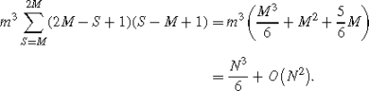
• (2) Consider i+k=j+l+N. Note 1≤k≤N requires $0\leq \eta _{2} +\eta_{4} -\eta_{1} +\frac{N}{m}\leq\frac{N}{m} \Rightarrow-\frac {N}{m}\leq\eta_{2} +\eta_{4} -\eta_{1}\leq0$. Similar to the i+k=j+l case, we write $M =\frac{N}{m}$ and S=η ₂+η ₄, and then $-\frac{N}{m}\leq S -\eta_{1}\leq0 \Rightarrow S\leq\eta_{1}\leq M+S$ where obviously S≤M. We have S+1 ways to choose (η ₂,η ₄) s.t. η ₂+η ₄=S, and M−S+1 choices of η ₁. The number of (i,j,l) is thus

  $$m^3\sum_{S=0}^M (S+1)(M-S+1) =m^3 \biggl(\frac {M^3}{6} +M^2+\frac {5}{6}M\biggr) =\frac{N^3}{6} +O\bigl(N^2\bigr).$$

  (B.2)

• (3) Consider i+k=j+l−N. Now 1≤k≤N requires $0\leq \eta _{2} +\eta_{4} -\eta_{1} -\frac{N}{m}\leq\frac{N}{m} \Rightarrow\frac {N}{m}\leq\eta_{2} +\eta_{4} -\eta_{1} \leq\frac{2N}{m}$. Again, we write $M =\frac{N}{m}$ and S=η ₁+η ₄, and then M≤S−η ₁≤2M⇒S−2M≤η ₁≤S−M where obviously S≥M. We have 2M−S+1 ways to choose (η ₂,η ₄) s.t. η ₂+η ₄=S, and S−M+1 choices of η ₁. The number of (i,j,l) is thus

  

  (B.3)

Therefore, with the additional diagonal conditions i+k=j+l+N and i+k=j+l−N induced by the circulant structure, the number of (i,j,l) is of the order $(\frac{2}{3}+\frac{1}{6}+\frac {1}{6})N^{3}=N^{3}$, i.e. the circulant structure makes up the obstructions to Diophantine equations in the Toeplitz case. Since the η _ℓ ’s do not matter for the modulo condition, to make a non-trivial configuration, we may choose three η _ℓ ’s freely, each with $\frac{N}{m}$ choices, and then choose some ϵ _ℓ ’s that satisfy the modulo condition, which we will study below.

For the modulo condition, it is necessary to figure out which zones the four entries are located in. Recall that the diagonal condition will always ensure that two paired entries are located in different areas. For the 4th moment, each of the 3 variations of the diagonal condition is sufficient to ensure that any pair of entries involved are located in the right zones. We may check this rigorously by enumerating all possibilities of the zone-wise locations of the 4 entries, e.g. if i+k=j+l+N, if a _ij ∈zone 1, then a _kl ∈zone 2.⁸ As a result, for a pair of matrix elements in the diagonal matching, say a _ij =a _kl , if i determines the slot in an m-pattern for a _ij and thus matters for the modulo condition, then l determines for a _kl ; if j determines for a _ij , then k determines for a _kl , and vice versa.

With the zone-wise issues settled, we study how to obtain a non-trivial configuration for the 4th moment. Recall the modulo condition for the diagonal matching: $i\mathcal{R}l \mbox{ or }j\mathcal{R}k$, $j\mathcal{R}i \mbox{ or }k\mathcal{R}l$. This entails 2²=4 sets of equivalence relations,

$$i\mathcal{R}l\mathcal{R}j; i\mathcal{R}l\mathcal {R}k, j\mathcal {R}k\mathcal{R}i, j\mathcal{R}k\mathcal{R}l.$$

(B.4)

Each set of equivalence relations appears with a certain probability, depending on the zone-wise locations of the 4 entries. For example, $i\mathcal{R}l\mathcal{R}j$ follows from $i\mathcal{R}l$ and $j\mathcal{R}i$, which requires both a _ij and a _jk ∈Area I. Regardless of the probability with which each set occurs, we choose one free index with N choices, and then another two indices such that these 3 indices are related to each other under $\mathcal{R}$. The number of choices of the two indices after the free one is determined solely by the number of occurrences of the elements in an m-pattern.

We give a specific example of making a non-trivial configuration for the 4th for two simple patterns {a,b,a,b} and {a,a,b,b}. Under the condition i+k=j+l, if a _ij ∈zone 1 and a _jk ∈ zone 3, then a _kl ∈zone 4 and a _li ∈zone 2. We first select η ₁,η ₂,η ₄ such that i,j,l and k=j+l−i satisfy the zone-wise locations.⁹ In this case, based on pairing conditions (B.1), pairing a _ij =a _kl and a _jk =a _li will require $\epsilon_{1}\mathcal{R}\epsilon_{4}$ and $\epsilon _{2}\mathcal{R}\epsilon_{1}$, or equivalently $\epsilon_{1}\mathcal {R}\epsilon _{2}\mathcal{R}\epsilon_{4}$. Without loss of generality, we can start with a free ϵ ₁ with 4 choices, then there are 2 free choices for each of ϵ ₂ and ϵ ₄, and then we have a non-trivial configuration. We have similar stories under the other two variations of the diagonal condition and with other zone-wise locations of a _ij and a _kl . Therefore, we can choose three out of four η _ℓ ’s freely, each with $\frac{N}{4}$ choices, then one ϵ _ℓ with 4 choices, then another two ϵ _ℓ ’s each with 2 choices, and finally the last index is determined under the diagonal condition. As discussed before, such a choice of indices will always satisfy the zone-wise requirements and thus the ϵ-based pairing conditions. Thus there are $(\frac{N}{4})^{3} \cdot4\cdot 2\cdot2 =\frac{N^{3}}{4}$ choices of (i,j,k,l) that will produce a non-trivial configuration. It follows that the contribution from the diagonal matching to the 4th moment is $\frac{1}{N^{3}}(\frac{2}{3}+\frac{1}{6}+\frac{1}{6})\frac{N^{3}}{4} =\frac{1}{4}$.

The computation of the 4th moment for the simple patterns {a,b,a,b} and {a,a,b,b} can be immediately generalized to the 4th moment for other patterns. As emphasized before, both adjacent matchings contribute fully to the 4th moment regardless of the m-pattern. For diagonal matching, the system of Diophantine equations induced by the diagonal condition are also independent of the m-pattern in question, and the way we count possible configurations can be easily generalized to an arbitrary m-pattern. We have thus proved Lemma B.1.

Note that Lemma B.1 implies that the 4th moment for any pattern depends solely on the frequency at which each element appears in an m-period. Besides the {a,a,b,b} pattern that we have studied in depth, we may easily test two extreme cases. One case where n=m, i.e. each random variable appears only once, represents the m-block circulant matrices from Theorem 1.4 for which the 4th moment is $2+\frac {1}{m^{2}}$ (and m=1 represents the circulant matrices for which the 4th moment is 3). Numerical simulations for numerous patterns including {a,a,b}, {a,b,b}, {a,b,b,a}, {a,b,c,a,b,c}, {a,b,c,d,e,e,d,c,b,a} et cetera support Lemma B.1 as well; we present results of some simulations in Tables 1, 2 and 3.

2.3 B.3 Existence and Convergence of High Moments

Although it is impractical to find every moment for a general m-block circulant pattern using brute-force computation, we are still able to prove that, for any m-block circulant pattern, every moment exists, is finite (and satisfies certain bounds), and that there exists a limiting spectral distribution. In addition, the empirical spectral measure of a typical real symmetric m-block circulant matrix converge to this limiting measure, and we have convergence in probability and almost sure convergence.

We have shown that all the odd moments vanish as N→∞, and thus we focus on the even moments. We need to prove the following theorem.

Theorem B.2

For any patterned m-block circulant matrix ensemble, lim _N→∞ M _2k (N) exists and is finite.

Proof

It is trivial that M _2k (N) is finite. As discussed before, it is bounded below by the 2kth moment for the ensemble of m-block circulant matrices where, in the m-pattern, each element is distinct, and more importantly it is bounded above by the 2kth moment for the ensemble of circulant matrices, and we know that the limiting spectral distribution for this matrix ensemble is a Gaussian.

We now show that lim _N→∞ M _2k (N) exists. To calculate M _2k (N), we match 2k elements from the matrix, $\{a_{i_{1}i_{2}},a_{i_{2}i_{3}},\ldots,a_{i_{2k}i_{1}}\}$, in k pairs, where i _ℓ ∈{1,2,…,N} and this will give (2k−1)!! matchings. For each matching, there are a certain number of configurations, and most of such configurations do not contribute to the moments as N→∞.

For the m-block circulant pattern, the equivalence relation $\mathcal {R}$ implies that $\epsilon_{s}\mathcal{R}\epsilon_{t+1}\Leftrightarrow\epsilon_{s}=\epsilon_{t+1}$, and since m|(ϵ _s −ϵ _s+1+ϵ _t −ϵ _t+1), we have ϵ _s+1=ϵ _t as well (see (B.1)).¹⁰ Thus $\eta_{s}-\eta_{s+1}+\eta_{t}-\eta _{t+1} =0\text{ or }\pm\frac{N}{m}$, three equations that have $(\frac{N}{m})^{3} +O((\frac{N}{m})^{2})$ solutions in total, as we have shown in the 4th moment computation.

However, if there are repeated elements in an m-period, then $\epsilon_{s}\mathcal{R}\epsilon_{t+1}$ no longer necessitates ϵ _s =ϵ _t+1, and it is possible that (ϵ _s −ϵ _s+1+ϵ _t −ϵ _t+1)=±m. Thus, the zone-wise locations of elements matter in making non-trivial configurations. Recall that the zone-wise location (see (B.1)) of an element $a_{i_{s}i_{s+1}}$ is determined by (i _s+1−i _s ): if $a_{i_{s}i_{s+1}}$ is in zone 1 or 3 (Area I), ϵ _s determines the slot of $a_{i_{s}i_{s+1}}$ in an m-period; if $a_{i_{s}i_{s+1}}$ is in zone 2 or 4 (Area II), ϵ _s+1 determines the slot of $a_{i_{s}i_{s+1}}$ in an m-period. In addition, the diagonal condition will always ensure that two paired entries $a_{i_{s}i_{s+1}}$ and $a_{i_{t}i_{t+1}}$ are located in different areas.

Recall that for any matching $\mathcal{M}$, the k pairs of matrix elements, each pair in the form of $a_{i_{s}i_{s+1}}=a_{i_{t}i_{t+1}}$, are fixed. For any $\mathcal{M}$, to make a non-trivial configuration, we first choose an ϵ vector of length 2k. If we choose all the ϵ _ℓ ’s freely, there are m ^2k possible choices for an ϵ vector, most of which do not meet the modulo condition, and trivially, m ^2k is an upper bound for the number of valid ϵ vectors. It is noteworthy that out of the 2k ϵ _ℓ ’s of an ϵ vector, only some of the ϵ _ℓ ’s will matter for the modulo condition. Which ϵ _ℓ ’s in fact matter depends on how we pair the 2k matrix entries $a_{i_{s}i_{s+1}}$’s and the zone-wise locations of the paired $a_{i_{s}i_{s+1}}$’s, which we cannot determine without fixing the η _ℓ ’s (and thus the i _ℓ ’s).

However, for any matching, the way we pair the 2k matrix entries into k pairs is fixed, and for each fixed pair $a_{i_{s}i_{s+1}}=a_{i_{t}i_{t+1}}$, two ϵ _ℓ ’s will matter for the modulo condition: either $\epsilon_{s}\mathcal {R}\epsilon_{t+1}$ or $\epsilon_{s+1}\mathcal{R}\epsilon_{t}$. Thus there are 2^k ways to choose k pairs of ϵ _ℓ ’s for each matching. For each way of fixing the k pairs of ϵ _ℓ ’s, we examine each ϵ pair, say $(\epsilon_{\ell_{1}},\epsilon _{\ell_{2}})$, and there are a certain number of choices of $(\epsilon_{\ell _{1}},\epsilon _{\ell_{2}})$ such that $\epsilon_{\ell_{1}}\mathcal{R}\epsilon_{\ell_{2}}$. Continuing in this way, for each ϵ pair, we choose two ϵ _ℓ ’s that satisfy the equivalence relation $\mathcal {R}$. Note that an ϵ _ℓ may matter twice, once, or never for the modulo condition depending on the zone-wise locations of the $a_{i_{s}i_{s+1}}$’s. We then choose the other ϵ _ℓ ’s that do not matter for the modulo condition such that for each pair of $a_{i_{s}i_{s+1}}=a_{i_{t}i_{t+1}}$, we have ϵ _s −ϵ _s+1+ϵ _t −ϵ _t+1=0 or ±m, and finally we have a valid ϵ vector. The number of valid ϵ vectors will be determined by m, k, and the pattern of an m-period, but will be independent of N since the system of k equivalence relations for the modulo condition does not involve N.

With a valid ϵ vector, we have fixed the zone-wise locations of the 2k matrix elements by fixing the ϵ _ℓ ’s that matter for the modulo condition. We now turn to the diagonal condition and study the η _ℓ ’s. With k equations in the form of

$$m(\eta_{s}-\eta_{s+1}+\eta_{t}-\eta _{t+1})+(\epsilon _{s}-\epsilon_{s+1}+\epsilon_{t}-\epsilon_{t+1}) =0\quad\text{or }{\pm}N,$$

(B.5)

and (ϵ _s −ϵ _s+1+ϵ _t −ϵ _t+1) known in each of the k equations, we in fact have k equations in the form of

$$\eta_{s}-\eta_{s+1}+\eta_{t}-\eta_{t+1}=\gamma,$$

(B.6)

where $\gamma\in\{0,\pm1,\frac{N}{m},\frac{N}{m}\pm1,-\frac {N}{m},-\frac{N}{m}\pm1\}$. This gives us k+1 degrees of freedom in choosing the η _ℓ ’s, and trivially, we can have at most $(\frac{N}{m})^{k+1}$ vectors of η _ℓ ’s. Since the ϵ vector is fixed, for one equation η _s −η _s+1+η _t −η _t+1=γ, there are only 3 choices of γ. With k equations in this form, we have at most 3^k systems of η equations. Note that not all of the η vectors satisfying an η equation system derived from the diagonal condition will help make a non-trivial configuration, since the η _ℓ ’s need to be chosen such that the resulted $a_{i_{s}i_{s+1}}$’s will satisfy the zone-wise locations in order to be coherent with the pre-determined ϵ vector. For example, if in a pair of matrix entries $a_{i_{s}i_{s+1}}=a_{i_{t}i_{t+1}}$ where $\epsilon_{s}\mathcal {R}\epsilon_{t+1}$, even though the η _ℓ ’s are chosen such that η _s −η _s+1+η _t −η _t+1=γ, it is possible that $a_{i_{s}i_{s+1}},a_{i_{t}i_{t+1}}$ are located in certain zones such that we need $\epsilon_{s+1}\mathcal{R}\epsilon _{t}$ to ensure a non-trivial configuration.

The following steps mirror those in [18]. Denote an η equation system by $\mathcal{S}$. For any $\mathcal{S}$ we have k equations with $\eta_{1}, \eta_{2},\ldots,\eta_{2k}\in\{1,2,\dots ,\frac{N}{m}\}$. Let $z_{\ell}=\frac{\eta_{\ell}}{N/m}\in\{\frac {m}{N},\frac{2m}{N},\ldots,1\}$. Without the zone-wise concerns discussed before, the system of k equations would have k+1 degrees of freedom and determine a nice region in the (k+1)-dimensional unit cube. Taking into account the zone-wise concerns, however, we will still have k+1 degrees of freedom. For example, for a pair of matrix elements $a_{i_{s}i_{s+1}}=a_{i_{t}i_{t+1}}$, the system $\mathcal{S}$ requires η _s −η _s+1+η _t −η _t+1=γ. If we need $\epsilon_{s}\mathcal{R}\epsilon_{t+1}$ to make a non-trivial configuration, say $a_{i_{s}i_{s+1}}\in$ zone 1, then we will obtain an additional equation $0\leq i_{s+1}-i_{s}\leq\frac{N}{2}-1\Rightarrow0\leq(\eta_{s+1}-\eta_{s})+\epsilon_{s+1}-\epsilon _{s}\leq\frac{N}{2}-1$ with (ϵ _s+1−ϵ _s )∈{−m+1,−m+2,…,0,1,…,m−2,m−1}. Based on the region determined by η _s −η _s+1+η _t −η _t+1=γ, this additional zone-related restriction will only allow a slice of the region for us to choose valid η _ℓ ’s. With k zone-wise restrictions, only a proportion of the original region in the unit cube will be preserved for the choice of the η vector. Nevertheless, the “width” of each slice is of order $\frac{N}{2}$, and we still have k+1 degrees of freedom.

Therefore, with m fixed and as N→∞, we obtain to first order the volume of this region, which is finite. Unfolding back to the η _ℓ ’s, we obtain $M_{2k}(\mathcal{S})(\frac {N}{m})^{k+1}+O_{k}((\frac{N}{m})^{k})$, where $M_{2k}(\mathcal{S})$ is the volume associated with this η system. Summing over all η systems, we obtain the number of non-trivial configurations for the 2kth moment from this particular ϵ vector. Next, within a given matching $\mathcal{M}$, we sum over all valid ϵ vectors, the number of which is independent of N as we have shown before. In the end, we sum over the (2k−1)!! matchings to obtain M _2k N ^k+1+O _k (N ^k), and the 2kth moment is simply $\frac {M_{2k}N^{k+1}+O_{k}(N^{k})}{N^{k+1}}=M_{2k}+O(\frac{1}{N})$. □

The above proves the existence of the moments. The convergence proof follows with only minor changes to the convergence proofs from [18, 29].

References

Abramowitz, M., Stegun, I.A.: Handbook of Mathematical Functions. Dover, New York (1965). Online at http://people.math.sfu.ca/~cbm/aands/
Baik, J., Borodin, A., Deift, P., Suidan, T.: A model for the bus system in Cuernevaca (Mexico). Math. Phys. (2005), 1–9. Online available at http://arxiv.org/abs/math/0510414
Basak, A., Bose, A.: Limiting spectral distribution of some band matrices. Periodica Math. Hungarica 63(1), 113–150 (2011)
Basak, A., Bose, A.: Balanced random Toeplitz and Hankel matrices. Electron. Comm. Probab. 15, 134–148
Banerjee, S., Bose, A.: Noncrossing partitions, Catalan words and the semicircle law. J. Theor. Probab. doi:10.1007/s10959-011-0365-4
Beckwith, O., Miller, S.J., Shen, K.: Distribution of eigenvalues of weighted, structured matrix ensembles, preprint
Bose, A., Chatterjee, S., Gangopadhyay, S.: Limiting spectral distributions of large dimensional random matrices. J. Indian Stat. Assoc. 41, 221–259 (2003)
Bose, A., Hazra, R.S., Saha, K.: Patterned random matrices and notions of independence, Technical Report R3/2010 (2010), Stat-Math Unit, Kolkata. Available online at http://www.isical.ac.in/~statmath
Bose, A., Mitra, J.: Limiting spectral distribution of a special circulant. Stat. Probab. Lett. 60(1), 111–120 (2002)
Bryc, W., Dembo, A., Jiang, T.: Spectral measure of large random Hankel, Markov, and Toeplitz matrices. Ann. Probab. 34(1), 1–38 (2006)
Dyson, F.: Statistical theory of the energy levels of complex systems: I, II, III. J. Math. Phys. 3, 140–156 (1962), 157–165, 166–175
Dyson, F.: The threefold way. Algebraic structure of symmetry groups and ensembles in quantum mechanics. J. Math. Phys. 3, 1199–1215 (1962)
Erdős, L., Ramirez, J.A., Schlein, B., Yau, H.-T.: Bulk Universality for Wigner Matrices, preprint. http://arxiv.org/abs/0905.4176
Erdős, L., Schlein, B., Yau, H.-T.: Wegner estimate and level repulsion for Wigner random matrices, preprint. http://arxiv.org/abs/0905.4176
Firk, F.W.K., Miller, S.J.: Nuclei, primes and the random matrix connection. Symmetry 1, 64–105 (2009). doi:10.3390/sym1010064
Forrester, P.J.: Log-Gases and Random Matrices. London Mathematical Society Monographs, vol. 34. Princeton University Press, Princeton (2010)
Gradshteyn, I., Ryzhik, I.: Tables of Integrals, Series, and Products. Academic Press, New York (1965)
Hammond, C., Miller, S.J.: Eigenvalue spacing distribution for the ensemble of real symmetric Toeplitz matrices. J. Theor. Probab. 18(3), 537–566 (2005)
Harer, J., Zagier, D.: The Euler characteristic of the moduli space of curves. Invent. Math. 85, 457–485 (1986)
Hatcher, A.: Algebraic Topology. Cambridge University Press, Cambridge (2002)
Hayes, B.: The spectrum of Riemannium. Am. Sci. 91(4), 296–300 (2003)
Jackson, S., Miller, S.J., Pham, V.: Distribution of eigenvalues of highly palindromic Toeplitz matrices. http://arxiv.org/abs/1003.2010
Jakobson, D., Miller, S.D., Rivin, I., Rudnick, Z.: Eigenvalue spacings for regular graphs. In: Emerging Applications of Number Theory, Minneapolis, 1996. The IMA Volumes in Mathematics and its Applications, vol. 109, pp. 317–327. Springer, New York (1999)
Kargin, V.: Spectrum of random Toeplitz matrices with band structure. Electron. Commun. Probab. 14, 412–421 (2009)
Kopp, G.S., Koloğlu, M., Miller, S.J., Strauch, F., Xiong, W.: The limiting spectral measure for ensembles of symmetric block circulant matrices. arXiv version. http://arxiv.org/abs/1008.4812
Krbalek, M., Seba, P.: The statistical properties of the city transport in Cuernavaca (Mexico) and Random matrix ensembles. J. Phys. A, Math. Gen. 33, L229–L234 (2000)
Ledoux, M.: A recursion formula for the moments of the Gaussian orthogonal ensemble. Ann. IHP 45(3), 754–769 (2009)
Liu, D.-Z., Wang, Z.-D.: Limit distribution of eigenvalues for random Hankel and Toeplitz band matrices, to appear in J Theor Probab. http://arxiv.org/abs/0904.2958
Massey, A., Miller, S.J., Sinsheimer, J.: Distribution of eigenvalues of real symmetric palindromic Toeplitz matrices and circulant matrices. J. Theor. Probab. 20(3), 637–662 (2007)
Meckes, M.: The spectra of random abelian G-circulant matrices, preprint. http://arxiv.org/PS_cache/arxiv/pdf/1109/1109.5675v1.pdf
Miller, S.J., Novikoff, T., Sabelli, A.: The distribution of the second largest eigenvalue in families of random regular graphs. Exp. Math. 17(2), 231–244 (2008)
McKay, B.: The expected eigenvalue distribution of a large regular graph. Linear Algebra Appl. 40, 203–216 (1981)
Montgomery, H.: The pair correlation of zeros of the zeta function. In: Analytic Number Theory. Proceedings of Symposia in Pure Mathematics, vol. 24, pp. 181–193. AMS, Providence (1973)
Stein, E., Shakarchi, R.: Fourier Analysis: An Introduction. Princeton University Press, Princeton (2003)
Stein, E., Shakarchi, R.: Complex Analysis. Princeton University Press, Princeton (2003)
Takacs, L.: A moment convergence theorem. Am. Math. Mon. 98(8), 742–746 (1991)
Tao, T., Vu, V.: From the Littlewood–Offord problem to the circular law: Universality of the spectral distribution of random matrices. Bull. Am. Math. Soc. 46, 377–396 (2009)
Tao, T., Vu, V.: Random matrices: Universality of local eigenvalue statistics up to the edge, preprint. http://arxiv.org/PS_cache/arxiv/pdf/0908/0908.1982v1.pdf
Wigner, E.: On the statistical distribution of the widths and spacings of nuclear resonance levels. Proc. Camb. Philol. Soc. 47, 790–798 (1951)
Wigner, E.: Characteristic vectors of bordered matrices with infinite dimensions. Ann. Math. 2(62), 548–564 (1955)
Wigner, E.: Statistical properties of real symmetric matrices. In: Canadian Mathematical Congress Proceedings, pp. 174–184. University of Toronto Press, Toronto (1957)
Wigner, E.: Characteristic vectors of bordered matrices with infinite dimensions. II. Ann. Math. Ser. 2 65, 203–207 (1957)
Wigner, E.: On the distribution of the roots of certain symmetric matrices. Ann. Math. Ser. 2 67, 325–327 (1958)
Wishart, J.: The generalized product moment distribution in samples from a normal multivariate population. Biometrika A 20, 32–52 (1928)
Xiong, W.: The limiting spectral measure for the ensemble of generalized real symmetric period m-circulant matrices, senior thesis (advisor S.J. Miller), Williams College (2011)
Zvonkin, A.: Matrix integrals and map enumeration: An accessible introduction. Math. Comput. Model. 26(8–10), 281–304 (1997)
Acknowledgements
M. Koloğlu and G.S. Kopp were partially supported by Williams College and NSF Grants DMS0855257 and DMS0850577, and S.J. Miller was partly supported by NSF Grant DMS0970067. It is a pleasure to thank our colleagues from the Williams College 2010 SMALL REU program as well as the participants of the ICM Satellite Meeting in Probability & Stochastic Processes (Bangalore, 2010) for many helpful conversations, especially Arup Bose and Rajat Hazra. We would also like to thank Elizabeth Townsend Beazley for comments on Wentao Xiong’s senior thesis, which is the basis of Appendix B.
Author information
Authors and Affiliations
Corresponding author