Iterative Grossone-Based Computation of Negative Curvature Directions in Large-Scale Optimization

Abstract

We consider an iterative computation of negative curvature directions, in large-scale unconstrained optimization frameworks, needed for ensuring the convergence toward stationary points which satisfy second-order necessary optimality conditions. We show that to the latter purpose, we can fruitfully couple the conjugate gradient (CG) method with a recently introduced approach involving the use of the numeral called Grossone. In particular, recalling that in principle the CG method is well posed only when solving positive definite linear systems, our proposal exploits the use of grossone to enhance the performance of the CG, allowing the computation of negative curvature directions in the indefinite case, too. Our overall method could be used to significantly generalize the theory in state-of-the-art literature. Moreover, it straightforwardly allows the solution of Newton’s equation in optimization frameworks, even in nonconvex problems. We remark that our iterative procedure to compute a negative curvature direction does not require the storage of any matrix, simply needing to store a couple of vectors. This definitely represents an advance with respect to current results in the literature.

1 Introduction

We consider the solution of the nonconvex unconstrained optimization problem $\min _{x \in \mathbb {R}^n} f(x)$, where $f: \mathbb {R}^n \rightarrow \mathbb {R}$ is a nonlinear smooth function and n is large. Despite the use of the term ‘minimization’ in the last problem, most of the methods proposed in the literature (for its solution) generate a sequence of points $\{x_k\}$, which is only guaranteed to converge to stationary points. Thus, specific methods need to be applied in case stationary points for the above problem, satisfying also second-order necessary optimality conditions, are sought (see, for instance, the seminal papers [1,2,3,4,5,6,7] in the framework of truncated Newton methods). Observe that additional care when using the latter methods is definitely mandatory, since imposing standard first-order stationarity conditions may not in general ensure convexity of the quadratic model of the objective function, in a neighborhood of the solution points. In this regard, the computation of so-called negative curvature directions for the objective function is an essential tool (see also the recent papers [4, 8]), to guarantee convergence to stationary points which satisfy second-order necessary conditions.

Here, we want to provide a framework for the computation of negative curvature directions of quadratic functions, to be used within globally convergent iterative methods for large-scale nonlinear programming. Observe that the asymptotic convergence of iterative methods, toward second-order stationary points, implies that the Hessian matrix at limit points must be positive semidefinite. This fact requires that in principle the iterative methods adopted must be able to fully explore the eigenspaces of the Hessian matrix, at the current iterate, at least in a neighborhood of the stationary points. Equivalently, the optimization method adopted will have to efficiently cope also with nonconvexities of the objective function. The latter fact issues specific concerns in case n is large, since the computational effort to solve a nonlinear programming problem can be strongly affected by the scale.

In particular, as shown in [3, 5, 9], exploiting the nonconvexities of f(x) can be accomplished by suitable Newton–Krylov methods (in the context of Hessian-free truncated Newton methods), such that at each outer iteration j, a pair of search directions $(s_j, d_j)$ is computed, satisfying specific properties. Namely, the vector $s_j$ must be a direction which approximately solves Newton’s equation $\nabla ^2 f (x_j)~s=-\nabla f(x_j)$ at $x_j$. Its purpose is essentially that of ensuring the efficient convergence of the sequence $\{x_j\}$ to stationary points. On the other hand, the nonascent direction $d_j$ is a negative curvature direction (if any) for the objective function at $x_j$. That is, $d_j$ is a nonascent direction such that $d_j^T \nabla ^2 f (x_j) d_j \le 0$, satisfying suited conditions in order to force convergence to those stationary points where second-order necessary optimality conditions hold. In particular, $d_j$ should resemble an eigenvector corresponding to the least negative eigenvalue of the Hessian matrix $\nabla ^2 f(x_j)$. In [3, 5] the direction $d_j$ is obtained as by-product of the Krylov-subspace method applied for solving Newton’s equation, though an expensive storage is required in [5] and a heavy computational burden is necessary in the approach proposed in [3].

To overcome these drawbacks, in [9] an important novelty is introduced, namely the iterative computation of the sequence $\{d_j\}$, not requiring neither expensive computations nor excessive storage. This novel approach is based on the use of the so-called Planar-CG method which is a modification of the conjugate gradient method in [11]. In particular, in [9], at any iterate $x_j \in \mathbb {R}^n$, the vector $d_j$ is computed through the linear combination of a few n-real vectors, generated by the used Krylov subspace method. It was proved that on nonconvex problems, the overall exact computation of $d_j$ simply requires at iterate $x_j$ the storage of at most four n-real vectors. Even if this approach revealed effective, it presents some drawbacks related to a cumbersome analysis.

In this paper, partially starting from the drawbacks of the proposal in [9], we aim at describing a strong simplification in the computation of the directions $\{d_j\}$, by using a novel approach which extends some ideas in [12]. Namely, we adopt the Krylov-based method defined in [12], being the symbol for the grossone (see [13]), in order to generate a suitable matrix factorization which allows the computation of $\{d_j\}$. Similarly to [12], we first show that the CG is an ideal candidate to generate the latter matrix factorization. However, it may reveal serious disadvantages on nonconvex problems. In this regard, represents a natural generalization of the CG, and with some care allows to extend CG properties on indefinite problems. Then, the is used to generate directions in eigenspaces of the Hessian matrix associated with negative eigenvalues and to provide a suitable matrix factorization, which allows to exploit the results in [14].

We also propose a numerical experience, where we assess the effectiveness of the negative curvature directions computed in the current paper. We prefer to skip a numerical comparison between our proposal and those in [3, 5, 10], the latter requiring an expensive matrix storage or the need for recomputing some quantities/vectors. This risks to make the comparison unfair, inasmuch as in [9] and here we prove that an inexpensive iterative computation of $d_j$ is obtained, by storing at most two (four in [9]) working vectors.

To sum up, considering [9] as a reference paper with respect to our analysis, the main enhancements of the approach in the current paper can be summarized as follows:

• in [9] the computation of the negative curvature direction $d_j$, at iterate $x_j$, requires the storage of up to four vectors, while here we propose a method requiring the storage of only two vectors;

• the theory in [9] heavily relies on complicate matrix factorizations, due to the structure of the Planar-CG method therein adopted. Conversely, here the analysis through grossone only indirectly uses matrix factorizations provided by a Planar-CG method. Moreover, the Planar-CG method indirectly adopted here is definitely simpler that the one adopted in [9]. Hence, here the theoretical analysis to prove convergence of the sequence $\{x_j\}$ to stationary points, satisfying second-order conditions, is drastically simplified;

• the strategy adopted in [9] to compute the search directions is definitely more computationally expensive than the one proposed here;

• as regards numerical results, we do not claim that our proposal is always more efficient than the one in [9], depending on the problem in hand.

The paper is organized as follows: Sect. 2 reports some preliminaries on the use of negative curvature directions within truncated Newton methods. In Sect. 3, we give some basics on grossone, in order to motivate its use within the algorithm . Section 4 emphasizes the importance of certain matrix factorizations, in order to iteratively compute the final negative curvature direction. Section 5 stresses the importance of pairing with the approach in [14]. Moreover, the last section explicitly yields our formula for determining the negative curvature direction. Finally, Sect. 6 contains a numerical experience on our proposal, and Sect. 7 reports some conclusions and future research perspectives.

In this paper, we use standard notations for vectors and matrices. With $\Vert \cdot \Vert$, we indicate the Euclidean norm. $\lambda [A]$ is a general eigenvalue of matrix $A \in \mathbb {R}^{n \times n}$, and $A\succ 0 ~ [A\succeq 0]$ indicates that A is positive definite [semidefinite]. $e_k \in \mathbb {R}^n$ represents the kth unit vector, while the symbol represents the numeral grossone (see also [13]).

2 Negative Curvature Directions in Truncated Newton Methods

Hereafter, we will use the following scheme

$$\begin{aligned} \min _{x \in \mathbb {R}^n} f(x), \end{aligned}$$

(1)

with $f \in C^2(\mathbb {R}^n)$, as a general reference for an unconstrained optimization problem. Moreover, the equation

$$\begin{aligned} \nabla ^2 f (x_j)~s=-\nabla f(x_j) \end{aligned}$$

(2)

represents Newton’s equation associated with problem (1).

The use of negative curvature directions in the framework of truncated Newton methods was introduced in the early papers [6, 7], in order to define algorithms converging toward second-order critical points, namely stationary points where the Hessian matrix is positive semidefinite. Following the approach in [7], the sequence of negative curvature directions $\{d_j\}$ is expected to satisfy the conditions in the next assumption.

Assumption 2.1

Given problem (1), with $f \in C^2(\mathbb {R}^n)$, the nonascent directions in the sequence $\{d_j\}$ are bounded and satisfy the conditions

• (a) $\nabla f (x_j)^T d_j \le 0, \quad d_j^T H_j d_j \le 0$,

• (b) if $\ \lim _{j \rightarrow \infty } d_j^T \nabla ^2 f(x_j) d_j = 0 \$ then $\ \lim _{j \rightarrow \infty } \min \left\{ 0, ~\lambda _{\mathrm {\tiny min}}\left[ \nabla ^2 f(x_j)\right] \right\} = 0,$

where $\lambda _{\mathrm {\tiny min}}\left[ \nabla ^2 f(x_j) \right]$ is the smallest eigenvalue of the Hessian matrix $\nabla ^2 f(x_j)$.

The approach adopted in [7] may be generalized to some extent (see, for instance, the proposal in [5]), by suitably weakening conditions the directions $\{d_j\}$ are subject to.

Roughly speaking, the condition (a) in Assumption 2.1 implies that at any iterate $x_j$, the nonascent vector $d_j$ must be a nonpositive curvature direction. Moreover, as in condition (b), when the quantity $d_j^T \nabla ^2 f (x_j) d_j$ approaches zero, then the sequence $\{x_j\}$ is approaching a region of convexity for the function f(x). Indeed, in such a case there will be no more chances to compute a negative curvature direction satisfying $d_j^T \nabla ^2 f (x_j) d_j < 0$, so that eventually the condition $d_j^T \nabla ^2 f (x_j) d_j \rightarrow 0$ must hold. Of course, on convex problems, negative curvature directions are not present, so that points provided by Newton–Krylov methods eventually satisfy also second-order stationarity conditions.

We recall that the main purpose of Newton–Krylov methods is to compute the (possibly) infinite sequence $\{x_j\}$, such that at least one of its subsequences is convergent to a stationary point of f(x). In this regard, Assumption 2.1 does not imply a unique choice of $d_j$ at iteration j. In fact, in order to fulfill (b) of Assumption 2.1, it suffices to compute $d_j$ so that $d_j^T \nabla ^2 f (x_j) d_j \le v_j^T \nabla ^2 f (x_j) v_j$, being $v_j$ an eigenvector associated with the smallest eigenvalue of $\nabla ^2 f (x_j)$. In addition, $d_j$ becomes essential only eventually; i.e., far from a stationary point, it might be unnecessary to force convergence toward regions of convexity for f(x). Nevertheless, using information associated with the negative curvature direction $d_j$, also when far from a solution point, may considerably enhance efficiency. The latter fact was evidenced, for instance, in [3, 5, 10] and intuitively follows from the next reasoning. Given the local quadratic expansion

$$\begin{aligned} q_j(d) = f(x_j)+ \nabla f(x_j)^Td+ \frac{1}{2} d^T \nabla ^2f(x_j) d, \end{aligned}$$

at $x_j$, the directional derivative of $q_j(d)$

$$\begin{aligned} \nabla q_j(d)^Td = \nabla f(x_j)^T d + d^T \nabla ^2f(x_j) d, \end{aligned}$$

along d, may strongly decrease when d is not only a descent vector, but also a negative curvature direction. This fact is explicitly used in [2, 3, 5, 10] when a negative curvature direction $d_j$ is adopted, at any iteration j, even if it is possibly not associated with an eigenvector z corresponding to the smallest negative eigenvalue of $\nabla ^2f(x_j)$.

Further developments on the computation of negative directions, to be used within truncated Newton methods, have been introduced in the already mentioned papers [3, 5, 9]. In particular, in [3, 5] the direction $d_j$ is obtained as by-product, when applying a Krylov-subspace method to solve Newton’s equation (2). However, since the Krylov method may perform, at iteration j, a number k of steps considerably smaller than n, not all the eigenspaces associated with the Hessian matrix $\nabla ^2f(x_j)$ will be explored, vanishing the search of z. Hence, only an approximation of z may be available after k steps of the Krylov-based method.

In [9], the iterative computation of the directions $\{d_j\}$ is proposed. The innovative contribution in [9] consisted of explicitly providing the iterative computation of the sequence $\{d_j\}$, without requiring burdensome re-computing (as in [3]) or any expensive storage (as in [5]). In particular, the Krylov-based procedure adopted in [9] to compute $d_j$ involves the use of the Planar-CG method, which represents an extension of the CG to nonconvex quadratic functions, where the Hessian matrix is possibly indefinite. The approach using this Planar-CG method surely proved to be effective, but it has a major disadvantage, requiring a fairly complex analysis which involves considering different and articulated subcases.

3 A Brief Introduction to the -Based Computational Methodology

The numeral

called grossone has been introduced (see a recent survey [13]) as a basic element of a powerful numeral system, allowing one to express not only finite but also infinite and infinitesimal quantities. (Analogously, the numeral 1 is a basic element allowing one to express finite quantities.) From the foundational point of view, grossone has been introduced as an infinite unit of measure equal to the number of elements of the set $\mathbb {N}$ of natural numbers. (Notice that the noncontradictoriness of the -based computational methodology has been studied in depth in [15,16,17].) From the practical point of view, this methodology has given rise both to a new supercomputer patented in several countries (see [18]) and called Infinity Computer and to a variety of applications starting from optimization (see [12, 19,20,21,22,23,24]) and going through infinite series (see [13, 25,26,27,28]), fractals and cellular automata (see [25, 29,30,31,32]), hyperbolic geometry and percolation (see [33, 34]), the first Hilbert problem and Turing machines (see [13, 35, 36]), infinite decision making processes and probability (see [13, 37,38,39]), numerical differentiation and ordinary differential equations (see [40,41,42,43]), etc.

This methodology does not contradict traditional views on infinity and infinitesimals (Cantor, Leibnitz, Robinson, etc.) and proposes just another, more computationally oriented, way to deal with these objects. In particular, in order to avoid misunderstanding it should be stressed that there exist several differences (see [44] for a detailed discussion) that distinguish the numerical

-based methodology from symbolically oriented nonstandard analysis of Robinson. Another important preliminary remark is that symbols traditionally used to work with infinities and infinitesimals ($\infty$ introduced by Wallis, Cantor’s $\omega$, $\aleph _0, \aleph _1, ...$, etc.) are not used together with

. Similarly, when the positional numeral system and the numeral 0 expressing zero had been introduced, symbols V, X and other symbols from the Roman numeral system had not been used in the positional numeral system.

The numeral

allows one to construct different numerals involving infinite, finite, and infinitesimal parts and to execute numerical computations with all of them in a unique computational framework. As a result, it becomes possible to execute arithmetical operations with a variety of different infinities and infinitesimals. As a remarkable result, indeterminate forms such as $\infty - \infty$ or $\infty \cdot 0$ are not present when one works with numbers expressed in the

-based numeral system. Traditionally existing kinds of divergences do not appear, as well. They are substituted by expressions that can contain also finite, infinite and infinitesimal parts.

In order to give some examples of arithmetical operations that can be executed in the

-based numeral system, let us consider the following numbers: and (that are examples of infinities), along with and (that are examples of infinitesimals). Then, we can compute, for instance, the following expressions:

(3)

In general, in the

-based numeral system the simplest infinitesimal numbers are represented by numerals having only negative finite powers of

(e.g., , see also examples above). The simplest infinite numbers are represented by numerals having at least one positive power of

. Then, it can be seen in (3) that ; therefore, a finite number a can be represented in the new numeral system simply as , where the numeral a itself can be written down by any convenient numeral system used to express finite numbers. These numbers are called purely finite because they do not contain infinitesimal parts. For instance, number 5 is purely finite and is finite but not purely finite, because it contains the infinitesimal part . Notice that all infinitesimals are not equal to zero. In particular, because it is a result of division of two positive numbers.

4 The Matrix Factorizations We Need

In the current and the next section, we describe how to use some Krylov-subspace methods, in order to gain advantage of a suitable factorization for the (possibly) indefinite Hessian matrix $\nabla ^2f(x_j)$. We strongly remark that we never explicitly compute here any Hessian decomposition, since our final achievements definitely rely on implicit decompositions, induced by Krylov-based methods.

As a general result, we highlight that computing negative curvature directions for f(x) at $x_j$, which match the requirements in Assumption 2.1, may reduce to a simple task when suitable factorizations of $\nabla ^2 f(x_j)$ are available. To give an intuition of the latter fact, suppose both the relations

$$\begin{aligned} M_j^T \nabla ^2 f(x_j) M_j = C_j, \qquad C_j = Q_j B_j Q_j^T, \end{aligned}$$

(4)

are available at iterate $x_j$, being $M_j \in \mathbb {R}^{n \times k}$, where $C_j, Q_j, B_j \in \mathbb {R}^{k \times k}$ are nonsingular. In this regard, the CG (Table 1) is an example of a Krylov-based method, satisfying the following properties:

Table 1 A practical implementation of the CG algorithm for the symmetric positive definite linear system $Ax = b$, with $A \in \mathbb {R}^{n \times n}$

• it provides the decompositions in (4) (see also (6)) when $\nabla ^2 f(x_j) \succ 0$, with $j \ge 1$;

• the matrices $M_j, C_j,Q_j,B_j$ have a special structure, inasmuch as (see also [45]): The columns of $M_j$ are unit orthogonal vectors, $C_j$ is tridiagonal, $Q_j$ is unit lower bidiagonal, and $B_j$ is diagonal.

Note that the Lanczos process, which represents another renowned Krylov-based method in the literature, iteratively provides the left decomposition in (4), with $C_j$ tridiagonal, but not the right one. It is indeed necessary to couple the Lanczos process with a suitable factorization of $C_j$, in order to obtain usable negative curvature directions or solvers for Newton’s equation (see, e.g., SYMMLQ/MINRES [46], SYMMBK [47]).

Now, given (4) suppose the vector $w \in \mathbb {R}^k$ is an eigenvector of $B_j$, associated with its negative eigenvalue$\lambda$, whose computation is ‘relatively simple.’ Moreover, suppose the vector $y \in \mathbb {R}^k$ is easily available, such that $Q_j^Ty=w$. Then, by (4) the equalities/inequalities

$$\begin{aligned} (M_j y)^T \nabla ^2 f(x_j) (M_j y)= & {} y^T \left[ M_j^T \nabla ^2 f(x_j) M_j \right] y \\= & {} y^TC_j y \ = \ (Q_j^T y)^T B_j (Q_j^T y) \\= & {} w^T B_j w \ = \ \lambda \Vert w \Vert ^2 \ < \ 0 \end{aligned}$$

immediately show that the direction $d_j = M_j y$ is of negative curvature for f(x) at $x_j$. In particular, thanks to the chain of equalities above, if $\lambda$ is the smallest negative eigenvalue of $B_j$, then $M_j y$ is also an eigenvector of $\nabla ^2 f(x_j)$, associated with the smallest eigenvalue of $\nabla ^2 f(x_j)$. The most renowned Krylov-subspace methods for symmetric linear systems (i.e., SYMMLQ, SYMMBK, CG, Planar-CG methods [48,49,50]) can all provide the factorizations (4) when applied to solve Newton’s equation at the iterate $x_j$. Hence, generating a negative curvature which satisfies (a) in Assumption 2.1, may not be a difficult goal. However, fulfilling also (b) and the boundedness of the latter negative curvature direction, is a less trivial task. Indeed, the counterexample in Sect. 4 of [7] issues such a drawback, when a modified Cholesky factorization of the Hessian matrix is possibly adopted.

We strongly remark this point, since our main effort here is that of coupling a Krylov-subspace method with the novel tool in the literature given by grossone. In particular, we want to show that by the use of a subset of properties which hold for grossone, we can yield an implicit matrix factorization as in (4), fulfilling also (b) and the boundedness of the final negative curvature direction $d_j$ in Assumption 2.1.

On this purpose, let us first state a general formal result for Krylov-subspace methods, which possibly summarizes the above considerations. The proof of the next lemma easily follows from Lemma 4.3 in [7] and Theorem 3.2 in [9].

Lemma 4.1

Let problem (1) be given with $f \in C^2(\mathbb {R}^n)$, and consider an iterative method for solving (1), which generates the sequence $\{x_j\}$. Let the level set ${{\mathcal {L}}}_0 = \{x \in \mathbb {R}^n \ : \ f(x) \le f(x_0)\}$ be compact, being any limit point ${\bar{x}}$ of $\{x_j\}$ a stationary point for (1), with $\left| \lambda {[\nabla ^2f({\bar{x}})]} \right|> {\bar{\lambda }} > 0$. Suppose n iterations of a Newton–Krylov method are performed to solve Newton’s equation (2) at iterate $x_j$, for a given $j \ge 0$, so that the decompositions

$$\begin{aligned} R_j^T\nabla ^2 f(x_j)R_j = T_j, \qquad T_j = L_j B_j L_j^T \end{aligned}$$

(5)

are available. Moreover, suppose $R_j \in \mathbb {R}^{n \times n}$ is orthogonal, $T_j \in \mathbb {R}^{n \times n}$ has the same eigenvalues of $\nabla ^2 f(x_j)$, with at least one negative eigenvalue, and $L_j, B_j \in \mathbb {R}^{n \times n}$ are nonsingular. Let z be the unit eigenvector corresponding to the smallest eigenvalue of $B_j$, and let ${\bar{y}} \in \mathbb {R}^n$ be the (bounded) solution of the linear system $L_j^T y = z$. Then, the vector $d_j = R_j {\bar{y}}$ is bounded and satisfies Assumption 2.1.

The vector $d_j$ computed in Lemma 4.1 may be used to guarantee the satisfaction of Assumption 2.1, i.e., the sequence $\{d_j\}$ can guarantee convergence to second-order critical points. However, three main drawbacks of the approach in Lemma 4.1 are that

$(\alpha )$:

the eigenvector z of $B_j$ and the solution of the linear system $L_j^T y = z$ should be of easy computation;

$(\beta )$:

the corresponding vector ${\bar{y}}$ should be provably bounded;

$(\gamma )$:

at iterate j the Newton–Krylov method adopted to solve (2) possibly does not perform n iterations.

Observe that according to the requirements in Assumption 2.1, after a careful consideration, the issue at item $(\gamma )$ is not really so relevant. Indeed, in any case (see also [9]) when $j \rightarrow \infty$ the convergence of the Newton–Krylov method imposes that it eventually performs n iterations [51]. On the other hand, in case at iterate $x_j$, for a finite j, $\nabla ^2f(x_j) \succeq 0$ or a vector $v \in \mathbb {R}^n$ such that $v^T \nabla ^2f(x_j)v < 0$ is unavailable, then the factorization (5) yet exists and we can simply set $d_j=0$, which satisfies (a) in Assumption 2.1 along with the boundedness requirement.

Though the CG is not well posed when $\nabla ^2 f(x_j) \not \succ 0$, in [9] the authors reported that, in case n CG steps are performed without stopping when solving Newton’s equation, the above items $(\alpha )$ and $(\beta )$ can be relatively easily fulfilled, even in case $\nabla ^2 f(x_j)$ is indefinite. In particular, these results are obtained exploiting the factorizations in Lemma 4.1, for which the CG specifically yields (Table 1)

$$\begin{aligned} R_j= & {} \left( \frac{r_1}{\Vert r_1\Vert } \ \cdots \ \frac{r_n}{\Vert r_n\Vert } \right) ,\nonumber \\ B_j= & {} \left( \begin{array}{cccc} \frac{1}{a_1} &{} &{} &{} 0 \\ &{} \ddots &{} &{} \\ &{} &{} \ \ \ddots &{} \\ 0 &{} &{} &{} \frac{1}{a_n} \end{array} \right) , ~~~ L_j = \left( \begin{array}{cccccc} 1 &{} &{} &{} &{} &{} \\ &{} &{} &{} &{} &{} \\ -\sqrt{\beta _1} &{} 1 &{} &{} &{} 0 &{} \\ &{} \ddots &{} \ddots &{} &{} &{} \\ &{} &{} \ \ \ddots &{} \ \ \ddots &{} &{} \\ &{} &{} &{} \,\,-\sqrt{\beta _{n-2}} &{} 1 &{} \\ 0 &{} &{} &{} &{} &{} \\ &{} &{} &{} &{} \,\, -\sqrt{\beta _{n-1}} &{} \ \ \ 1 \end{array} \right) .\nonumber \\ \end{aligned}$$

(6)

Thanks to the above expressions of $R_j$, $B_j$ and $L_j$, in [9] the authors proved that after n steps the CG straightforwardly yields also the bounded negative curvature direction

$$\begin{aligned} d_j = \frac{p_m}{\Vert r_m\Vert }, \end{aligned}$$

(7)

being $1 \le m \le n$ an index such that

$$\begin{aligned} \frac{1}{a_m} = \min _{i} \left\{ \frac{1}{a_i} \right\} , \end{aligned}$$

i.e.,

$$\begin{aligned} d_j = \frac{p_m}{\Vert r_m\Vert } \in \mathrm{argmin}_i \left\{ \left( \frac{p_i}{\Vert r_i\Vert } \right) ^T A \left( \frac{p_i}{\Vert r_i\Vert } \right) \right\} . \end{aligned}$$

Moreover, $d_j$ in (7) satisfies Lemma 4.1, thanks to the fact that $B_j$ is diagonal (i.e., its eigenvectors coincide with the canonical basis), $L_j$ is unit lower bidiagonal (so that the solution of $L_j^Ty=e_m$ is straightforwardly available by backtracking) and $d_j$ is provably bounded.

Our goal is that of possibly replicating an analogous reasoning, with other Krylov-based methods for indefinite linear systems, following similar guidelines. In this regard, observe that both the tasks $(\alpha )$ and $(\beta )$ might be hardly guaranteed only using, for instance, the instruments in [14], essentially because comparing with the CG, the structure of the matrices $L_j$ and $B_j$ generated by the Planar-CG method in [14] is more cumbersome. Nevertheless, in the next sections, starting from the structure of matrices $L_j$ and $B_j$, as computed by the algorithm in [14], we will show how to use in [12] in order to fulfill the hypotheses of Lemma 4.1.

5 Our Proposal: Preliminaries

To fill the gap outlined in the previous section, and recalling that in Lemma 4.1 we focus on the case where $j \rightarrow +\infty$, let us set for the sake of simplicity $A = \nabla ^2f(x_j)$, $b = -\nabla f(x_j).$ This allows us to drop the dependency on the subscript j. Consider the method in [12] (which is also reported in Table 2, for the sake of completeness. Observe that the practical implementation of Step k in currently allows the test $p_k^TAp_k \ne 0$ to be replaced by the inequality $|p_k^TAp_k| \ge \eta \Vert p_k\Vert ^2$, with $\eta >0$ small).

Table 2 The algorithm for solving the symmetric indefinite linear system $Ax = b$, $A \in \mathbb {R}^{n \times n}$. In a practical implementation of Step k of , the test $p_k^TAp_k \ne 0$ may be replaced by the inequality $|p_k^TAp_k| \ge \eta \Vert p_k\Vert ^2$, with $\eta >0$ small

The substantially coincides with the CG, as long as $p_k^TAp_k \ne 0$. Moreover, in case at Step k we have $p_k^TAp_k=0$, from Section 5.1 of [12] the generates both the vectors $r_{k+1}$ and $p_{k+1}$, such that they depend on . Furthermore, we have (after a simple computation, and using the standard Landau–Lifsits notation $O(\cdot )$)

(8)

Recalling that by definition , i.e., , then neglecting in $\alpha _{k+1}$ the terms containing negative powers of (corresponding indeed to infinitesimals with respect to the value —see Sect. 3) we have

(9)

This immediately implies that

$$\begin{aligned} \alpha _k \cdot \alpha _{k+1} < 0. \end{aligned}$$

(10)

Note that by using , similarly to the CG to solve (2), we can recover the structure of $B_j$ and $L_j$ in (6), so that (7) formally applies. However, since is infinitesimal in (9), after some computation we have (see also Sect. 5.1 of [12])

Then, in case $m=k+1$ in (7), to compute the direction $d_j$ we would have

(11)

which implies that $\Vert d_j\Vert$ is not bounded (being ) and Lemma 4.1 cannot be fulfilled. This consideration should not be surprising. Indeed, it basically summarizes the fact that similarly to the CG, is unable to provide the diagonal matrix (6) with finite entries, in case the tridiagonal matrix $T_j$ in (5) is indefinite.

Nevertheless, to overcome the latter limitation, now we show how to properly couple with the Planar-CG method in [14], in order to obtain a suitable bounded negative curvature direction which fulfills Lemma 4.1.

5.1 Coupling with the Algorithm in [14]

Following the taxonomy in Sect. 4, assume without loss of generality that the Krylov-subspace method detailed in [14] is applied to solve Newton’s equation

$$\begin{aligned} Au=b, \end{aligned}$$

(12)

and n steps are performed.¹ Again this allows us to drop the dependency on the subscript j. After some computation, the following matrices are generated (see also [52])

$$\begin{aligned} L = \left( \begin{array}{ccc} L_{11} &{} 0 &{} 0 \\ &{} &{} \\ L_{21} &{} \ \ L_{22} &{} 0 \\ &{} &{} \\ 0 &{} L_{32} &{} \ \ L_{33} \end{array} \right) , \qquad B = \left( \begin{array}{ccc} B_{11} &{} 0 &{} 0 \\ &{} &{} \\ 0 &{} \ \ B_{22} &{} 0 \\ &{} &{} \\ 0 &{} 0 &{} \ \ B_{33} \end{array} \right) , \end{aligned}$$

where

$$\begin{aligned} L_{11}= & {} \left( \begin{array}{ccc} 1 &{} &{} \\ -\sqrt{\beta _1} &{} \ddots &{} \\ &{} \ddots &{} \ \ \ \ 1 \\ \end{array} \right) , ~ L_{21} = \left( \begin{array}{ccc} 0 &{} \cdots &{} -\sqrt{\beta _{k-1}} \\ &{} &{} \\ 0 &{} \cdots &{} 0 \end{array} \right) , ~ L_{22} = \left( \begin{array}{ccc} 1 &{}\ \ &{} 0 \\ &{}\ \ &{}\\ 0 &{}\ &{} 1 \end{array} \right) ,\end{aligned}$$

(13)

$$\begin{aligned} L_{32}= & {} \left( \begin{array}{ccc} -\sqrt{\beta _k\beta _{k+1}} &{} \ \ &{} 0 \\ &{} &{} \\ \vdots &{} &{} \vdots \\ &{} &{} \\ 0 &{} &{} 0 \end{array} \right) , ~ L_{33} = \left( \begin{array}{cccc} 1 &{} &{} &{}\\ \!\!\! -\sqrt{\beta _{k+2}} &{} \ \ \ddots &{} &{}\\ &{} \ \ddots &{} \ \ \ \ 1 &{}\\ &{} &{} \!\!\!\!\!\!\! -\sqrt{\beta _{n-1}} &{} \ \ 1 \end{array} \right) , \end{aligned}$$

(14)

and

$$\begin{aligned} B_{11}=\left( \begin{array}{ccc} \frac{1}{\alpha _1} &{}\ \ &{} 0 \\ &{}\ \ddots \ &{}\\ 0 &{}\ &{} \frac{1}{\alpha _{k-1}} \end{array} \right) , \quad B_{22}=\left( \begin{array}{cc} 0 &{} \ \ \sqrt{\beta _k} \\ &{} \\ \sqrt{\beta _k} &{} \ \ e_{k+1} \end{array} \right) , \quad B_{33}=\left( \begin{array}{ccc} \frac{1}{\alpha _{k+2}} &{}\ \ &{} 0 \\ &{}\ \ddots \ &{}\\ 0 &{}\ &{} \frac{1}{\alpha _n} \end{array} \right) ,\nonumber \\ \end{aligned}$$

(15)

such that

$$\begin{aligned} AR = R T, \qquad T = L B L^T, \end{aligned}$$

(16)

where (see also [52]) the matrix $R \in \mathbb {R}^{n \times n}$ has n unit orthogonal columns and is given by

$$\begin{aligned} R = \left( \frac{r_1}{\Vert r_1\Vert } \ \cdots \ \frac{r_n}{\Vert r_n\Vert } \right) , \end{aligned}$$

(17)

with $r_{k+1}=Ap_k$, while $T \in \mathbb {R}^{n \times n}$ is tridiagonal. Moreover, $\{\alpha _i\}$, $\{\beta _i\}$, $e_{k+1}$ are suitable scalars (being $e_{k+1}=(Ap_k)^TA(Ap_k) / \Vert Ap_k\Vert ^2$). We also recall that $\beta _i > 0$, for any $i \ge 1$. Finally, in the above matrices L and B we assume (for the sake of simplicity) that the Krylov-based method in [14] has performed all CG steps, with the exception of only one planar iteration (namely the kth iteration—see [14] and [48]), corresponding to have $p_k^TAp_k \approx 0$.

Then, our novel approach proposes to introduce the numeral grossone, as in [13, 22,23,24], and follows some guidelines from [12], in order to exploit a suitable matrix factorization from (16), such that Lemma 4.1 is fulfilled. In this regard, consider matrix B in (16) and the next technical result.

Lemma 5.1

Consider the matrix B in (16), and let $\beta _k>{\bar{\sigma }}>0$, for any $k\ge 0$. Then, the $2 \times 2$ submatrix

$$\begin{aligned} \left( \begin{array}{ccc} 0 &{} \quad &{} \sqrt{\beta _k} \\ &{} &{} \\ \sqrt{\beta _k} &{} &{} e_{k+1} \end{array} \right) \end{aligned}$$

has the Jordan factorization

$$\begin{aligned} \left( \begin{array}{ccc} 0 &{} \quad &{} \sqrt{\beta _k} \\ &{} &{} \\ \sqrt{\beta _k} &{} &{} e_{k+1} \end{array} \right) = V_k \Lambda _k V_k^T, \end{aligned}$$

(18)

with

$$\begin{aligned} V_k = \left( \begin{array}{ccc} \frac{\sqrt{\beta _k}}{\sqrt{\beta _k+ \lambda _k^2}} &{} &{} \frac{\sqrt{\beta _k}}{\sqrt{\beta _k+ \lambda _{k+1}^2}} \\ &{} &{} \\ \frac{\lambda _k}{\sqrt{\beta _k+ \lambda _k^2}} &{} &{} \frac{\lambda _{k+1}}{\sqrt{\beta _k+ \lambda _{k+1}^2}} \end{array} \right) , \end{aligned}$$

(19)

where $\Lambda _k = diag\{\lambda _k,\lambda _{k+1}\}$.

Moreover, $\lambda _k \cdot \lambda _{k+1} < 0$, with $\lambda _k, \ \lambda _{k+1} \in \left\{ \frac{e_{k+1}\pm \sqrt{e_{k+1}^2+4\beta _k}}{2} \right\}$, along with $\lambda _k >0$ and $\lambda _{k+1} < 0$. Finally, if $\Vert r_i\Vert \ge \varepsilon$, for any $i \le k$, then

$$\begin{aligned}&\displaystyle \sqrt{\frac{\beta _k + \lambda _{k+1}^2}{-\lambda _{k+1}}} \le \max _i \left\{ |\lambda _i(A)| \right\} ^{1/2}+ \sqrt{2} \left( \frac{\Vert Ap_k\Vert }{\varepsilon } \right) ^{1/2} < +\infty , \end{aligned}$$

(20)

$$\begin{aligned}&\displaystyle \left| \frac{\lambda _k}{\lambda _{k+1}-\lambda _k} \right| \le 1. \end{aligned}$$

(21)

Proof

The first part of the proof follows after a short computation and observing that

$$\begin{aligned} \det \left( \begin{array}{ccc} 0 &{} \quad &{} \sqrt{\beta _k} \\ &{} &{} \\ \sqrt{\beta _k} &{} &{} e_{k+1} \end{array} \right) = -\beta _k < 0. \end{aligned}$$

(22)

As regards (20), since

$$\begin{aligned} \lambda _{k+1} = \frac{e_{k+1} - \sqrt{e_{k+1}^2+4\beta _k}}{2}, \end{aligned}$$

we have

$$\begin{aligned} \sqrt{\frac{\beta _k + \lambda _{k+1}^2}{-\lambda _{k+1}}}= & {} \sqrt{\frac{\beta _k + \frac{e_{k+1}^2}{4} + \frac{e_{k+1}^2+4 \beta _k}{4} - \frac{e_{k+1} \sqrt{e_{k+1}^2 + 4\beta _k}}{2}}{\frac{\sqrt{e_{k+1}^2 + 4 \beta _k} - e_{k+1}}{2}}} \\= & {} \sqrt{\frac{2\beta _k + e_{k+1}^2 + 2\beta _k - e_{k+1} \sqrt{e_{k+1}^2 + 4\beta _k}}{\sqrt{e_{k+1}^2 + 4 \beta _k} - e_{k+1}}} \\= & {} \sqrt{\frac{- e_{k+1} \sqrt{e_{k+1}^2 + 4\beta _k} + e_{k+1}^2 + 4\beta _k}{\sqrt{e_{k+1}^2 + 4 \beta _k} - e_{k+1}}} \\= & {} \sqrt{\frac{- e_{k+1} \left[ (e_{k+1}^2 + 4\beta _k ) - e_{k+1}^2 \right] + 4\beta _k \left[ \sqrt{e_{k+1}^2 + 4\beta _k} + e_{k+1} \right] }{(e_{k+1}^2 + 4 \beta _k) - e_{k+1}^2}} \\= & {} \sqrt{\frac{4\beta _k \sqrt{e_{k+1}^2 + 4 \beta _k}}{4 \beta _k}} \ = \ (e_{k+1}^2 + 4 \beta _k)^{1/4} \\\le & {} |e_{k+1}|^{1/2} + \sqrt{2}\beta _k^{1/4}, \end{aligned}$$

and since $\beta _k = \Vert Ap_k\Vert ^2/\Vert r_k\Vert ^2$, with $\Vert r_k\Vert \ge \varepsilon$, the relation

$$\begin{aligned} e_{k+1}= (Ap_k)^TA(Ap_k)/\Vert Ap_k\Vert ^2 \end{aligned}$$

yields the result.

Finally, as regards (21) note that

$$\begin{aligned} \left| \frac{\lambda _k}{\lambda _{k+1}-\lambda _k} \right|= & {} \left| \frac{e_{k+1} + \sqrt{e_{k+1}^2+4\beta _k}}{-2 \sqrt{e_{k+1}^2 + 4 \beta _k}} \right| \\= & {} \left| - \frac{1}{2} \left( \frac{e_{k+1}}{\sqrt{e_{k+1}^2 + 4\beta _k}} + 1 \right) \right| \le \frac{1}{2} (1+1) = 1. \end{aligned}$$

$\square$

Then, replacing the factorization (18) into the expression of B in (16), we obtain the equivalent factorization $T= L BL^T = {\bar{L}} {\bar{B}} {\bar{L}}^T$, where

$$\begin{aligned} {\bar{L}} = \left( \begin{array}{ccc} L_{11} &{} 0 &{} 0 \\ &{} &{} \\ L_{21} &{} \ \ V_k &{} 0 \\ &{} &{} \\ 0 &{} {\bar{L}}_{32} &{} \ \ L_{33} \end{array} \right) , \qquad {\bar{B}} = \left( \begin{array}{ccc} B_{11} &{} 0 &{} 0 \\ &{} &{} \\ 0 &{} \ \ \Lambda _k &{} 0 \\ &{} &{} \\ 0 &{} 0 &{} \ \ B_{33} \end{array} \right) , \end{aligned}$$

(23)

Table 3 Correspondence between quantities/vectors computed by the algorithm in [14] and the algorithm in [12]

where $L_{11}$, $L_{21}$ are defined in (13), $L_{33}$ in (14), $B_{11}$, $B_{33}$ in (15) and

$$\begin{aligned} {\bar{L}}_{32} = \left( \begin{array}{cc} \left( - \sqrt{\beta _k \beta _{k+1}} \ \ \ \ 0 \right) \cdot V_k &{} \\ &{} \\ \vdots &{} \\ &{} \\ 0 &{} \end{array} \right) . \end{aligned}$$

We remark that unlike the matrix B, now ${\bar{B}}$ is a diagonal matrix, though ${\bar{L}}$ has now a slightly more complex structure than the matrix L. Note also that after an easy computation, we have in ${\bar{L}}$

$$\begin{aligned} \left( - \sqrt{\beta _k \beta _{k+1}} \ \ \ \ 0 \right) \cdot V_k = -\beta _k \sqrt{\beta _{k+1}} \left( \frac{1}{\sqrt{\beta _k +\lambda _k^2}} \ \ \ \ \ \frac{1}{\sqrt{\beta _k +\lambda _{k+1}^2}}\right) , \end{aligned}$$

(24)

where (see [14])

$$\begin{aligned} \beta _k = \frac{\Vert r_{k+1}\Vert ^2}{\Vert r_k\Vert ^2} = \frac{\Vert Ap_k\Vert ^2}{\Vert r_k\Vert ^2}, \qquad \beta _{k+1}= \frac{\Vert r_{k+2}\Vert ^2}{\Vert r_{k+1}\Vert ^2} = \frac{\Vert r_{k+2}\Vert ^2}{\Vert Ap_k\Vert ^2}. \end{aligned}$$

Now, let us consider again the algorithm in [12], and assume that at Steps k and $k+1$ it generated the coefficients $\alpha _k$ and $\alpha _{k+1}$ in (9), when solving the linear system (12), being $p_k^TAp_k \approx 0$ at Step k. In [12], we have already detailed the one-to-one relationship between the quantities generated by the algorithms in [14] and in Table 2, showing how can be considered, to large extent, an extension of the CG to the indefinite case. Table 3 specifically reports this relationship, showing how it can be possible to compute all the quantities in (23) using , in place of the algorithm in [14]. Thus, similarly to the result obtained in (6), applying the CG, after n steps of we want to define an implicit matrix factorization for A as in (16), where now the $2 \times 2$ matrix on the left-hand side of (18) is suitably replaced by the matrix $diag \{1/\alpha _k \ , \ 1/\alpha _{k+1}\}$. Now we establish a full correspondence between the matrix $\Lambda _k$ in (18) and (23), obtained by the algorithm in [14], and the matrix $diag \{1/\alpha _k \ , \ 1/\alpha _{k+1}\}$ from [12]. Since both and , and by Lemma 5.1$\lambda _k > 0$ with $\lambda _{k+1} < 0$, we can always find the $2 \times 2$ (diagonal) positive definite matrix $C_k$ such that

(25)

where $\Lambda _k$ is defined in Lemma 5.1 and

(26)

In practice, using we would like to rearrange the matrices ${\bar{L}}$ and ${\bar{B}}$ in (23), obtained by applying the algorithm in [14], so that the equalities $T = L B L^T = {\bar{L}} {\bar{B}} {\bar{L}}^T$ hold and the block $\Lambda _k$ in ${\bar{B}}$ is suitably replaced by the left side of (25). Note that the diagonal matrix on the left side of (25) is scaled with respect to the matrix $diag \{1/\alpha _k \ , \ 1/\alpha _{k+1}\}$, by using terms containing . Moreover, it is worth mentioning that by (8) and (9), both the diagonal entries of the matrix on the left side of (25) are finite and not infinitesimal.

The rationale behind this choice is suggested by (11) and Lemma 4.1, where the easy computation of the vectors z and ${\bar{y}}$ is sought. Indeed, we shortly show that the scaling in (25) both allows to easily find the final negative curvature direction $d_j$ in Lemma 4.1, and ensures that for any j the norm $\Vert d_j\Vert$ is suitably bounded. This finally implies that applying and exploiting Table 3, we can fulfill Assumption 2.1 without recurring first to the algorithm in [14].

Now, from (26) and (9) we obtain

$$\begin{aligned} C_k = \left( \begin{array}{cc} \frac{1}{\Vert r_k\Vert \sqrt{\lambda _k}} &{} 0 \\ &{} \\ 0 &{} \frac{\Vert Ap_k\Vert }{\sqrt{-\lambda _{k+1}}} \end{array} \right) , \end{aligned}$$

(27)

showing that, apart from infinitesimals we ignored when writing (9), the diagonal entries of $C_k$ are independent of . Finally, by (25) and considering the matrix $\Lambda _k$ in Lemma 5.1, we obtain

This also implies that we can now equivalently modify the nonsingular matrices in (23) as

$$\begin{aligned} {{\hat{L}} = \left( \begin{array}{ccc} L_{11} &{} 0 &{} 0 \\ &{} &{} \\ L_{21} &{} \ \ V_k C_k^{-1} &{} 0 \\ &{} &{} \\ 0 &{} {\hat{L}}_{32} &{} \ \ L_{33} \end{array} \right) , \qquad {\hat{D}} = \left( \begin{array}{ccc} B_{11} &{} 0 &{} 0 \\ &{} &{} \\ 0 &{} \ \ {\hat{B}}_{22} &{} 0 \\ &{} &{} \\ 0 &{} 0 &{} \ \ B_{33} \end{array} \right) ,} \end{aligned}$$

(28)

where $L_{11}$ and $L_{21}$ are defined in (13), $L_{33}$ in (14), $B_{11}$, $B_{33}$ in (15) and

so that in Lemma 4.1 we have for matrix $T_j$ the expression

$$\begin{aligned} T_j = L B L^T = {\bar{L}} {\bar{B}} {\bar{L}}^T = {\hat{L}} {\hat{D}} {\hat{L}}^T. \end{aligned}$$

We strongly remark that using and relation (25), we have simplified the expression of ${\bar{D}}$, replacing it with ${\hat{D}}$. This is obtained at the cost of a slight modification of matrix ${\bar{L}}$ into ${\hat{L}}$: We shortly prove that this arrangement can easily allow the computation of a bounded negative curvature direction $d_j$ at $x_j$. Once more we urge to remark that the computation of ${\hat{L}}$ and ${\hat{D}}$ can be completely carried on replacing the algorithm in [14] with , as the equivalence/correspondence in Table 3 reveals. (We highlight indeed that the iterate $x_{k+2}$ in [14] and the iterate $y_{k+2}$ in [12] coincide, when neglecting the infinitesimal terms containing .) The next lemma proves that ${\hat{L}}$ in (28) is nonsingular under the assumptions in Lemma 4.1.

Lemma 5.2

Let the assumptions in Lemma 4.1 hold, with $T_j= {\hat{L}} {\hat{D}} {\hat{L}}^T$ and ${\hat{L}}$, ${\hat{D}}$ defined in (28). Then, we have

$$\begin{aligned} \begin{array}{c} V_kC_k^{-1} = \left( \begin{array}{ccc} \frac{\Vert r_k\Vert \sqrt{\beta _k \lambda _k}}{\sqrt{\beta _k + \lambda _k^2}} &{} \quad &{} \frac{\sqrt{-\beta _k \lambda _{k+1}}}{\Vert Ap_k\Vert \sqrt{\beta _k + \lambda _{k+1}^2}} \\ &{} &{} \\ \frac{\Vert r_k\Vert \lambda _k \sqrt{\lambda _k}}{\sqrt{\beta _k + \lambda _k^2}} &{} &{} \frac{\lambda _{k+1}\sqrt{-\lambda _{k+1}}}{\Vert Ap_k\Vert \sqrt{\beta _k + \lambda _{k+1}^2}} \end{array} \right) \\ \ \\ \left( -\sqrt{\beta _k \beta _{k+1}} \ \ \ \ 0 \right) \cdot V_k C_k^{-1} = \left( -\frac{\Vert r_{k+2}\Vert \Vert Ap_k\Vert }{\Vert r_k\Vert } \sqrt{\frac{\lambda _k}{\beta _k+\lambda _k^2}} \ \ \ \ \ -\frac{\Vert r_{k+2}\Vert }{\Vert r_k\Vert ^2} \sqrt{-\frac{\lambda _{k+1}}{\beta _k+\lambda _{k+1}^2} } \right) , \end{array} \end{aligned}$$

along with $|\det ({\hat{L}})|=1$.

Proof

The first two relations follow immediately from (27), Table 3 and recalling that $C_k$ is nonsingular. Moreover, since $\beta _k = \Vert Ap_k\Vert ^2/\Vert r_k\Vert ^2$, note that in (28) we have

$$\begin{aligned} \det (V_k C^{-1})= & {} \frac{\Vert r_k\Vert \lambda _{k+1} \sqrt{-\beta _k\lambda _k\lambda _{k+1}}}{\Vert Ap_k\Vert \sqrt{\beta _k + \lambda _k^2} \sqrt{\beta _k + \lambda _{k+1}^2}} - \frac{\Vert r_k\Vert \lambda _{k} \sqrt{-\beta _k\lambda _k\lambda _{k+1}}}{\Vert Ap_k\Vert \sqrt{\beta _k + \lambda _k^2} \sqrt{\beta _k + \lambda _{k+1}^2}} \\= & {} \frac{1}{\sqrt{\beta _k}} \sqrt{\frac{-\beta _k \lambda _k \lambda _{k+1}}{(\beta _k + \lambda _{k}^2) (\beta _k + \lambda _{k+1}^2) } }(\lambda _{k+1} - \lambda _k) \\= & {} \sqrt{\frac{- \lambda _k \lambda _{k+1}}{(\beta _k + \lambda _{k}^2) (\beta _k + \lambda _{k+1}^2) } } \left[ - \sqrt{e_{k+1}^2 + 4 \beta _k} \right] \\= & {} - \frac{\sqrt{\beta _k} \sqrt{e_{k+1}^2 + 4 \beta _k}}{ \sqrt{(\beta _k + \lambda _{k}^2) (\beta _k + \lambda _{k+1}^2) }} \\= & {} - \frac{\sqrt{\beta _k} \sqrt{e_{k+1}^2 + 4 \beta _k}}{ \sqrt{(-\lambda _k\lambda _{k+1} + \lambda _{k}^2) (-\lambda _k\lambda _{k+1} + \lambda _{k+1}^2) }} \\= & {} - \frac{\sqrt{\beta _k} \sqrt{e_{k+1}^2 + 4 \beta _k}}{ \sqrt{-\lambda _k\lambda _{k+1} (\lambda _k - \lambda _{k+1})^2) }} \ = \ - \frac{\sqrt{e_{k+1}^2 + 4 \beta _k}}{|\lambda _k - \lambda _{k+1}|} \\= & {} - \frac{\sqrt{e_{k+1}^2 + 4 \beta _k}}{\sqrt{e_{k+1}^2 + 4 \beta _k}} \ = \ -1. \end{aligned}$$

Therefore, $|\det ({\hat{L}})|=1$.

Now we are ready to compute at iterate $x_j$ the negative curvature direction $d_j$ which complies with Assumption 2.1, exploiting the decomposition $T_j = {\hat{L}} {\hat{D}} {\hat{L}}^T$ from Lemma 4.1. $\square$

Proposition 5.1

Suppose n iterations of algorithm are performed to solve Newton’s equation (2), at iterate $x_j$, so that the decompositions

$$\begin{aligned} R^T \nabla ^2f(x_j) R = T, \qquad T={\hat{L}} {\hat{D}} {\hat{L}}^T \end{aligned}$$

exist, where R is defined in (17), and ${\hat{L}}$ along with ${\hat{D}}$ is defined in (28). In the hypotheses of Lemma 4.1, let z be the unit eigenvector corresponding to the (negative) smallest eigenvalue of ${\hat{D}}$ and let ${\hat{y}}$ be the solution of the linear system ${\hat{L}}^T y = z$. Then, the vector $d_j=R {\hat{y}}$ is bounded and satisfies Assumption 2.1. In addition, the computation of $d_j$ requires the storage of at most two n-real vectors.

Proof

First observe that by [53], also in case at the iterate $x_j$ the Hessian matrix $\nabla ^2f(x_j)$ is indefinite, there exists at most one step k, with $0 \le k \le n$, such that in we might have $p_k^T\nabla ^2f(x_j)p_k=0$. Thus, similarly to the rest of the paper, without loss of generality in this proof we assume that possibly the equality $p_k^T\nabla ^2f(x_j)p_k=0$ only holds at step k. Moreover, the matrix ${\hat{D}}$ is diagonal, which implies that the unit vector associated with its ith eigenvalue $\mu _i({\hat{D}})$ is given by $e_i$.

To fulfill Assumption 2.1, we first need to compute the vector ${\hat{y}}$ in Lemma 4.1, i.e., we have to solve the linear system

$$\begin{aligned} {\hat{L}}^T y = z, \end{aligned}$$

(29)

being $z \in \mathbb {R}^n$ the unit eigenvector associated with the (negative) smallest eigenvalue of ${\hat{D}}$. To this purpose, by Lemma 5.2 the vector ${\hat{y}}$ exists and is bounded. Now, we distinguish among the next four subcases, where we use the notation ${\hat{k}} \in \arg \min _i \{ \mu _i ({\hat{D}}) \}$, i.e., ${\hat{k}}$ is an index corresponding to the smallest eigenvalue $\mu _{{\hat{k}}} ({\hat{D}})$ of ${\hat{D}}$.

• (I) In this subcase, we assume ${\hat{k}} \not \in \{k, k+1\}$ along with ${\hat{k}} < k$. In particular, since ${\hat{D}}$ is diagonal, then (29) reduces to ${\hat{L}}^T y = e_{{\hat{k}}}$, i.e., by Lemma 5.2 and Table 3

  $$\begin{aligned}&\begin{array}{l} -\sqrt{\beta _1} \cdot y_2 + y_1= 0 \\ \qquad \vdots \\ -\sqrt{\beta _{{\hat{k}} -1}} \cdot y_{{\hat{k}}} + y_{{\hat{k}} -1} = 0 \\ -\sqrt{\beta _{{\hat{k}}}} \cdot y_{{\hat{k}}+1} + y_{{\hat{k}}} = 1 \\ -\sqrt{\beta _{{\hat{k}} +1}} \cdot y_{{\hat{k}}+2} + y_{{\hat{k}} +1} = 0 \\ \qquad \vdots \\ -\sqrt{\beta _{k -1}} \cdot y_{k} + y_{k -1} = 0 \\ \frac{\Vert r_k\Vert \sqrt{\beta _k \lambda _k}}{\sqrt{\beta _k + \lambda _k^2}} \cdot y_k + \frac{\Vert r_k\Vert \lambda _k\sqrt{\lambda _k}}{\sqrt{\beta _k + \lambda _k^2}} \cdot y_{k+1} \\ \,\, - \frac{\Vert Ap_k\Vert \Vert r_{k+2}\Vert }{\Vert r_{k}\Vert } \sqrt{\frac{\lambda _k}{\beta _k + \lambda _k^2}} \cdot y_{k+2} = 0 \end{array}\\&\begin{array}{l} \frac{\sqrt{-\lambda _{k+1} \beta _k}}{\Vert Ap_k\Vert \sqrt{\beta _k + \lambda _{k+1}^2}} \cdot y_k + \frac{\lambda _{k+1} \sqrt{-\lambda _{k+1}}}{\Vert Ap_k\Vert \sqrt{\beta _k + \lambda _{k+1}^2}} \cdot y_{k+1} \\ \,\, - \frac{\Vert r_{k+2}\Vert }{\Vert r_k\Vert ^2}\sqrt{-\frac{\lambda _{k+1}}{\beta _k + \lambda _{k+1}^2}} \cdot y_{k+2} = 0 \\ -\sqrt{\beta _{k +2}} \cdot y_{k+3} + y_{k +2} = 0 \\ \qquad \vdots \\ -\sqrt{\beta _{n-1}} \cdot y_{n} + y_{n-1} = 0 \\ y_n = 0, \end{array} \end{aligned}$$

  whose solution ${\hat{y}} \in \mathbb {R}^n$ can be explicitly computed recalling that, as in Table 3, $r_{k+1}=Ap_k$, $\beta _i = \Vert r_{i+1}\Vert ^2 / \Vert r_i\Vert ^2$ and backtracking from the value of ${\hat{y}}_n$ to ${\hat{y}}_1$, we have

  $$\begin{aligned} {\hat{y}}_n= \cdots ={\hat{y}}_{{\hat{k}}+1}=0; \qquad {\hat{y}}_{{\hat{k}}}=1; \qquad {\hat{y}}_i= \frac{\Vert r_{{\hat{k}}}\Vert }{\Vert r_i\Vert }, \quad i= {\hat{k}}-1, \ldots ,1. \end{aligned}$$

  Finally, as in Lemma 4.1 and recalling that for the algorithm we have $p_i=r_i+\beta _{i-1}p_{i-1}$, for any $i \ge 1$, the corresponding negative curvature direction $d_j$ is given by

  $$\begin{aligned} d_j = R_j {\hat{y}} = \Vert r_{{\hat{k}}}\Vert \sum _{i=1}^{{\hat{k}}} \frac{r_i}{\Vert r_i\Vert ^2} = \frac{p_{{\hat{k}}}}{\Vert r_{{\hat{k}}}\Vert }, \end{aligned}$$

  which exactly coincides with the proposal in [9], when ${\hat{k}} \not \in \{k,k+1\}$ along with ${\hat{k}} < k$. Finally, it is easily seen that by the conditions $\Vert r_i\Vert \ge \varepsilon$, from algorithm , the quantity $\Vert d_j\Vert$ is bounded and the computation of $d_j$ simply requires the storage of the unique vector$p_{{\hat{k}}} / \Vert r_{{\hat{k}}}\Vert$.

• (II) In this subcase, we assume ${\hat{k}} \not \in \{k, k+1\}$ along with ${\hat{k}} > k+1$. Since again ${\hat{D}}$ is diagonal, then (29) reduces to

  $$\begin{aligned} \begin{array}{l} -\sqrt{\beta _1} \cdot y_2 + y_1= 0 \\ \qquad \vdots \\ -\sqrt{\beta _{k -1}} \cdot y_{k} + y_{k -1} = 0 \\ \frac{\Vert r_k\Vert \sqrt{\beta _k \lambda _k}}{\sqrt{\beta _k + \lambda _k^2}} \cdot y_k + \frac{\Vert r_k\Vert \lambda _k\sqrt{\lambda _k}}{\sqrt{\beta _k + \lambda _k^2}} \cdot y_{k+1} \\ \,\,- \frac{\Vert Ap_k\Vert \Vert r_{k+2}\Vert }{\Vert r_{k}\Vert } \sqrt{\frac{\lambda _k}{\beta _k + \lambda _k^2}} \cdot y_{k+2} = 0 \\ \frac{\sqrt{-\lambda _{k+1} \beta _k}}{\Vert Ap_k\Vert \sqrt{\beta _k + \lambda _{k+1}^2}} \cdot y_k + \frac{\lambda _{k+1} \sqrt{-\lambda _{k+1}}}{\Vert Ap_k\Vert \sqrt{\beta _k + \lambda _{k+1}^2}} \cdot y_{k+1} \\ \, - \frac{\Vert r_{k+2}\Vert }{\Vert r_k\Vert ^2}\sqrt{-\frac{\lambda _{k+1}}{\beta _k + \lambda _{k+1}^2}} \cdot y_{k+2} = 0\\ -\sqrt{\beta _{k +2}} \cdot y_{k+3} + y_{k +2} = 0 \\ \qquad \vdots \\ -\sqrt{\beta _{{\hat{k}} -1}} \cdot y_{{\hat{k}}} + y_{{\hat{k}} -1} = 0 \\ -\sqrt{\beta _{{\hat{k}}}} \cdot y_{{\hat{k}}+1} + y_{{\hat{k}}} = 1 \\ -\sqrt{\beta _{{\hat{k}} +1}} \cdot y_{{\hat{k}}+2} + y_{{\hat{k}} +1} = 0 \\ \qquad \vdots \\ -\sqrt{\beta _{n-1}} \cdot y_{n} + y_{n-1} = 0 \\ y_n = 0. \end{array} \end{aligned}$$

  Thus, again backtracking from the value of ${\hat{y}}_n$ to ${\hat{y}}_{{\hat{k}} +1}$ we first obtain

  $$\begin{aligned} {\hat{y}}_n= \cdots = {\hat{y}}_{{\hat{k}}+1}=0. \end{aligned}$$

  Then, we have also

  $$\begin{aligned} {\hat{y}}_{{\hat{k}}}=1; \qquad y_i= \frac{\Vert r_{{\hat{k}}}\Vert }{\Vert r_i\Vert }, \quad i= {\hat{k}}-1, \ldots ,k+2, \end{aligned}$$

  while for ${\hat{y}}_i$, $i \in \{k+1,k\}$, we have from above the relations

  $$\begin{aligned} \begin{array}{l} \Vert r_k\Vert \sqrt{\beta _k} \cdot {\hat{y}}_k + \Vert r_k\Vert \lambda _k \cdot {\hat{y}}_{k+1} = \frac{\Vert Ap_k\Vert \Vert r_{k+2}\Vert }{\Vert r_{k}\Vert } \frac{\Vert r_{{\hat{k}}}\Vert }{\Vert r_{k+2}\Vert } \\ \frac{\sqrt{\beta _k}}{\Vert Ap_k\Vert } \cdot {\hat{y}}_k + \frac{\lambda _{k+1}}{\Vert Ap_k\Vert } \cdot {\hat{y}}_{k+1} = \frac{\Vert r_{k+2}\Vert }{\Vert r_k\Vert ^2} \frac{\Vert r_{{\hat{k}}}\Vert }{\Vert r_{k+2}\Vert }. \end{array} \end{aligned}$$

  Observing that by Lemma 5.1$\lambda _k \ne \lambda _{k+1}$, and recalling that in Table 3$\sqrt{\beta _k}= \Vert Ap_k\Vert /\Vert r_k\Vert$, we obtain

  $$\begin{aligned} {\hat{y}}_{k+1}=0, \qquad {\hat{y}}_k = \frac{\Vert r_{{\hat{k}}}\Vert }{\Vert r_k\Vert }, \end{aligned}$$

  which allow to backtrack and compute also the remaining entries ${\hat{y}}_{k-1}, \ldots , {\hat{y}}_1$ of vector ${\hat{y}}$, being

  $$\begin{aligned} {\hat{y}}_i = \frac{\Vert r_{{\hat{k}}}\Vert }{\Vert r_i\Vert }, \qquad i=k-1, \ldots ,1. \end{aligned}$$

  On the overall, the final computation of the negative curvature direction $d_j$ yields for this subcase

  $$\begin{aligned} d_j = R_j {\hat{y}} \ = \ \Vert r_{{\hat{k}}}\Vert \sum _{i=1, i \ne k+1}^{{\hat{k}}} \frac{r_i}{\Vert r_i\Vert ^2}. \end{aligned}$$

  Finally, following the guidelines in Table 2 of [9], the conditions $\Vert r_i\Vert \ge \varepsilon$ from algorithm yield that $\Vert d_j\Vert$ is bounded. Moreover, with a similar analysis in [9] the computation of $d_j$ requires the storage of just two vectors.

• (III) In this subcase, we assume ${\hat{k}} = k$. However, note that this subcase can never occur, since by (25)

  

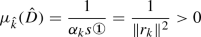
  and therefore no negative curvature direction can be provided from the current step ${\hat{k}}$.

• (IV) As a final subcase, we assume ${\hat{k}} = k+1$, i.e., by (25) . Again, since ${\hat{D}}$ is diagonal, then the linear system (29) reduces to ${\hat{L}}^T y = e_{{\hat{k}}}$ (or equivalently ${\hat{L}}^T y = e_{k+1}$), with

  $$\begin{aligned} \begin{array}{l} -\sqrt{\beta _1} \cdot y_2 + y_1= 0 \\ \qquad \vdots \\ -\sqrt{\beta _{k -1}} \cdot y_{k} + y_{k -1} = 0 \\ \frac{\Vert r_k\Vert \sqrt{\beta _k \lambda _k}}{\sqrt{\beta _k + \lambda _k^2}} \cdot y_k + \frac{\Vert r_k\Vert \lambda _k\sqrt{\lambda _k}}{\sqrt{\beta _k + \lambda _k^2}} \cdot y_{k+1} \\ \, - \frac{\Vert Ap_k\Vert \Vert r_{k+2}\Vert }{\Vert r_{k}\Vert } \sqrt{\frac{\lambda _k}{\beta _k + \lambda _k^2}} \cdot y_{k+2} = 0 \\ \frac{\sqrt{-\lambda _{k+1} \beta _k}}{\Vert Ap_k\Vert \sqrt{\beta _k + \lambda _{k+1}^2}} \cdot y_k + \frac{\lambda _{k+1} \sqrt{-\lambda _{k+1}}}{\Vert Ap_k\Vert \sqrt{\beta _k + \lambda _{k+1}^2}} \cdot y_{k+1} \\ \, - \frac{\Vert r_{k+2}\Vert }{\Vert r_k\Vert ^2}\sqrt{-\frac{\lambda _{k+1}}{\beta _k + \lambda _{k+1}^2}} \cdot y_{k+2} = 1 \\ -\sqrt{\beta _{k+2}} \cdot y_{k+3} + y_{k+2} = 0 \\ \qquad \vdots \\ -\sqrt{\beta _{n-1}} \cdot y_{n} + y_{n-1} = 0 \\ y_n = 0. \end{array} \end{aligned}$$

  Now, we have for the last $n - {\hat{k}}$ entries of vector ${\hat{y}}$ the expression

  $$\begin{aligned} {\hat{y}}_n = \cdots = {\hat{y}}_{{\hat{k}}+1}=0. \end{aligned}$$

  On the other hand, the condition ${\hat{y}}_{{\hat{k}} +1} = {\hat{y}}_{k+2}=0$ and the above relation

  $$\begin{aligned} \frac{\Vert r_k\Vert \sqrt{\beta _k \lambda _k}}{\sqrt{\beta _k + \lambda _k^2}} \cdot y_k + \frac{\Vert r_k\Vert \lambda _k\sqrt{\lambda _k}}{\sqrt{\beta _k + \lambda _k^2}} \cdot y_{k+1} - \frac{\Vert Ap_k\Vert \Vert r_{k+2}\Vert }{\Vert r_{k}\Vert } \sqrt{\frac{\lambda _k}{\beta _k + \lambda _k^2}} \cdot y_{k+2} = 0 \end{aligned}$$

  yield

  $$\begin{aligned} {\hat{y}}_k = - \frac{\lambda _k}{\sqrt{\beta _k}} {\hat{y}}_{k + 1}. \end{aligned}$$

  Recalling that now ${\hat{k}} = k+1$ and in Table 3$\Vert Ap_k\Vert =\Vert r_{k+1}\Vert = \Vert r_{{\hat{k}}}\Vert$, then

  $$\begin{aligned} {\hat{y}}_{k + 1} = \frac{\Vert r_{{\hat{k}}}\Vert }{\lambda _{k +1} - \lambda _k} \sqrt{\frac{\beta _k + \lambda _{k+1}^2}{-\lambda _{k+1}}}. \end{aligned}$$

  As a consequence,

  $$\begin{aligned} {\hat{y}}_k = - \frac{\lambda _k}{\sqrt{\beta _k}} \cdot \frac{\Vert r_{{\hat{k}}}\Vert }{\lambda _{k +1} - \lambda _k} \sqrt{\frac{\beta _k + \lambda _{k+1}^2}{-\lambda _{k+1}}} = - \frac{\lambda _k \Vert r_{{\hat{k}} - 1}\Vert }{\lambda _{k +1} - \lambda _k} \sqrt{\frac{\beta _k + \lambda _{k+1}^2}{-\lambda _{k+1}}} \end{aligned}$$

  and for ${\hat{y}}_{{\hat{k}} -2}, \ldots , {\hat{y}}_1$, we have

  $$\begin{aligned} {\hat{y}}_i = - \frac{\Vert r_{{\hat{k}}-1}\Vert ^2}{\Vert r_i\Vert } \cdot \frac{\lambda _k}{\lambda _{k +1} - \lambda _k} \sqrt{\frac{\beta _k + \lambda _{k+1}^2}{-\lambda _{k+1}}}, \qquad i = {\hat{k}} -2, \ldots ,1. \end{aligned}$$

  Finally, the overall negative curvature direction $d_j$ becomes now

  $$\begin{aligned} d_j= & {} R_j {\hat{y}} \\= & {} \Vert r_{{\hat{k}} -1}\Vert ^2 \left[ \sum _{i=1}^{{\hat{k}}-2} - \frac{r_i}{\Vert r_i\Vert ^2} \cdot \frac{\lambda _k}{\lambda _{k +1} - \lambda _k} \sqrt{\frac{\beta _k + \lambda _{k+1}^2}{-\lambda _{k+1}}} \right] \\&\qquad - \frac{1}{\lambda _{k +1} - \lambda _k} \sqrt{\frac{\beta _k + \lambda _{k+1}^2}{-\lambda _{k+1}}} \left( \lambda _{{\hat{k}}-1} r_{{\hat{k}}-1} -r_{{\hat{k}}} \right) \\= & {} -\frac{\lambda _k}{\lambda _{k +1} - \lambda _k} \sqrt{\frac{\beta _k + \lambda _{k+1}^2}{-\lambda _{k+1}}} \beta _{k-1}p_{k-1} \\&\qquad - \frac{1}{\lambda _{k +1} - \lambda _k} \sqrt{\frac{\beta _k + \lambda _{k+1}^2}{-\lambda _{k+1}}} (\lambda _k r_k - r_{k+1}) \\= & {} -\frac{\lambda _k}{\lambda _{k +1} - \lambda _k} \sqrt{\frac{\beta _k + \lambda _{k+1}^2}{-\lambda _{k+1}}} \left[ \beta _{k-1}p_{k-1} + r_k - \frac{r_{k+1}}{\lambda _k} \right] \\= & {} -\frac{\lambda _k}{\lambda _{k +1} - \lambda _k} \sqrt{\frac{\beta _k + \lambda _{k+1}^2}{-\lambda _{k+1}}} \left[ p_k - \frac{Ap_k}{\lambda _k} \right] , \end{aligned}$$

  whose computation is well posed, since $\lambda _{k+1} <0$. Again, by (20)–(21), the fact that ${\bar{\lambda }} > 0$ in Lemma 4.1 and the other hypotheses, the quantity $\Vert d_j\Vert$ is bounded. In addition, the computation of $d_j$ evidently needs the storage of just two n-real vectors. $\square$

Observation 5.1

We remark that the computation of the negative curvature direction $d_j$ requires at most the additional storage of a couple of vectors, which confirms the competitiveness of the storage proposed in [9]. Thus, the approach in this paper does not only prove to be applicable to large-scale problems, but it also simplifies the theory in [9], which is currently in our knowledge the only proposal of iterative computation of negative curvatures for large-scale problems, which does not need any recomputing (as in [3]), and which requires neither a full matrix factorization nor any matrix storage.

6 Numerical Experience

In this section, we report the results of a numerical experience concerning the adoption of our approach, within the framework of truncated Newton methods for large-scale unconstrained optimization. We considered the truncated Newton method proposed in [9], where we replaced the Krylov-based iterative procedure therein by the procedure. The codes were written in Fortran compiled with Gfortran 6 under Linux Ubuntu 18.04, and the runs were performed on a PC with Intel Core i7-4790K quad-core 4.00 GHz Processor and 32 GB RAM.

Now we strongly remark the guidelines and the limits of the numerical experience reported in this section:

• we show how to detect and assess negative curvatures for the Hessian matrix $\nabla ^2 f(x_j)$, at the current iterate $x_j$;

• we compute negative curvatures which could be able to guarantee the overall convergence of the optimization method toward second-order critical points;

• we do not claim that our proposal shows better numerical results with respect to [9], being the main focus of this paper on theoretical issues. Thus, our numerical experience only tests the reliability and the effectiveness of our method, rather than proposing a numerical comparison with the current literature;

• we also intend to check for the quality of the stationary points detected by our approach.

In particular, we considered all the 112 large-scale unconstrained test problems in CUTEst [54] suite. The algorithm performs a classic nested loop of outer–inner iterations. Thus, at the current jth outer iteration the algorithm iteratively solves Newton’s equation $\nabla ^2f(x_j)s=-\nabla f(x_j)$, performing a certain number of inner iterations. To build an approximate solution $s_j$ of Newton’s equation, and possibly a negative curvature direction, inner iterations are stopped whenever the following truncation rule is satisfied

$$\begin{aligned} \Vert \nabla ^2f(x_j)s_j + \nabla f(x_j)\Vert \le \eta _j \Vert \nabla f(x_j)\Vert , \end{aligned}$$

being $\{\eta _j\}$ a forcing sequence, with $\eta _j \rightarrow 0$. The condition $\eta _j \rightarrow 0$ guarantees superlinear convergence of the overall method, when close enough to the final stationary point. As regards settings and parameters of the linesearch procedure we adopted, as well as the overall stopping criterion, the reader can refer to [9]. (We also recall that, unlike in [9], here we preferred not to include any nonmonotonicity in the used algorithm, in order to clearly distinguish the contribution from our idea.) At each inner iteration $k\ge 1$, the algorithm in Table 2 detects a curvature of the objective function, by computing the term $p_k^T \nabla ^2f(x_j) p_k$, a negative value of the last quantity indicating a negative curvature direction.

We compared two truncated Newton methods: the first (i) not including the use of negative curvature directions (namely NoNegCurv), so that convergence to simple stationary points could be guaranteed; the second (ii) including negative curvatures (namely NegCurv) which satisfy Assumption 2.1, implying convergence to stationary points where second-order necessary optimality conditions are fulfilled. Thus, by a comparison between them, we might have expected:

• (a) (ii) to be more efficient than (i) in terms of the computational effort (in our large-scale setting we measured the computational effort through the number of inner iterations, which are representative of the overall computational burden, including CPU time);

• (b) the quality of the solutions detected by (ii), i.e., the value of the objective function at the solution, is expected to be on average not worse than in the case of (i), since for (ii) the solution points satisfy additional theoretical properties;

• (c) the stationarity (measured by $\Vert \nabla f(x^*)\Vert$) of the final solution detected using (ii) is possibly expected to be competitive with respect to (i). This is because in a neighborhood of the solution point, our proposal is expected to collect more information on the objective function.

The above considerations are to large extent confirmed by our numerical experience as detailed in the following.

First, note that using (ii), we detected negative curvatures on 40 test problems out of 112; of course, this does not imply that the remaining 72 test problems only include convex functions. It rather implies that on 72 problems, no regions of concavity for the objective function were encountered. For these 40 test problems, the obtained results in terms of number of (outer) iterations (it), number of function evaluations (nf), number of inner iterations (inner-it), optimal function value ($f(x^*)$), gradient norm at the optimal point ($\Vert g(x^*)\Vert$), solution time in seconds (time), are reported in Tables 4 and 5. In particular, for each test problem, we report results using both the NoNegCurv method (top row) and the NegCurv method (bottom row).

Table 4 Complete results for CUTEst test problems where negative curvature directions are encountered. For each test problem, results for NoNegCurv (top row) and NegCurv (bottom row) are reported. Part 1

Table 5 Complete results for CUTEst test problems where negative curvature directions are encountered. For each test problem, results for NoNegCurv (top row) and NegCurv (bottom row) are reported. Part 2

By observing these results, we first note that on two test problems both the algorithms fail to converge within the maximum CPU time of 900 s. The comparison on the remaining test problems shows that in most cases algorithm NegCurv performs the best in terms of solution time and inner iterations, confirming expectation (a) which is our main goal. The results highlight only one test problem (GENHUPMS 1000) where the use of NegCurv yields a significant worsening of the performance. We easily realize that including our procedure to compute negative curvature directions allows to both speed up the overall convergence and decrease the number of inner iterations.

The detailed results only partially validate also (b) and (c). As regards (b), since in a few test problems the algorithms converge to different points, a sound statistical analysis cannot be given, though a better optimal value is sometimes observed by using NegCurv algorithm. Similarly, as concerns (c), the values of $\Vert \nabla f(x^*)\Vert$ provided by NoNegCurv and NegCurv seem to a large extent comparable on this test set.

To have an overview of the effectiveness and the robustness of the approach we propose in this paper, we now consider summary results by using performance profiles [55]. The performance profiles represent a popular and widely used tool for providing objective information when benchmarking optimization algorithms. Their meaning can be summarized as follows: Suppose you have a set of solvers ${{\mathcal {S}}}$ to be compared on a set of test problems ${{\mathcal {P}}}$.

For each problem $p\in {{\mathcal {P}}}$ and solver $s\in {{\mathcal {S}}}$, define $t_{ps}$ the statistic obtained by running solver s on problem p. Namely, $t_{ps}\ge 0$ is a performance measure of interest, e.g., solution time, number of function evaluations, etc. The performance on problem p by solver s is compared with the best performance by any solver on this problem by means of the performance ratio

$$\begin{aligned} r_{ps}= \frac{t_{ps}}{\{t_{ps} ~| ~ s\in {{\mathcal {S}}}\}}. \end{aligned}$$

Moreover, an upper bound ${{\bar{r}}}$ is chosen such that $r_{ps}\le {\bar{r}}$ for all $s\in {{\mathcal {S}}}$ and $p\in {{\mathcal {P}}}$ and if a solver s fails to solve problem p then $r_{ps}$ is set to ${\bar{r}}$. The performance profile of the solver s is the function

$$\begin{aligned} \rho _s(\tau ) = \frac{\left| \{p\in {{\mathcal {P}}} ~ | ~ t_{ps}\le \tau \}\right| }{\left| {{\mathcal {S}}} \right| }, \end{aligned}$$

namely the cumulative distribution function for the performance ratio.

In particular, we report in Figs. 1 (full profile) and 2 (detail profile) the performance profiles comparing NoNegCurv and NegCurv algorithms in terms of inner iterations. The test set considered includes the 40 test problems reported in Tables 4 and 5.

Fig. 1

Performance profile relative to a comparison between (ii) and (i), with respect to the number of inner iterations, where negative curvatures are (red line)/are not (green dashed line) used (full profile)

Fig. 2

Performance profile relative to a comparison between (ii) and (i), with respect to the number of inner iterations, where negative curvatures are (red line)/are not (green dashed line) used (detail profile)

The detailed plot reported in Fig. 2 clearly shows the effectiveness of NegCurv algorithm with respect to NoNegCurv. Indeed, as an example, let us consider the value of abscissa 1.2 in Fig. 2. The plots show that the NegCurv algorithm is able to solve about $62\%$ of the test problems within 1.2 times the number of inner iterations of the best algorithm. Conversely, the NoNegCurv algorithm is able to solve up to $78\%$ of the test problems within the same number of inner iterations. On the other hand, in terms of robustness the algorithms can be considered comparable with a slight preference for NegCurv algorithm as evidenced by Fig. 1. The last consideration follows from the observation that for values of the abscissa parameter larger than 3.5, the two plots basically tend to overlap.

7 Conclusions

We proposed a novel approach for the efficient solution of large-scale unconstrained optimization problems, where the detected solutions likely are endowed with strong theoretical properties. Our proposal exploits the simplicity of an algebra associated with the numeral grossone, which was recently introduced in the literature to handle infinite and infinitesimal quantities.

We were able to extend the results in [9] in view of a theoretical simplification, avoiding to make reference to Planar-CG methods which require a more complex analysis. The theory in this paper allows us to guarantee that the iterative computation of negative curvatures does not need any matrix storage, while preserving convergence toward points satisfying second-order necessary optimality conditions.

Then, we also provided numerical results, which show the efficiency of our proposal. We remark that the focus of this paper is not on a numerical comparison among different algorithms which exploit negative curvature directions. Rather, we paired the approach in [9] with a novel paradigm provided by grossone, in light of preserving numerical efficiency within a sound theoretical framework, in dealing with nonconvex problems. This is the first stage toward a more complete numerical experience where the iterative algorithm can be fully tested, including even more challenging problems from real-world applications.

Observe that the proposed approach is independent under multiplication of the function by a positive scaling constant or adding a shifting constant. This is an important property that is specially exploited in the global optimization framework (see, e.g., [24]), since strongly homogeneous algorithms are definitely appealing. Furthermore, the local solver described in Sect. 6 may be considered to enhance the efficiency of the algorithm in [56], simply replacing the local solver used therein by our proposal.

References

Ferris, M., Lucidi, S., Roma, M.: Nonmonotone curvilinear line search methods for unconstrained optimization. Comput. Optim. Appl. 6, 117–136 (1996)
Goldfarb, D.: Curvilinear path steplength algorithms for minimization which use directions of negative curvature. Math. Program. 18(1), 31–40 (1980)
Gould, N.I.M., Lucidi, S., Roma, M., Toint, P.L.: Exploiting negative curvature directions in linesearch methods for unconstrained optimization. Optim. Methods Softw. 14, 75–98 (2000)
Goldfarb, D., Mu, C., Wright, J., Zhou, C.: Using negative curvature in solving nonlinear programs. Comput. Optim. Appl. 68(3), 479–502 (2017)
Lucidi, S., Rochetich, F., Roma, M.: Curvilinear stabilization techniques for truncated Newton methods in large-scale unconstrained optimization. SIAM J. Optim. 8, 916–939 (1998)
McCormick, G.P.: A modification of Armijo’s step-size rule for negative curvature. Math. Program. 13(1), 111–115 (1977)
Moré, J., Sorensen, D.: On the use of directions of negative curvature in a modified Newton method. Math. Program. 16, 1–20 (1979)
Curtis, F., Robinson, D.: Exploiting negative curvature in deterministic and stochastic optimization. Math. Program. 176, 69–94 (2019)
Fasano, G., Roma, M.: Iterative computation of negative curvature directions in large scale optimization. Comput. Optim. Appl. 38(1), 81–104 (2007)
Fasano, G., Lucidi, S.: A nonmonotone truncated Newton–Krylov method exploiting negative curvature directions, for large scale unconstrained optimization. Optim. Lett. 3(4), 521–535 (2009)
Hestenes, M.R., Stiefel, E.L.: Methods of conjugate gradients for solving linear systems. J. Res. Nat. Bur. Stand. 49, 409–436 (1952)
De Leone, R., Fasano, G., Sergeyev, Y.D.: Planar methods and grossone for the conjugate gradient breakdown in nonlinear programming. Comput. Optim. Appl. 71, 73–93 (2018)
Sergeyev, Y.D.: Numerical infinities and infinitesimals: methodology, applications, and repercussions on two Hilbert problems. EMS Surv. Math. Sci. 4(2), 219–320 (2017)
Fasano, G.: Conjugate gradient (CG)-type method for the solution of Newton’s equation within optimization frameworks. Optim. Methods Softw. 19(3–4), 267–290 (2004)
Lolli, G.: Metamathematical investigations on the theory of grossone. Appl. Math. Comput. 255, 3–14 (2015)
Margenstern, M.: Using Grossone to count the number of elements of infinite sets and the connection with bijections. p-Adic Numbers Ultrametric Anal. Appl. 3(3), 196–204 (2011)
Montagna, F., Simi, G., Sorbi, A.: Taking the Pirahã seriously. Commun. Nonlinear Sci. Numer. Simul. 21(1–3), 52–69 (2015)
Sergeyev, Y.D.: Computer system for storing infinite, infinitesimal, and finite quantities and executing arithmetical operations with them. USA patent 7,860,914 (2010)
Cococcioni, M., Cudazzo, A., Pappalardo, M., Sergeyev, Y.D.: Solving the lexicographic multi-objective mixed-integer linear programming problem using branch-and-bound and Grossone methodology. Commun. Nonlinear Sci. Numer. Simul. 84, 105177 (2020)
Cococcioni, M., Pappalardo, M., Sergeyev, Y.D.: Lexicographic multi-objective linear programming using grossone methodology: theory and algorithm. Appl. Math. Comput. 318, 298–311 (2018)
De Cosmis, S., Leone, R.D.: The use of grossone in mathematical programming and operations research. Appl. Math. Comput. 218(16), 8029–8038 (2012)
De Leone, R.: Nonlinear programming and grossone: quadratic programming and the role of constraint qualifications. Appl. Math. Comput. 318, 290–297 (2018)
Gaudioso, M., Giallombardo, G., Mukhametzhanov, M.S.: Numerical infinitesimals in a variable metric method for convex nonsmooth optimization. Appl. Math. Comput. 318, 312–320 (2018)
Sergeyev, Y.D., Kvasov, D.E., Mukhametzhanov, M.S.: On strong homogeneity of a class of global optimization algorithms working with infinite and infinitesimal scales. Commun. Nonlinear Sci. Numer. Simul. 59, 319–330 (2018)
Caldarola, F.: The Sierpinski curve viewed by numerical computations with infinities and infinitesimals. Appl. Math. Comput. 318, 321–328 (2018)
Sergeyev, Y.D.: Numerical point of view on Calculus for functions assuming finite, infinite, and infinitesimal values over finite, infinite, and infinitesimal domains. Nonlinear Anal. Ser. A Theory Methods Appl. 71(12), e1688–e1707 (2009)
Sergeyev, Y.D.: Numerical infinities applied for studying Riemann series theorem and Ramanujan summation. In: AIP Conference Proceedings of ICNAAM 2017, vol. 1978, p. 020004. AIP Publishing, New York (2018). https://doi.org/10.1063/1.5043649
Zhigljavsky, A.: Computing sums of conditionally convergent and divergent series using the concept of grossone. Appl. Math. Comput. 218(16), 8064–8076 (2012)
Caldarola, F.: The exact measures of the Sierpinski d-dimensional tetrahedron in connection with a diophantine nonlinear system. Commun. Nonlinear Sci. Numer. Simul. 63, 228–238 (2018)
D’Alotto, L.: A classification of two-dimensional cellular automata using infinite computations. Indian J. Math. 55, 143–158 (2013)
Sergeyev, Y.D.: Evaluating the exact infinitesimal values of area of Sierpinski’s carpet and volume of Menger’s sponge. Chaos Solitons Fractals 42(5), 3042–3046 (2009)
Falcone, A., Garro, A., Mukhametzhanov, M.S., Sergeyev, Y.D.: A simulink-based infinity computer simulator and some applications. Lecture Notes in Computer Science 11974 LNCS, pp. 362–369 (2020). https://doi.org/10.1007/978-3-030-40616-5_31
Iudin, D.I., Sergeyev, Y.D., Hayakawa, M.: Infinity computations in cellular automaton forest-fire model. Commun. Nonlinear Sci. Numer. Simul. 20(3), 861–870 (2015)
Margenstern, M.: Fibonacci words, hyperbolic tilings and grossone. Commun. Nonlinear Sci. Numer. Simul. 21(1–3), 3–11 (2015)
Sergeyev, Y.D.: Counting systems and the First Hilbert problem. Nonlinear Anal. Ser. A Theory Methods Appl. 72(3–4), 1701–1708 (2010)
Sergeyev, Y.D., Garro, A.: Single-tape and multi-tape Turing machines through the lens of the Grossone methodology. J. Supercomput. 65(2), 645–663 (2013)
Fiaschi, L., Cococcioni, M.: Numerical asymptotic results in game theory using Sergeyev’s Infinity Computing. Int. J. Unconv. Comput. 14(1), 1–25 (2018)
Rizza, D.: A study of mathematical determination through Bertrand’s Paradox. Philosophia Mathematica 26(3), 375–395 (2018)
Rizza, D.: Numerical methods for infinite decision-making processes. Int. J. Unconv. Comput. 14(2), 139–158 (2019)
Amodio, P., Iavernaro, F., Mazzia, F., Mukhametzhanov, M., Sergeyev, Y.D.: A generalized Taylor method of order three for the solution of initial value problems in standard and infinity floating-point arithmetic. Math. Comput. Simul. 141, 24–39 (2017)
Sergeyev, Y.D.: Higher order numerical differentiation on the Infinity Computer. Optim. Lett. 5(4), 575–585 (2011)
Iavernaro, F., Mazzia, F., Mukhametzhanov, M.S., Sergeyev, Y.D.: Conjugate-symplecticity properties of Euler–Maclaurin methods and their implementation on the Infinity Computer. Appl. Numer. Math. 155, 58–72 (2020). https://doi.org/10.1016/j.apnum.2019.06.011
Sergeyev, Y.D., Mukhametzhanov, M.S., Mazzia, F., Iavernaro, F., Amodio, P.: Numerical methods for solving initial value problems on the Infinity Computer. Int. J. Unconv. Comput. 12(1), 3–23 (2016)
Sergeyev, Y.D.: Independence of the grossone-based infinity methodology from non-standard analysis and comments upon logical fallacies in some texts asserting the opposite. Found. Sci. 24(1), 153–170 (2019)
Golub, G.H., Loan, C.F.V.: Matrix Computations, 4th edn. The Johns Hopkins University Press, Baltimore (2013)
Paige, C., Saunders, M.: Solution of sparse indefinite systems of linear equations. SIAM J. Numer. Anal. 12, 617–29 (1975)
HSL\_MI02 Symmetric possibly-indefinite system: SYMMBK method. Harwell Mathematical Software Library http://www.hsl.rl.ac.uk (2013)
Fasano, G.: Planar-conjugate gradient algorithm for large scale unconstrained optimization, part 1: theory. J. Optim. Theory Appl. 125(3), 523–541 (2005)
Fasano, G.: Planar-conjugate gradient algorithm for large scale unconstrained optimization, part 2: application. J. Optim. Theory Appl. 125(3), 543–558 (2005)
Fasano, G.: Lanczos-conjugate gradient method and pseudoinverse computation, on indefinite and singular systems. J. Optim. Theory Appl. 132(2), 267–285 (2007)
Nash, S.G.: A survey of truncated-Newton methods. J. Comput. Appl. Math. 124, 45–59 (2000)
Fasano, G.: Planar-CG methods and matrix tridiagonalization in large scale unconstrained optimization. In: Di Pillo, G., Murli, A. (eds.) High Performance Algorithms and Software for Nonlinear Optimization, pp. 243–263. Kluwer Academic Publishers, Dordrecht (2003)
Fasano, G., Pesenti, R.: Conjugate direction methods and polarity for quadratic hypersurfaces. J. Optim. Theory Appl. 175, 764–794 (2017)
Gould, N.I.M., Orban, D., Toint, P.L.: CUTEst: a constrained and unconstrained testing environment with safe threads. Comput. Optim. Appl. 60, 545–557 (2015)
Dolan, E.D., Moré, J.: Benchmarking optimization software with performance profiles. Math. Program. 91, 201–213 (2002)
Žilinskas, A., Gillard, J., Scammell, M., Zhigljavsky, A.: Multistart with early termination of descents. J. Global Optim. (2019). https://doi.org/10.1007/s10898-019-00814-w
Acknowledgements
Open access funding provided by Università Ca’ Foscari Venezia within the CRUI-CARE Agreement. G. Fasano thanks the National Research Council-Marine Technology Research Institute (CNR-INSEAN), Italy, for the support received. R. De Leone, G. Fasano, M. Roma and Yaroslav D. Sergeyev are grateful to the National Research Group GNCS (Gruppo Nazionale per il Calcolo Scientifico) within IN\(\delta \)AM, Istituto Nazionale di Alta Matematica, Italy. The authors wish to thank both the reviewers for their fruitful and constructive comments.
Author information
Authors and Affiliations
Corresponding author
Additional information
Communicated by Alexandre Cabot.
Publisher's Note
Springer Nature remains neutral with regard to jurisdictional claims in published maps and institutional affiliations.
Rights and permissions
Open Access This article is licensed under a Creative Commons Attribution 4.0 International License, which permits use, sharing, adaptation, distribution and reproduction in any medium or format, as long as you give appropriate credit to the original author(s) and the source, provide a link to the Creative Commons licence, and indicate if changes were made. The images or other third party material in this article are included in the article’s Creative Commons licence, unless indicated otherwise in a credit line to the material. If material is not included in the article’s Creative Commons licence and your intended use is not permitted by statutory regulation or exceeds the permitted use, you will need to obtain permission directly from the copyright holder. To view a copy of this licence, visit http://creativecommons.org/licenses/by/4.0/.
About this article
Cite this article
De Leone, R., Fasano, G., Roma, M. et al. Iterative Grossone-Based Computation of Negative Curvature Directions in Large-Scale Optimization. J Optim Theory Appl 186, 554–589 (2020). https://doi.org/10.1007/s10957-020-01717-7
Received:
Accepted:
Published:
Issue Date:
DOI: https://doi.org/10.1007/s10957-020-01717-7
Keywords
- Negative curvature directions
- Second-order necessary optimality conditions
- Grossone
- Conjugate gradient method