Interface Dynamics of a Metastable Mass-Conserving Spatially Extended Diffusion

Abstract

We study the metastable dynamics of a discretised version of the mass-conserving stochastic Allen–Cahn equation. Consider a periodic one-dimensional lattice with N sites, and attach to each site a real-valued variable, which can be interpreted as a spin, as the concentration of one type of metal in an alloy, or as a particle density. Each of these variables is subjected to a local force deriving from a symmetric double-well potential, to a weak ferromagnetic coupling with its nearest neighbours, and to independent white noise. In addition, the dynamics is constrained to have constant total magnetisation or mass. Using tools from the theory of metastable diffusion processes, we show that the long-term dynamics of this system is similar to a Kawasaki-type exchange dynamics, and determine explicit expressions for its transition probabilities. This allows us to describe the system in terms of the dynamics of its interfaces, and to compute an Eyring–Kramers formula for its spectral gap. In particular, we obtain that the spectral gap scales like the inverse system size squared.

Appendices

Appendix 1: Proofs: Potential Landscape

1.1 The Uncoupled Case

Proof of Proposition 3.1

Consider a critical point $x^\star$ of the constrained system with triple $(a_0,a_1,a_2)$. Recall that this means that $x^\star$ has $a_j$ coordinates equal to $\alpha _j$, $j=0,1,2$, where the $\alpha _j$ are distinct roots of $\xi ^3-\xi -\lambda$ for some $\lambda \in (-\lambda _{\text{ c }},\lambda _{\text{ c }})$. By Vieta’s formula, these roots satisfy

$$\begin{aligned} \alpha _0 + \alpha _1 + \alpha _2 = 0. \end{aligned}$$

(7.1)

We always have $a_0+a_1+a_2=N$, and by convention $a_0\le a_1\le a_2$. Note that we may assume $a_0\ne a_2$, since otherwise all $a_j$ would be equal, and thus N would be a multiple of 3, which is excluded by assumption.

Combining (7.1) with the constraint $\sum x^\star _i = a_0\alpha _0 + a_1\alpha _1 + a_2\alpha _2 = 0$ yields the relation

$$\begin{aligned} (a_1-a_0)\alpha _1 + (a_2-a_0)\alpha _2 = 0. \end{aligned}$$

(7.2)

Solving for $\alpha _2$ and using the fact that all $\alpha _j^3-\alpha _j$ are equal, a short computation shows that

$$\begin{aligned} \alpha _0&= \pm (a_1-a_2) R^{1/2}, \nonumber \\ \alpha _1&= \pm (a_2-a_0) R^{1/2}, \\ \alpha _2&= \pm (a_0-a_1) R^{1/2}, \nonumber \end{aligned}$$

(7.3)

where

$$\begin{aligned} R = \frac{a_2+a_1-2a_0}{(a_1-a_0)^3+(a_2-a_0)^3} = \frac{1}{a_0^2+a_1^2+a_2^2-a_0a_1-a_0a_2-a_1a_2}. \end{aligned}$$

(7.4)

We now turn to determining the signature of the Hessian at these critical points of the potential $V_\gamma$ restricted to the hyperplane S. This signature does not depend on the parametrisation of S, so that it is equal to the signature of the Hessian of

$$\begin{aligned} \widetilde{V}_\gamma (x_1,\dots ,x_{N-1}) = V_\gamma (x_1,\dots ,x_{N-1},-x_1-\dots -x_{N-1}). \end{aligned}$$

(7.5)

Computing the Hessian of $\widetilde{V}_\gamma$ at $x^\star$ shows that it has the form

(7.6)

where ${1}\mathrm{l}_a$ denotes the identity matrix of size a. We now distinguish between the following cases.

• 1. $(a_0,a_1,a_2)=(0,0,N)$. Then $x^\star =0$, and one easily sees that $-H$ is positive definite, so that $x^\star$ is a saddle of index $N-1$.

• 2. $a_0=0$ and $a_1\ge 1$. Using the expressions (7.3), we obtain that $3\alpha _1^2-1>0$ and $3\alpha _2^2-1$ has the same sign as $2a_1-a_2$. Let $e_1, \dots , e_{N-1}$ denote the canonical basis vectors. Then $\{e_1-e_i\}_{i\in \llbracket 2,a_1\rrbracket }$ are eigenvectors of H with eigenvalue $3\alpha _1^2-1$, and $\{e_{a_1+1}-e_i\}_{i\in \llbracket a_1+2,N-1\rrbracket }$ are eigenvectors of H with eigenvalue $3\alpha _2^2-1$.

  To find the remaining two eigenvalues, let $u=\sum _{i=1}^{a_1}e_i$ and $v=\sum _{i=a_1+1}^{N-1}e_i$. These two vectors span an invariant subspace of H, in which the action of H takes the form

  

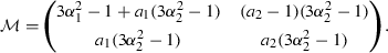  (7.7)

  Computing the determinant and the trace of ${\mathcal M}$, one sees that if $2a_1>a_2$, then the two eigenvalues of ${\mathcal M}$ are strictly positive, so that $x^\star$ is a stationary point of index 0. If $2a_1<a_2$, then ${\mathcal M}$ has one strictly positive and one strictly negative eigenvalue, and $x^\star$ has index $a_2-1$.

• 3. $a_0\ge 1$. In that case one finds that $3\alpha _1^2-1>0$, while $3\alpha _0^2-1$ has the same sign as $(2a_2-a_1-a_0)(a_0-2a_1+a_2)$ and $3\alpha _2^2-1$ has the same sign as $(2a_0-a_1-a_2)(a_0-2a_1+a_2)$. Here it is better to invert the rôles of $\alpha _1$ and $\alpha _2$ in the expression for H. Similarly to the previous case, one finds $a_0-1$ eigenvectors with eigenvalue $3\alpha _0^2-1$, $a_2-1$ eigenvectors with eigenvalue $3\alpha _2^2-1$ and $a_1-2$ eigenvectors with eigenvalue $3\alpha _1^2-1$ (these eigenvectors are of the form $e_1-e_i$, $e_{a_0+1}-e_i$ and $e_{a_0+a_2+1}-e_i$ for appropriate ranges of i).

  To find the other eigenvalues, let $u=\sum _{i=1}^{a_0}e_i$, $v=\sum _{i=a_0+1}^{a_0+a_2}e_i$ and $w=\sum _{i=a_0+a_2+1}^{N-1}e_i$. These span an H-invariant subspace, in which the action of H takes the form

  

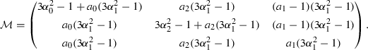  (7.8)

  In this case, one finds ${{\mathrm{Tr}}}{\mathcal M}>0$, and $\det {\mathcal M}$ has the same sign as $a_0-2a_1+a_2$. If $\det {\mathcal M}<0$, then ${\mathcal M}$ has two strictly positive and one strictly negative eigenvalue, and $x^\star$ has index $a_0$. If $\det {\mathcal M}>0$, computing the term of degree 1 of the characteristic polynomial of ${\mathcal M}$ one concludes that all eigenvalues of ${\mathcal M}$ are strictly positive, and that $x^\star$ has index $a_2-1$. $\square$

Proof of Theorem 3.5

Let $z^\star \in C_k$ be a 1-saddle. Its triple can be written $(1,a-1,N-a)$ where $a=\frac{N}{2}-k+1 \in \llbracket \frac{N}{2}+1-k_{\max },\frac{N}{2}\rrbracket$. We shall construct a path $\Gamma$, connecting $z^\star$ to a point $x^\star \in B_{k-1}$ of triple $(0,a,N-a)$, and such that the potential $V_0$ is decreasing along $\Gamma$. An analogous construction holds for the connection from $z^\star$ to a local minimum in $B_k$.

In fact it will turn out to be sufficient to use a linear path. Reordering the components if necessary, we may assume that $x^\star =(\alpha _1,\dots ,\alpha _1,\alpha _2,\dots ,\alpha _2)$ with $\alpha _1$ repeated a times and $\alpha _2$ repeated $N-a$ times, and $z^\star =(\alpha '_0,\alpha '_1,\dots ,\alpha '_1,\alpha '_2,\dots ,\alpha '_2)$, with $\alpha '_1$ repeated $a-1$ times and $\alpha '_2$ repeated $N-a$ times. Note that these points indeed satisfy the connection rules (3.5). Let $\Gamma (t)=tz^\star + (1-t)x^\star$ and set $h(t)=V_0(\Gamma (t))$. Then a direct computation shows that

$$\begin{aligned} h'(t)&= (\alpha _0'-\alpha _1) \bigl [((1-t)\alpha _1+t\alpha '_0)^3 - ((1-t)\alpha _1+t\alpha _0')\bigr ] \nonumber \\&\quad \,+ (a-1)(\alpha _1'-\alpha _1) \bigl [((1-t)\alpha _1+t\alpha '_1)^3 - ((1-t)\alpha _1+t\alpha _1')\bigr ] \nonumber \\&\quad \,+ (N-a)(\alpha _2'-\alpha _2) \bigl [((1-t)\alpha _2+t\alpha '_2)^3 - ((1-t)\alpha _2+t\alpha _2')\bigr ]. \end{aligned}$$

(7.9)

The properties of the $\alpha _j$ and $\alpha '_j$ yield $h'(0)=h'(1)=0$. Since $h'(t)$ is a polynomial of degree 3, it can be written as

$$\begin{aligned} h'(t) = Kt(t-1)(t-\psi ) \end{aligned}$$

(7.10)

for some $K, \psi \in \mathbb {R}$. Computing the coefficient of $t^3$ in (7.9) yields $K>0$. Thus if we manage to show that $\psi >1$, we can indeed conclude that $h'(t)<0$ on (0, 1), showing that h(t) is decreasing as required. The condition $\psi >1$ is equivalent to having $h''(1)<0$. Using the expressions (7.3) of the $\alpha _j$, one obtains after some algebra that

$$\begin{aligned} h''(1)&= 2(\omega ')^2 \bigl [(a-1)(9a-8N)+aN^2-a^2N\bigr ] -4\omega \omega 'N(N-a)(a-2) \nonumber \\&\quad -\omega ^2aN(N-a) + 3(\omega \omega ')^2(N-a) \bigl [aN^3-3a^2N^2+3Na^2\nonumber \\&\quad - (a-1)(9a^2-9aN+4N^2)\bigr ], \end{aligned}$$

(7.11)

where $\omega =(N^2-3aN+3a^2)^{-1/2}$ and $\omega '=(N^2-3aN+3(a^2-a+1))^{-1/2}$ stem from the terms $R^{1/2}$ in (7.3). Using the fact that $\omega \omega 'N(N-a)(a-2)>0$, rearranging and replacing $\omega$ and $\omega '$ by their values, the condition $h''(1)<0$ can be seen to be true if the condition $g(a)<0$ holds, where

$$\begin{aligned} g(a)&= 9(8N-27)a^4 -3(56N^2-156N-81)a^3 +3N(48N^2-101N-156)a^2\nonumber \\&\quad \,- N^2(56N^2-74N-303)a + 2N^3(4N^2-37). \end{aligned}$$

(7.12)

To check the condition, first observe that if $N\ge 4$ then $g^{(4)}(a)>0$ for all a. Next check that $g^{(3)}(\frac{N}{2})<0$ for $N\ge 4$ to conclude that $g^{(3)}(a)<0$ for all $a\le \frac{N}{2}$. Proceeding in a similar way with the second and first derivatives of g, one reaches the conclusion that g(a) is decreasing for $a\le \frac{N}{2}$ if $N\ge 4$. It thus remains to show that g is negative at the left boundary of its domain of definition. This follows by checking the slightly stronger condition $g(\frac{N}{3}+\frac{4}{3})<0$.$\square$

1.2 The Case of Small Positive Coupling

To prove Theorem 3.6, we proceed in two steps. First we ignore the constraint that stationary points $x^\star$ should belong to the hyperplane S, and prove that the equation

$$\begin{aligned} \nabla V_\gamma (x) = \lambda \mathbf {1}\end{aligned}$$

(7.13)

admits exactly $3^N$ solutions for all $(\gamma ,\lambda )$ in a given domain. Then we obtain conditions on $(\gamma ,\lambda )$ guaranteeing that these stationary points belong to S.

Fig. 10

The domain D in the $(\gamma ,\lambda )$-plane defined in (7.14) (the boundaries of D are not straight line segments, although they look straight). For all $(\gamma ,\lambda )\in D$, the equation $\nabla V_\gamma (x)=\lambda \mathbf {1}$ admits $3^N$ stationary points. The smaller domain corresponds to the parameter values where stationary points of the family $B_0$ can exist in the hyperplane S

Let $\lambda _{\text{ c }}= \frac{2}{3\sqrt{3}}$ and define

$$\begin{aligned} D = \bigl \{(\gamma ,\lambda )\in [0,\tfrac{1}{4}]\times [-\lambda _{\text{ c }},\lambda _{\text{ c }}]:|\lambda | + \gamma \hat{\alpha }(\lambda ) \le \lambda _{\text{ c }}(1-\gamma )^{3/2}\bigr \}, \end{aligned}$$

(7.14)

where $\hat{\alpha }(\lambda )$ is the largest root of $x^3 - x - |\lambda |$. The set D is shown in Fig. 10. A simpler sufficient condition for being in D is obtained by observing that

$$\begin{aligned} D \supset D' = \bigl \{(\gamma ,\lambda )\in [0,\tfrac{2}{9}]\times [-\lambda _{\text{ c }},\lambda _{\text{ c }}]:|\lambda | \le \lambda _{\text{ c }}(1-\tfrac{9}{2}\gamma )\bigr \}, \end{aligned}$$

(7.15)

owing to the fact that $\hat{\alpha }(\lambda )\in [1,\frac{2}{\sqrt{3}}]$ for $|\lambda |\le \lambda _{\text{ c }}$.

Proposition 7.1

If $(\gamma ,\lambda )\in D$, then (7.13) admits exactly $3^N$ solutions, depending continuously on $\gamma$ and $\lambda$.

Proof

The proof, in the spirit of [24], is based on the construction of a horseshoe-type map admitting an invariant Cantor set on which the dynamics is conjugated to the full shift on 3 symbols. First note that we may assume $0 < \gamma \le \frac{1}{4}$, the case $\gamma =0$ having already been dealt with. Let $f_\lambda (x)=x-x^3+\lambda$ and consider the map $T:\mathbb {R}^2\rightarrow \mathbb {R}^2$ given by

$$\begin{aligned} T(x,y) = \Bigl (2x-y-\frac{2}{\gamma }f_\lambda (x), x\Bigr ). \end{aligned}$$

(7.16)

This is an invertible map, with inverse $T^{-1}=\Pi \circ T \circ \Pi$ where $\Pi$ is the involution given by $\Pi (x,y)=(y,x)$. Furthermore, the relation $T(x_n,x_{n-1})=(x_{n+1},x_n)$ is equivalent to

$$\begin{aligned} x_n^3 - x_n - \frac{\gamma }{2} \bigl (x_{n+1}-2x_n+x_{n-1}\bigr ) = \lambda . \end{aligned}$$

(7.17)

This shows that fixed points of $T^N$ are in one-to-one correspondence with solutions of (7.13). Our aim is thus to show that when $(\gamma ,\lambda )\in D$, the map T has exactly $3^N$ periodic orbits of (not necessarily minimal) period N. To this end, we construct some subsets of $\mathbb {R}^2$ which behave nicely under the map T.

Fig. 11

The sets ${\mathcal V}_\sigma$ and ${\mathcal H}_\sigma$ constructed in the proof of Proposition 7.1. The square is the set $[\alpha _{\min },\alpha _{\max }]^2$. The ${\mathcal V}_\sigma$ are bounded below by $g(x)-\alpha _{\max }$ and above by $g(x)-\alpha _{\min }$. Each ${\mathcal V}_\sigma$ is mapped by T to the corresponding ${\mathcal H}_\sigma$. Iterating T forward and backward in time produces an invariant Cantor set contained in the intersections of the ${\mathcal V}_\sigma$ and ${\mathcal H}_\sigma$

We can write $T(x,y)=(g(x)-y,x)$ where g is the function

$$\begin{aligned} g(x) = 2x - \frac{2}{\gamma }f_\lambda (x) = \frac{2}{\gamma }\bigl [x^3 - (1-\gamma )x - \lambda \bigr ]. \end{aligned}$$

(7.18)

It has a local minimum at $z_0=\sqrt{(1-\gamma )/3}$ and a local maximum at $-z_0$. Furthermore, it is strictly increasing on $(-\infty ,-z_0)$ and $(z_0,\infty )$ and strictly decreasing on $(-z_0,z_0)$. Let $\alpha _{\min }$ and $\alpha _{\max }$ be the smallest and largest roots of $x^3-x-\lambda$. Note that $\max \{\alpha _{\max },-\alpha _{\min }\} = \hat{\alpha }$ and that

$$\begin{aligned} g(\alpha _{\max }) = 2\alpha _{\max }, \qquad g(\alpha _{\min }) = 2\alpha _{\min }. \end{aligned}$$

(7.19)

Furthermore one can check that

$$\begin{aligned} (\gamma ,\lambda ) \in D \quad \Rightarrow \quad g(-z_0) \ge 2\alpha _{\max }\quad \text {and}\quad g(z_0) \le 2\alpha _{\min }. \end{aligned}$$

(7.20)

Denote by $g_-^{-1}$ the inverse of g with range $[\alpha _{\min },-z_0]$ and introduce the “vertical” strip

$$\begin{aligned} {\mathcal V}_- = \bigl \{(x,y):g_-^{-1}(y+\alpha _{\min })\le x\le g_-^{-1}(y+\alpha _{\max }), \alpha _{\min }\le y\le \alpha _{\max }\bigr \} \end{aligned}$$

(7.21)

(see Fig. 11). Then we see that T maps ${\mathcal V}_-$ to the “horizontal” strip ${\mathcal H}_- = \Pi {\mathcal V}_-$. Similarly, if $g_0^{-1}$ denotes the inverse of g with range $[-z_0,z_0]$, then the strip

$$\begin{aligned} {\mathcal V}_0 = \bigl \{(x,y):g_0^{-1}(y+\alpha _{\max })\le x\le g_0^{-1}(y+\alpha _{\min }), \alpha _{\min }\le y\le \alpha _{\max }\bigr \} \end{aligned}$$

(7.22)

is mapped by T to ${\mathcal H}_0 = \Pi {\mathcal V}_0$. In the same way, one can construct a strip ${\mathcal V}_+$ defined via the inverse $g_+^{-1}$ of g with range $[z_0,\alpha _{\max }]$, which is mapped to ${\mathcal H}_+ = \Pi {\mathcal V}_+$. The property (7.20) ensures that the strips ${\mathcal V}_\sigma$ have disjoint interiors, and the same holds for the ${\mathcal H}_\sigma$.

Consider now any finite word $\omega =(\omega _{-n},\dots ,\omega _{n+1}) \in \{-,0,+\}^{2(n+1)}$, and associate with it the set

$$\begin{aligned} I_\omega = \bigcap _{k=-n}^{n+1} T^k({\mathcal V}_{\omega _k}). \end{aligned}$$

(7.23)

The above properties of the strips imply that all $I_\omega$ are non-empty, and have pairwise disjoint interior. In fact, the union of all $I_\omega$ converges as $n\rightarrow \infty$ to a Cantor set invariant under T. By a standard argument [24], for every doubly infinite sequence $\omega \in \{-,0,+\}^\mathbb {Z}$, there exists an $I_\omega \in [\alpha _{\min },\alpha _{\max }]^2$ whose orbit visits ${\mathcal V}_{\omega _n}$ at time $-n$ and ${\mathcal H}_{\omega _n}$ at time $n+1$ for each $n\in \mathbb {N}_0$. In particular, for any of the $3^N$ possible N-periodic sequences $\omega$, we obtain exactly one N-periodic orbit of T, which corresponds to one solution of (7.13). It depends continuously on the parameters $\gamma$ and $\lambda$, because the $I_\omega$ depend continuously on them.$\square$

Let us point out that the above result is consistent with the previously obtained properties of the system for $\gamma =0$. Indeed, as $\gamma \rightarrow 0$, the function g defined in (7.18) becomes singular, switching between $-\infty$ and $+\infty$ at the roots of $x^3-x-\lambda$, which are precisely the $\alpha _j$ introduced in Section 1. As a consequence, the invariant Cantor set collapses on $\{\alpha _0,\alpha _1,\alpha _2\}^2$, and the stationary points are all N-tuples with these coordinates (there are indeed $3^N$ of them).

In order to deal with the constraint $x^\star \in S$, we will need some control on the size of the sets ${\mathcal V}_\sigma \cap {\mathcal H}_{\sigma '}$. The following lemma provides upper bounds on the widths of the ${\mathcal V}_\sigma$ (and thus also on the heights of the ${\mathcal H}_{\sigma '}$) which will be sufficient for this purpose.

Lemma 7.2

Assume that $(\gamma ,\lambda )\in D$, and denote by $\alpha _{\min }< \alpha _\mathrm{{c}}< \alpha _{\max }$ the three roots of $x^3-x-\lambda$. Then

$$\begin{aligned} {\mathcal V}_-&\subset \bigl [\alpha _{\min },\alpha _{\min }+ \sqrt{\gamma }\,\bigr ] \times \bigl [\alpha _{\min },\alpha _{\max }\bigr ], \nonumber \\ {\mathcal V}_0&\subset \bigl [\alpha _\mathrm{{c}}- \sqrt{\gamma }, \alpha _\mathrm{{c}}+ \sqrt{\gamma }\,\bigr ] \times \bigl [\alpha _{\min },\alpha _{\max }\bigr ],\nonumber \\ {\mathcal V}_+&\subset \bigl [\alpha _{\max }- \sqrt{\gamma },\alpha _{\max }\bigr ] \times \bigl [\alpha _{\min },\alpha _{\max }\bigr ]. \end{aligned}$$

(7.24)

Proof

Denote by $x_1$ the x-coordinate of the top-right corner of ${\mathcal V}_-$ (see Fig. 11). Then we have the relations

$$\begin{aligned} x_1^3 - (1-\gamma )x_1 - \lambda&= \gamma \alpha _{\max }, \nonumber \\ \alpha _{\min }^3 - (1-\gamma )\alpha _{\min }- \lambda&= \gamma \alpha _{\min }. \end{aligned}$$

(7.25)

Taking the difference of the two lines, writing $x_1=\alpha _{\min }+\Delta _1$ and recalling the definition $z_0=\sqrt{(1-\gamma )/3}$ yields

$$\begin{aligned} \Delta _1 h_1(\Delta _1) = \gamma (\alpha _{\max }-\alpha _{\min }), \qquad h_1(\Delta ) = 3(\alpha _{\min }^2-z_0^2) +3\alpha _{\min }\Delta + \Delta ^2. \end{aligned}$$

(7.26)

One easily checks that the map $\Delta \mapsto h_1(\Delta )/\Delta$ is decreasing. Since $x_1 \le -z_0$ and thus $\Delta _1\le -z_0-\alpha _{\min }$, it follows that

$$\begin{aligned} \frac{h_1(\Delta _1)}{\Delta _1} \ge \frac{h_1(-z_0-\alpha _{\min })}{-z_0-\alpha _{\min }} = 2z_0 - \alpha _{\min }. \end{aligned}$$

(7.27)

As a consequence, $(2z_0-\alpha _{\min }) \Delta _1^2 \le \gamma (\alpha _{\max }-\alpha _{\min })$, so that we conclude that

$$\begin{aligned} {\mathcal V}_- \subset \biggl [\alpha _{\min },\alpha _{\min }+ \biggl (\frac{\gamma (\alpha _{\max }-\alpha _{\min })}{2z_0-\alpha _{\min }}\biggr )^{1/2}\,\biggr ] \times \bigl [\alpha _{\min },\alpha _{\max }\bigr ]. \end{aligned}$$

(7.28)

Now we claim that $\alpha _{\max }\le 2z_0$ holds for all $(\gamma ,\lambda )\in D$. Indeed, if g is the function defined in (7.18), then we have by (7.14)

$$\begin{aligned} g(2z_0) = \frac{2}{\gamma } \bigl [\lambda _{\text{ c }}(1-\gamma )^{3/2} - \lambda \bigr ] \ge 2 \hat{\alpha }(\lambda ) \end{aligned}$$

(7.29)

for all $(\gamma ,\lambda )\in D$. Hence by (7.19) we get $g(2z_0) \ge 2\alpha _{\max }= g(\alpha _{\max })$, showing as claimed that $\alpha _{\max }\le 2z_0$ since g is increasing on $[z_0,\infty )$. Using this bound in (7.28) yields the first relation in (7.24).

In a similar way, if $x_2$ denotes the x-coordinate of the top-left corner of ${\mathcal V}_0$, one obtains that $\Delta _2=\alpha _c-x_2$ satisfies

$$\begin{aligned} \Delta _2 h_2(\Delta _2) = \gamma (\alpha _{\max }-\alpha _\mathrm{{c}}), \qquad h_2(\Delta ) = 3(z_0^2-\alpha _\mathrm{{c}}^2) +3\alpha _\mathrm{{c}}\Delta - \Delta ^2. \end{aligned}$$

(7.30)

One obtains again that $\Delta \mapsto h_2(\Delta )/\Delta$ is decreasing, and its smallest value, reached at $\Delta _2=\alpha _\mathrm{{c}}+z_0$, is equal to $2z_0-\alpha _\mathrm{{c}}$. The other relevant coordinates can be computed in the same way, yielding

$$\begin{aligned} {\mathcal V}_0&\subset \biggl [\alpha _\mathrm{{c}}- \biggl (\frac{\gamma (\alpha _{\max }-\alpha _\mathrm{{c}})}{2z_0-\alpha _\mathrm{{c}}}\biggr )^{1/2},\alpha _\mathrm{{c}}+ \biggl (\frac{\gamma (\alpha _\mathrm{{c}}-\alpha _{\min })}{2z_0+\alpha _\mathrm{{c}}}\biggr )^{1/2}\,\biggr ] \times \bigl [\alpha _{\min },\alpha _{\max }\bigr ],\nonumber \\ {\mathcal V}_+&\subset \biggl [\alpha _{\max }- \biggl (\frac{\gamma (\alpha _{\max }-\alpha _{\min })}{2z_0+\alpha _{\max }}\biggr )^{1/2},\alpha _{\max }\biggr ] \times \bigl [\alpha _{\min },\alpha _{\max }\bigr ]. \end{aligned}$$

(7.31)

The conclusion follows as before using $\alpha _{\max }\le 2z_0$ and the symmetric relation $-\alpha _{\min }\le 2z_0$.$\square$

Fix a triple $(a_0,a_1,a_2)$, with as usual the $a_i$ increasing integers of sum N. We denote by $\lambda _0$ the common value of the $\alpha _j^3-\alpha _j$, where $\{\alpha _j\}_{j\in \{0,1,2\}}$ are given in (7.3). For arbitrary $\lambda \in [-\lambda _{\text{ c }},\lambda _{\text{ c }}]$ we define the quantity

$$\begin{aligned} \Sigma _0(\lambda ) = \frac{1}{N} \bigl [a_0\alpha _0(\lambda ) + a_1\alpha _1(\lambda ) + a_2\alpha _2(\lambda )\bigr ], \end{aligned}$$

(7.32)

where the $\alpha _j(\lambda )$ are three distinct roots of $x^3-x-\lambda$, numbered in such a way that $\alpha _j(\lambda _0)=\alpha _j$. By construction, we have $\Sigma _0(\lambda _0)=0$.

Proposition 7.1 ensures the existence, for $(\gamma ,\lambda )\in D$, of a continuous family $x^\star (\gamma ,\lambda )$ of solutions of (7.13), such that $x^\star (0,\lambda )$ has $a_j$ coordinates equal to $\alpha _j(\lambda )$. We set

$$\begin{aligned} \Sigma _\gamma (\lambda ) = \frac{1}{N} \sum _{i=1}^N x^\star _i(\gamma ,\lambda ). \end{aligned}$$

(7.33)

It follows directly from Lemma 7.2 that

$$\begin{aligned} \Sigma _0(\lambda ) - \sqrt{\gamma } \le \Sigma _\gamma (\lambda ) \le \Sigma _0(\lambda ) + \sqrt{\gamma }. \end{aligned}$$

(7.34)

If $\lambda \mapsto \Sigma _\gamma (\lambda )$ changes sign in D at some $\lambda _*(\gamma )$, then $x^\star (\gamma ,\lambda _*(\gamma ))$ is indeed a stationary point of $V_\gamma$ satisfying the constraint $x^\star \in S$. Assuming for the moment that such a point exists, the following result characterises its signature.

Lemma 7.3

Assume that $(\gamma ,\lambda )\in {{\mathrm{Int}}}D'$, where $D'\subset D$ is defined in (7.15). Then any stationary point $x^\star$ of the family $B_k$, with triple $(a_0,a_1,a_2)=(0,M-k,M+k)$, is a local minimum of the constrained potential $V_\gamma$. Furthermore, there exists a constant $c_0>0$ such that if $\gamma \le c_0\sqrt{\lambda _{\text{ c }}- |\lambda |}$, then any stationary point $x^\star$ of the family $C_k$, with triple $(a_0,a_1,a_2)=(1,M-k-1,M+k)$, is a saddle of index 1 of the constrained potential $V_\gamma$.

Proof

First we note that by definition of $D'$, the function g defined in (7.18) satisfies

$$\begin{aligned} g\biggl (-\frac{1}{\sqrt{3}}\biggr ) = \frac{2}{\gamma }(\lambda _{\text{ c }}-\lambda ) - \frac{2}{\sqrt{3}} > \frac{4}{\sqrt{3}} \ge 2\alpha _{\max }, \end{aligned}$$

(7.35)

which implies that points in ${\mathcal V}_-$ have a first coordinate x satisfying $x<-1/\sqrt{3}$, and thus $3x^2>1$. By symmetry, points in ${\mathcal V}_+$ also have a first coordinate satisfying $3x^2>1$. Stationary points $x^\star$ in the family $B_k$ have all coordinates in ${\mathcal V}_\pm$, since they are deformations of points with all coordinates equal to $\alpha _{\min }$ or $\alpha _{\max }$. The Hessian matrix $H_\gamma$ of the unconstrained potential at any stationary point $x^\star$ defines the quadratic form

$$\begin{aligned} v \mapsto \langle v,H_\gamma v\rangle = \sum _{i=1}^N \bigl (3(x^\star )^2 -1\bigr ) v_i^2 + \frac{\gamma }{2} \sum _{i=1}^N \bigl (v_i-v_{i+1}\bigr )^2 . \end{aligned}$$

(7.36)

This form is clearly positive definite if $x^\star \in B_k$, showing that $x^\star$ is a local minimum of the unconstrained potential. Thus it is also a local minimum of the constrained potential.

In the case where $x^\star \in C_k$, it has exactly one coordinate x in ${\mathcal V}_0$, for which one easily checks that $3x^2 < 1$. Thus $H_0$ has exactly one negative eigenvalue, showing that for $\gamma =0$, $x^\star$ is a 1-saddle of the unconstrained potential. By Proposition 3.1, $x^\star$ is also a 1-saddle of the constrained potential, so that there exists a vector $v\in S$ such that $\langle v,H_0v\rangle < 0$. In fact, one can deduce from (7.8) that the negative eigenvalue of $H_0$ is bounded above by $-c_1\sqrt{\lambda _{\text{ c }}- |\lambda |}$ for a $c_1>0$, while its other eigenvalues are bounded below by $c_1\sqrt{\lambda _{\text{ c }}- |\lambda |}$. Since the second term in (7.36) has an $\ell ^2$-operator norm equal to $\gamma$ (it is a discrete Laplacian, diagonalisable by discrete Fourier transform), the Bauer–Fike theorem shows that $x^\star$ remains a 1-saddle of the unconstrained potential as long as $\gamma < c_2\sqrt{\lambda _{\text{ c }}- |\lambda |}$ for some $c_2>0$.

To show that this also holds for the constrained potential, we can use the fact that the eigenvectors of a perturbed matrix move by an amount controlled by the size of the perturbation (see for instance [13, Thm. 4.1]). In this way, we obtain the existence of an orthogonal matrix $O_\gamma$ such that $\delta O_\gamma = O_\gamma -{1}\mathrm{l}$ has order $\gamma /\sqrt{\lambda _{\text{ c }}- |\lambda |}$ and $D_\gamma =O_\gamma H_\gamma O_\gamma ^\mathrm{{T}}$ is diagonal, with the same eigenvalues as $H_\gamma$. It follows by Cauchy–Schwarz that

$$\begin{aligned} \langle v,H_\gamma v\rangle&= \langle O_\gamma v,D_\gamma O_\gamma v\rangle \nonumber \\&= \langle v,D_\gamma v\rangle + 2\langle \delta O_\gamma v,D_\gamma v\rangle + \langle \delta O_\gamma v,D_\gamma \delta O_\gamma v\rangle \nonumber \\&\le \biggl (-c_3 \sqrt{\lambda _{\text{ c }}- |\lambda |} + \frac{c_4\gamma }{\sqrt{\lambda _{\text{ c }}-|\lambda |}} + \frac{c_5\gamma ^2}{\lambda _{\text{ c }}-|\lambda |}\biggr ) ||v||^2 \end{aligned}$$

(7.37)

for constants $c_3, c_4, c_5 > 0$. This shows that for $\gamma /(\lambda _{\text{ c }}-|\lambda |)$ sufficiently small, $\langle v,H_\gamma v\rangle <0$ and thus $x^\star$ is a saddle of index at least 1 of the constrained system. However, the index cannot be larger than for the unconstrained system, so that it must equal 1.$\square$

Proof of Theorem 3.6

If we denote by $\pm \hat{\lambda }(\gamma )$ the upper and lower boundaries of D, then a sufficient condition for $\Sigma _\gamma$ to change sign is

$$\begin{aligned} \Sigma _0(\hat{\lambda }(\gamma )) > \sqrt{\gamma } \qquad \text {and}\qquad \Sigma _0(-\hat{\lambda }(\gamma )) < -\sqrt{\gamma }. \end{aligned}$$

(7.38)

Without limiting the generality, we assume $\lambda _0\ge 0$. Then the first of the two conditions is the more stringent one. For the family $B_k$, using the fact that $\alpha _{\min }(\lambda ) = -\frac{1}{\sqrt{3}} - {\mathcal O}(\sqrt{\lambda _{\text{ c }}-\lambda }\,)$ near $\lambda _{\text{ c }}$ we obtain

$$\begin{aligned} \Sigma _0(\lambda ) = \frac{1}{\sqrt{3}} \biggl (\frac{1}{2} - \frac{3k}{N}\biggr ) - c\biggl (\frac{1}{2}+\frac{k}{N}\biggr )\sqrt{\lambda _{\text{ c }}-\lambda } + {\mathcal O}(\lambda _{\text{ c }}-\lambda ) \end{aligned}$$

(7.39)

for some constant $c>0$. Since we also have $\hat{\lambda }(\gamma )\ge \lambda _{\text{ c }}(1-\frac{9}{2}\gamma )=\lambda _{\text{ c }}-\sqrt{3}\gamma$, inserting this in (7.38) yields the result. The case of the families $C_k$ is similar, noting that the bound on $\gamma$ in Lemma 7.3 ensuring that they remain 1-saddles is fulfilled under the condition (3.6).

In the case of the family $B_0$, one can obtain sharper bounds by first noting that $x^\star$ has exactly half of its components in ${\mathcal V}_-$ and the other half in ${\mathcal V}_+$. Using the bounds given in Lemma 7.2, we see that (7.34) can be strengthened to

$$\begin{aligned} \Sigma _0(\lambda ) - \frac{1}{2}\sqrt{\gamma } \le \Sigma _\gamma (\lambda ) \le \Sigma _0(\lambda ) + \frac{1}{2}\sqrt{\gamma }. \end{aligned}$$

(7.40)

Furthermore, we have

$$\begin{aligned} \Sigma _0(\lambda ) = \frac{1}{2} \alpha _{\min }(\lambda ) + \frac{1}{2}\alpha _{\max }(\lambda ) = -\frac{1}{2}\alpha _\mathrm{{c}}(\lambda ). \end{aligned}$$

(7.41)

A sufficient condition for the stationary point to exist is thus

$$\begin{aligned} -\alpha _\mathrm{{c}}\bigl (\lambda _{\text{ c }}(1-\tfrac{9}{2}\gamma )\bigr ) > \sqrt{\gamma }. \end{aligned}$$

(7.42)

By definition of $\alpha _\mathrm{{c}}$, this is equivalent to $\lambda _{\text{ c }}(1-\frac{9}{2}\gamma ) > \sqrt{\gamma }(\gamma -1)$. Taking the square yields the condition $27\gamma ^3 - 135\gamma ^2+54\gamma -4 < 0$, which holds for $\gamma < \frac{7}{3} - \sqrt{5}$.$\square$

Appendix 2: Proofs: Metastable Hierarchy

1.1 Hierarchy of the $B_k$

Proof of Theorem 4.4

When $\gamma =0$, the value of the potential is constant on each family $B_k$ and $C_k$. Using the expressions (7.3) of the $\alpha _j$, one obtains for these values

$$\begin{aligned} V_0(B_k) = - \frac{aN(N-a)}{4(N^2-3aN+3a^2)}, \quad V_0(C_{k+1}) = - \frac{aN^2-(a^2+8a-8)N+9a(a-1)}{4(N^2-3aN+3a^2-3a+3)}, \end{aligned}$$

(8.1)

where $a=M-k$ in both cases. Taking differences and simplifying yields

$$\begin{aligned} V_0(C_{k+1}) - V_0(B_k)&= \frac{(a-1)(2N-3a)^3}{4(N^2-3aN+3a^2)(N^2-3aN+3a^2-3a+3)} =: h_1(a), \\ V_0(C_k) - V_0(B_k)&= \frac{(N-a-1)(3a-N)^3}{4(N^2-3aN+3a^2)(N^2-3(a+1)N+3a^2+3a+3)} =: h_2(a). \nonumber \end{aligned}$$

(8.2)

Computing derivatives and proceeding in a similar way as in the proof of Theorem 3.5, one obtains that $a\mapsto h_1(a)$ is decreasing, while $a\mapsto h_2(a)$ is increasing. Furthermore, it is immediate to check that $h_1(N/2) = h_2(N/2)$. We thus obtain the inequalities

$$\begin{aligned} \dots \,{<}\, V_0(C_2) \,{-}\, V_0(B_2) \,{<}\, V_0(C_1) \,{-}\, V_0(B_1) \,{<}\, V_0(C_1) \,{-}\, V_0(B_0) \,{<}\, V_0(C_2) \,{-}\, V_0(B_1) \,{<}\, \dots \end{aligned}$$

(8.3)

(cf. Fig. 6). To prove (4.6), we have to check that relation (4.2) holds for each $B_k$. Indeed, on the one hand we have

$$\begin{aligned} H \biggl (B_k, \bigcup _{i=0}^{k-1}B_i\biggr ) = V_0(C_k) - V_0(B_k) \end{aligned}$$

(8.4)

for $k\ge 2$, while on the other hand

$$\begin{aligned} H\biggl (B_\ell , \bigcup _{i=0}^k B_i\setminus B_\ell \biggr )&\ge V_0(C_\ell ) - V_0(B_\ell ),&\ell \in \llbracket 2,k-1\rrbracket , \nonumber \\ H\biggl (B_0, \bigcup _{i=1}^{k}B_i\biggr )&= V_0(C_1) - V_0(B_0). \end{aligned}$$

(8.5)

Thus the result follows from (8.3).

When $\gamma >0$ is sufficiently small, the same partition still forms a metastable hierarchy, because the potential heights of the critical points depend continuously on $\gamma$.$\square$

1.2 Hierarchy on $B_0$

Proof of Proposition 4.7

The fact that allowed transitions between elements in $B_0$ correspond to exchanging a particle and a hole follow directly from the connection rules (3.5). Indeed, any element in $B_1$, with triple $(0,M-1,M+1)$, is connected to $M+1$ elements of $B_0$, which differ by a particle/hole transposition (see also Fig. 4). Any such transition affects at most 4 interfaces. Since the number of interface is always even, we obtain (4.12).

In order to compute communication heights, we have to determine the heights of 1-saddles $z^\star$ in $C_1$. Recall that each of these saddles has 1 coordinate equal to $\alpha _0'$, $M-1$ coordinates equal to $\alpha _1'$ and M coordinates equal to $\alpha _2'$, where

$$\begin{aligned} (\alpha _0',\alpha _1',\alpha _2') = \pm \omega '(1,1-M,M-2), \qquad \omega ' = (M^2-3M+3)^{-1/2}. \end{aligned}$$

(8.6)

Plugging this into (4.10) yields

$$\begin{aligned}&V_\gamma \bigl (z^\star (\gamma )\bigr )\nonumber \\&\quad = V_0\bigl (z^\star (0)\bigr ) + \frac{\gamma }{4}(\omega ')^2 \bigl [M^2 I_{\alpha '_0/\alpha '_1}(z^\star ) + (M-3)^2 I_{\alpha '_0/\alpha '_2}(z^\star ) + (2M-3)^2 I_{\alpha '_1/\alpha '_2}(z^\star )\bigr ] \nonumber \\&\qquad + {\mathcal O}(\gamma ^2), \end{aligned}$$

(8.7)

where, similarly to (4.9), $I_{\alpha '_i/\alpha '_j}(z^\star )$ denotes the number of interfaces of type $\alpha '_i/\alpha '_j$ of $z^\star$. The first-order correction to the height of the saddle thus only depends on the triple

$$\begin{aligned} I(z^\star ) = \bigl [I_{\alpha '_0/\alpha '_1}(z^\star ), I_{\alpha '_0/\alpha '_2}(z^\star ), I_{\alpha '_1/\alpha '_2}(z^\star )\bigr ], \end{aligned}$$

(8.8)

where we use square brackets in order to avoid confusion with the triple $(0,M-1,M+1)$. Note in particular that $I_{\alpha '_0/\alpha '_1}(z^\star ) + I_{\alpha '_0/\alpha '_2}(z^\star ) = 2$, since only 1 component of $z^\star$ is equal to $\alpha '_0$. The following lemma allows to compare all these saddle heights.$\square$

Lemma 8.1

For all even $p\in \llbracket 2,N-2\rrbracket$, the first-order terms $V^{(1)}$ in (8.7) satisfy

$$\begin{aligned} V^{(1)}\bigl ([2,0,p]\bigr ) > V^{(1)}\bigl ([0,2,p]\bigr ) > V^{(1)}\bigl ([1,1,p-1]\bigr ) > V^{(1)}\bigl ([2,0,p-2]\bigr ), \end{aligned}$$

(8.9)

where [a, b, c] stands for any saddle $z^\star$ such that $I(z^\star ) = [a,b,c]$.

Proof

This follows from a straightforward computation, using (8.7) and the fact that $(2M-3)(M-3) > 0$.$\square$

It remains to apply these expressions to the different transitions in Table 1. Consider for instance the transition shown in Fig. 7, which is of type II.b. The two saddles encountered during the transition are of type $[1,1,p-1]$ and [0, 2, p], where $p=2$ is the number of interfaces of the start configuration $x^\star$. Lemma 1 shows that the second saddle is the highest. Combining this with the expression (4.10) of the height of $x^\star$ yields

$$\begin{aligned} H^{(1)} = \frac{2(M-3)^2+p(2M-3)^2}{4(M^2-3M+3)} - p = \frac{2(M-3)^2 - 3p}{4(M^2-3M+3)}, \end{aligned}$$

(8.10)

which is precisely the expression given in the second line of Table 1.

The other cases are treated in a similar way. One just has to take care of the fact that the transition rules (3.5) allow for two possible paths, depending on whether $(\alpha _1,\alpha _2)=(1,-1) + {\mathcal O}(\gamma )$ or $(-1,1) + {\mathcal O}(\gamma )$. It is thus necessary to determine the minimum of the communication heights associated with these two paths. Table 2 shows the associated saddles in cases where the exchanged sites are not nearest neighbours. Table 3 shows the same when the exchanged sites are nearest neighbours. These saddle interface numbers are indeed those shown in Table 1.

Table 2 Interface numbers of the highest saddle encountered along a minimal path between two configurations in $B_0$, if the two exchanged sites i and j are not nearest neighbours

Table 3 Interface numbers of the highest saddle encountered along a minimal path between two configurations in $B_0$, if the two exchanged sites i and j are nearest neighbours

Proof of Theorem 4.8

In a similar way as in the proof of Theorem 4.4, we prove that the relation (4.2) holds when the $A_p$ and $A'_p$ are ordered according to (4.15). Since all communication heights are the same when $\gamma =0$, it will be sufficient to compare the first-order coefficients $H^{(1)}$.

We start by showing that $A_2 \prec A'_4 \prec \dots \prec A'_{M'}$. For any $p\in \llbracket 4,M'\rrbracket$, we note that

$$\begin{aligned} H^{(1)}(A'_p, A_2\cup A'_4\cup \dots \cup A'_{p-2}) = H^{(1)}(A'_p, A_p) = \frac{-2M^2+6M-3p}{4(M^2-3M+3)}. \end{aligned}$$

(8.11)

Indeed, the highest saddle encountered along a minimal path from $A'_p$ to $A_2\cup A'_4\cup \dots A'_{p-2}$ occurs during the type-III transition from $A'_p$ to $A_p$, and has interface number $[1,1,p-1]$. Since (8.11) is a decreasing function of p, the condition (4.2) is indeed satisfied.

Next we observe that

$$\begin{aligned} H^{(1)}(A_4, A_2\cup A'_4\cup \dots \cup A'_{M'}) = H^{(1)}(A_4, A_2) = \frac{-6M^2+12M-12}{4(M^2-3M+3)}. \end{aligned}$$

(8.12)

Indeed, here the minimal path goes directly from $A_4$ to $A_2$, via a saddle of type [0, 2, 2]. The expression (8.12) is indeed smaller than (8.11) for $p=M'$, the numerator of the difference being bounded by $4M^2-9M+12$ which is always positive.

Finally, we see that we have

$$\begin{aligned}&H^{(1)}(A_p, A_2\cup \dots \cup A'_{M'}\cup A_4\cup \dots \cup A_{p-2})\nonumber \\&\quad = H^{(1)}(A_p, A_{p-2}) = \frac{-6M^2+12M-3p}{4(M^2-3M+3)}, \end{aligned}$$

(8.13)

the minimal path reaching communication height on a saddle of type $[0,2,p-2]$. Since (8.13) is again a decreasing function of p, the claim follows.$\square$

Appendix 3: Proofs: Spectral Gap

In order to prove Theorem 5.1, we have to take into account the symmetries of the potential $V_\gamma$. This will allow us to apply the theory in [5] on metastable processes that are invariant under a group of symmetries, which relies on Frobenius’ representation theory of finite groups (see for instance [30]).

The potential $V_\gamma$ is invariant under the three transformations

$$\begin{aligned} r: (x_1,\dots ,x_N)&\mapsto (x_2,\dots ,x_N,x_1), \nonumber \\ s: (x_1,\dots ,x_N)&\mapsto (x_N,\dots ,x_1), \\ c: (x_1,\dots ,x_N)&\mapsto (-x_1,\dots ,-x_N). \nonumber \end{aligned}$$

(9.1)

It is thus invariant under the group G generated by these three transformations. This group can be written $G=\mathfrak {D}_N\times \mathbb {Z}_2$, where $\mathfrak {D}_N$ is the dihedral group of symmetries of a regular N-gon generated by r and s, while $\mathbb {Z}_2=\{{{\mathrm{id}}},c\}$ is the group generated by c, which commutes with r and s. The group G has order 4N, and its elements can be written $r^i s^j c^k$ with $i\in \llbracket 0,N-1\rrbracket$ and $j, k\in \{0,1\}$. It admits exactly 8 one-dimensional irreducible representations given by

$$\begin{aligned} \pi _{\rho \sigma \tau }(r^i s^j c^k) = \rho ^i\sigma ^j\tau ^k, \qquad \rho , \sigma , \tau = \pm 1, \end{aligned}$$

(9.2)

and $N-2$ irreducible representations of dimension 2, whose characters are

$$\begin{aligned} \chi _{\ell ,\pm }(r^i s^j c^k) = {{\mathrm{Tr}}}\pi _{\ell ,\pm }(r^i s^j c^k) = 2 \cos \biggl (\frac{2i\ell \pi }{N}\biggr ) \delta _{j0}(\pm 1)^k, \qquad \ell \in \llbracket 1,\tfrac{N}{2}-1\rrbracket . \end{aligned}$$

(9.3)

The basic idea of the approach given in [5] is that each of these $N+6$ irreducible representations provides an invariant subspace of the generator L of the Markovian jump process on ${\mathcal S}_0$ that approximates the dynamics of the diffusion. Thus the restriction of L to each of these subspaces yields a part of the spectrum of L. The eigenvalues of L can then be shown to be close to the exponentially small eigenvalues of ${\mathcal L}$ [16, 17]. We thus have to determine, for each irreducible representation, the smallest eigenvalue of $-L$. We do this in two main steps: first we show that the Arrhenius exponent of each smallest nonzero eigenvalue is given by the potential difference between certain stationary points in $C_1$ and in $A_2$, and then we compute the smallest prefactor of these eigenvalues.

1.1 Arrhenius Exponent

Each $g\in G$ induces a permutation $\pi _g$ on the set of local minima ${\mathcal S}_0$, leaving invariant each group orbit $O_a = \{ga:g\in G\}$. Since $V_\gamma$ is G-invariant, the generator L commutes with all these permutations. Thus there exist subspaces which are jointly invariant under L and all the $\pi _g$. Each of the irreducible representations of G provides one of these subspaces.

Let $\pi$ be one of the irreducible representations of G, and let $d\in \{1,2\}$ be its dimension. Then [5, Lemma 3.6] shows that the associated invariant subspace, when restricted to $O_a$, has dimension $d\alpha ^\pi _a$, where

$$\begin{aligned} \alpha ^\pi _a = \frac{1}{|G_a|} \sum _{h\in G_a} \chi (h) \in \llbracket 0,d\rrbracket . \end{aligned}$$

(9.4)

Here $\chi = {{\mathrm{Tr}}}\pi$ denotes the character of $\pi$, and $G_a=\{g\in G:ga=a\}$ the stabiliser of a. We call active with respect to the irreducible representation $\pi$ the orbits $O_a$ such that $\alpha ^\pi _a > 0$. Only active orbits will occur in the restriction of L to the invariant subspace associated with $\pi$; they are represented by a block of size $d\alpha ^\pi _a \times d\alpha ^\pi _a$.

We select three representatives $x^\star \in A_2$, $y^\star \in B_1$ and $z^\star \in C_1$ such that $x^\star$ is connected to $y^\star$ via $z^\star$ in the transition graph ${\mathcal G}$. A possible choice is

$$\begin{aligned} x^\star&= (\alpha _1,\dots ,\alpha _1,\alpha _1,\alpha _2\dots ,\alpha _2), \nonumber \\ z^\star&= (\alpha '_1,\dots ,\alpha '_1,\alpha '_0,\alpha '_2\dots ,\alpha '_2), \\ y^\star&= (\alpha ''_1,\dots ,\alpha ''_1,\alpha ''_2,\alpha ''_2\dots ,\alpha ''_2), \nonumber \end{aligned}$$

(9.5)

where $\alpha _1=1+{\mathcal O}(\gamma )$, $\alpha _2=-1+{\mathcal O}(\gamma )$ and $\alpha '_2$ are each repeated M times, $\alpha '_1$ and $\alpha ''_1$ are repeated $M-1$ times and $\alpha ''_2$ is repeated $M+1$ times. The orbit $O_x$ of $x^\star$ is precisely $A_2$, and it has N elements. The orbits $O_y$ of $y^\star$ and $O_z$ of $z^\star$ have respectively 2N and 4N elements (they are proper subsets of $B_1$ and $C_1$). The associated stabilisers are given by

$$\begin{aligned} G_x&= \{{{\mathrm{id}}}, r^Ms, r^Mc, sc\}, \nonumber \\ G_y&= \{{{\mathrm{id}}}, r^{M-1}s\}, \\ G_z&= \{{{\mathrm{id}}}\}, \nonumber \end{aligned}$$

(9.6)

where ${{\mathrm{id}}}$ denotes the identity of G and $M=\frac{N}{2}$. Note in particular that

$$\begin{aligned} \frac{|G_x|}{|G_x\cap G_y|} = 4, \qquad \frac{|G_y|}{|G_x\cap G_y|} = 2. \end{aligned}$$

(9.7)

This means that each element in $G_x$ is connected to 4 elements in $G_y$ (via 4 saddles in $G_z$), and that each element in $G_y$ is connected to 2 elements in $G_x$ (cf. [5, (2.25)]).

The possible Arrhenius exponents of eigenvalues of L are directly linked to which orbits are active for the different irreducible representations. We start with irreducible representations of dimension 1, cf. (9.2).

Proposition 9.1

Let $\pi$ be a 1-dimensional irreducible representation of G. Then

• if M is even, then $O_x = A_2$ is active if and only if $\pi (s)=\pi (c)=1$;

• if M is odd, then $O_x = A_2$ is active if and only if $\pi (r)=\pi (s)=\pi (c)$;

• if M is even, then $O_y$ is active if and only if $\pi (r)=\pi (s)$;

• if M is odd, then $O_y$ is active if and only if $\pi (s)=1$.

Proof

The orbit $O_x$ is active if and only if $\pi (g)=1$ for all $g\in G_x$. Since $\pi ({{\mathrm{id}}})=1$, $\pi (r^Ms)=\pi (r)^M\pi (s)$, $\pi (r^Mc)=\pi (r)^M\pi (c)$ and $\pi (sc)=\pi (s)\pi (c)$, this holds if and only if $\pi (r)^M=\pi (s)=\pi (c)$. Similarly, the orbit $O_y$ is active if and only if $\pi (r)^{M-1}=\pi (s)$.

$\square$

The corresponding result for the 2-dimensional irreducible representations given in (9.3) reads as follows.

Proposition 9.2

Let $\pi _{\ell ,\pm }$ be a 2-dimensional irreducible representation. Then

• $O_x=A_2$ is active for $\pi _{\ell ,+}$ if and only if $\ell$ is even;

• $O_x=A_2$ is active for $\pi _{\ell ,-}$ if and only if $\ell$ is odd;

• $O_y$ is active for all representations $\pi _{\ell ,\pm }$.

Proof

By (9.3) we have $\chi _{\ell ,\pm }({{\mathrm{id}}})=2$, $\chi _{\ell ,\pm }(r^Ms)=0$, $\chi _{\ell ,\pm }(r^Mc)=\pm 2\cos (\ell \pi )$ and $\chi _{\ell ,\pm }(sc)=0$. Thus the sum (9.4) for $O_x$ is different from 0 for $\chi _{\ell ,+}$ if and only if $\ell$ is even, and for $\chi _{\ell ,-}$ if and only if $\ell$ is odd. Since $\chi _{\ell ,\pm }(r^{M-1}s)=0$, the sum for $O_y$ is always equal to 1.$\square$

Corollary 9.3

The maximal Arrhenius exponent of all nonzero eigenvalues of the generator is given by $V_\gamma (z^\star ) - V_\gamma (x^\star )$.

Proof

[5, Thm. 3.5] provides an algorithm determining the Arrhenius exponents for each irreducible representation $\pi$ of dimension 1. They are obtained by replacing all inactive orbits by a cemetery state, which is at the bottom of the metastable hierarchy, and ordering all other orbits according to the usual hierarchy. If $O_x=A_2$ is active and $O_y$ is inactive for $\pi$, then the largest communication height determining an Arrhenius exponent will be given by $V_\gamma (z^\star ) - V_\gamma (x^\star )$. If M is even, the representation $\pi _{-++}$ has the required property, while if M is odd, this rôle is played by $\pi _{---}$.

In the case of 2-dimensional representations, [5, Thm. 3.9] shows that all communication heights between active orbits yield Arrhenius exponents. The largest such exponent is obtained if $O_x$ and $O_y$ are both active, and Proposition 1 shows that there are representations for which this is the case.$\square$

1.2 Eyring–Kramers Prefactor

It remains to find the smallest prefactor associated with a transition of communication height $V_\gamma (z^\star ) - V_\gamma (x^\star )$. In the case of one-dimensional representations, [5, Prop. 3.4] shows that the usual Eyring–Kramers law given in Theorem 4.3 has to be corrected by a factor $|G_x|/|G_x\cap G_y| = 4$ [cf. (9.7)].

In the case of two-dimensional irreducible representations $\pi _{\ell ,\pm }$, the relevant matrix elements are given in [5, Prop. 3.7]. Alternatively, one can compute these elements “by hand” in the following way. We start by ordering the elements of the two orbits $O_x$ and $O_y$ according to

$$\begin{aligned} O_x&= \{x^\star ,rx^\star ,\dots ,r^{N-1}x^\star \}, \nonumber \\ O_y&= \{y^\star ,ry^\star ,\dots ,r^{N-1}y^\star , r^Mcy^\star ,r^{M+1}cy^\star ,\dots ,r^{M-1}cy^\star \}. \end{aligned}$$

(9.8)

The restriction of L to $O_x\cup O_y$ consists in the four blocks

(9.9)

where ${1}\mathrm{l}_n$ denotes the $n\times n$ identity matrix, (0) stands for repeated zero entries, and

$$\begin{aligned} q_x = \frac{|\lambda _-(z^\star )|}{2\pi } \sqrt{\frac{\det \nabla ^2V_\gamma (x^\star )}{\det \nabla ^2V_\gamma (z^\star )}} {{\mathrm{e}}}^{-[V_\gamma (z^\star )-V_\gamma (x^\star )]/\varepsilon } \bigl [1 + {\mathcal O}(\varepsilon ^{1/2}|\log \varepsilon |^{3/2})\bigr ], \end{aligned}$$

(9.10)

while $q_y$ is a positive constant of order ${{\mathrm{e}}}^{-[V_\gamma (z^\star )-V_\gamma (y^\star )]/\varepsilon }$. Equation (3.14) in [5] provides a set of vectors spanning the invariant subspaces associated with a given irreducible representation. Among these, we have to choose two linearly independent vectors for each orbit. A possible choice is

$$\begin{aligned} u^x&= (2,\chi (r),\ldots ,\chi (r^{N-1}),0,\dots ,0),\nonumber \\ u^{rx}&= (\chi (r^{N-1}),2,\chi (r),\ldots ,\chi (r^{N-2}),0,\dots ,0),\nonumber \\ u^y&= (0,\dots ,0, 2,\chi (r), \ldots , \chi (r^{N-1}), 2, \chi (r), \ldots , \chi (r^{N-1})),\nonumber \\ u^{ry}&= (0,\dots ,0,\chi (r^{N-1}),2,\chi (r),\ldots , \chi (r^{N-2}), \chi (r^{N-1}), 2, \chi (r), \ldots , \chi (r^{N-2})), \end{aligned}$$

(9.11)

where $\chi = \chi _{\ell ,\pm }$ is given by (9.3). In this basis, L takes the block form

(9.12)

We can now apply [5, Thm. 3.9], which states that the eigenvalues are equal to those of

$$\begin{aligned} L_{xx}^\pi -L_{xy}^\pi \bigl (L_{yy}^\pi \bigr )^{-1}L_{yx}^\pi = -4\sin ^2\biggl (\frac{\ell \pi }{N}\biggr )q_x{1}\mathrm{l}_2. \end{aligned}$$

(9.13)

The result (5.1) follows, since the minimal value of the eigenvalues is reached for $\ell =1$, both orbits are active for the representation $\pi _{1,-}$, and this value is smaller than for all one-dimensional representations.

Remark 9.4

It is of course possible to obtain the same result directly from the expressions (3.15) and (3.17) given in [5] for the inner products $\langle u,Lv\rangle$, where u and v are basis vectors among (9.11), even though these vectors are not orthogonal. It suffices to use the fact that the matrix elements of L can be obtained by computing

(9.14)

where for instance $\langle u^x,u^{rx}\rangle = \cos (\ell \pi /M)\langle u^x,u^x\rangle$. $\lozenge$

The last element of the proof of Theorem 5.1 is the following result on the Hessian matrices of $V_0$.

Proposition 9.5

The Hessian matrices of $V_0$ at $x^\star$ and $z^\star$ satisfy

$$\begin{aligned} \det \nabla ^2 V_0(x^\star )&= 2^{N-1}, \nonumber \\ \det \nabla ^2 V_0(z^\star )&= -\frac{M^{M-2}(M-3)^M(2M-3)^{2M-2}}{(M^2-3M+3)^{2M-2}} = -2^{N-2}\bigl [1+{\mathcal O}(N^{-1})\bigr ],\nonumber \\ \lambda _-(z^\star )&= -\frac{(M-3)(2M-3)}{2(M^2-3M+3)} = -1 + {\mathcal O}(N^{-1}). \end{aligned}$$

(9.15)

Proof

We have already obtained invariant subspaces of the Hessian matrices in the proof of Proposition 3.1. However, since we used a non-isometric parametrisation of S, we cannot use expressions such as (7.7) directly to determine the eigenvalues.

In the case of $x^\star =(1,\dots ,1,-1,\dots ,-1)$, it is sufficient to note that for any vector u of unit length in S, one has

(9.16)

showing that in fact $\nabla ^2 V_0(x^\star )=2{1}\mathrm{l}_{N-1}$, which has determinant $2^{N-1}$.

In the case of the saddle $z^\star$ given by (9.5), the expressions (7.3) for the $\alpha '_j$ yield

$$\begin{aligned} U''(\alpha '_0)&= 3(\alpha '_0)^2-1 = -\frac{M(M-3)}{M^2-3M+3} = -1 + {\mathcal O}(M^{-2}), \nonumber \\ U''(\alpha '_1)&= 3(\alpha '_1)^2-1 = \frac{M(2M-3)}{M^2-3M+3} = 2 + 3M^{-1} + {\mathcal O}(M^{-2}), \nonumber \\ U''(\alpha '_2)&= 3(\alpha '_2)^2-1 = \frac{(M-3)(2M-3)}{M^2-3M+3} = 2 - 3M^{-1} + {\mathcal O}(M^{-2}). \end{aligned}$$

(9.17)

We know from the proof of Proposition 3.1 that the ($M-2$)-dimensional subspace of S given by $S_1=\{x_1+\dots +x_{M-1}=0, x_M=\dots =x_N=0\}$ is invariant by the Hessian. Proceeding as in (9.16) with a unit vector $u\in S_1$ shows that $U''(\alpha '_1)$ is an eigenvalue of $\nabla ^2 V_0(z^\star )$ of multiplicity $M-2$. In an analogous way, the ($M-1$)-dimensional invariant subspace of S given by $S_2=\{x_1=\dots =x_M=0, x_{M+1}+\dots +x_N=0\}$ carries the eigenvalue $U''(\alpha '_2)$ with a multiplicity $M-1$. This leaves a two-dimensional invariant subspace, for which we may choose the orthonormal basis given by the vectors

$$\begin{aligned} \hat{v}&= \tfrac{1}{\sqrt{2M}} (1, \dots , 1, 1, -1, \dots , -1), \nonumber \\ \hat{w}&= \tfrac{1}{\sqrt{M(M-1)}} (-1, \dots , -1, M-1, 0, \dots , 0). \end{aligned}$$

(9.18)

The Hessian at (0, 0) of the map $(t,s)\mapsto V_0(z^\star +t\hat{v}+s\hat{w})$ is found to be the matrix

(9.19)

which has eigenvalues

$$\begin{aligned} 2 \qquad \text {and} \qquad - \frac{(M-3)(2M-3)}{2(M^2-3M+3)} = -1 + {\mathcal O}(N^{-1}). \end{aligned}$$

(9.20)

The result follows via a Taylor expansion of $\log (-\det \nabla ^2V_0(z^\star ))$. $\square$

References

Antonopoulou, D.C., Bates, P.W., Blömker, D., Karali, G.D.: Motion of a droplet for the mass-conserving stochastic Allen–Cahn equation. Preprint arXiv:1501.05288
Barret, F.: Sharp asymptotics of metastable transition times for one dimensional SPDEs. Ann. Inst. Henri Poincaré Probab. Stat. 51(1), 129–166 (2015)
Barret, F., Bovier, A., Méléard, S.: Uniform estimates for metastable transition times in a coupled bistable system. Electron. J. Probab. 15(12), 323–345 (2010)
Berglund, N.: Kramers’ law: validity, derivations and generalisations. Markov Process. Relat. Fields 19(3), 459–490 (2013)
Berglund, N., Dutercq, S.: The Eyring–Kramers law for Markovian jump processes with symmetries. J. Theor. Probab. Online First:1–40 (2015)
Berglund, N., Fernandez, B., Gentz, B.: Metastability in interacting nonlinear stochastic differential equations I: from weak coupling to synchronization. Nonlinearity 20(11), 2551–2581 (2007)
Berglund, N., Fernandez, B., Gentz, B.: Metastability in interacting nonlinear stochastic differential equations II: large-\({N}\) behaviour. Nonlinearity 20(11), 2583–2614 (2007)
Berglund, N., Gentz, B.: The Eyring-Kramers law for potentials with nonquadratic saddles. Markov Process. Relat. Fields 16, 549–598 (2010)
Berglund, N., Gentz, B.: Sharp estimates for metastable lifetimes in parabolic SPDEs: Kramers’ law and beyond. Electron. J. Probab. 18(24), 58 (2013)
Bovier, A., Eckhoff, M., Gayrard, V., Klein, M.: Metastability in reversible diffusion processes. I. Sharp asymptotics for capacities and exit times. J. Eur. Math. Soc. (JEMS) 6(4), 399–424 (2004)
Bovier, A., Gayrard, V., Klein, M.: Metastability in reversible diffusion processes. II. Precise asymptotics for small eigenvalues. J. Eur. Math. Soc. (JEMS) 7(1), 69–99 (2005)
Cameron, M., Vanden-Eijnden, E.: Flows in complex networks: theory, algorithms, and application to Lennard-Jones cluster rearrangement. J. Stat. Phys. 156(3), 427–454 (2014)
Deif, A.S.: Rigorous perturbation bounds for eigenvalues and eigenvectors of a matrix. J. Comput. Appl. Math. 57(3), 403–412 (1995)
den Hollander, F.: Metastability under stochastic dynamics. Stoch. Process. Appl. 114(1), 1–26 (2004)
den Hollander, F., Jansen, S.: Metastability at low temperature for continuum interacting particle systems (In preparation)
Dutercq, S.: Metastability in reversible diffusion processes invariant under a symmetry group (in preparation)
Dutercq, S.: Métastabilité dans les systèmes avec loi de conservation. PhD thesis, Université d’Orléans (2015)
Eyring, H.: The activated complex in chemical reactions. J. Chem. Phys. 3, 107–115 (1935)
Flatley, L., Theil, F.: Face-centered cubic crystallization of atomistic configurations. Arch. Ration. Mech. Anal. 218(1), 363–416 (2015)
Freidlin, M.I., Wentzell, A.D.: Random Perturbations of Dynamical Systems, 2nd edn. Springer, New York (1998)
Golub, G.H., Van Loan, C.F.: Matrix computations. Johns Hopkins Studies in the Mathematical Sciences. Johns Hopkins University Press, Baltimore (2013)
Hun, K.: Metastability in interacting nonlinear stochastic differential equations. Master’s thesis, Université d’Orléans (2009)
Jansen, S., Jung, P.: Wigner crystallization in the quantum 1D jellium at all densities. Commun. Math. Phys. 331(3), 1133–1154 (2014)
Keener, J.P.: Propagation and its failure in coupled systems of discrete excitable cells. SIAM J. Appl. Math. 47(3), 556–572 (1987)
Kramers, H.A.: Brownian motion in a field of force and the diffusion model of chemical reactions. Physica 7, 284–304 (1940)
Mourrat, J.-C., Weber, H.: Convergence of the two-dimensional dynamic Ising-Kac model to \(\Phi _2^4\). Preprint arXiv:1410.1179 (2014)
Olivieri, E., Vares, M.E.: Large deviations and metastability. Encyclopedia of Mathematics and its Applications. Cambridge University Press, Cambridge (2005)
Otto, F., Weber, H., Westdickenberg, M.G.: Invariant measure of the stochastic Allen-Cahn equation: the regime of small noise and large system size. Electron. J. Probab. 19(23), 76 (2014)
Rubinstein, J., Sternberg, P.: Nonlocal reaction-diffusion equations and nucleation. IMA J. Appl. Math. 48(3), 249–264 (1992)
Serre, J.-P.: Linear Representations of Finite Groups. Springer, New York (1977). Translated from the second French edition by Leonard L. Scott, Graduate Texts in Mathematics, Vol. 42
Vanden-Eijnden, E., Westdickenberg, M.G.: Rare events in stochastic partial differential equations on large spatial domains. J. Stat. Phys. 131(6), 1023–1038 (2008)
Author information
Authors and Affiliations
Corresponding author