Morphological and Linear Scale Spaces for Fiber Enhancement in DW-MRI

Abstract

We consider morphological and linear scale spaces on the space ℝ³⋊S ² of 3D positions and orientations naturally embedded in the group SE(3) of 3D rigid body movements. The general motivation for these (convection-)diffusions and erosions is to obtain crossing-preserving fiber enhancement on probability densities defined on the space of positions and orientations. The strength of these enhancements is that they are expressed in a moving frame of reference attached to fiber fragments, allowing us to diffuse along the fibers and to erode orthogonal to them.

The linear scale spaces are described by forward Kolmogorov equations of Brownian motions on ℝ³⋊S ² and can be solved by convolution with the corresponding Green’s functions. The morphological scale spaces are Bellman equations of cost processes on ℝ³⋊S ² and we show that their viscosity solutions are given by a morphological convolution with the corresponding morphological Green’s function.

For theoretical underpinning of our scale spaces on ℝ³⋊S ² we introduce Lagrangians and Hamiltonians on ℝ³⋊S ² indexed by a parameter η∈[1,∞). The Hamiltonian induces a Hamilton-Jacobi-Bellman system that coincides with our morphological scale spaces on ℝ³⋊S ².

By means of the logarithm on SE(3) we provide tangible estimates for both the linear- and the morphological Green’s functions. We also discuss numerical finite difference upwind schemes for morphological scale spaces (erosions) of Diffusion-Weighted Magnetic Resonance Imaging (DW-MRI), which allow extensions to data-adaptive erosions of DW-MRI.

We apply our theory to the enhancement of (crossing) fibres in DW-MRI for imaging water diffusion processes in brain white matter.

1 Introduction

Diffusion-Weighted Magnetic Resonance Imaging (DW-MRI) involves magnetic resonance techniques for non-invasively measuring local water diffusion in tissue. Local water diffusion profiles reflect underlying biological fiber structure. For instance in the brain, diffusion is less constrained parallel to nerve fibers than perpendicular to them.

The diffusion of water molecules in tissue over time t is described by a transition density function p _t , cf. [6]. Diffusion Tensor Imaging (DTI), introduced by Basser et al. [11], assumes that p _t can be described for each position y∈ℝ³ by an anisotropic Gaussian. If {Y _t } denotes the stochastic process describing the movement of water-molecules in ℝ³, then one has

(1)

where D is a tensor field of positive definite symmetric tensors on ℝ³ estimated from the MRI data. In a DTI-visualization one usually plots the surfaces (the so-called DTI-glyphs)

(2)

where μ>0 is fixed and y∈Ω with Ω some compact subset of ℝ³. The corresponding probability density U:ℝ³×S ²→ℝ⁺ on positions and orientations is given by

(3)

with n∈S ²={n′∈ℝ³∣∥n′∥=1} and y∈ℝ³. Here $\int_{0}^{\infty} p(Y_{t}=\mathbf{y} +\rho\mathbf{n}\mid Y_{0}=\mathbf{y}) \rho^{2}\,\mathrm{d}\rho$ denotes the Orientation Density Function (ODF), cf. [1, 26], and we used the spatial probability density

proportional to the volume of the DTI-glyphs.

Due to the modeling assumption in Eq. (1) DTI is not capable of representing crossing fibers [6].

High Angular Resolution Diffusion Imaging (HARDI) is another recent DW-MRI technique for imaging water diffusion processes in fibrous tissues, cf. [29, 61]. HARDI provides for each position in ℝ³ and for each orientation in S ² an MRI signal attenuation profile, which can be related to the local diffusivity of water molecules in the corresponding direction. As a result, HARDI images are distributions (y,n)↦U(y,n) over positions and orientations. HARDI is not restricted to functions on S ² induced by a quadratic form and is thus capable of reflecting crossings.

We visualize these distributions U:ℝ³×S ²→ℝ⁺ as follows.

Definition 1

A glyph visualization of the distribution U:ℝ³×S ²→ℝ⁺ is a visualization of a field $\mathbf{y} \mapsto \mathcal{S}_{\mu}(U)(\mathbf{y})$ of glyphs, where each glyph is given by the surface

for some y∈ℝ³, and some suitably chosen μ>0.

See Fig. 1, where a HARDI data set is depicted using a glyph visualization. In HARDI modeling the Fourier transform of the estimated transition densities is typically considered at a fixed characteristic radius known as the b-value, cf. [29].

Fig. 1

This figure shows visualizations of HARDI and DTI-images of a 2D-slice in the brain where neural fibers in the corona radiata cross with neural fibers in the corpus callosum. Here DTI and HARDI are visualized differently; HARDI is visualized according to Definition 1 where orientations are color coded, whereas DTI is visualized using Eq. (2) where fractional anisotropy is color coded (Color figure online)

In the remainder of this article we will visualize all DW-MRI images (including DTI) via glyph visualizations as defined in Definition 1.

To reduce noise and to infer information about fiber crossings, contextual information can be used to enhance the data. This enhancement is useful both for visualization purposes and as a preprocessing step for other algorithms, such as fiber tracking algorithms, which may have difficulty in noisy and/or incoherent regions. Recent studies indicate the increasing relevance for enhancement techniques in clinical applications [75, 76, 87].

Promising research has been done on constructing diffusion/regularization processes on the 2-sphere defined at each spatial locus separately [28, 29, 41] as an essential pre-processing step for robust fiber tracking. In these approaches position space ℝ³ and orientation space S ² are decoupled, and diffusion is only performed over the angular part, disregarding spatial context. Consequently, these methods cannot propagate fiber fragments through complex fiber structures such as crossings, bifurcations and interruptions. These are precisely the interesting locations where the initial data (at least in case of DTI) fails to represent the underlying fiber structure.

Therefore, in contrast to previous work on enhancement of DW-MRI [18, 20, 28, 29, 41, 45, 46, 80], we consider both the spatial and the orientational part to be included in the domain. That is, we consider a HARDI dataset as a function U:ℝ³×S ²→ℝ⁺. Furthermore, we explicitly employ the proper underlying group structure, that arises by embedding the coupled space of positions and orientations

as the partition of left cosets into the group SE(3)=ℝ³⋊SO(3) of 3D-rigid motions. This group structure is necessary for alignment of fiber fragments. The general advantage of our approach on SE(3) is that we can enhance the original HARDI/DTI data using orientational and spatial neighborhood information simultaneously.

This allows us to extrapolate crossings in distributions on ℝ³⋊S ² created from the original DTI data to [65] via Eq. (3). This may be used to reduce the number of scanning directions in areas where the (hypo-elliptic) diffusion [36, Chap. 4.2] on ℝ³⋊S ² yield reasonable fiber extrapolations, cf. [36, 65, 67, 68]. This can also be observed in Fig. 5 where the black-boxes indicate areas where fibers of the corpus callosum and the corona radiata cross.

HARDI already produces more detailed information about complex fiber-structures. Application of the same diffusion on HARDI [68] then removes spurious crossings that are not aligned with the surrounding glyphs, see Fig. 6 and the red boxes in Fig. 5.

1.1 Contextual Processing of DW-MRI

Our diffusions relate to Brownian motion of oriented random walkers. If we constrain each random walker say at (y,n) to either proceed spatially in direction n or to change its orientation n we get Brownian motions with hypo-elliptic generators, with a constrained coupling between spatial and angular movements. Figure 2 shows that such a hypo-elliptic diffusion preserves the fiber-structure better than spatial/angular diffusion. The key idea is that our hypo-elliptic diffusions naturally include the context of fiber-fragments in the data. These diffusions are solved by shift-twist convolutions with the corresponding Green’s functions, cf. [36]. This generalizes the well-known, efficient framework of tensor voting for contextual processing of tensors [57, 58] in a PDE (scale space) setting on ℝ³⋊S ². Tensor voting applies a shift-twist convolution with a (singular) kernel representing alignment with an a priori voting field [43, Chap. 4], [7, 84], [31, Chap. 5.4], [66]. Typically, such a voting field is based on the co-circularity principle [57, 58]. This principle is naturally included in the left-invariant PDE’s on ℝ³⋊S ², as propagation locally takes place along horizontal exponential curves whose spatial projections have constant curvature, cf. [36]. To get a quick intuition of our hypo-elliptic diffusions on ℝ³⋊S ², one can regard such a Green’s function as a “voting field” of glyphs (see Fig. 3). The shift-twist convolution aligns this voting field of glyphs with each position and orientation in the DW-MRI data. A shift-twist convolution is the example of a linear, left-invariant operator on $\mathbb{L}_{2}(\mathbb{R}^{3}\rtimes S^{2})$ (the space of DW-MRI data), cf. [36, Lemma 1, Corollary 1]. A left-invariant operator on $\mathbb{L}_{2}(\mathbb{R}^{3}\rtimes S^{2})$ is an operator that commutes with rotations and translations.

Fig. 2

Hypo-elliptic diffusion preserves the fiber-structure visually much better than isotropic angular and spatial diffusion. (a) Artificial input U:ℝ³⋊S ²→ℝ⁺. (b) Output of linear diffusion on ℝ³⋊S ². (c) Alternation of linear angular and linear spatial diffusion visually destroys the anisotropic fiber structure. In contrast the hypo-elliptic diffusion in (d) Preserves the fiber-structure much better

Fig. 3

The Green’s functions for line propagation (completion and enhancement) in ℝ²⋊S ¹≡SE(2), left, (in dashed lines their Heisenberg approximations [32, 35]) and in ℝ³⋊S ²:=SE(3)/({0}×SO(2)) depicted on the right using glyph-visualizations according to Definition 1. They provide a probabilistic “voting field” of glyphs

1.2 Why Morphological Scale Spaces on ℝ³⋊S ²?

Typically, if linear diffusions are directly applied to DTI-data, glyphs are propagated in too many directions. Therefore we combined these diffusions with monotonic transformations in the codomain ℝ⁺, such as squaring input and output cf. [36, 65, 68]. Visually, this produces anatomically plausible results (Figs. 5 and 6), but this fails if there are large global variations present in the data. This is often problematic around ventricle areas in the brain, where the glyphs are usually larger than those along the fibers, see Fig. 7(top-row). In order to achieve a better way of sharpening the data where global maxima do not dominate the sharpening of the data, cf. Fig. 4, we propose morphological scale spaces (erosions) on ℝ³⋊S ² where transport takes place orthogonal to the fibers. The result of such an erosion after application of a linear diffusion is depicted down left in Fig. 7, where the diffusion has created crossings and where the erosion has visually sharpened the fibers.

Fig. 4

Top: Noisy artificial dataset, output diffused dataset (thresholded). Bottom: squared output diffused dataset, output of the eroded diffused dataset

Fig. 5

DTI and HARDI data containing fibers of the corpus callosum and the corona radiata in a human brain, with b-value 1000 s/mm² on voxels of (2mm)³, cf. [65]. We visualize a 10×16-slice of interest (162 samples on S ² using icosahedron tessellations) from 104×104×10×(162×3) datasets. Top row: region of interest with fractional anisotropy intensities with colorcoded DTI-principal directions. Middle row, DTI data U visualized according to Eq. (2) resp. Definition 1. Bottom row: HARDI data (Q-ball with l≤4, [29]) of the same region, hypo-elliptically diffused DTI data (y,n)↦W(y,n,t), Eq. (53), using Eq. (4) as input. We applied min-max normalization of W(y,⋅,t) for all positions y

Fig. 6

Same settings as Fig. 5, except for a different b-value and region of interest. The (hypo-elliptic) diffusion, Eq. (53), is applied to the HARDI dataset

Fig. 7

DTI data of corpus callosum and corona radiata fibers in a human brain with b-value 1000 s/mm² on voxels of (2mm)³. Top row: DTI-visualization according to Eq. (2). The yellow box contains 13×22×10 glyphs with 162 orientations of the input DTI-data depicted in the left image of the middle row. This input-DTI image U is visualized using Eq. (4) and Rician noise η _r [36, Eq. (90)] with σ=10⁻⁴ has been included. Operator $\mathcal{V}$ is defined in Eq. (5). Middle row, right: output of pseudo-linear scale space, Eq. (117). Bottom row, left: output erosion, Eq. (59) using the diffused DTI-data set as input, Eq. (53) with (D ⁴⁴=0.04, D ³³=1, t=1), right: output of nonlinear diffusions with adaptive scalar diffusivity explained in our numerical works [25, 26]. Evolutions are implemented by finite difference schemes [26, 36], with step size Δt (Color figure online)

1.3 Objectives

We provide a list of 9 issues that arise from previous work [36, 65, 68], organized in 4 categories:

• Morphological scale space theory on ℝ³⋊S ² .

  • 1. Can we generalize the left-invariant convolutions on ℝ³⋊S ² to left-invariant morphological convolutions?

  • 2. Can we replace the grey-scale transformations [65, 36, 68] by Hamilton-Jacobi-Bellman (HJB) equations (erosions) on ℝ³⋊S ². Can we derive a morphological scale space theory on ℝ³⋊S ² that allows us to visually sharpen the fibers in the DW-MRI data in a geometrical way?

  • 3. Can we find the unique viscosity solutions of these HJB-equations?

  • 4. Can we find analytic approximations for the viscosity solutions of these left-invariant HJB-equations on ℝ³⋊S ², akin to the analytic approximations of linear left-invariant diffusions, cf. [36, Chap. 6.2]?

• Implementation.

  • 5. Can we construct basic numerical finite difference schemes and analytic convolution schemes for morphological scale spaces on ℝ³⋊S ²?

• Combining morphology and diffusion.

  • 6. Can we combine left-invariant diffusions and left-invariant dilations in a pseudo-linear scale space [40] on ℝ³⋊S ²?

  • 7. Can we combine diffusions and erosions for fiber-enhancement?

• Probabilistic models of scale spaces on ℝ³⋊S ² .

  • 8. Can we provide a probabilistic interpretation of both linear and morphological scale spaces on ℝ³⋊S ²?

  • 9. The contour completion kernel on ℝ³⋊S ² suffers from a severe singularity at the origin. Can we get contour completion to work via iteration of resolvent processes? Does this relate to a new probabilistic model for contour completion?

The main objectives on which this article concentrates are issues 2, 3, 5 and 9. This article addresses all nine questions with affirmative answers and formal theorems. The approach dealing with the first issue fits within general group morphology [69], where we tackle some additional issues related to the group quotient structure of ℝ³⋊S ². The approach dealing with the sixth issue is placed in Appendix C as it is less effective than the approach dealing with the seventh issue that is applied in our final experiments.

To achieve our objectives, we introduce linear, morphological and pseudo-linear scale spaces defined on (ℝ³⋊S ²)×ℝ⁺:

where the input DW-MRI image serves as initial condition W(y,n,0)=U(y,n). For a formal definitions of these scale spaces, see Appendix D.

In nearly all experiments we considered DTI-data as input. In this case the initial condition is either given by Eq. (3) or by

(4)

for all y∈ℝ³,n∈S ² as proposed in the previous works [36, 43, 65, 68]. In practice option (4) tends to make glyphs more isotropic.

Furthermore, we introduce a theoretical Lagrangian and Hamiltonian framework on ℝ³⋊S ². Although not considered here, this framework could also be used for extension of geometric control and fiber-tracking [53] to geometrical control problems on sub-Riemannian manifolds [4] within the joint domain of positions and orientations, relating to Finsler geometry [3]. Moreover, our framework may also be employed in the modeling from the physically scanned data and the DTI and HARDI modeling via inverse problems on ℝ³⋊S ².

Figure 7 shows a preview of how our scale space evolutions perform on the same neural DTI dataset considered in [65], where we used

(5)

for the sake of comparison, as this was also applied in the previous works [65, 68]. This min-max normalization induces a field of glyphs with similar sizes. In the final DTI-experiments of this article we will not apply this operator: in Figs. 21, 23 we directly visualize the concatenation of diffusion, erosion and minimum subtraction.

This article primarily focusses on a novel mathematical theory for enhancement of probability distributions on ℝ³×S ². Our experiments only serve as first feasibility studies supporting its potential value in DW-MRI applications. For validations that our enhancements improve subsequent fiber-tracking in a relevant neuro-imaging application (detection of the optic radiation for planning temporal lobe resection in the treatment of epilepsy) we refer to related works [27, 77].

1.4 Structure of the Article

In Sect. 2 we motivate that the domain of DW-MRI is not to be considered as a flat Cartesian product of ℝ³ and S ². Instead we consider the coupled space ℝ³⋊S ² of positions and orientations as a group quotient in the 3D-Euclidean motion group SE(3).

In Sect. 3 we show that operators on DW-MRI images that commute with rotations and translations must be left-invariant. Furthermore, in Theorem 1 we classify all left-invariant operators on $\mathbb{L}_{2}(\mathrm{SE}(3))$ that allow well-defined restrictions to $\mathbb{L}_{2}(\mathbb{R}^{3}\rtimes S^{2})$ (the space of DW-MRI data). Such operators will be called “legal” operators.

In Sect. 4 we consider both linear and morphological convolutions on DW-MRI. According to Theorem 2 in Sect. 4.1 all (reasonable) linear left-invariant operators are ℝ³⋊S ²-convolutions. We show in Theorem 2 that ℝ³⋊S ²-convolutions can be implemented without a goniometric parametrization of S ². Subsequently, we extend linear convolutions on ℝ³⋊S ² to morphological convolutions and in Theorem 3 we show that their implementation is similar.

In this article we aim for both linear and morphological scale space PDE’s on ℝ³⋊S ². This requires an introduction to the Lie algebra of left-invariant vector fields which serves as a local frame of reference attached to fiber-fragments in the DW-MRI data. This is done in Sect. 5, where in Theorem 4 it follows that the choice of legal scale space generators is quite limited.

Subsequently, in Sect. 6 we introduce two different sub-Riemannian manifolds within SE(3). One of them underlies hypo-elliptic diffusions and one of them underlies the erosions. The practical motivation for this, is that we want diffusion along fiber fragments, whereas we want to erode orthogonal to them. Figure 10 provides the crucial geometric intuition. Theorems 5 and 7 relate the left-invariant vector fields to the Frenet frame of the spatial part of the curves in the two sub-Riemannian manifolds. We introduce metrics and geodesics on both sub-Riemannian manifolds and we relate them to a basic curve optimization problem in ℝ³, where we pay attention to the local existence of minimizing geodesics. Furthermore, in Theorem 8 we relate the Lagrangians and Hamiltonians on the sub-Riemannian manifold(s) via a Fenchel transform.

In Sect. 7 we consider both linear and morphological scale spaces where we employ the geometric tools of the previous section. In Sect. 7.1 we classify all legal linear convection-diffusion. Then in Sect. 7.2 we introduce morphological scale spaces via a Hamilton-Jacobi-Bellman equation induced by the Hamiltonian of the previous section. Subsequently, in Theorem 9 we show that iso-contours of morphological scale spaces are geodesically equidistant and in Theorem 10 we show that their viscosity solutions are given by convolution with the corresponding morphological Green’s functions. Additionally, in Appendix C we consider pseudo-linear scale spaces on ℝ³⋊S ² which form a continuous transition between the linear and the morphological scale spaces on ℝ³⋊S ².

In Sect. 8 we apply the Ball-Box theorem and we obtain tangible estimates for both the linear and morphological Green’s functions.

In Sect. 9 we discuss two different implementations of morphological scale spaces: 1 via morphological convolution and 2 via finite differences. The first approach directly relates to the unique viscosity solutions of the Hamilton-Jacobi-Bellmann equations (Theorem 10) and allows fast parallel algorithms via look-up tables,¹ whereas the second approach allows data-adaptation (Sect. 9.5) via fast upwind schemes using small finite difference stencils.

In Sect. 10 we provide a concise overview of the underlying probability theory of both linear and morphological scale spaces on ℝ³⋊S ². The linear scale spaces on ℝ³⋊S ² are Fokker-Plank equations of stochastic processes for fiber completion/enhancement, recall Fig. 3. In Theorem 12 we present a practical and natural extension of the 3D contour-completion process. The morphological scale spaces are Hamilton-Jacobi-Bellmann equations describe cost-processes on ℝ³⋊S ².

Finally, in Sect. 11 we provide experiments where diffusions and erosions are combined.

2 The Space ℝ³⋊S ² and Its Embedding in the Rigid Body Motion Group SE(3)

For the enhancement of data, it is crucial to determine which fiber fragments are well aligned with each other. To find out which fiber fragments are well aligned, you must consider the spatial and orientational information together, as they interact with each other. Figure 8 shows how (x ₀,n ₀) and (x ₁,n ₁) are better aligned (by forming a more natural connecting curve) than (x ₀,n ₀) and (x ₂,n ₁) are, even though both pairs have the same spatial distance from each other, and the same difference in angles. This shows us that the space of positions and orientations is coupled and it is therefor conceptually wrong to consider the space of positions and orientations as a flat Euclidean space. Suppose we have a fiber fragment at position y∈ℝ³ with orientation n∈S ². This fiber fragment can be rotated and translated via the action of SE(3) (rigid body motion group) on ℝ³×S ²:

(6)

for all x,y∈ℝ³, R∈SO(3) and all n∈S ². Subsequent alignment reveals the non-commutative product of SE(3):

(7)

where we see that SE(3)=ℝ³⋊SO(3) is the semi-direct product of SO(3) and ℝ³ as it involves a homomorphism SO(3)∋R↦τ(R)∈Aut(ℝ³) where (τ(R))(x)=R x. This homomorphism is responsible for the non-commutative structure of the group SE(3). Considered as a set we have SE(3)=ℝ³×SO(3), but considered as a group we must write ℝ³⋊SO(3):=ℝ³⋊ _τ SO(3) as its non-commutative group product, Eq. (7), is not equal to the commutative group product (x ₁,R ₁)(x ₂,R ₂)=(x ₁+x ₂,R ₁ R ₂).

Fig. 8

Positions and orientations are coupled. The spatial and angular distance between (x ₁,n ₁) and (x ₀,n ₀) is the same as the spatial and angular distance of (x ₂,n ₁) between (x ₀,n ₀). However, (x ₁,n ₁) is much more aligned with (x ₀,n ₀) than (x ₂,n ₁) is. The space ℝ³⋊S ² takes this alignment into account (in contrast to ℝ³×S ²). The connecting curves are the spatial projections of the geodesics in ℝ³⋊S ² for $\beta=\frac{1}{2}$ in Eq. (43) (with x ₀=(0,0,0), x ₁=(0,0,5) and x ₂=(3,0,4), n ₀=(0,0,1) and $\mathbf{n}_{1}=(\sin\frac{2\pi}{5},0,\cos \frac{2\pi}{5})$)

The group SE(3) acts transitively on ℝ³×S ² as every position and orientation can be reached from the unit position orientation (0,e _z ), with e _z =(0,0,1)^T:

(8)

where R _n denotes any rotation such that

(9)

To keep track of rigid body motions acting on ℝ³⋊S ² it will be useful to embed the space of positions and orientations in SE(3). However one should be careful that identifying n↔R _n via (8) is not unique. Indeed if we multiply R _n with a rotation around the z axis via an angle α from the right, the identification Eq. (8) is still valid. To get rid of this problem we consider the coupled space of positions and orientations as the group quotient²

(10)

where we identify SO(2) with all rotations around the z-axis. Elements in ℝ³⋊S ² are equivalence classes of rigid body motions under the equivalence relation

with g ₁:=(x ₁,R ₁)∈SE(3) and g ₂:=(x ₂,R ₂)∈SE(3), where from now on R _a,ψ denotes the counter-clockwise rotation around axis a∈S ² by angle ψ∈[0,2π). So each equivalence class [(y,R _n )]={g∈SE(3)∣g∼(y,R _n )} is explicitly given by $\{ (\mathbf{y},R_{\mathbf{n}}R_{\mathbf{e}_{z},\alpha}) \mid \alpha \in[0,2\pi)\}$.

To keep a sober notation we denote these equivalence classes with (y,n)∈ℝ³⋊S ² where we use Eq. (8) to uniquely identify

Here we would like to keep track of functions on the equivalence classes

given by (y,n)↦U(y,n) and the corresponding functions on the group

which are given by

(11)

Note that $U(\mathbf{y},\mathbf{n})= \tilde{U}(\mathbf {y},R_{\mathbf{n}})$ for all y∈ℝ³ and n∈S ².

Instead of applying a rigid body motion to a single fiber fragment we can also apply a rigid body motion on a whole distribution on positions and orientations (in particular a DW-MRI image). This is done via

with for any pair g ₁,g ₂∈SE(3).

3 Legal Operators

In the previous section we introduced a group structure on the domain of DW-MRI, where the rigid body motion group SE(3) acts transitively on the space of positions and orientations. In this section we will classify the operators $\tilde{U} \mapsto\tilde{\varPhi}(\tilde{U})$ that uniquely relate to operators U↦Φ(U) defined on the group quotient ℝ³⋊S ², such that Φ commutes with rotations and translations. Later on Φ, will be an enhancement operator on DW-MRI, in which case the commutation requirement is natural. Mathematically, this is achieved by imposing left-invariance, i.e.

on an operator $\varPhi:\mathbb{L}_{2}(\mathbb{R}^{3}\rtimes S^{2})\to \mathbb{L}_{2}(\mathbb{R}^{3}\rtimes S^{2})$.

Occasionally, we shall resort in our design to the space of square integrable functions on the group. Here we need to consider the left and right regular action of SE(3) onto $\mathbb{L}_{2}(\mathrm{SE}(3))$:

(12)

for all $V \in\mathbb{L}_{2}(\mathrm{SE}(3))$. If V corresponds to U:ℝ³⋊S ²→ℝ⁺, i.e. $V=\tilde{U}$ (Eq. (11)) then we have $\mathcal{R}_{h}V=V$ for all $h=(\mathbf{0},R_{\mathbf{e}_{z},\alpha})$ and all α∈[0,2π). Therefore we need the following definition.

Definition 2

We define the space $\tilde{\mathbb{L}}_{2}(\mathrm{SE}(3))$ of functions on the group that uniquely relate to functions on the quotient via

(13)

The next theorem specifies necessary and sufficient condition for operators on $\tilde{U}:\mathrm{SE}(3) \to\mathbb{R}^{+}$ to be legal in the sense that they correspond to well-defined operators on U:ℝ³⋊S ²→ℝ⁺ that commute with rotations and translations.

Theorem 1

Consider an operator $\tilde{\varPhi}$ on square integrable functions defined on the group $\tilde{\varPhi}:\tilde{\mathbb{L}}_{2}(\mathrm{SE}(3)) \to\mathbb{L}_{2}(\mathrm{SE}(3))$. Then such an operator uniquely relates to a left-invariant operator $\varPhi:\mathbb{L}_{2}(\mathbb{R}^{3}\rtimes S^{2}) \to\mathbb{L}_{2}(\mathbb{R}^{3}\rtimes S^{2})$ via

(14)

if and only if

(15)

with tilde-operator $U \mapsto\tilde{U}$ given by Eq. (11).

Proof

The natural identification between Φ and $\tilde{\varPhi}$ in Eq. (14) is unique if and only if the choice of R _n (which by definition is any rotation that maps e _z to n) in the second equality in Eq. (14) does not matter and that is the case if and only if $\tilde{\varPhi }=\mathcal{R}_{h} \circ\tilde{\varPhi}$ for all h∈{0}×SO(2). With respect to the left-invariance we note that left action of SE(3) on the left cosets coincides with left action on the group:

and consequently we have $\tilde{\varPhi}\circ\mathcal{L}_{g}=\mathcal{L}_{g} \circ\tilde {\varPhi}$ if and only if for all g∈SE(3). □

Definition 3

Operators $\tilde{U} \mapsto\tilde{\varPhi}(\tilde{U})$ are called legal if and only if they satisfy Eq. (15). They are called illegal if they do not satisfy Eq. (15).

Remarks

• 1. Operator $\mathcal{R}_{h}:\tilde{\mathbb{L}}_{2}(\mathrm{SE}(3)) \to \tilde{\mathbb{L}}_{2}(\mathrm{SE}(3))$ with h∈{0}×SO(2) is legal and coincides with the identity operator.

• 2. Operator $\mathcal{L}_{g}$ given by Eq. (91) is illegal as $\mathcal{L}$ is a group representation and SE(3) is not commutative.

• 3. One can construct legal operators from illegal operators by addition and concatenation. This will occur frequently in this article.

3.1 Parametrization of SO(3) and S ²

The common way to parameterize SO(3) is via the Euler angles $R(\gamma,\beta,\alpha)= R_{\mathbf{e}_{z},\gamma} R_{\mathbf {e}_{y}, \beta} R_{\mathbf{e}_{z}, \alpha}$, with α∈[0,2π), β∈[0,π) and γ∈[0,2π). This yields the following parametrization of S ²

Like all parameterizations of S ²=SO(3)/SO(2), the Euler angle parametrization suffers from the problem that there does not exist a global diffeomorphism from a sphere to a plane. We need a second chart to cover SO(3);

(16)

which again parameterizes S ² via different ball-coordinates $\tilde{\beta} \in[-\pi,\pi)$, $\tilde{\gamma} \in(-\frac{\pi }{2} ,\frac{\pi}{2})$,

(17)

but which has ambiguities at the intersection of the equator with the x-axis, cf. [36] and Fig. 9. We will use the second chart in our analysis as it does not have a singularity at the unity element.

Fig. 9

The two charts which together appropriately parameterize the sphere S ²≡SO(3)/SO(2) where the rotation-parameters α and $\tilde{\alpha}$ are free

Operators on functions on the group SE(3), expressed in these Euler angle parameterizations on the group SE(3), are legal if they are independent of the final angle (respectively α and $\tilde{\alpha}$), see Theorem 1. This holds in particular for scale space operators on SE(3) that we will consider later in Sect. 7.

4 Convolutions on ℝ³⋊S ²

In the previous section we classified the legal operators $\tilde{\varPhi }$ acting on functions on the group. Such operators are left-invariant. If in addition such operator is linear it is a convolution on the group [21, 43]. The quotient structure requires some additional symmetry constraints on the convolution kernel. To avoid these technicalities we directly consider the corresponding operator $\varPhi :\mathbb{L}_{2}(\mathbb{R}^{3}\rtimes S^{2}) \to\mathbb {L}_{2}(\mathbb{R}^{3}\rtimes S^{2})$ in the cases where Φ is a linear, respectively morphological, convolution on ℝ³⋊S ².

4.1 Linear Convolutions

According to the theorem below, all reasonable linear, left-invariant operators on DW-MRI images are ℝ³⋊S ²-convolutions.

Theorem 2

Let $\mathcal{K}$ be a bounded operator from $\mathbb{L}_{2}(\mathbb {R}^{3}\rtimes S^{2})$ into $\mathbb{L}_{\infty}(\mathbb {R}^{3}\rtimes S^{2})$. Then there exists an integrable kernel

such that

is finite and we have

for almost every (y,n)∈ℝ³⋊S ² and all $U \in\mathbb{L}_{2}(\mathbb{R}^{3} \rtimes S^{2})$. Now $\mathcal{K}_{k}:=\mathcal{K}$ is left-invariant iff k is left-invariant, meaning

(18)

Then to each positive left-invariant kernel

with $\int_{\mathbb{R}^{3}}\int_{S^{2}}k(\mathbf{0},\mathbf{e}_{z} ; \mathbf{y}, \mathbf{n}) \mathrm{d}\sigma(\mathbf{n})\mathrm{d}\mathbf {y} =1$ we associate a unique probability density p:ℝ³⋊S ²→ℝ⁺ with the invariance property

(19)

by means of p(y,n)=k(y,n;0,e _z ). The convolution now reads

(20)

where σ is the surface measure on S ² and where R _n′∈SO(3) s.t. n′=R _n′ e _z .

For a proof we refer to [36, Chap. 3]. For parallel implementation of ℝ³⋊S ²-convolution (where we pre-compute all rotated and translated reflected kernels) we rely on the following Lemma.

Lemma 1

Let U:ℝ³⋊S ²→ℝ⁺ be a (square) integrable input distribution on ℝ³⋊S ². Then for all y∈ℝ³ and all n∈S ² we have

where $(\cdot,\cdot)_{\mathbb{L}_{2}(\mathbb{R}^{3}\rtimes S^{2})}$ denotes the $\mathbb{L}_{2}$-inner product and with the reflected kernel $\check{p}:\mathbb{R}^{3} \rtimes S^{2} \to \mathbb{R}^{+}$ given by

(21)

for all y′∈ℝ³ and all n′∈S ².

Proof

Note that $\check{p}(\mathbf{y}',\mathbf{n}')=k(\mathbf{0},\mathbf{e}_{z} ; \mathbf{y}',\mathbf{n}')$ and p(y,n)=k(y,n;0,e _z ). The rest follows from left-invariance of the convolution and Eq. (18). □

For more details on efficient implementation of such a convolution see [36, 68]. There are two relevant issues regarding the implementation we did not explicitly address in our previous works and which are also relevant in implementing the morphological convolutions that we shall introduce in the next subsection.

Lemma 2

Implementation of a ℝ³⋊S ²-convolution via the pre-computed kernels in Lemma 1 can be done without goniometric formulas, that is $R_{\mathbf {n}}^{T}\mathbf{v}$ , with v=y′−y, in Lemma 1 (and Theorem 3) can be computed via:

with H(n)=1−|n ³|², n=(n ¹,n ²,n ³)∈S ², if |n ³|≠1 and $R_{\mathbf {n}=(0,0,n^{3})}^{T}= \operatorname{sign}(n^{3}) I$ if |n ³|=1.

Proof

Because of Eq. (19) we are free in the choice of R _n ∈SO(3) such that Eq. (9) holds. We take the counter-clockwise rotation in the plane spanned by e _z and n such that e _z is mapped on to n. To this end we use the Rodrigues’ formula

where we take a=e _z ×n and cosψ=n⋅e _z =n ³ and $\sin\psi =\sqrt{1-|n^{3}|^{2}}$ from which the result follows after taking the transpose of the corresponding matrix (expressed in the standard basis). □

Remark

For the pre-computation of the analytical approximations of the Green’s functions [36, 68] we do have to invert Eq. (17), which yields:

(22)

with $\operatorname{sign}(x)= 1$ if x>0 and zero else, and with $\widetilde{\operatorname{sign}}(x)= 1$ if x≥0 and zero else.

4.2 Morphological Convolutions

Dilations on the joint space of positions and orientations ℝ³⋊S ² are obtained by replacing the (+,⋅)-algebra by the (max,+)-algebra in the ℝ³⋊S ²-convolutions (20)

(23)

where k:ℝ³⋊S ²→ℝ⁻ denotes a morphological kernel. If this morphological kernel is induced by a semigroup (or evolution) then we write k _t for the kernel at time t.

Erosions on ℝ³⋊S ² are given by:

(24)

Dilation kernels are negative and erosion kernels are positive³ and therefore we write

for the corresponding erosion kernels. Implementation of morphological convolutions (i.e. dilations/erosions) is entirely similar to linear convolution implementation. Indeed in analogy with Lemma 1 we have the following result.

Theorem 3

Let U:ℝ³⋊S ²→ℝ⁺ be a bounded input distribution. Let k:ℝ³⋊S ²→ℝ⁺ be an erosion kernel. Then for all y∈ℝ³ and all n∈S ² we have

with reflection operator $k \mapsto\check{k}$ as in Eq. (21).

A tangential result can be obtained for dilations. A particular example of a kernel k is the morphological delta distribution

(25)

which has the following reproducing properties

for all bounded U:ℝ³⋊S ²→ℝ⁺.

5 A Moving Frame of Reference and Metric Tensor for Scale Spaces on ℝ³⋊S ²

In this article we aim for particular cases for operators Φ and $\tilde{\varPhi}$ in Sect. 3. Namely, we aim for evolutions Φ=Φ _t with fixed time t>0 satisfying the semi-group property

(26)

where we want to generalize both morphological scale spaces [17, 40, 82, 83, 86] and linear scale spaces [8, 30, 47, 48, 50–52, 54, 55, 85] on ℝ³ to ℝ³⋊S ². Generally speaking, this mission is achieved by replacing the bi-invariant generators ∂ _x ,∂ _y ,∂ _z on the commutative group ℝ³ by left-invariant generators on the Euclidean motion group SE(3). In this section we will derive these left-invariant generators and consider their important geometric interpretation.

Evolutions on DW-MRI images must commute with rotations and translations. Therefore our evolutions on DW-MRI images (and the underlying metric-tensor) are expressed in a local frame of reference attached to fiber fragments. This frame of reference $\{\mathcal {A}_{1},\ldots,\mathcal{A}_{6}\}$ consists of 6 left-invariant vector fields on SE(3) given by

(27)

where {A ₁,…,A ₆} is the basis for the Lie-algebra at the unity element and

is the exponential map in SE(3).

Definition 4

A field $\mathrm{SE} (3)\ni g \mapsto\mathcal{A}_{g} \in T_{g}(\mathrm{SE}(3))$ on SE(3) is left-invariant if

for all g,h∈SE(3), using the pushforward (L _g )^∗ of the left-multiplication which is defined by, i.e.

with L _g h=gh for all smooth ϕ:Ω _gh →ℝ with Ω _gh an open set around gh∈SE(3).

Lemma 3

A field $\mathcal{A}$ on SE(3) is left-invariant if

(28)

where e=(0,I) denotes the unity element in SE(3), which is the case iff

(29)

with $\mathcal{A}_{i}$ given by Eq. (27) and constant c ¹,…,c ⁶.

Proof

For each g∈SE(3) we have that $\mathcal{R}_{g}$ is left-invariant, i.e. $\mathcal{L}_{h}\mathcal{R}_{g}=\mathcal {R}_{g}\mathcal{L}_{h}$ for all g,h∈SE(3). Therefore, we obtain a local basis of left-invariant differential operators via the infinitesimal generators associated to $\mathcal{R}$, that is via

Equation (27) implies

$$\mathcal{A}_{i}\tilde{U}(g)=\bigl(\mathrm{d}\mathcal{R}(A_{i}) \tilde{U}\bigr)(g)= \bigl((L_{g})^{*} A_{i}\tilde{U}\bigr)(g) $$

and we conclude that each $\mathcal{A}_{i}$ is left-invariant. Now

$$(L_{gh})^{*}=(L_{g}L_{h})^{*}=(L_{g})^{*}(L_{h})^{*} $$

and

$$\bigl((L_{g})^{*}\bigr)^{-1}=\bigl(L_{g^{-1}}\bigr)^{*} $$

imply that condition (28) is necessary and sufficient. Let g∈SE(3), then $\{\mathcal{A}_{i}|_{g}\}_{i=1}^{6}$ spans the 6-dimensional tangent space T _g (SE(3)) so $\mathcal{A}_{g}=\sum_{i=1}^{6} c^{i}(g)\mathcal {A}_{i}|_{g}$ for some c ⁱ(g)∈ℂ. Now $(L_{g})^{*}\mathcal{A}_{e}=\mathcal{A}_{g} \Rightarrow c^{i}(e)=c^{i}(g)$ for all g∈SE(3), so each c ⁱ is constant. □

These left-invariant vector fields can be expressed in our second chart, Eq. (16), as

(30)

for ${\tilde{\beta}}\neq\frac{\pi}{2}$ and ${\tilde{\beta}}\neq -\frac{\pi}{2}$. However, these technical formulas are only needed for analytic approximation of Green’s functions, see [36, Chap. 6]. In practice one uses finite difference approximations [36, Chap. 7], where spherical interpolation in between higher order tessellation of the icosahedron can be done by means of the discrete spherical harmonic transform [36, Chap. 7.1] or preferably by triangular interpolation (for full details see [26]).

For an intuitive preview of this moving frame of reference attached to points in ℝ³⋊S ²=(SE(3)/({0}×SO(2))) we refer to Fig. 10.

Fig. 10

A curve [0,1]∋s↦γ(s)=(x(s),n(s))∈ℝ³⋊S ² consists of a spatial part s↦x(s) (left) and an angular part s↦n(s) (right). Along this curve we have the moving frame of reference $\{ \mathcal{A}_{i} |_{\tilde{\gamma }(s)}\}_{i=1}^{5}$ with $\tilde{\gamma}(s)=(\mathbf{x}(s),R_{\mathbf{n}(s)})$. The $\mathcal{A}_{i}$ denote the left-invariant vector fields on SE(3), cf. Eq. (27). To be well-defined on ℝ³⋊S ² we must impose isotropy in the tangent planes $\operatorname{span}\{\mathcal{A}_{1},\mathcal{A}_{2}\}$ and $\operatorname{span}\{\mathcal{A}_{4},\mathcal{A}_{5}\}$. Diffusion/convection primarily takes place along $\mathcal{A}_{3}$ in space and (outward) in the plane $\operatorname{span}\{\mathcal{A}_{4},\mathcal {A}_{5}\}$ tangent to S ². Erosion takes place both inward in the tangent plane $\operatorname{span}\{\mathcal{A}_{1},\mathcal{A}_{2}\}$ in space and inward in the plane $\operatorname{span}\{\mathcal{A}_{4},\mathcal{A}_{5}\}$

The associated left-invariant dual frame $\{\mathrm{d}\mathcal{A}^{1},\ldots,\mathrm{d}\mathcal{A}^{6}\}$ is determined by

(31)

where $\delta^{i}_{j}= 1$ if i=j and zero else. For explicit expressions of the dual frame, see [36, Chap. 3, Eq. (26)].

The left-invariant vector fields span the Lie-algebra $\mathcal {L}(\mathrm{SE}(3))$ of the group and we have the following the following table of Lie-brackets $([\mathcal{A}_{i},\mathcal {A}_{j}]=\mathcal{A}_{i}\mathcal{A}_{j}- \mathcal{A}_{j}\mathcal{A}_{i}=\sum_{k=1}^{6}c^{k}_{ij}\mathcal {A}_{k})^{i=1,\ldots6}_{j=1,\ldots,6}$:

(32)

with structure constants

(33)

So far we considered operators on SE(3). However, our MRI-datasets are defined on the quotient ℝ³⋊S ² given by Eq. (10). So let us figure out what operators give rise to well-defined operators on the quotient, i.e. what operators actually make sense on DW-MRI data. Recall the definition of legal operators on the group, Definition 3. Recall also that legal operators are precisely those operators on the group that allow extension to the quotient. Intuitively, one has to ensure that the operators are isotropic in the grey-planes in Fig. 10.

Theorem 4

We have the following list of legal operators:

• 1. The only left-invariant vector field that is legal are $\mathcal {A}_{3}$ and $\mathcal{A}_{6}$.

• 2. The only left-invariant 2nd order linear differential operators that are legal are given by

  

  (34)

  with $\underline{\mathcal{A}}:=(\mathcal{A}_{1},\ldots,\mathcal {A}_{6})^{T}$, $\mathbf{D}=[\operatorname{diag}(D^{ii})] \in\mathbb {R}^{6\times6}$, a=(0,0,a ³,0,0,a ⁶)∈ℝ⁶.

• 3. The only left-invariant metric tensor

  

  that is legal is given by

  

  (35)

Proof

Linearity and left-invariance immediately implies that a and D should be constant. By Theorem 1 we have one more condition remaining, namely $\tilde{\varPhi}= \mathcal{R}_{h} \circ\tilde{\varPhi }$ for all $h=(\mathbf{0},R_{\mathbf{e}_{z},\tilde{\alpha}}) \in\{ \mathbf{0}\} \times \mathrm{SO}(2)$. Now

for all g∈SE(3), with $Z_{\tilde{\alpha}} = R_{\mathbf{e}_{z},\tilde{\alpha}} \oplus R_{\mathbf{e}_{z},\tilde{\alpha}} \in \mathrm{SO}(6)$. So application of Schur’s Lemma [73] applied to the standard irreducible matrix representation of SO(3) into the space of linear automorphisms on ℝ³, implies that if a matrix commutes with all rotations it is a multiple of the identity. This yields the only option Eq. (34). W.r.t. the metric tensor we have two sufficient and necessary constraints

for all g,q,h∈SE(3) and all vector fields $\tilde{X},\tilde{Y} \in T(\mathrm{SE}(3))$. The first requirement (left-invariance) requires the metric tensor components to be constant, the second requires the matrix [g _ij ] to commute with $Z_{\tilde{\alpha}}$ from which the result follows. □

Remark

We will restrict ourselves to the space $\tilde {\mathbb{L}}_{2}(\mathrm{SE}(3))$, Eq. (13). On this space $\mathcal{A}_{6}$ vanishes so from now on we exclude all operators involving $\mathcal{A}_{6}$ or $\mathrm{d}\mathcal{A}^{6}$. Furthermore, restriction to the space $\tilde{\mathbb{L}}_{2}(\mathrm{SE}(3))$ yields $((\mathcal{A}_{4})^{2} + (\mathcal{A}_{5})^{2})\vert _{\tilde{\mathbb{L}}_{2}(\mathrm{SE}(3))} = \Delta_{S^{2}}\vert _{\tilde{\mathbb{L}}_{2}(\mathrm{SE}(3))}$, where $\Delta_{S^{2}}$ denotes the Laplace-Beltrami operator on the sphere.

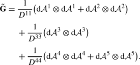
The well-defined metric tensor on the quotient is thereby parameterized by the values of D ¹¹,D ³³ and D ⁴⁴, and we write the metric as a tensor product of left-invariant co-vectors:

The metric tensor on the quotient ℝ³⋊S ² is thereby given by

(36)

where vector fields are described by the differential operators on C ¹(ℝ³×S ²):

(37)

for j=1,2,3, where $R_{\mathbf{e}_{j},h}$ denotes the counter-clockwise rotation around axis e _j by angle h, with e ₁=(1,0,0)^T, e ₂=(0,1,0)^T, e ₃=(0,0,1)^T.

6 Sub-Riemannian Manifolds within SE(3) and Sub-Riemannian Metrics on ℝ³⋊S ²

In the previous section we have classified all legal metric tensors on SE(3) and we have parameterized all legal Riemannian spaces (SE(3),G) by the triplet (D ¹¹,D ³³,D ⁴⁴)∈(ℝ⁺)³. Depending on the choices for D ⁱⁱ, the metric tensor punishes certain tangent directions more than others. Often one would like to impose that flows in our evolutions along specific directions within the tangent space are prohibited (i.e. have infinite cost). See for example Fig. 10, where

• 1. we want to diffuse primarily along $\mathcal{A}_{3}$-direction (and not in the tangent plane spanned by $\{\mathcal{A}_{1},\mathcal {A}_{2}\}$ orthogonal to it) and along the tangent plane spanned by $\{ \mathcal{A}_{4},\mathcal{A}_{5}\}$ (and not in the redundant $\mathcal{A}_{6}$-direction),

• 2. we want to erode primarily in the tangent plane spanned by $\{ \mathcal{A}_{1},\mathcal{A}_{2}\}$ (and not in the $\mathcal {A}_{3}$-direction) and along the tangent plane spanned by $\{\mathcal {A}_{4},\mathcal{A}_{5}\}$ (and not in the redundant $\mathcal {A}_{6}$-direction).

To ensure that certain tangent vector directions are prohibited within the flow of the evolutions U↦Φ _t (U) we need the concept of sub-Riemannian manifolds.

This section studies the differential geometrical consequences of such a prohibition. Together with the preceding group theoretical chapters, it forms the mathematical foundation in the design and analysis of our linear and morphological scale space operators U↦Φ _t (U) which we will introduce in Sect. 7, analyze in Sect. 8, implement in Sect. 9, and apply in Sect. 11. When accepting the formula’s for the Hamiltonian and Lagrangian derived in this section the reader may choose to skip the mathematical details in this section and continue with the next section. In this case, Fig. 10 provides a quick summary of this chapter.

Definition 5

A sub-Riemannian manifold (M,θ ₁,…,θ _n ) with θ _i ∈(T(M))^∗ is a Riemannian manifold (M,G) with the extra constraint that certain subspaces of the tangent space are prohibited, i.e. for all curves γ in (M,θ ₁,…,θ _n ) we have

(38)

The above definition and notation is a suitable simplification of a more accurate⁴ notation and definition of a sub-Riemannian manifold. Curves in M satisfying (38) are called horizontal curves.

Next we consider two specific sub-Riemannian manifolds of $(\mathrm{SE}(3),\tilde{\mathbf{G}})$, that we need when defining respectively linear scale spaces and morphological scale spaces. In both examples we ensure that the available tangent vectors together with their commutators fill the full tangent space T(SE(3)), so that every pair of points in SE(3) can be connected by a horizontal curve.

6.1 The Sub-Riemannian Manifold for Hypo-Elliptic Diffusion

Curves in the sub-Riemannian manifold

are curves $\tilde{\gamma}:[0,L] \to \mathrm{SE}(3)$ such that

(39)

for all s∈[0,L]. Curves satisfying Eq. (39) are called horizontal curves in SE(3) and their tangent vectors are given by

where we use spatial arc length parametrization and short notation

for all s∈[0,L] and i∈{1,…,6}. Such a horizontal curve in SE(3) relates to a horizontal curve in ℝ³⋊S ² via

and we have depicted such a horizontal curve ℝ³⋊S ² in Fig. 10.

Theorem 5

For a horizontal curve s↦γ(s)=(x(s),n(s))∈ℝ³⋊S ² parameterized by spatial arc length one has

where ⁵

is the curvature of the spatial part of the curve. The normal N and binormal B of the spatial part s↦x(s) of a horizontal curve are given by

Proof

Recall from Eq. (30) that $\mathcal{A}_{3}$ is aligned with $\tilde{\mathbf{n}}(\check{\beta },\check{\gamma})$, Eq. (17). Furthermore for spatial arc length parametrization one has $\|\dot{\mathbf{x}}(s)\|= \dot{\gamma}^{3}(s)=1$, since in the sub-Riemannian manifold we have $\dot{\gamma}^{1}=\dot{\gamma}^{2}=0$. W.r.t. the remainder we note that⁶

(40)

where $c^{k}_{ij}$ denote the structure constant of the Lie-algebra. Differentiation of $\dot{\mathbf{x}}(s)= \mathcal{A}_{3}$ (where one applies the product rule and Eq. (40)) produces the required results. □

In previous work [36] we have shown that linear left-invariant diffusion in the group takes place along exponential curves.⁷ When restricting to horizontal diffusion we diffuse locally only along horizontal exponential curves (i.e. along $s \mapsto e^{s (c^{3}A_{3} + c^{4}A_{4} +c^{5}A_{5})}$). So we need this sub-Riemannian manifold $(\mathrm{SE}(3), \mathrm{d}\mathcal {A}^{1}, \mathrm{d}\mathcal{A}^{2}, \mathrm{d}\mathcal{A}^{6})$ for linear horizontal diffusion on ℝ³⋊S ².

The only legal metric tensors on this sub-Riemannian manifold are given by

(41)

The corresponding metric distance on this sub-Riemannian manifold is given by

(42)

with s the spatial arc length parameter and with

Theorem 6

The problem (42) is well-defined for $g_{2}^{-1}g_{1}$ close enough ⁸ to e. The equivalent problem on ℝ³⋊S ² (or rather ℝ³) is:

(43)

where s, L>0, and κ(s) are respectively spatial arc length, total length, and curvature of the spatial part of the curve.

Proof

The metric tensor is left-invariant so that . Now if $g_{2}^{-1}g_{1} \in \mathrm{SE}(3)$ is within the range of the exponential map of the corresponding geometric control problem with particles in SE(3) that move forwardly (i.e. $\dot{x}(s)=+\mathcal{A}_{3}$) along horizontal curves one does not cross cusps [14], similar to the (SE(2),−sinθdx+cosθdy)-case [15]. In such a case it follows that every stationary curve (satisfying the Euler-Lagrange equations on the sub-Riemannian manifold) is a global optimizer. These Euler-Lagrange equations can be found by the Pontryagin maximum principle [4] or by Marsden-Weinstein reduction [16] as we did in [37, Appendix G]. For a visualization and characterization of this exponential map in respectively SE(2) and SE(3) and further details see [15, 44]. The equivalence now directly follows from the identities in Theorem 5 (where the distance is independent of the choice of R _n satisfying Eq. (9)). □

These sub-Riemannian geodesics have as a natural counter-part the elastica curves, where in stead of $\int\sqrt{\|\boldsymbol{\kappa }(s)\|^{2} + \beta^{2}} \mathrm{d}s$ one minimizes the elastica functional ∫∥κ(s)∥²+β ²ds, cf. [38, 59, 72]. The advantage of elastica is that they do not involve cusps, so one does not have to constrain the end-points. Their disadvantage is the vast involvement of special functions and their loss of both global and local optimality, which is fully analyzed for the 2D-case in [72]. See Fig. 11 for an example of geodesic and an elastica and an illustration of the cusp-problem as reported by Boscain and Rossi [14]. For more details see [15, 37, 44].

Fig. 11

Top: Illustration of a 3D-elastica and a 3D-sub-Riemannian geodesic in $(\mathrm{SE}(3), \mathrm{d}\mathcal{A}^{1},\mathrm{d}\mathcal{A}^{2}, \mathrm{d}\mathcal{A}^{6})$, for β=0.1 and depicted for −4≤x,y,z≤4. Arrows indicate the Frenet frame. Bottom left: the boundary conditions for the elastica would yield cusps geodesics. If it is cheaper to set the car in reverse to reach the final destination a smooth minimizer does not exist [14]. Bottom right: In black the planar boundary conditions for which the sub-Riemannian geodesics do not suffer from cusps (for β=1) Eq. (43) has a unique smooth minimizer), for details see [15]

If initial point (x ₀,n ₀)=(x(0),n(0)) and endpoint (x ₁,n ₁)=(x(L),n(L)) are chosen such that

the sub-Riemannian distance on ℝ³⋊S ² given by Eq. (43) is equivalent to the sub-Riemannian distance on $(\mathrm{SE}(2), -\sin\tilde{\theta} \mathrm{d} \tilde{x} +\cos\tilde {\theta} \mathrm{d}\tilde{y})$ that has been studied in full detail by Sachkov and Moiseev [70, 71]. See Fig. 12(top left) for the convention of the $(\tilde{x},\tilde{y})$-coordinate system.

Fig. 12

Top left, if (x ₁−x ₀)×n ₀≡(x ₁−x ₀)×n ₁ then Eq. (43) is equivalent to the sub-Riemannian distance on $(\mathrm{SE}(2), -\sin\tilde{\theta} \mathrm{d} \tilde{x} +\cos\tilde{\theta } \mathrm{d}\tilde{y})$. Right: full field of reachable angles. Bottom left, the set of end-points in SE(2) where a global minimizer exists is an unbounded orientable volume with the cusp-surface as boundary

In Fig. 8 we have depicted such minimizing curves and in Fig. 12 we have plotted the cones of reachable angles (which is precisely the set of end-points in SE(2)≡ℝ²⋊S ¹ where the sub-Riemannian problem has a (global) minimizer). In orientation space this reachable area is a non-compact volume bounded by the cusp-surface (where geodesics arise with infinite curvature, which correspond to the boundaries of the hyperbolic phase portrait in [33, Appendix A]). For more details and formal proofs see [14, 15, 44].

6.2 The Sub-Riemannian Manifold for Erosion

Curves in the sub-Riemannian manifold

embedded in the Riemannian manifold

are curves $\tilde{\gamma}:[0,1] \to \mathrm{SE}(3)$ such that

(44)

for all s∈[0,L]. These horizontal curves satisfy

where the spherical part n(s) is not to be mistaken with the normal N(s) to the spatial part of the curve. More precisely,

Theorem 7

Along the spatial part of a horizontal curve $\tilde{\gamma}$ in $(\mathrm{SE}(3), \mathrm{d}\mathcal{A}^{3}, \mathrm{d}\mathcal{A}^{6})$ we have the following Frenet frame

(45)

with curvature magnitude

where we differentiate w.r.t. to spatial arc length.

Proof

In the sub-Riemannian manifold $(\mathrm{SE}(3), \mathrm{d}\mathcal{A}^{3}, \mathrm{d}\mathcal{A}^{6})$ we have $\langle \mathrm{d}\mathcal{A}^{3}\vert _{\tilde{\gamma}}, \dot{\tilde {\gamma}}\rangle=0$ for horizontal curves $\dot{\tilde{\gamma}}=(\dot{\mathbf{x}},\dot {R}) \in \mathrm{SE}(3)$. Thereby $\mathbf{T}=\mathbf{x}=\dot{\tilde{\gamma }}^{1} \mathcal{A}_{1} + \dot{\tilde{\gamma}}^{2} \mathcal {A}_{2}$, and deriving this expression and using Eq. (40) and B=T×N yields the remaining results. □

Corollary 1

In the special case

• $\dot{\tilde{\gamma}}^{i}=c^{i}$ are constant, we have the exponential curves

  

  with $A_{i}= \mathcal{A}_{i}\vert _{e}$ in which case we have |c ¹|²+|c ²|²=1 and (provided that |c ² c ⁴−c ¹ c ⁵|≠0)

  

  with $\varepsilon=\operatorname{sign}(c^{2}c^{4}-c^{1}c^{5})$. The curvature and torsion magnitude are:

  

  as in [36, Theorem 3].

• $\dot{\tilde{\gamma}}^{2}\dot{\tilde{\gamma}}^{4} - \dot {\tilde{\gamma}}^{1}\dot{\tilde{\gamma}}^{5}=0$, we have $|\dot {\tilde{\gamma}}^{1}|^{2}+|\dot{\tilde{\gamma}}^{2}|^{2}=1$ and

  

We will employ these metric tensors in Hamilton-Jacobi-Belmann equations for morphological scale spaces. In particular for erosions. We want to erode towards the fibers both spatially and angularly, i.e. we need to erode isotropically inwards in the gray planes depicted in Fig. 10.

On $(\mathrm{SE}(3), \mathrm{d}\mathcal{A}^{3}, \mathrm{d}\mathcal{A}^{6})$ we consider the sub-Riemannian distance

(46)

Remark

Because of the isotropy in the plane spanned by $\{\mathcal {A}_{1},\mathcal{A}_{2}\}$ one expects a relation between the Sub-Riemannian metric on $(\mathrm{SE}(3),\mathrm{d}\mathcal {A}^{1},\mathrm{d}\mathcal{A}^{2},\mathrm{d}\mathcal{A}^{6})$ in Eq. (43) and the sub-Riemannian metric δ on $(\mathrm{SE}(3),\mathrm{d}\mathcal{A}^{3},\mathrm{d}\mathcal{A}^{6})$.

Remark

In our sub-Riemannian metric definitions (Eq. (46) and Eq. (42)) we always impose $\langle \mathrm{d}\mathcal{A}^{6}\vert _{\gamma}, \dot{\gamma}\rangle=0$ to avoid⁹ artificial curvature and torsion in the spatial part of the geodesics, for details see cf. [37, Fig. 22].

6.3 Hamiltonians on $(\mathrm{SE} (3),\mathrm{d}\mathcal{A}^{3},\mathrm{d}\mathcal{A}^{6})$

Recall, that in the sub-Riemannian manifold $(\mathrm{SE}(3),\mathrm{d}\mathcal{A}^{1}, \mathrm{d}\mathcal{A}^{2}, \mathrm{d}\mathcal{A}^{6})$ we considered elastica besides the geodesics. We obtained the elastica functional by squaring the integrand while parameterizing by spatial arc length. In $(\mathrm{SE}(3),\mathrm{d}\mathcal {A}^{3},\mathrm{d}\mathcal{A}^{6})$ we do a similar thing, that is we consider powers of the integrands while parameterizing by spatial arc length s∈[0,L]:

(47)

with $\eta\geq\frac{1}{2}$ and $\dot{\gamma}^{i}(s)=\langle \mathrm{d}\mathcal{A}^{i}\vert _{\gamma(s)}, \dot{\gamma }(s)\rangle$. Note that the metric-integrand relates to the Lagrangian via

(48)

The Lagrangian can also be parameterized by the arc length parameter, say p, in the sub-Riemannian manifold, since by Eq. (48) we have

with L the spatial length and t the sub-Riemannian length of the curve where we note that

(49)

Now that we have introduced a Lagrangian on $(\mathrm{SE}(3),\mathrm{d}\mathcal {A}^{1}, \mathrm{d}\mathcal{A}^{2},\mathrm{d}\mathcal{A}^{6})$ we construct the Hamiltonian by means of the Fenchel transform on the Lie-algebra of left-invariant vector fields $\mathcal{L}(\mathrm{SE}(3))$. This construction is a generalization of the relation between Lagrangian and Hamiltonian on ℝⁿ, see [39, Chap. 3.2.2]. In the subsequent section, the Hamiltonian will serve in the generator of morphological scale spaces, where we will generalize morphological scale spaces on ℝⁿ to morphological scale spaces on ℝ³⋊S ².

Definition 6

Let X be a normed space with dual space X ^∗, and let L:X→ℝ∪{∞} be a real-valued function on X, then the Legendre-Fenchel transform on X is given by

where 〈x,y〉=x(y) and x∈X ^∗.

In case X=ℝⁿ, $L(\dot{\mathbf{x}})= \frac{2\eta -1}{2\eta} \|\dot{\mathbf{x}}(s)\|^{\frac{2\eta}{2\eta-1}}$ one gets

In case $X=\mathcal{L}(\mathrm{SE}(3))$ and $L=\mathcal{L}_{\eta}$ we get

(50)

with l:ℝ⁶→ℝ⁺ given by

Theorem 8

The Hamiltonian associated to the Lagrangian (47) is given by

(51)

for all $\mathbf{p}=\sum_{i=1}^{6} p_{i}\mathrm{d}\mathcal {A}^{i} \in(\mathcal{L}(\mathrm{SE}(3)))^{*}$.

Proof

The first identity follows by application of the Pontryagin Maximum Principle [4, 64] to the sub-Riemannian geodesic problem given in Eq. (46) on $(\mathrm{SE}(3),\mathrm{d}\mathcal{A}^{1},\mathrm{d}\mathcal{A}^{2}, \mathrm{d}\mathcal {A}^{6})$. The second identity follows from Eq. (50). □

7 Left-Invariant Scale Spaces on ℝ³⋊S ²

In this section we consider two special cases of evolutions (enhancement) on DW-MRI. In both cases (y,n,t)↦(Φ _t (U))(y,n) is the solution of a PDE system (evolution) defined on (ℝ³⋊S ²)×ℝ⁺ with initial condition Φ ₀(U)=U. For smoothing and fiber propagation in the DW-MRI data U:ℝ³⋊S ²→ℝ⁺ we consider linear scale spaces on ℝ³⋊S ², whereas for well-posed sharpening we consider morphological scale spaces (erosions) on ℝ³⋊S ². For the sake of sober notation we write W(y,n,t):=(Φ _t (U))(y,n) for all t≥0.

7.1 Linear Scale Spaces on ℝ³⋊S ²

The spherical and the spatial Laplacian can be expressed in terms of the left-invariant vector fields:

(52)

where we restrict the rotation generators to the space $\tilde{\mathbb {L}}_{2}(\mathrm{SE}(3)) \subset\mathbb{L}_{2}(\mathrm{SE}(3))$, Eq. (13).

These Laplacians generate diffusion over S ² and ℝ³ separately and are thereby likely to destroy the fiber structure in DW-MRI, recall Fig. 7. Recall our result on legal operators, Theorem 4 and recall Definition 2. From Theorem 4, Eq. (52) and $\mathcal{A}_{6}\vert _{\tilde{\mathbb{L}}_{2}(\mathrm{SE}(3))}=0$, we deduce the following result:

Corollary 2

The only legal linear left-invariant convection-diffusion equations on ℝ³⋊S ² are the following scale spaces:

• 1. Angular diffusion generated by $\Delta_{S^{2}}$,

• 2. Spatial diffusion generated by $\Delta_{\mathbb{R}^{3}}$,

• 3. Contour completion generated by $\pm\mathcal{A}_{3}+ D^{44}\Delta_{S^{2}}$,

• 4. Hypo-elliptic contour enhancement generated by $D^{33}(\mathcal {A}_{3})^{2}+ D^{44}\Delta_{S^{2}}$, D ³³,D ⁴⁴>0

• 5. Elliptic contour enhancement generated by $D^{33}(\mathcal{A}_{3})^{2}+ D^{11}(\mathcal{A}_{1}^{2}+\mathcal {A}_{2}^{2})+ D^{44} \Delta_{S^{2}}$, with D ¹¹,D ³³,D ⁴⁴>0.

In the final option we set 0<D ¹¹≪D ³³, as otherwise fibers propagate too much to the side. To this end we note that for D ¹¹≥D ³³ we have

The scale space evolutions for hypo-elliptic linear contour enhancement are given by:

(53)

These equations boil down to hypo-elliptic diffusion and they are forward Kolmogorov equations of Brownian motion on ℝ³⋊S ² [36, Chap. 4.2], generalizing the approach in [2, 10, 23, 32, 34, 62] to 3D. For linear contour completion we have:

(54)

These equations boil down to hypo-elliptic convection-diffusion and are forward Kolmogorov equation for the direction process on ℝ³⋊S ² [36, Chap. 4.2], generalizing the 2D direction process [10, 35, 59] to 3D.

All of these scale spaces U↦W(⋅,t) are linear, left-invariant and correspond to legal scale spaces on SE(3) and as a result (via Theorem 2) they are solved by convolution with their Green’s function, i.e. impulse-response p _t :

with generator $Q^{\mathbf{D},\mathbf{a}}(\underline{\mathcal{A}})$ corresponding to the legal second order differential operator $\tilde{Q}^{\mathbf {D},\mathbf{a}}(\underline{\mathcal{A}})$ given by Eq. (34). More explicitly formulated; operator

(55)

with D ¹¹=D ²², D ⁴⁴=D ⁵⁵ denotes the generator of the linear scale spaces on ℝ³⋊S ², with differential operators $\mathcal{A}_{i}$ on ℝ³×S ² given by Eq. (37).

Next we address the probabilistic interpretation of the left-invariant (legal) linear scale spaces. The density (y,n)↦W(y,n,t) represents the probability density of finding a random orientated particle (Y _t ,N _t ) at position y∈ℝ³ with orientation n at time t>0 given that the initial distribution of random particles is given by (y,n)↦U(y,n). Now in a Markov-process traveling time is memoryless and the only continuous memoryless distribution is the negative exponential distribution ℙ(T=t)=λe ^−λt. When we condition out the traveling time we obtain the resolvent processes

(56)

This resolvent process coincides with Tikhonov-regularization [36, Theorem 2]. It also appears in implicit finite difference implementations of the linear evolutions [26], when setting λ ⁻¹=Δt.

For contour completion the resolvent process is crucial since it integrates the propagation fronts to a smooth integrable density with a singularity at the origin [36]. However, in contrast to the time-dependent process, it does not satisfy the semigroup property (a crucial scale space axiom [30, 85]). We have

(57)

which has the following implications on the underlying independent random variables:

for all t,s>0. However, for resolvents one has

(58)

Thereby, when alternating the resolvent direction processes (e.g. in an implicit finite difference scheme of the time evolutions), the following relevant questions rise:

• What happens from a probabilistic point of view when alternating these resolvent direction processes?

• What happens with the effective probability density and the singularity at the origin?

• Can we still relate the iterated resolvent process to the original process?

We will answer these questions in the probability section, Sect. 10.2.

In our previous work [36] one can find suitable approximations for all the Green’s functions. See Fig. 3 for an overview with comparison to 2D-equivalents of the Green’s functions. Reasonable parameter settings for 2D-contour completion are (λ,D ¹¹)≈(0.1,0.005) and for the 3D fiber completion (λ,D ⁴⁴)≈(0.1,0.005). Reasonable parameter settings for 2D-contour enhancement are (t,D ¹¹,D ²²)≈(1.25,0.04,1), whereas for 3D fiber enhancement are (t,D ³³,D ⁴⁴)≈(1.25,1,0.04). The analogy in parameter-settings comes from the fact that 3D-completion and enhancement kernels can be approximated by direct products of their 2D-counterparts [36]. Increase t enlarges the time-dependent kernel. Increase of λ ⁻¹ enlarges the resolvent kernel. By a simple re-scaling argument we can set D ³³=1 in which case the parameter D ⁴⁴ is equal to β in the underlying metric-tensor Eq. (43) and thereby tunes the bending of the fiber-propagation kernel. In [5, 17] the authors put an interesting connection between morphological and linear scale spaces on ℝⁿ via the Cramer transform. The Cramer transform does not generalize easily to SE(3), but nevertheless the analogy and probabilistic interpretations of both type of scale spaces remain.

7.2 Morphological Scale Spaces on ℝ³⋊S ²

Recall from Fig. 10 that erosion should take place simultaneously inward in the spatial tangent plane spanned by $\{\mathcal{A}_{1},\mathcal{A}_{2}\}$ and the spherical tangent plane spanned by $\{\mathcal{A}_{4},\mathcal{A}_{5}\}$. As a result we must consider the underlying sub-Riemannian manifold $(\mathrm{SE}(3),\mathrm{d}\mathcal{A}^{3},\mathrm{d}\mathcal{A}^{6})$ equipped with metric tensor $\tilde{\mathbf{G}}$ given by Eq. (35) with D ³³→∞. According to Theorem 4 this metric tensor on the sub-Riemannian manifold $(\mathbb{R}^{3}\rtimes S^{2},\mathrm{d}\mathcal{A}^{3})$ is legal.

Let $\frac{1}{2}\leq\eta<\infty$ and recall the Hamiltonian given by Eq. (51). Then the corresponding Hamilton-Jacobi-Bellman (HJB) equations provide the morphological scale space equations for erosion (− case) on ℝ³⋊S ²:

(59)

where the left-invariant gradient of the corresponding function $\tilde {W}(\cdot,t)$ on SE(3) (recall Eq. (11)) is given by

(60)

Remark

For η→∞ we naturally arrive at the time-independent HJB-equation (Eikonal Eq.)

where the Hamiltonian $\mathcal{H}_{\infty}$ relates to the homogeneous Lagrangian

One solution is W(y,n)=δ((0,I),(y,R _n )) where δ denotes the sub-Riemannian distance on $(\mathrm{SE}(3), \mathrm{d}\mathcal{A}^{3},\mathrm{d}\mathcal{A}^{6})$, cf. Eq. (46).

The HJB-equations on ℝ³⋊S ² have an important geometric property (similar to HJB-equations on ℝⁿ, cf. [60, 74, 81]) as we will show next.

Definition 7

A family $\{\mathcal{S}_{t}\}_{t \in\mathbb{R}^{+}}$ of surfaces

(61)

is geodesically equidistant if

(62)

for all geodesics passing these surfaces transversally with $\tilde{W}(\gamma(t),t)=W_{0}(t)$ that minimize

(63)

The equivalence in Eq. (62) denotes equality up to a monotonic re-parametrization of time.

Theorem 9

A family of surfaces $\mathcal{S}_{t}$ given by Eq. (61) is geodesically equidistant iff W satisfies the HJB-equation (where time may be re-parameterized)

For a proof see Appendix B.

Corollary 3

Iso-contours of solutions of our morphological scale spaces are geodesically equidistant in the underlying sub-Riemannian manifold $(\mathbb{R}^{3}\rtimes S^{2},\mathrm{d}\mathcal {A}^{1},\mathrm{d}\mathcal{A}^{2})$.

The morphological scale spaces (59) do not have unique solutions. This is well-known for the special case where one has only angular erosion or only spatial erosion [24, 39]. Based on these works we have the following definition of viscosity solutions on ℝ³⋊S ².

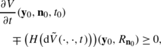
Definition 8

Suppose that the Hamiltonian is convex and H(p)→∞ as p _i →∞, i=1,…5. Then a viscosity solution is a bounded and continuous (not necessarily differentiable) weak solution W:(ℝ³⋊S ²)×ℝ⁺→ℝ of (59) such that

• 1. for any smooth function V:(ℝ³⋊S ²)×ℝ⁺→ℝ such that W−V attains a local maximum at (y ₀,n ₀,t ₀) one has

  

  (64)

• 2. for any smooth function V:(ℝ³⋊S ²)×ℝ⁺→ℝ such that W−V attains a local minimum at (y ₀,n ₀,t ₀) one has

  

  (65)

where $\mathrm{d}\tilde{V}(\cdot,\cdot,t)= \sum_{i=1}^{5}\mathcal {A}_{i}\tilde{V}(\cdot,\cdot,t) \mathrm{d}\mathcal{A}^{i}$ denotes the left-invariant gradient of the corresponding function defined on the group SE(3), related to V(⋅,⋅,t) via Eq. (11), at each time t≥0.

To get some intuition on the concept of viscosity solutions on ℝⁿ we note that the name viscosity solutions refers to the propagation of viscous fluids, where propagation fronts can not propagate through each other, cf. Fig. 13

Fig. 13

Solutions of dilation equations on ℝ^d, d=1,2, that are not viscosity solutions. For d=1 these solutions are highly undesirable as they would produce non-existing structure from a zero initial condition. For d=2 the dilation equation describes the propagation of geodesically equidistant surfaces (isolines of the solution) [81] in ℝ². Suppose we put two morphological deltas then we do want propagation fronts that propagate through each other

According to the following theorem, we have that the unique viscosity solutions of our morphological scale spaces are given by erosions/dilations with the corresponding Green’s functions.

Theorem 10

The viscosity solutions of

(66)

are given by (− case) left-invariant erosion

(67)

and (+ case) left-invariant dilation

(68)

with the corresponding morphological Green’s function. The morphological Green’s functions are given by $-k_{t}^{D^{11} ,D^{44} ,\eta,-}(\mathbf{y},\mathbf{n})= k_{t}^{D^{11} ,D^{44} ,\eta,+}(\mathbf{y},\mathbf{n})$ and

(69)

with spatial arc length s given by $s(\tau):= \int_{0}^{\tau} \|\dot{\mathbf{x}}(\tau)\| \mathrm{d}\tau$, and with ℝ³⋊S ²-“erosion arc length” given by

(70)

The exact erosion/dilation kernels satisfy the semigroup property

(71)

for all t,s>0, where we recall Eq. (25).

Proof

See Appendix A. □

In Eq. (70) we can use any parametrization of a smooth curve τ↦γ(τ) in the sub-Riemannian manifold $(\mathrm{SE}(3), \mathrm{d}\mathcal{A}^{3},\mathrm{d}\mathcal{A}^{6})$. For example if τ=s (spatial arc-length) we find

(72)

with $\dot{\gamma}^{i}(s):=\langle \mathrm{d}\mathcal {A}^{i}\vert _{\gamma(s)}, \dot{\gamma}(s)\rangle$. This yields the following result

Lemma 4

The integral of the morphological Green’s function can also be expressed using integration with respect to s:

(73)

where L denotes the total length of x(⋅) and where the Lagrangian $\mathcal{L}_{\eta}$ is evaluated along the curve

where the components of the tangent vector w.r.t. our moving left-invariant frame of reference are given by

Proof

This follows by the homogeneity of the Lagrangian, the chain law, Eqs. (72) and (49). □

Spatial arc length parametrization of the curves in sub-Riemannian manifolds within SE(d), d=2,3 is often preferable over sub-Riemannian arc length parametrization, as it involves less special functions, cf. [33, Appendix A], [70], and the parametrization breaks down precisely at the cusps (which are exactly the points where both global and local optimality is lost [15]) recall Fig. 11. However, for generalizing the results on viscosity solutions of HJB-equations on ℝ³, [5, 17, 24, 39] to ℝ³⋊S ² the p-parametrization seems to be more suitable.

8 Tangible Approximations of Linear and Morphological Green’s Functions

The derivation of the exact formula for the morphological kernel in Eq. (69) is very complicated: One first would have to derive the curve minimizers via reduction of a complicated Pfaffian system (following a Lagrangian approach similar to the derivation of the sub-Riemannian geodesics in [37, Appendix G], [16], [44]) or the Pontryagin maximum principle (following a Hamiltonian approach [4]). A direct classical variational Lagrangian approach (similar to [59]), without relying on symplectic geometry can also be done. It yields the same curves, but only after highly cumbersome bookkeeping and computations, [44].

On top of that, one has the problem that once the stationary curves are derived by integration of the Lagrangian or Hamiltonian system, one must solve a boundary value problem that involves at least 1 special function (similar to the SE(2)-case [15]) and in order to compute the morphological kernel in Eq. (69) one must resort to a quite involved numerical algorithm [44] for every (y,n)∈ℝ³⋊S ².

A more reasonable, but less accurate, alternative would be to apply an upwind finite difference scheme of (59) that is explained in Sect. 9.3. However, this would require interpolations in the rotated, translated and reflected kernels in Theorem 3. Therefore, if it comes to fast practical kernel implementations (both for the morphological and linear case) and analysis we prefer to use the approximations presented in the next theorem.

Theorem 11

Let $\frac{1}{2}<\eta\leq1$, D ¹¹>0,D ³³>0,D ⁴⁴>0. Then for the morphological erosion (+) and dilation kernel (−) on ℝ³⋊S ² one can use the following asymptotic approximation (for t>0 small)

(74)

with $\mathbf{n}=(\sin\tilde{\beta},-\cos\tilde{\beta} \sin \tilde{\gamma}, \cos\tilde{\beta} \cos\tilde{\gamma})^{T}$, c>0, with $\tilde{\beta} \in(-\frac{\pi}{2},\frac{\pi}{2})$, $\tilde{\gamma} \in(-\frac{\pi}{2} ,\frac{\pi}{2})$. For the Green’s functions of Eq. (53), the heat kernels, we have the approximation

(75)

The functions $c^{i}:=c^{i}(\mathbf{y},\tilde{\alpha}=0,\tilde {\beta},\tilde{\gamma})$ are given by

(76)

with $\tilde{q}=\arcsin\sqrt{\cos^{4}(\tilde{\gamma}/2) \sin^{2}(\tilde{\beta}) + \cos^{2}(\tilde{\beta}/2) \sin^{2}(\tilde{\gamma})}$.

Proof

We apply the theory of weighted sub-coercive operators on Lie groups here [78, Proposition] and/or the general Ball-box theorem [12, 13] that provides a local uniform estimate for sub-Riemannian metrics. For hypo-elliptic diffusion we must consider the sub-Riemannian manifold: $(\mathrm{SE}(3),\mathrm{d}\mathcal{A}^{1},\mathrm{d}\mathcal{A}^{2}, \mathrm{d}\mathcal{A}^{6})$ (recall Fig. 10). This induces the following filtration:

Now there exist Gaussian approximations

(77)

for 0<a ₁≤a ₂ and b ₁≥b ₂>0 for hypo-elliptic Green’s functions $\tilde{P}_{t}^{D^{33},D^{44},D^{55}}$ with respect to the sub-Riemannian metric [78]. Now by the ball-box theorem the sub-Riemannian metric on $(\mathrm{SE}(3), \mathrm{d}\mathcal{A}^{1},\mathrm{d}\mathcal{A}^{2}, \mathrm{d}\mathcal{A}^{6})$ can be estimated by the weighted modulus

(78)

with $A_{i}= \mathcal{A}_{i}\vert _{e}$, c>1, for all g close to e. For the explicit expression of the log-coefficients c ⁱ in terms of our Euler angles (17) see [36, Eq. (76)]. Here we stress that the exponential map exp:T _e (SE(3))→SE(3) is surjective. In case of the nilpotent Heisenberg approximation of the Euclidean motion one can get a grip on the constant c>1 (which is not that far from 1 see [32, 36]). The precise value of c>1 is not crucial for this theorem as it can be taken into account by a rescaling of time t↦c ⁻¹ t.

Now the sub-Riemannian balls

in $(\mathrm{SE}(3),\mathrm{d}\mathcal{A}^{1},\mathrm{d}\mathcal{A}^{2},\mathrm{d}\mathcal{A}^{6})$ are similar to their ball-box estimates non-smooth, whereas the heat-kernels are smooth due to the Hormander Theorem [49]. Therefore we use the locally equivalent smooth modulus

(79)

Now the result (75) follows by Eq. (78), (77), (79) and rescaling of the Lie-algebra generators.

Note that a subtlety arises here: the logarithm is well-defined on SE(3) but it is not well-defined on ℝ³⋊S ², it is therefore important that in our approximations one takes a consistent section in the principal fiber bundle (SE(3),ℝ³⋊S ²,{0}⋊SO(2)) with total space SE(3), base manifold ℝ³⋊S ² and structure group {0}⋊SO(2) acting via the right action R _h g=gh and with projection g↦[g]=g({0}⋊SO(2)). Since we identified (0,e _z ) with the unity e=(0,I)∈SE(3) we must set $\tilde{\alpha}=0$ in all Lie-algebra coefficients c ⁱ, since in our approximation we should stick to the consistent cross section, cf. [36, Chap. 7].

For the result (74) on approximations of morphological Green’s functions, we first consider the case η→∞, D ¹¹=D ⁴⁴=1. In this case the Lagrangian is homogeneous and we consider the sub-Riemannian distance δ given by Eq. (46) defined on the sub-Riemannian manifold $(\mathrm{SE}(3),\mathrm{d}\mathcal{A}^{3},\mathrm{d}\mathcal {A}^{6})$:

(80)

Note that for erosions we need a different sub-Riemannian manifold than for diffusion, recall Fig. 10. Now again by the Ball-box theorem and the equivalent smooth modulus trick δ is locally equivalent to the following weighted modulus on the Lie-algebra

The result for $\frac{1}{2}<\eta\leq1$ follows by the Fenchel-transform on $\mathcal{L}(\mathrm{SE}(3))$ and Theorem 8. The result (74) for general g _ii =(D _ii )⁻¹>0 follows by re-scaling of the Lie-algebra basis. Finally, the positive Green’s function for erosion is minus the negative Green’s function for dilation. □

Remarks

• Erosion ball in SE(3) around the unity, i.e. the ball

  

  with r>0 small, are equivalent to balls

  

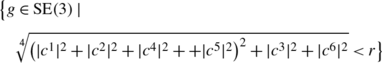
  induced by weighted modulus on the Lie-algebra of SE(3) (with c ⁱ=c ⁱ(g) the logarithm coefficients). This underlies our asymptotical formula (74). This gives us a simple analytic approximation formula for the balls in the sub-Riemannian manifold $(\mathrm{SE}(3),\mathrm{d}\mathcal{A}^{3}, \mathrm{d}\mathcal{A}^{6})$, without determining the minimizing curves (i.e. geodesics) in Eq. (46).

• Next we provide some background in the weighting in the weighted modulus. In general it is not possible to connect any two points, say e and g, via a horizontal exponential curve. This means that not every element $(\mathbf{y},R_{\mathbf {e}_{z},\gamma}R_{\mathbf{e}_{y},\beta}) \in \mathrm{SE}(3)$ is reached by an exponential curve of the type $h \mapsto e^{h \sum_{i\in\{1,2,4,5\}} c^{i}A_{i}}$ starting from e. In fact, by the Campbell-Baker-Hausdorff (CBH) formula and the commutator table above Eq. (33) one has

  

  (81)

  which explains the different weighting of the missing Lie-algebra directions.

• From a practical point of view one typically wants to erode in the sub-Riemannian manifold $(\mathrm{SE}(3),\mathrm{d}\mathcal{A}^{3}, \mathrm{d}\mathcal{A}^{6})$ and to dilate in sub-Riemannian manifold $(\mathrm{SE}(3),\mathrm{d}\mathcal{A}^{1}, \mathrm{d}\mathcal{A}^{2}, \mathrm{d}\mathcal{A}^{6})$. In this case the erosion process sharpens the fibers, whereas the latter process would dilations of fibers (rather than shortening them). One can combine these processes in a single erosion-dilation process on SE(3).

• The underlying idea in the logarithmic approximation within a (sub-)Riemannian manifold in SE(3) is that one keeps the non-zero coefficients $\dot{\gamma}^{i}$ constant. This is equivalent to considering auto-parallels of the Cartan connection on the underlying principal fiber bundle [33, 36]. The auto-parallels of the Cartan connection are the (horizontal) exponential curves, which due to the torsion of the Cartan connection do not coincide with the (sub)-Riemannian geodesics. However, due to the commutator relations and the CBH-formula this torsion kicks in as a second order effect and locally we can approximate with an aligned exponential curve.¹⁰

9 Implementation of (Morphological) Scale Spaces on ℝ³⋊S ²

We distinguish between two implementations for morphological scale spaces:

• 1. Erosion via convolutions with the tangible approximations of the morphological Green’s functions derived in the previous section.

• 2. Left-invariant finite-difference upwind schemes.

As a result of the non-commutative nature of SE(3), the space ℝ³⋊S ² of positions and orientations is coupled, recall Figs. 8 and 10. Thereby both implementations are not separable in a spatial and angular part. In fact, this only occurs in the (less-interesting) case where D ¹¹=D ²²=0 or D ⁴⁴=D ⁵⁵=0, in which case we respectively restrict ourselves to angular erosion and spatial erosion:

• Angular erosion (i.e. erosion on each glyph): In case D ¹¹=D ²²=0 and D ⁴⁴=D ⁵⁵>0 the erosion kernels are given by

  

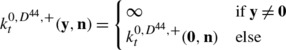
  such that the angular erosions are given by

  

  (82)

• Spatial erosion (i.e. the same erosion for all orientations): If D ¹¹=D ²²>0, and D ⁴⁴=D ⁵⁵=0 the erosion kernels are

  

  such that the spatial erosions are given by

  

Advantages kernel implementations:

• 1. they allow fast parallel algorithms via look-up tables and precomputed Green’s functions, akin to accelerated implementations [68] of linear ℝ³⋊S ²-convolutions, [36].

• 2. they are unconditionally stable and direct relate to viscosity solutions (Theorem 10).

• 3. they involve less interpolation.

Advantages finite difference schemes:

• 1. they are much more flexible towards data adaptive extensions, cf. [26].

• 2. they use efficient (short) stensils of interpolated finite differences, cf. [26].

• 3. do not involve analytic asymptotical approximations (e.g. no rescaling of time via c>0).

The implementations are complementary; the finite differences can be used for accurate precomputation of the Green’s functions used in the convolution schemes. Both implementations are included in our Mathematica package available (for academic purposes only) at www.bmia.bmt.tue.nl/people/RDuits/DWIpackage/HARDIAlgorithms.zip.

9.1 Geometric Erosion Parameters

The erosions given by Eq. (59) involve four fundamental parameters, t, D ¹¹, D ⁴⁴ and η. However, the erosion equations can be re-scaled such that D ¹¹=1, leaving only 3 degree of freedom.

The fraction D ¹¹/D ⁴⁴ determines the relative strength of angular erosion compared to spatial erosion and this parameter has physical dimension [Length]². After rescaling the underlying sub-Riemannian metric tensor becomes

A large value of D ¹¹/D ⁴⁴ yields a domination of spatial erosion, a small value of D ¹¹/D ⁴⁴ yields a domination of angular erosion. The stopping time parameter t>0 indicates the size of the erosion-kernels. Although not considered here, statistical approaches could be used to estimate a suitable stopping time from a given DW-MRI data-set. To get a visual impression of the typical effect of (D ¹¹/D ⁴⁴,t) on the erosion output, we refer to Fig. 14. The parameter $\eta\in(\frac{1}{2}, 1]$ determines the power of the Hamiltonian. For $\eta\downarrow\frac{1}{2}$ we get a homogeneous Hamiltonian and a flat morphological approximation kernel (take $\eta\downarrow \frac{1}{2}$ in Theorem 11):

(83)

The typical effect of including η is depicted in Fig. 15 where we applied angular erosion only (i.e. D ¹¹=∞), see Eq. (82). Due to the fact that the approximation of the erosion kernel in Theorem 11 is a quadratic form on the logarithmic coefficients that depend on goniometric functions of the angles $\tilde{\beta}$ and $\tilde{\gamma}$ along the cross-section $\tilde{\alpha}=0$ the erosion kernel is not very suited for a glyph-field visualization. To get an impression of the shape of the balls in $(\mathrm{SE}(3),\mathrm{d}\mathcal{A}^{3},\mathrm{d}\mathcal{A}^{6})$ it is more intuitive to plot the corresponding Gaussian estimation of the hypo-elliptic diffusion kernels on $(\mathrm{SE}(3),\mathrm{d}\mathcal{A}^{3},\mathrm{d}\mathcal{A}^{6})$, see Fig. 16. These Gaussian estimates are given by

(84)

Fig. 14

Top row: output angular erosion on a single glyph with crossings for several parameter settings. Middle row: input and output of simultaneous spatial and angular erosion (i.e. ℝ³⋊S ²-erosion), where angular erosion dominates t=3,D ⁴⁴/D ¹¹=2. Bottom row: input and output of ℝ³⋊S ²-erosion, where angular spatial erosion dominates t=2,D ⁴⁴/D ¹¹=1/3

Fig. 15

The effect of $\eta\in[\frac{1}{2},1]$ on angular erosion Eq. (59), with D ⁴⁴=0.4, D ¹¹=0 and t=0.4. Left: original glyph, right eroded glyphs (normalized)

Fig. 16

Top, left; approximation erosion kernel (D ¹¹=1,D ⁴⁴=0.04,t=1.2) on $(\mathrm{SE}(3),\mathrm{d}\mathcal{A}^{3},\mathrm{d}\mathcal{A}^{6})$ where we clipped function values to 2. The holes in the spheres describe the relevant part of the erosion kernels. Top, right; Gaussian approximations of the hypo-elliptic heat-kernels on $(\mathrm{SE}(3),\mathrm{d}\mathcal{A}^{3},\mathrm{d}\mathcal{A}^{6})$. Bottom, left; Gaussian approximations of the hypo-elliptic heat-kernels on $(\mathrm{SE}(3),\mathrm{d}\mathcal{A}^{1}, \mathrm{d}\mathcal{A}^{2},\mathrm{d}\mathcal{A}^{6})$ for (par’s:D ³³=1, D ⁴⁴=0.04, t=0.8), middle; output convolution algorithm (cf. Lemma 1) of the kernel on the left with itself, right; Gaussian approximations of the hypo-elliptic heat-kernels on $(\mathrm{SE}(3),\mathrm{d}\mathcal{A}^{1},\mathrm{d}\mathcal{A}^{2}, \mathrm{d}\mathcal{A}^{6})$ for (D ³³=1, D ⁴⁴=0.04, t=1.6). The similarity shows us that the coarsely sampled (on a 5×5×5×162-grid) Gaussian approximations still nearly satisfy the semi-group property (57)

9.2 Kernel Implementations

Kernel implementation for dilations/erosions on ℝ³⋊S ² are entirely analogous to kernel implementations of linear diffusion on ℝ³⋊S ², except for a change in the algebra. For dilations one uses the (max,+)-algebra whereas with diffusion one uses the (+,⋅)-algebra. For erosions one uses the (min,+)-algebra. This is directly observed by comparing Lemmas 1 and 5. We use the fast tangible morphological kernel approximations in Theorem 11.

9.3 Finite Difference Implementations

Similar to our finite difference schemes for left-invariant diffusions [26, 36] we use a Euler-forward first order time integration scheme. However, for morphological scale spaces we use a so-called upwind-scheme, where the sign of the central difference determines whether a forward or backward difference is taken.

(85)

with spatial step-size h>0 and angular step-size h _a >0, and with a ^±,k given by

For further details on implementation of the left-invariant finite differences on ℝ³⋊S ² and the involved interpolation we refer to [26].

9.4 Adaptive Morphological Scale Spaces

It is very interesting to consider adaptive dilations on ℝ³⋊S ², in a similar way as with adaptive diffusions [42]. This would generalize the efficient dilation [19, 63] of DTI-tensors to (diffused) high angular resolution DW-MRI-images defined on ℝ³⋊S ². This could be done by multiplying the left-invariant gradient $\mathrm{d}\tilde{W}$, Eq. (60), with a data adaptive positive definite help-matrix in SO(3)⊕SO(3), before substituting it into the Hamiltonian in Eq. (59). Here the idea of gauging the local reference frame to include curvature adaptation and deviation for horizontality based on locally optimal exponential-curves in SE(2) [33, Chap. 3.4], could be generalized to SE(3). However, adaptive dilations and erosions on the full space ℝ³⋊S ² are beyond the scope of this article.

Here we just provide a simple mechanism for data-adaptive angular erosion and dilation as a first step towards adaptive erosions on ℝ³⋊S ².

9.5 Data Adaptive Erosion and Dilation on S ²

In the erosion evolution (59) one can include adaptivity by making D ⁴⁴ dependent on the local Laplace-Beltrami-operator

with ϕ a monotonic, odd function and

The intuitive idea here is to create a soft transition between dilation and erosion on a glyph x+μ{U(x,x)n∣n∈S ²}. In the vicinity of a spherical maximum the $\Delta_{S^{2}}$ is positive, whereas in the vicinity of a spherical minimum the $\Delta_{S^{2}}$ is negative. The constant c determines where the transition should take place. See Fig. 17 where we set $\phi(x)=D^{44} x^{\frac{1}{3}}$ with varying c (erosion near maxima) and Fig. 18 where we compare the case $\phi(x)= D^{44} x^{\frac{1}{3}}$ to the case $\phi(x)=-D^{44} x^{\frac {1}{3}}$ (erosion near minima).

Fig. 17

From left to right, input glyph at say y=0. Sample points where $\Delta_{S^{2}}U(\mathbf{0},\mathbf{n})<0$ resp. ≥0 are respectively indicated in red and blue. Linearly eroded glyph (D ⁴⁴=0.45, t=0.5, η=1, Δt=0.01), adaptive eroded glyph (D ⁴⁴=0.45, t=0.5, η=1, $\phi(x)=D^{44} x^{\frac {1}{3}}$) (Color figure online)

Fig. 18

Left: input, middle: adaptive erosion near maxima, right: adaptive erosion near minima. (D ⁴⁴=0.4, t=1, η=1, $\phi (x)=\pm D^{44} x^{\frac{1}{3}}$, Δt=0.01)

10 The Underlying Probability Theory

In this section we address the underlying probability of scale spaces on ℝ³⋊S ². We first consider probability theory underlying linear scale spaces on ℝ³⋊S ², and then a probabilistic interpretation of morphological scale spaces on ℝ³⋊S ².

10.1 Brownian Motions on ℝ³⋊S ²

Next we formulate a left-invariant discrete Brownian motion on SE(3). The left-invariant vector fields $\{\mathcal{A}_{1},\ldots,\mathcal {A}_{6}\}$ form a moving frame of reference to the group. There are two ways of considering vector fields. Either one considers them as differential operators on smooth locally defined functions, or one considers them as tangent vectors to equivalent classes of curves. These two viewpoints are equivalent, for formal proof see [9, Prop. 2.4]. So far we have used the first way of considering vector fields, but in this section we prefer to use the second way. We will write {e ₁(g),…,e ₆(g)} for the left-invariant vector fields (as tangent vectors to equivalence classes of curves) rather than the differential operators $\{ .\mathcal{A}_{1}\vert _{g},\ldots, \mathcal{A}_{6}\vert _{g}\}$. We obtain the tangent vector e _i from $\mathcal{A}_{i}$ by replacing

(86)

where we identified SO(3) with a ball with radius 2π whose outer-sphere is identified with the origin, using Euler angles $R_{\mathbf{e}_{z},\gamma} R_{\mathbf {e}_{y},\beta} R_{\mathbf{e}_{z},\alpha} \leftrightarrow\alpha \mathbf{n}(\beta,\gamma) \in B_{\mathbf{0},2\pi}$. Next we formulate left-invariant discrete random walks on SE(3) expressed in the moving frame of reference $\{\mathbf{e}_{i}\}_{i=1}^{6}$ given by (86):

for all n=0,…,N−1, with random variable (Y ₀,n ₀) is distributed by U ^D, where U ^D are the discretely sampled DW-MRI data and where the random variables (Y _n ,N _n ) are recursively determined using the independently normally distributed random variables $\{\varepsilon_{i,n+1}\}_{i=1,\ldots,5}^{n=1,\ldots, N-1}$, $\varepsilon_{i,n+1} \sim\mathcal{N}(0,1)$ and where the stepsize equals $\Delta s=\frac{s}{N}$ and where $\mathbf{a}:=\sum_{i=1}^{5} a_{i}\mathbf{e}_{i}$ denotes an apriori spatial velocity vector having constant coefficients a _i with respect to the moving frame of reference $\{\mathbf{e}_{i}\}_{i=1}^{5}$ (just like in (34)). Now if we apply recursion and let N→∞ we get the following continuous Brownian motion processes on SE(3):

(87)

with $\varepsilon_{i} \sim\mathcal{N}(0,1)$ and (X(0),N(0))∼U and where $\sigma= \sqrt{2D} \in\mathbb{R}^{6\times6}$, σ>0.

Now if we set $U=\delta_{\mathbf{0},\mathbf{e}_{z}}$ (i.e. at t=0, we have only one orientated particle located at (0,e _z )) then suitable averaging of infinitely many random walks of this process yields the transition probability density

with evolution generator given by Eq. (55).This probability density is the Green’s function of left-invariant evolution equations on ℝ³⋊S ²

that are the Forward Kolmogorov equation of the general stochastic process (87). This follows by Ito-calculus and in particular Ito’s formula for formulas on a stochastic process, for details see [22, Chap. 4.5, Chap. 8], [7, Appendix A] where one should consistently replace the left-invariant vector fields of respectively SE(2) and ℝⁿ by the left-invariant vector fields on SE(3).

In particular we have the direction process for contour completion in ℝ³⋊S ² where

(88)

with Fokker-Planck equation (54) and the (horizontal) Brownian motion for contour-enhancement in ℝ³⋊S ² where

(89)

with Fokker-Planck equation (53), for D ₁₁=0.

Instead of considering the probability density W(y,n,t) of finding a random walker at time t at position y and orientation n given that it started from the initial distribution U, one can also consider the probability density P _λ (y,n) of finding a random walker at position y with orientation n given that it started from the initial distribution U regardless its traveling time T∼NE(λ). Then by Eq. (7.1) we must apply the resolvent operator to the initial condition:

(90)

The (resolvent) Green’s functions and the corresponding stochastic processes for contour-completion and contour enhancement are illustrated in Fig. 3.

10.2 The Time Integrated Direction Process

In the previous work [36] the resolvent processes of contour enhancement are studied and according to [36, Theorem 2] they are related to Tikhonov regularization on ℝ³⋊S ². The corresponding resolvent kernels do not satisfy the semi-group property (cf. Eq. (58)) and the question rises what happens when alternating Tikhonov regularization steps. The same question is particularly important with contour completion, where the resolvent processes integrate the moving propagation fronts of the convection-diffusions.

The solution $P_{\lambda}(\mathbf{y},\mathbf{n})=(R_{\lambda }^{\mathbf{D},\mathbf{a}}*_{\mathbb{R}^{3} \rtimes S^{2}}U)(\mathbf {y},\mathbf{n})$ of (90) represents the probability density of finding a random walker at position y with orientation n given that it started from the initial distribution U regardless its traveling time. In a Markov process, traveling time is memoryless and thereby negatively exponentially distributed T∼NE(λ).

There is however, a practical drawback induced by this memoryless property: Both the time-integrated resolvent kernel of the direction process and the time-integrated resolvent kernel of the enhancement process suffer from a serious singularity at the unity element. For example, in [37, Appendix D] we derived an asymptotical formula for the resolvent contour enhancement kernel, from which we deduce

where $|g|_{D^{33},D^{44}}=|(\mathbf{y},R_{\mathbf {n}})|_{D^{33},D^{44}}$ is the weighted modulus on SE(3) given by

with c ⁱ the logarithmic coefficients given by (76), recall Theorem 11. Consequently, the kernels are in practice too much concentrated around the singularity for visually appealing results. Therefore, we introduce a k-fold iterative approach and address the three related questions raised at the end of Sect. 7.1.

10.3 The Iteration of Resolvent Operators

The sum $T=\sum_{i=1}^{k} T_{i}$ of k independent negatively exponentially distributed random variables T _i ∼NE(λ) is Gamma distributed:

with temporal convolutions given by $(f*_{\mathbb{R}^{+}}g)(t)= \int_{0}^{t}f(t-\tau) g(\tau) \mathrm{d}\tau$. Application of the Laplace transform $\mathcal{L}$, given by $\mathcal{L}f(\lambda)=\int_{0}^{\infty}f(t)e^{-t \lambda} \mathrm{d}t$ yields $\mathcal{L}(f*_{\mathbb{R}^{+}}g)=\mathcal{L}(f) \cdot \mathcal{L}(g)$ and thereby

(91)

Now for the sake of illustration we set k=2 for the moment and we compute the probability density of finding a random walker G _T ∈ℝ³⋊S ² with traveling time T=T ₁+T ₂ at position y with orientation n given that it at t=0 started at (0) with orientation e _z . Basically this means that the path of the random walker has two stages, first one with time T ₁∼NE(λ) and subsequently one with traveling time T ₂∼NE(λ) and we have

(92)

where $*=*_{\mathbb{R}^{3}\rtimes S^{2}}$ denotes convolution on ℝ³⋊S ² as in Theorem 2. By induction this can easily be generalized to the general k-step approach:

An alternative derivation of the result arises by

which only holds in the distributional sense, where with respect to the crucial second equality we recall Eq. (91). We have proved the following result.

Theorem 12

A concatenation of k subsequent and independent time-integrated memoryless stochastic process for contour completion(/enhancement) with expected traveling time λ ⁻¹, corresponds to a time-integrated contour completion(/enhancement) process with a Gamma distributed traveling time

The probability density function (Green’s function) of this stochastic process is given by

Figure 20 shows some experiments of contour completion on an artificial data set containing fibers with a gap we would like to complete, for various parameter settings of (λ,k), where T _i ∼NE(λ) and k denotes the iteration index of the time integrated contour-completion process. In principle this scheme boils down to ℝ³⋊S ²-convolution (applying Lemma 1 and Theorem 2) with the Green’s functions depicted in Fig. 19. For a fair comparison we kept the expected value constant, that is $E(T)=E(T_{1}+\cdots +T_{k})=\frac{k}{\lambda}=4$ in Fig. 19 and $E(T)=E(T_{1}+\cdots +T_{k})=\frac{k}{\lambda}=2$ in Fig. 20, which roughly coincides with half the size of the gap. Note that the results hardly change after two iterations, as the graphs of the scaled Gamma distributions $\varGamma(\cdot ; \frac{k}{2},k)/\varGamma((2(k-1)/k) ; \frac{k}{2},k)$ are similar for k=2,3,4.

Fig. 19

Glyph visualization, recall Definition 1, of the kernels $R_{\lambda,k=2}^{\mathbf{D},\mathbf{a}}:\mathbb {R}^{3}\rtimes S^{2} \to \mathbb{R}^{+}$, with diffusion matrix $\mathbf{D}=\operatorname{diag}\{ 0,0, 0,D^{44},D^{44},0\}$ and convection vector a=(0,0,1,0,0,0), for several parameter-settings (λ,k) for D ⁴⁴=0.005. Kernels are sampled and computed on a spatial 8×8×8-grid and on an a 162-point tessellation of the icosahedron using a left-invariant finite difference scheme, cf. [25, 26]

Fig. 20

Glyph visualization, recall Definition 1, of a left-invariant finite difference scheme, cf. [26], on a 12×12×12-grid and 162-point tessellation of the icosahedron, applied to the input data set, according to our resolvent contour-completion process, ref. Eq. (87), with D ⁴⁴=0.005 and a ³=1, iterated k-times with E(T _i )=λ ⁻¹

We conclude that the k-step approach with k>1 provides much more effective completion of gaps within fibers in ℝ³⋊S ² than the case k=1, as can be observed in Figs. 19 and 20. This mainly due to the fact that the order of the singularity at the origin decreases (it takes 5 steps to get rid of the singularity [37, Chap. 10.1.1, Appendix D]).

10.4 Bellman Processes on ℝ³⋊S ²

In this subsection we present a short overview of cost processes on SE(3). The mapping I↦lim _ε→0log _ϵ I defines a morphism of the (+,⋅)-algebra to the (min,+)-algebra on ℝ⁺ (the co-domain of our DW-MRI images) and it is indeed readily verified that lim _ε→0log _ϵ ϵ ^a⋅ϵ ^b=a+b and lim _ε→0log _ϵ (ϵ ^a+ϵ ^b)=min(a,b). Using this map, various notions of probability calculus can be mapped to their counterparts in optimization problems. Next we mention the following definitions as given by Akian, Quadrat and Viot in [5] adapted to our case.

Definition 9

The decision space is the triplet $(\mathrm{SE}(3), \mathcal {O}(\mathrm{SE}(3)),C)$ with $\mathcal{O}(\mathrm{SE}(3))$ denoting the set of all open subsets of the topological space SE(3). The function $C:\mathcal{O}(\mathrm{SE}(3))\rightarrow\overline{\mathbb{R}}^{+}:= \mathbb {R}^{+} \cup\{\infty\}$ is such that

• 1. C(SE(3))=0, and C(ϕ)=+∞,

• 2. $\forall_{(A_{n})_{n \in\mathbb{N}}\subset\mathcal {O}(\mathrm{SE}(3))} C(\bigcup_{n}{A_{n}})=\inf_{n}{C(A_{n})}$.

The measure C on SE(3) is called a cost measure. The map $c:\mathrm{SE}(3)\rightarrow\overline{\mathbb{R}}^{+}$ given by g↦c(g) such that C(A)=inf _g∈A c(g) for all A⊆SE(3), is called the cost density of the cost measure C.

Definition 10

Analogous to the random variables of probability theory, a decision variable G (on $(\mathrm{SE}(3), \mathcal{O}(\mathrm{SE}(3)),C)$) is a mapping from SE(3) to ℝ. It induces a cost measure C _G on ℝ given by C _G (I)=C(G ⁻¹(I)) for all $I\in\mathcal{O}(\mathbb{R})$. The associated cost density is denoted by c _G .

One can formulate related concepts such as independent decision variables, conditional cost, mean and characteristic function of a decision variable, in the same way as in probability theory via the morphism of the (+,⋅)-algebra to the (min,+)-algebra. The Laplace or Fourier transform in (+,⋅)-algebra corresponds to the Frenchel transform in the (min,+)-algebra. Now we present the decision counterpart of the Markov processes, namely Bellman processes.

Definition 11

A continuous time Bellman process G _t on $(\mathrm{SE}(3),\mathcal {O}(\mathrm{SE}(3)),C)$ is a function from SE(3) to $\mathcal{C}(\mathbb {R}^{+})$ (set of continuous functions on non negative reals) with cost density

(93)

where c is called the transition cost which is a map from $\mathbb {R}\times \mathrm{SE}(3)\times\mathcal{T}(\mathrm{SE}(3))$ to $\overline{\mathbb {R}}^{+}$ such that

for all (t,g)∈ℝ⁺×SE(3), and where c ₀ is some cost density on SE(3).

We set the following transition cost density:

Then the marginal cost for a Bellman process G _t on $(\mathrm{SE}(3),\mathcal{O}(\mathrm{SE}(3)),C)$ to be in a state g at time t given an initial cost c ₀, $\tilde{m}(g,t):=C(G_{t}=g)$ satisfies the Bellman equation

(94)

where $\mathcal{F}_{\mathcal{L}(\mathrm{SE}(3))}$ denotes the Fenchel transform (recall Definition 6) on the Lie-Algebra $\mathcal{L}(\mathrm{SE}(3))$. Furthermore, we used

for all $\mathcal{A}$ left-invariant vector fields within contact-manifold $(\mathrm{SE}(3), \mathrm{d}\mathcal{A}^{3},\mathrm{d}\mathcal{A}^{6})$ and with left-invariant gradient $\mathrm{d}\tilde{m}$ of $\tilde{m}$ within the sub-Riemannian manifold $(\mathrm{SE}(3), \mathrm{d}\mathcal {A}^{3}, \mathcal{A}^{6})$.

This Bellman equation for the cost process coincides with the Hamilton-Jacobi-Bellman equation, Eq. (59) on ℝ³⋊S ², whose viscosity solution is given by morphological convolution with the corresponding morphological Green’s function as shown in Appendix A.

11 Experiments

First we provide a summary of the experiments we considered so far. Then we show two more experiments on diffusion-weighted MRI-images of the brain of a healthy volunteer. Finally, we draw some general conclusions from the experiments.

Throughout this article, DW-MRI images are scanned in N _o ≈50 gradient directions while using a b-value of 1000 s/mm². We restricted ourselves to these values, since our evolutions perform similarly for other reasonable b-values and other number of gradients N _o used in the MRI-scanning, as shown by Prckovska et al. [65]. In general DTI-images do not require N _o ≈50, due to the Gaussian assumption Eq. (1), but for HARDI-imaging with b=1000 s/mm², N _o ≈50 is reasonable.

In Figs. 2, 4 and 7 one can see that high-frequency components are removed by left-invariant diffusion on DW-MRI while preserving crossings, allowing a well-posed subsequent erosion. Such a subsequent erosion is depicted in Fig. 7 (lower-left figure). The advantage of a subsequent erosion is also depicted in Fig. 21 where we show multiple viewpoints in 3D.

Fig. 21

1st row: Input DTI-dataset of a human brain, Eq. (4). Displayed are the corpus callosum and the corona radiata, measured with a b-value of 1000 s/mm² on voxels of 2 mm×2 mm×2 mm. 2nd row: Output squared linear diffusion on squared data-set. 3rd row: Output erosion applied to the diffused dataset in the 2nd row. Parameter settings for the linear diffusion (t,D ³³,D ⁴⁴)=(1,1,0.04) stepsize Δt=0.01. Parameter settings erosion (t,D ¹¹,D ⁴⁴)=(2,0.3,0.3), Δt=0.1

Left-invariant convection-diffusion for contour-completion can be used to close gaps in DW-MRI data as can be observed in Fig. 20 (using the iterated resolvent kernels depicted in Fig. 19 according to Theorem 12).

Left-invariant diffusions for contour enhancement, Eq. (53) (in combination with grey-value transformations) can be used to extrapolate fiber crossings from DTI (see Fig. 5), whereas they remove spurious crossings in HARDI as can be observed in Fig. 6. However, these grey-value transformations suffer from the drawback of explosive enlargement of large glyphs illustrated in Fig. 4 and typically require masking of these large glyphs (typically present at ventricles). To avoid the drawbacks of greyvalue transformations we include a final experiment of concatenating left-invariant erosion and diffusion on DW-MRI without the involvement of greyvalue transformations. See Fig. 23 where we compare the concatenation of squaring, diffusions and squaring to the concatenation of diffusion and erosion. For the erosions we applied the upwind-scheme of Sect. 9.3, for the diffusions we used the finite-difference schemes explained in our numerical work [26]. Summarizing, we conclude:

• ℝ³⋊S ²-erosions are both useful for visual sharpening of the data (Fig. 21) and for pre-processing before applying ℝ³⋊S ²-diffusion (Fig. 23).

• Concatenation of linear and morphological scale spaces on ℝ³⋊S ² provide a more effective sharpening of the fibers than a pseudo-linear scale space approach, e.g. compare Fig. 23 to Fig. 7.

• For fiber enhancement it is both worthwhile to consider erosion before diffusion (Fig. 23) and diffusion before erosion (Figs. 6, 22).

  Fig. 22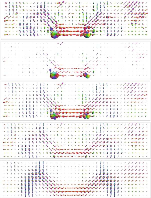

  

  Top: smooth artificial input. Middle: Output of linear diffusion on squared data-set using the analytic kernel approximations of Theorem 11. Bottom: Output erosion applied to the diffused dataset in the middle. Parameter settings for the linear diffusion (t,D ³³,D ⁴⁴)=(0.5,1,0.04). Parameter settings erosion (t,D ¹¹,D ⁴⁴)=(2,0.6,0.3), Δt=0.1

• Morphological scale spaces are preferable over greyscale transformations (such as squaring) for sharpening DW-MRI. They do not amplify large (isotropic) glyphs (Figs. 4 and 23) and they allow control over both angular and spatial sharpening of the fibers via the coefficients (D ¹¹,D ⁴⁴) (Fig. 14).

  Fig. 23

  

  First row: Input DTI-dataset of a human brain. Displayed are the corpus callosum and the corona radiata, measured with a b-value of 1000 s/mm² in 49 gradient directions on voxels of (2mm)³. Second row: squared input data. Third row: result nonlinear diffusion [26] (D ⁴⁴,t,K)=(0.002,3,0.05). Fourth row: result erosion with (D ⁴⁴,t)=(0.002,3). Fifth row: output nonlinear diffusion when using the fourth row as input with (D ⁴⁴,t,K)=(0.002,3,0.1). We used spatial step-size h=0.88, and angular step-size h _a =0.1, cf. Eq. (85). We always used (D ¹¹,Δt)=(1,0.1) for erosion and (D ³³,Δt)=(1,0.01) for nonlinear diffusion. In contrast to the experiments in Figs. 4, 5, 6, 21, and previous work [65, 68] we did not include operator $\mathcal{V}$ Eq. (5) for visualization (we only subtracted the minimum per glyph) and we used Eq. (3) instead of Eq. (4), cf. [26]

• Complex crossing fiber-structures can be extrapolated from DTI by application of scale spaces on ℝ³⋊S ² (Figs. 5, 23).

• Non-aligned glyphs in DW-MRI and spurious non-aligned crossings in HARDI are removed by left-invariant diffusion on ℝ³⋊S ² (Figs. 5, 21, 23 and 6).

• Our extended model for contour completion provides a more reasonable completion of gaps in fibers (Fig. 20).

12 Conclusion

We have developed crossing preserving, rotation- and translation covariant scale spaces on DW-MRI images. The underlying evolutions are convection-diffusion equations and Hamilton-Jacobi-Bellman equations of respectively stochastic and cost processes, on the space of positions and orientations ℝ³⋊S ². These scale spaces are expressed in a moving frame of reference allowing (hypo-elliptic) diffusion along fibers and erosion orthogonal to fibers. They extrapolate complex fiber-structures (crossings) from DTI, while reducing non-aligned crossings in HARDI. They can be implemented by finite difference methods [26], or by convolutions with analytic kernels.

We have addressed the nine objectives arising from previous work which are listed in the introduction. The main results of this article are Theorems 10, 11 and 12.

Appendices

Appendix A: Viscosity Solutions of Morphological Scale Spaces on ℝ³⋊S ²

In this section we provide a proof of Theorem 10.

We will generalize the well-known results on viscosity solution of Hamilton-Jacobi-Bellman equations ℝⁿ to ℝ³⋊S ² embedded in SE(3), where we replace the local frame generated by the spatial generators $\partial_{x^{i}}$ by the moving frame of left-invariant vector fields $\mathcal{A}_{i}$. The difficulty is that we do not have a general Hopf-Lax formula with a scaled Lagrangian as in [39, Theorem 4] at hand, and moreover we do not have a tangible explicit formula for the exact Green’s function.

However, the proof [39, pp. 561–563] of viscosity solution of Hamilton-Jacobi-Bellman equations on ℝⁿ primarily requires the limiting behavior

(95)

of the morphological Green’s function

$$k_{t}(\mathbf{x})= \frac{2\eta-1}{2\eta } t^{-\frac{1}{2\eta-1}}\|\mathbf{x}\|^{\frac{2\eta}{2\eta-1}}. $$

This is where Theorem 11 comes into play. The logarithmic modulus approximations provide lower and upper-bounds for the exact morphological Green’s functions. By Theorem 9 the exact Green’s functions arise by geodesically equidistant propagation of the morphological delta, δ ^C given by Eq. (25). Moreover, the logarithmic modulus approximations arise by freezing the coefficients $p \mapsto\dot{\gamma}^{i}(p)$. These approximations are accurate for small h. In fact, we have the following generalization of Eq. (95) to ℝ³⋊S ²:

Lemma 5

Let c ⁱ∈ℝ, i=1,2,4,5 and $\eta>\frac{1}{2}$ and define $\overline{\mathcal{L}}_{\eta}:\mathbb{R}^{4} \to\mathbb {R}^{+}$ by

then the exact morphological Green’s function on SE(3) given by

(96)

y∈ℝ³,R∈SO(3),h>0 given by Eq. (69) satisfies

Proof

Consider Eq. (63) (and Eq. (46)), then to each C ²-curve with $\langle \mathrm{d}\mathcal{A}^{3}\vert _{\gamma}, \dot {\gamma} \rangle =\langle \mathrm{d}\mathcal{A}^{6}\vert _{\gamma}, \dot {\gamma} \rangle=0$, we have the following C ¹-functions

for i∈{1,2,4,5}. Let ψ:ℝ⁺→ℝ⁺ be the local smooth map that maps spatial arc length s to arclength p in the sub-Riemannian manifold $(\mathrm{SE}(3), \mathrm{d}\mathcal{A}^{3},\mathrm{d}\mathcal{A}^{6})$. This map is a diffeomorphism until the first cusp-time arises (likewise in Fig. 11). Application of first order Taylor-approximation around s=0 yields

and $\eta>\frac{1}{2}$ implies that this is of the order

where ψ ⁻¹(0)=0 and in the interior of a minimizing curve we have finite curvature so ψ ⁻¹(h)=O(h) and the first term vanishes as h↓0 and the result follows from the definition of the morphological kernel, Eq. (63). □

Remark

In the subsequent proofs we need a sober notation and we just write

for all g∈SE(3), (y,n)∈ℝ³⋊S ² and all t≥0, for the corresponding morphological Green’s function on the group SE(3), given in Eq (96).

A second issue is the semi-group property. The PDE for morphological scale spaces is a non-linear evolution and the question whether the semi-group property (57) that holds for linear left-invariant evolutions has a morphological counterpart, i.e. whether Eq. (71) holds. In the ℝⁿ case, this directly follows from the isomorphic properties of the Cramer transform [5, 17], but in ℝ³⋊S ² this is difficult.

Lemma 6

The exact erosion/dilation kernels $k_{t}^{D^{11},D^{44},\eta,\pm }:\mathbb{R}^{3}\rtimes S^{2} \to\mathbb{R}^{+}$ satisfy the semigroup property Eq. (71).

Proof

Let $\tilde{k}_{t}:\mathrm{SE}(3)\to\mathbb{R}^{+}$ be the corresponding kernels on the group according to Eq. (96). Define

for all g∈SE(3) and t≥0, then the semi-group property follows from

(97)

for all τ∈[0,t] and the associativity of morphological convolutions. So it remains to prove Eq. (97). To this end we follow a similar approach as in [56, Theorem 1] (avoiding specific scaling properties of the Lagrangian). By Theorem 9 it follows that the Green’s functions are induced by geodesically equidistant propagation of the morphological delta, δ ^C given by Eq. (25). More precisely, they are given by Eq. (69).

In general one has

(98)

for all g,h,v∈SE(3) and all τ∈[0,t], since the concatenation of two optimal curves yields an admissible curve over which the left hand side is optimized. Here equality is obtained if v ⁻¹ q is on the minimizing curve between e and v ⁻¹ g, i.e. by left-invariance g is on the minimizing curve between e and v ⁻¹ g. Now due to continuity and convexity of $(c^{1},c^{2},c^{4},c^{5}) \mapsto\overline{\mathcal {L}}_{\eta}(c^{1},c^{2},c^{4},c^{5})$ the infimum in (97) is actually a minimum and therefore we can choose v∈SE(3) such that

Then by Eq. (98) one has

for all q∈SE(3) and thereby (by taking the infimum over all q) we obtain

(99)

In order to prove (57) it remains to be shown that

Let w∈SE(3) such that

Now take q as a point along the minimizing curve between g and w. Then we have

from which the result follows. □

To complete the proof of Theorem 10 we must prove the following theorem.

Theorem 13

The viscosity solutions of

(100)

for all t≥0, (y,n)∈ℝ³⋊S ², are respectively given by left-invariant erosion (cf. Eq. (24))

(101)

and left-invariant dilation (cf. Eq. (23))

(102)

with the morphological Green’s functions.

Proof

The proof consists of two parts, first we must show that they are indeed solutions and then we show that they are viscosity solutions. We will only consider the erosion case since the dilation case can be treated analogously.

Part I

This part consists of two subparts. In part Ia we will show that if we set

$$ W(\mathbf{y},\mathbf{n},t):=\bigl(k_{t}^{D^{11}, D^{44}, \eta, +} \ominus_{\mathbb{R}^{3} \rtimes S^2}U\bigr) (\mathbf{y},\mathbf{n}) $$

with morphological kernel given by Eq. (69), then

$$ \frac{\partial W}{\partial t}(\mathbf{y},\mathbf{n},t) \mp\mathcal {H}_{\eta}\bigl(\mathrm{d}\tilde{W}(\mathbf{y},R_{\mathbf{n}},t)\bigr) \leq0. $$

(103)

In part Ib we show the remaining part

$$ \frac{\partial W}{\partial t}(\mathbf{y},\mathbf{n},t) \mp\mathcal {H}_{\eta}\bigl(\mathrm{d}\tilde{W}(\mathbf{y},R_{\mathbf{n}},t)\bigr) \geq0. $$

(104)

Part Ia

Again we resort to evolutions on the full group SE(3) by setting $\tilde{W}(\mathbf{y},R,t)=W(\mathbf{y},R\mathbf{e}_{z},t)$ for all y∈ℝ³, R∈SO(3), t>0. Then for all A=∑ _{i∈{1,2,4,5}} c ⁱ A _i one has by Lemma 6 that

for all g=(y,R) and consequently, one has

$$ \frac{\tilde{W}(ge^{hA},t+h)-\tilde{W}(g,t)}{h} \leq\frac{\tilde {k}_{h}(e^{h A})}{h} $$

and thereby, by Lemma 5 and the construction of the left-invariant vector fields by means of the derivative of the right regular representation $\mathcal{A}_{i}=\mathrm{d}\mathcal{R}(A_{i})$ one gets

$$ \frac{\partial\tilde{W}(g,t)}{\partial t}+ c^{i} \mathcal {A}_{i} \vert _{g} \tilde{W}(g,t) \leq\overline{\mathcal{L}}_{\eta }( \mathbf{c}) $$

(105)

for all c=(c ¹,c ²,c ⁴,c ⁵)∈ℝ⁴. So by subtracting the Lagrangian and taking the maximum over all c we apply the Fenchel transform of the Lagrangian $\mathcal{L}_{\eta}$ which, according to Theorem 8), yields the Hamiltonian $\mathcal{H}_{\eta}$ evaluated at $\mathbf{p}=\mathrm{d}\tilde {W}(\mathbf{y},R_{\mathbf{n}},t)$ and Eq. (103) follows.

Part Ib

Let $g^{*}=(\mathbf{y}^{*},R_{\mathbf {n}^{*}}) \in \mathrm{SE}(3)$ be the minimizer in the erosion operator, i.e.

$$ \tilde{W}(g,t)=\tilde{W}\bigl(g^{*},0\bigr)+ \tilde{k}_{t} \bigl(\bigl(g^{*}\bigr)^{-1} g\bigr). $$

Then we have

where g,g ^∗∈SE(3) are given by

If we now let h↓0 then we obtain

(106)

where we applied Lemma 6 and where we note that the Campbell-Baker-Hausdorff formula

implies that

for almost every g∈ℝ³⋊S ² (where $\tilde{W}(\cdot,t-h)$ is differentiable).

Recall that the left-invariant vector fields are obtained by the derivative of the right-regular representation $\mathcal{A}_{i}=\mathrm{d}\mathcal{R}(A_{i})$, $A_{i}= \mathcal {A}_{i}\vert _{(0,I)}$ and as a result the limit in the left-hand side of (106) equals

Furthermore, we assume without loss of generality that c ³=c ⁶=(c ^∗)³=(c ^∗)⁶=0, i.e.

(107)

Recall that ℝ³⋊S ²=SE(3)/({0}×SO(2)) and $\tilde{W}(g,t)=W(\mathbf{y},R \mathbf {e}_{z},t)$, g=(y,R)∈SE(3) so that

for all α,β∈ℝ and by the Campbell-Baker-Hausdorff formula one can always find α,β∈ℝ such that

justifying our assumption Eq. (107).

Assumption (107) allows us to compute the limit in the final right-hand side of inequality (106) by means of Lemma 5 and we obtain

from which we conclude:

from which the result (104) follows.

Part II

Next we verify that erosion (102) with the Green’s function k _t indeed satisfies (64) at a location (y ₀,n ₀,t ₀)∈(ℝ³⋊S ²)×R ⁺ where W−V attains a local maximum. The dilation case follows analogously.

First of all it follows by left-invariance (and the fact that SE(3) acts transitively on ℝ³⋊S ², cf. Eq. (6)) that without loss of generality we can restrict ourselves to the case (y ₀,n ₀)=(0,e _z ). Secondly, by the semigroup property in Lemma 6, we only need to consider the case t ₀=0, while dropping the constraint t>0.

Since W−V attains a maximum in (0,e _z ,0), there exists a small open set Ω around (0,e _z ,0) in (ℝ³⋊S ²)×ℝ where

(108)

for −ϵ ₁<t<0 for ϵ ₁>0 small enough. Furthermore, we have by Eq. (101) that

(109)

for all (y,n)∈ℝ³⋊S ². Combining the estimates (108) with (109) yields

(110)

locally around (0,e _z ,0), that is within Ω. Or equivalently for the corresponding function on SE(3) given by $\tilde{V}(\mathbf{x},R,t)=V(\mathbf{x},R\mathbf {e}_{z},t)$ we have

(111)

for |t|∈[0,ϵ ₁),d _SE(3)(y,R _n ,(0,I))<ϵ ₂, for some ϵ ₁>0, ϵ ₂>0. Now set

and take the limit h↓0 then we obtain

where we applied Lemma 5. Now the left-invariant vector fields are given by the derivative of the right regular representation $\mathcal{A}_{i}=\mathrm{d}\mathcal{R}(A_{i})$ with $\mathcal {A}_{i}\vert _{(\mathbf{0},I)}=A_{i}$, so by taking the supremum over all A (or (c ¹,c ²,c ⁴,c ⁵)) we obtain

(112)

with $\mathrm{d}\tilde{V}(\cdot,t)=\sum_{i=1}^{5} A_{i}\tilde {V}(\cdot,t)\mathrm{d}A^{i} \in T_{e}^{*}(\mathrm{SE}(3))$. Now by Theorem 8 it follows that

(113)

As a result we conclude that the erosions Eq. (101) with the morphological kernel (69) are the (unique, [24, 39]) viscosity solutions of the Hamilton-Jacobi-Bellman equations (100) on the sub-Riemannian manifold $(\mathbb{R}^{3}\rtimes S^{2},\mathrm{d}\mathcal {A}^{3})$.  □

Appendix B: Propagation of geodesically equidistant surfaces

In this section we provide a proof of Theorem 9.

First of all we note that Eq. (62) in Definition 7 can be written out in more explicit form via the chain-rule for differentiation

(114)

from which we deduce that

(115)

where D _X denotes the derivative w.r.t. a vector field X tangential to a transversal minimizing geodesic γ given by

for 0≤p≤t+ϵ, with ϵ>0. Here γ is a minimizing curve of Eq. (46) for suitable beginning and ending conditions. Then we can rewrite Eq. (62) and Eq. (114) explicitly in components as

Definition 7 allows a re-parameterization of time and by Eq. (49) we can use $\mathcal{L}_{\eta}$ in stead of $\tilde{\mathcal{L}}_{\eta}$. Now the surfaces are geodesically equidistant if and only if for all minimizing (transversal) geodesics one has

where we used the Fenchel transform in Eq. (8), Theorem 8 and Eq. (115) in the second equality. Varying the boundary-conditions of the minimizing geodesics provide the required result.

Appendix C: Pseudo-linear Scale Spaces

So far we have considered anisotropic diffusions aligned with fibers and erosions orthogonal to the fibers. As these two types of left-invariant evolutions can be concatenated, cf. Fig. 4, the natural question arises whether there exist a single evolution process that combines erosion/dilation and diffusion. Moreover, a simple alternative to visually sharpen distributions on positions and orientations is to apply monotonic greyvalue transformations, for instance via the power operator $\tilde{\chi }_{q}$

where q≥1, where we recall its drawback illustrated in Fig. 4. Conjugation of the diffusion operator with a monotonically increasing grey-value transformation χ:ℝ⁺→ℝ⁺

(116)

is related to simultaneous erosion/dilation and diffusion, cf. [40]:

Theorem 14

Let $Q^{\mathbf{D},\mathbf{0}}(\underline{\mathcal{A}})$ be a legal diffusion generator, as in Theorem 4, with $\mathbf {D}=\operatorname{diag}\{D^{11},D^{11},0,D^{33},D^{44},D^{44}\}$. Then the pseudo-linear scale spaces given by

(117)

with C∈ℝ, t≥0, are solved by

where χ _C :ℝ⁺→ℝ⁺ denotes the monotonic greyvalue transformation in the co-domain given by

whose inverse is given by

Proof

This is a straightforward generalization of the derivations in [40] where one replaces the shift-invariant generators $\partial_{x^{i}}$ on ℝⁿ by the left-invariant generators $\{\mathcal {A}_{i}\}_{i=1}^{6}$ on SE(3). The derivations in [40] rely on the chain-law for monotonic transformations in the codomain and the product rule for differentiation and these rules also apply to $\{\mathcal{A}_{i}\}_{i=1}^{6}$. Finally, the solution of the pseudo-linear scale space is legal (Definition 3) iff the diffusion operator $e^{t Q^{\mathbf{D},\mathbf {a}}(\underline{\mathcal{A}})}$ is legal. □

Remark

The drawback of this correspondence, is that our diffusions primarily take place along the fibers, whereas our erosions take place orthogonal to the fibers, recall Fig. 10. The pseudo-linear scale spaces always erode/dilate (depending on $\operatorname{sign}(C)$) and diffuse in the same direction.

Appendix D: Scale Space Definitions

We use the following definitions for scale spaces on the coupled space of positions and orientations.

Definition 12

A scale space representation W:ℝ³⋊S ²×ℝ⁺→ℝ⁺ of initial condition W(⋅,0):=U is the solution of a left-invariant evolution system, with U↦Φ _t (U):=W(⋅,t) left-invariant and Φ _t+s =Φ _t ∘Φ _s for all s,t≥0.

If Φ _t is a linear, mass-preserving, evolution generated by a negative definite, (hypo)elliptic differential operator, W is called a linear scale space representation of U.

If Φ _t is the viscosity solution operator to a Hamilton-Jacobi-Bellmann system, given by morphological convolution with the corresponding morphological Green’s function, W is called a morphological scale space representation of U.

References

Aganj, I., Lenglet, C., Jahanshad, N., Yacoub, E., Harel, N., Thompson, P., Sapiro, G.: A hough transform global probabilistic approach to multiple-subject diffusion MRI tractography. Med. Image Anal. 15(4), 414–425 (2011)
Agrachev, A., Boscain, U., Gautier, J.-P., Rossi, F.: The intrinsic hypoelliptic Laplacian and its heat kernel on unimodular Lie groups. J. Funct. Anal. 256, 2621–2656 (2009)
Astola, L., Florack, L.M.J.: Finsler geometry on higher order tensor fields and applications to high angular resolution diffusion imaging. Int. J. Comput. Vis. 92(3), 325–336 (2011)
Agrachev, A.A., Sachkov, Y.L.: Control Theory from the Geometrical Viewpoint vol. 87. Springer, Berlin (2004)
Akian, M., Quadrat, J., Viot, M.: Bellman processes. Lect. Notes Control Inf. Sci. 199, 302–311 (1994)
Alexander, D.C., Barker, G.J., Arridge, S.R.: Detection and modeling of non-Gaussian apparent diffusion coefficient profiles in human brain data. Magn. Reson. Med. 48, 331–340 (2002)
van Almsick, M.A.: Context models of lines and contours. Ph.D. thesis, Eindhoven University of Technology, Dept. of Biomedical Engineering, Eindhoven, The Netherlands (2005). ISBN:978-90-386-1117-4
Alvarez, L., Guichard F, F., Lions, P.L., Morel, J.-M.: Axioms and fundamental equations of image processing. Arch. Ration. Mech. Anal. 123, 200–257 (1993)
Aubin, T.: In: A Course in Differential. Geometry Graduate Studies in Mathematics, AMS, vol. 27 (2001)
August, J.: The curve indicator random field. Ph.D. thesis, Yale University (2001)
Basser, P.J., Matiello, J., Lebihan, D.: MR diffusion tensor spectroscopy and imaging. Biophys. J. 66, 259–267 (1994)
Bellaïche, B.: The Tangent Space in Sub-Riemannian Geometry. Progress in Mathematics. Birkhauser, New York (1996)
Gromov, M.: Carnot-Caratheodory Spaces Seen from Within. Bellaïche, A., Risler, J.-J. (eds.): In Sub-Riemannian Geometry, Progress in Mathematics. Birkhauser, Basel (1996)
Boscain, U., Charlot, G., Rossi, F.: Existence of planar curves minimizing length and curvature, differential equations and dynamical systems, collected papers. In: Tr. Mat. Inst. Steklova, vol. 270, pp. 49–61. MAIK Nauka/Interperiodica, Moscow (2010)
Boscain, U., Duits, R., Rossi, F., Sachkov, Y.: Optimal control for reconstruction of curves without cusps. In: Astolfi et al. (eds.) IEEE Conf. on Decision and Control, Maui, Hawaii (2012, to appear). Accepted for publication
Bryant, R., Griffiths, P.: Reduction for constrained variational problems and (1/2)∫κ 2 ds. Am. J. Math. 108(3), 525–570 (1986)
Burgeth, B., Weickert, J.: An explanation for the logarithmic connection between linear and morphological systems. In: Proc. 4th Int. Conference Scale Space 2003. Lecture Notes in Computer Science, pp. 325–339. Springer, Berlin (2003)
Burgeth, B., Didas, S., Weickert, J.: Visualization and processing of tensor fields. In: A General Structure Tensor Concept and Coherence-Enhancing Diffusion Filtering for Matrix Fields, pp. 305–324. Springer, Berlin (2009)
Burgeth, B., Breuss, M., Pizarro, L., Weickert, J.: PDE-Driven adaptive morphology for matrix fields. In: Proc. Scale Space and Variational Methods in Computer Vision. Lecture Notes Computer Science, vol. 5567, pp. 247–258. Springer, Berlin (2009)
Burgeth, B., Pizarro, L., Didas, S., Weickert, J.: Coherence-enhancing diffusion for matrix fields. Florack, et al. (eds.): In: Mathematical Methods for Signal and Image Analysis and Representation Springer, Berlin (2012)
Chirikjian, G.S., Kyatkin, A.B.: Engineering Applications of Noncommutitative Harmonic Analysis: with Emphasis on Rotation and Motion Groups. CRC Press, Boca Raton (2001)
Chirikjian, G.S.: Stochastic models, information theory and Lie groups. In: Applied and Numerical Harmonic Analysis. Birkhäuser, Berlin (2009)
Citti, G., Sarti, A.: A cortical based model of perceptional completion in the roto-translation space. J. Math. Imaging Vis. 24(3), 307–326 (2006)
Crandall, M.G., Lions, P.-L.: Viscosity solutions of Hamilton-Jacobi equations. Trans. Am. Math. Soc. 277(1), 1–42 (1983)
Creusen, E.J., Duits, R., Dela Haije, T.C.J.: Numerical schemes for linear and non-linear enhancement of DW-MRI. In: Scale Space and Variational Methods in Computer Vision. Lecture Notes in Computer Science, vol. 6667, pp. 14–25. Springer, Heidelberg (2011)
Creusen, E.J., Duits, R., Florack, L.M.J., Vilanova, A.: Numerical schemes for linear and non-linear enhancement of DW-MRI. Numer. Math. Theor. Method Appl. (2012, to apear)
Dela Haije, T.C.J., Duits, R., Tax, C.M.W.: Sharpening fibers in diffusion weighted MRI via erosion. Submitted book chapter to “Visualization and Processing of Tensors and Higher Order Descriptors for Multi-Valued Data”, Dagstuhl Seminar 11501. URL: http://bmia.bmt.tue.nl/people/RDuits/JMIVDuits2011final.pdf
Descoteaux, M., Angelino, E., Fitzgibbons, S., Deriche, R.: Regularized, fast, and robust analytical Q-ball imaging. Magn. Reson. Med. 58(3), 497–510 (2007)
Descoteaux, M.: High angular resolution diffusion MRI: from local estimation to segmentation and tractography. Ph.D. Thesis, Universite de Nice, Sophia Antipolis, Febuary (2008)
Duits, R., Florack, L.M.J., de Graaf, J., ter Haar Romeny, B.M.: On the axioms of scale space theory. J. Math. Imaging Vis. 20, 267–298 (2004)
Duits, R.: Perceptual organization in image analysis. Ph.D. Thesis, Eindhoven University of Technology, Department of Biomedical Engineering, The Netherlands (2005). A digital version is available on the web URL: http://www.bmi2.bmt.tue.nl/Image-Analysis/People/RDuits/THESISRDUITS.eps
Duits, R., Franken, E.M.: Left invariant parabolic evolution equations on SE(2) and contour enhancement via invertible orientation scores, part I: linear left-invariant diffusion equations on SE(2). Q. Appl. Math. AMS 68(2), 255–292 (2010)
Duits, R., Franken, E.M.: Left invariant parabolic evolution equations on SE(2) and contour enhancement via invertible orientation scores, part II: nonlinear left-invariant diffusion equations on invertible orientation scores. Q. Appl. Math. AMS 68(2), 293–331 (2010)
Duits, R., van Almsick, M.A.: The explicit solutions of linear left-invariant second order stochastic evolution equations on the 2D-Euclidean motion group TU/e. Dept. W&I, CASA-report (2005). http://www.win.tue.nl/analysis/reports/rana05-43.pdf
Duits, R., van Almsick, M.: The explicit solutions of linear left-invariant second order stochastic evolution equations on the 2D-Euclidean motion group. Q. Appl. Math. Am. Math. Soc. 66, 27–67 (2008)
Duits, R., Franken, E.M.: Left-invariant diffusions on the space of positions and orientations and their application to crossing-preserving smoothing of HARDI images. Int. J. Comput. Vis. 92(3), 231–264 (2011). See http://www.springerlink.com/content/511j713042064t35/
Duits, R., Creusen, E., Ghosh, A., Dela Haije, T.: Diffusion, convection and erosion on SE(3)/({0}×SO(2)) and their application to the enhancement of crossing fibers (2011). arXiv:1103.0656v5
Euler, L.: Methodus inveniedi lineas curvas maximi minimive proprietate gaudentes, sive solutio problematis isoperimitrici latissimo sensu accepti. Lausanne, Geneva (1744)
Evans, L.C.: Partial Differential Equations. Graduate Studies in Mathematics, vol. 19. AMS, Providence (1998)
Florack, L.M.J., Maas, R., Niessen, W.J.: Pseudo-linear scale-space theory. Int. J. Comput. Vis. 31(2/3), 247–259 (1999)
Florack, L.M.J.: Codomain scale space and regularization for high angular resolution diffusion imaging. In: Aja Fernández, S., de Luis Garcia, R. (eds.) CVPR Workshop on Tensors in Image Processing and Computer Vision, Anchorage, Alaska, USA, June 24–26, 2008 IEEE Press, New York (2008). Digital proceedings
Franken, E.M., Duits, R.: Crossing preserving coherence-enhancing diffusion on invertible orientation scores. Int. J. Comput. Vis. 85(3), 253–278 (2009)
Franken, E.: Enhancement of crossing elongated structures in images. Ph.D. Thesis, Department of Biomedical Engineering, Eindhoven University of Technology, The Netherlands, Eindhoven (2008)
Ghosh, A., Dela Haije, T.C.J., Duits, R.: Geodesics on ℝ3⋊S 2. In preparation
Gur, Y., Sochen, N.: Regularizing flows over Lie groups. J. Math. Imaging Vis. 33(2), 195–208 (2009)
Gur, Y., Sochen, N.: Denoising tensors via Lie group flows. In: Variational, Geometric, and Level Set Methods in Computer Vision. LNCS, vol. 3752, pp. 195–208 (2005)
Florack, L.M.J.: Image structure. In: Computational Imaging and Vision Series, vol. 10. Kluwer Academic, Dordrecht (1997)
ter Haar Romeny, B.M., Florack, L.M.J., Koenderink, J.J., Viergever, M.A. (eds.): Scale-Space Theory in Computer Vision: Proc. of the First International Conference, Scale-Space’97, Utrecht, The Netherlands. Lecture Notes in Computer Science, vol. 1252. Springer, Berlin (1997)
Hormander, L.: Hypoelliptic second order differential equations. Acta Math. 119, 147–171 (1968)
Iijima, T.: Basic theory on normalization of a pattern (in case of typical one-dimensional pattern). Bull. Electr. Lab. 26, 368–388 (1962)
Kerckhove, M. (ed.): Scale-Space and Morphology in Computer Vision: Proceedings of the Third International Conference, Scale-Space 2001. Lecture Notes in Computer Science, vol. 2106. Springer, Berlin (2001)
Koenderink, J.J.: The structure of images. Biol. Cybern. 50, 363–370 (1984)
Lenglet, C., Prados, E., Pons, J.-P., Deriche, R., Faugeras, O.: Brain connectivity mapping using Riemannian geometry, control theory, and PDEs. SIAM J. Imaging Sci. 2(2), 285–322 (2009)
Lindeberg, T.: Scale-space for discrete signals. IEEE Trans. Pattern Anal. Mach. Intell. 12(3), 234–245 (1990)
Lindeberg, T.: Scale-Space Theory in Computer Vision. The Kluwer International Series in Engineering and Computer Science. Kluwer Academic, Dordrecht (1994)
Manfredi, J.J., Stroffolini, B.: A version of the Hopf-Lax formula in the Heisenberg group. Commun. Partial. Differ. Equ. 27(5), 1139–1159 (2002)
Medioni, G., Lee, M.-S., Tang, C.-K.: A Computational Framework for Segmentation and Grouping. Elsevier, Amsterdam (2000)
Medioni, G., Lee, M.-S., Tang, C.-K.: Tensor Voting: a Perceptual Organization Approach to Computer Vision and Machine Learning. Synthesis Lectures on Image, Video, and Multimedia Processing, vol. 5. Morgan and Claypool, San Mateo (2011)
Mumford, D.: Elastica and computer vision. In: Algebraic Geometry and Its Applications, pp. 491–506. Springer, Berlin (1994)
Osher, S.J., Fedkiw, R.P.: Level Set Methods and Dynamic Implicit Surfaces. Applied Math. Sciences, vol. 153. Springer, Berlin (2003)
Özarslan, E., Mareci, T.H.: Generalized diffusion tensor imaging and analytical relationships between diffusion tensor imaging and high angular resolution imaging. Magn. Reson. Med. 50, 955–965 (2003)
Petitot, J.: Neurogéomètrie de la Vision–Modèles Mathématiques et Physiques des Architectures Fonctionelles. Les Éditions de l’École Polytechnique, Paris (2008)
Pizarro, L., Burgeth, B., Breuss, M., Weickert, J.: A directional Rouy-Tourin scheme for adaptive matrix-valued morphology. In: Wilkinson, M.H.F., Roerdink, J.B.T.M. (eds.) Proc. Ninth International Symposium on Mathematical Morphology (ISMM 2009). Lecture Notes in Computer Science, vol. 5720, pp. 250–260. Springer, Berlin (2009)
Pontryagin, L.S., Boltyansij, V.G., Gamkrelidze, R.V., Mishchenko, E.F.: The Mathematical Theory of Optimal Processes. Pergamon Press, Oxford (1964)
Prckovska, V., Rodrigues, P., Duits, R., Vilanova, A., ter Haar Romeny, B.M.: Extrapolating fiber crossings from DTI data. Can we infer similar fiber crossings as in HARDI? In: Zhang, G.H., et al. (eds.) CDMRI’10 Proc. MICCAI 2010 Workshop on Computational Diffusion MRI, pp. 26–37 (2010)
Reisert, M., Burkhardt, H.: Efficient tensor voting with 3D tensorial harmonics. In: IEEE Computer Society Conference on Computer Vision and Pattern Recognition Workshops, CVPRW’08, pp. 1–7 (2008)
Reisert, M., Skibbe, H.: Left-invariant diffusion on the motion group in terms of the irreducible representations of SO(3) (2012). Preprint on arXiv:1202.5414v1, see http://arxiv.org/pdf/1202.5414v1.pdf
Rodrigues, P., Duits, R., Vilanova, A., ter Haar Romeny, B.M.: Accelerated diffusion operators for enhancing DW-MRI. In: Bartz, et al. (eds.) Eurographics Workshop on Visual Computing for Biology and Medicine, Leipzig, Germany, pp. 49–56 (2010)
Roerdink, J.B.T.M.: Group morphology. Pattern Recognit. 33, 877–895 (2000)
Moiseev, I., Sachkov, Y.L.: Maxwell strata in sub-Riemannian problem on the group of motions of a plane. ESAIM, Contrôle Optim. Calc. Var. 16(2), 380–399 (2009)
Sachkov, Y.L.: Cut locus and optimal synthesis in the sub-Riemannian problem on the group of motions of a plane. ESAIM, Contrôle Optim. Calc. Var. 17(2) (2011)
Sachkov, Y.L.: Maxwell strata in the Euler elastic problem. J. Dyn. Control Syst. 14(2), 169–234 (2008)
Schur, I.: Arithmische Untersuchen über Endliche Gruppen Linearer Substitionen pp. 164–184. Akad. Wiss., Berlin (1906)
Sethian, J.A.: Level Set Methods and Fast Marching Methods: Evolving Interfaces in Computational Geometry, Fluid Mechanics, Computer Vision and Materials Science. Cambridge University Press, Cambridge (1999)
Tabelow, K., Keller, S.S., Mohammadi, S., Kugel, H., Gerdes, J.S., Polzehl, J., Deppe, M.: Structural Adaptive Smoothing Increases Sensitivity of DTI to Detect Microstructure Alterations. Poster at 17th Annual Meeting of the Organization for Human Brain Mapping Quebec, Canada (2011)
Tabelow, K., Polzehl, J., Spokoiny, V., Voss, H.U.: Diffusion tensor imaging: structural adaptive smoothing. NeuroImage 39(4), 1763–1773 (2008)
Tax, C., Duits, R., Vilanova, A., Leemans, A., ter Haar Romeny, B.M., Ossenblok, P.: Improving and evaluating the reliability of white matter fiber pathways for presurgical planning: application to temporal lobe epilepsy. Preprint available on arXiv
ter Elst, A.F.M., Robinson, D.W.: Weighted subcoercive operators on Lie groups. J. Funct. Anal. 157, 88–163 (1998)
Jackway, P.T.: Morphological Scale-Space. Pattern Recognition, vol. III. Conf. C: Image Speech and Signal Analysis, Proc. 11th IAPR Int. Conf. on Pattern Recognition (1992)
Polzehl, J.: Mathematical Methods for Signal and Image Analysis and Representation, pp. 71–89. Springer, Berlin (2011/2012, in press)
Rund, H.: The Hamiltonian-Jacobi Theory in the Calculus of the Variations. Van Nostrand, London (1966)
Serra, J.: Image Analysis and Mathematical Morphology. Academic Press, San Diego (1982)
van den Boomgaard, R.: The morphological equivalent of the gauss convolution. Nieuw Arch. Wiskd. 10(3), 219–236 (1992)
van Almsick, M.A., Duits, R., Franken, E., ter Haar Romeny, B.M.: From stochastic completion fields to tensor voting. In: Proceedings DSSCC-Workshop on Deep Structure Singularities and Computer Vision, June 9–10, pp. 124–134. Springer, Berlin (2005). Maastricht the Netherlands
Weickert, J.A., Ishikawa, S., Imiya, A.: On the history of Gaussian scale-space axiomatics. In: Gaussian Scale-Space Theory. Computational Imaging and Vision Series, vol. 8, pp. 45–59 (1997)
Welk, M.: Families of generalised morphological scale spaces. In: Griffiths, L.D., Lillholm, M. (eds.) Scale Space Methods in Computer Vision. LNCS, pp. 770–784. Springer, Berlin (2003)
Westin, C.-F., Maier, S.E., Mamata, H., Nabavi, A., Jolesz, F.A., Kikinis, R.: Processing and visualization of diffusion tensor MRI. Med. Image Anal. 6(2), 93–108 (2002)
Acknowledgements
Special thanks to Anna Vilanova, Paulo Rodrigues and Vesna Prčkovska, IST/e, Eindhoven university of Technology for providing the medical data sets and experiments on linear contour enhancement via kernels, cf. [65, 68]. Furthermore, the authors gratefully acknowledge Mark Bruurmijn, Biomedical Engineering at TU/e for his help on DW-MRI visualizations. The European Commission is gratefully acknowledged for supporting Arpan Ghosh under the Initial Training Network-FIRST, Agr.No. PITN-GA-2009-238702.
Open Access
This article is distributed under the terms of the Creative Commons Attribution License which permits any use, distribution, and reproduction in any medium, provided the original author(s) and the source are credited.
Author information
Authors and Affiliations
Corresponding author