From Signatures to Monads in UniMath

Abstract

The term UniMath refers both to a formal system for mathematics, as well as a computer-checked library of mathematics formalized in that system. The UniMath system is a core dependent type theory, augmented by the univalence axiom. The system is kept as small as possible in order to ease verification of it—in particular, general inductive types are not part of the system. In this work, we partially remedy the lack of inductive types by constructing some set-level datatypes and their associated induction principles from other type constructors. This involves a formalization of a category-theoretic result on the construction of initial algebras, as well as a mechanism to conveniently use the datatypes obtained. We also connect this construction to a previous formalization of substitution for languages with variable binding. Altogether, we construct a framework that allows us to concisely specify, via a simple notion of binding signature, a language with variable binding. From such a specification we obtain the datatype of terms of that language, equipped with a certified monadic substitution operation and a suitable recursion scheme. Using this we formalize the untyped lambda calculus and the raw syntax of Martin-Löf type theory.

1 Introduction

The UniMath¹ language is meant to be a core dependent type theory, making use of as few type constructors as possible. The goal of this restriction to a minimal “practical” type theory is to make a formal proof of (equi-)consistency of the theory feasible. In practice, the UniMath language is (currently) a subset of the language implemented by the proof assistant Coq. Importantly, the UniMath language does not include a primitive for postulating arbitrary inductive types. Concretely, this means that the use of the CoqInductive vernacular is not part of the subset that constitutes the UniMath language. The purpose of avoiding the Inductive vernacular is to ease the semantic analysis of UniMath, that is, the construction of models of the UniMath language. Another benefit of keeping the language as small as possible is that it will be easier to one day port the library to a potential proof assistant specifically designed for univalent mathematics.

In the present work, we partially remedy the lack of general inductive types in UniMath by constructing datatypes as initial algebras. We provide a suitable induction principle for the types we construct, analogous to the induction principle the Inductive scheme would generate for us. This way we can construct standard datatypes, for instance the type of lists over a fixed type, with reasonable computational behavior as explained in Sect. 6.1.

Intuitively, datatypes are types of tree-shaped data, and inductive datatypes limit them to well-founded trees; here we exemplify two use cases:

• Structured collections of homogeneous data, e. g., lists of elements of a fixed type:

  

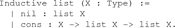
  There are also many kinds of branching data structures for organizing homogeneous data.

• Representations of mathematically interesting objects, e. g., natural numbers and lambda terms (see Example 14 for a categorical presentation) where the type parameter represents the names of the variables that may occur free in them:

  

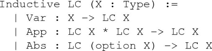
  Here +option X+ is +X+ together with one extra element. This is an example of a “nested datatype” (see Sect. 4.5).

There are two ways to characterize (or specify) inductive datatypes: either externally, via inference rules, or internally, via a universal property. The relationship between the two ways was studied in [7]. There, the authors do not ask whether (some) inductive types are derivable in univalent mathematics. Instead, they start with a basic type theory with the axiom of function extensionality, and present two extensions of that type theory by axioms postulating inductive types, in two different ways: first by axioms mimicking the inference rules, that is, by an internal variant of an external postulate, and second by axioms postulating existence of initial algebras for polynomial functors. The authors then show that those extensions are (logically) equivalent. In the present work, we are interested in an internal characterization of datatypes, as initial objects, and we construct suitable initial algebras.

An inductive datatype has to come with a recursion principle (a calculational form of the universal property) which ought to be mechanically derived together with the datatype itself. Doing this by hand on a case-by-case basis means doing similar tasks many times. For the research program that tries to avoid this “boiler plate” of multiple instances of the same higher-level principles, the name “datatype-generic programming” has been coined by Roland Backhouse and Jeremy Gibbons—nicely indicating in what sense genericity is aimed at.

In this work we focus on a particular class of datatypes that represent languages with variable binding. Those datatypes are families of types that are indexed over the type of free variables allowed to occur in the expressions of the language. Variable binding modifies the indexing type by adding extra free variables in the scope of the binder, as seen in the motivating code example +LC+ of representations of lambda terms above.

Still within the target area of datatype-generic programming (and reasoning), but more specifically, the datatypes we focus on in the present work are canonically equipped with a substitution operation—itself defined via a variant of the recursion principle associated to the datatypes (recursion in Mendler-style [23]). This substitution satisfies the laws of the well-known mathematical structure of a monad—an observation originating in [6, 8, 10]. In this work, we not only construct the datatypes themselves, but also provide a monadic structure—both the operations and the laws—on those datatypes.

The datatypes representing languages with binders are specified via a notion of signature. A signature abstractly describes the shape of the trees by specifying

• the type of nodes and

• the “number” of subtrees of a node.

In the present work, we consider two notions of signatures, and relate them by constructing a function from one type of signatures to the other. One notion is that of a binding signature (cf. Definition 1), a simple notion of signature for which we know how to construct their associated datatypes. The other notion is that of a signature with strength (cf. Definition 4), introduced in [22]. The latter is a more general notion of signature which comes with information on how to perform substitution on the associated language (or, more generally, on any “model” of the signature—even including coinductive interpretations of languages with non-well-founded trees. Coinductive datatypes, however, are not studied in the present work).

Outline of the paper  The present work is built on top of existing work. Here, we list previous work as well as work done for this article, in order to give a coherent picture:

• (i) Section 2 introduces the notions from univalent foundations that we use in the paper. It also describes the UniMath language and its implementation in the Coq proof assistant.

• (ii) In Sect. 3, we construct a signature with strength from a binding signature. This involves constructing an endofunctor on the category of endofunctors on a base category ${\mathcal {C}}$ from a family of lists of natural numbers, as well as a strength (a natural transformation with extra properties) between suitable functors.

• (iii) Instantiating the base category ${\mathcal {C}}$ of the previous section to ${\mathsf {Set}}$, we construct the datatype, as an initial algebra of the endofunctor on endofunctors on the category of sets that is specified by a binding signature, using just the type constructors available in the UniMath language. In particular, we do not use the Coq vernacular Inductive. This work is reported on in Sect. 4.

• (iv) In previous work [4, 22], a model (“substitution system”) of a signature with strength was constructed on a hypothetical initial algebra. This construction was carried out over an arbitrary base category, which, by hypothesis, is sufficiently well-behaved. In particular, right Kan extensions were required to exist. In the present work, we base the needed scheme of generalized iteration in Mendler-style on another theorem in [11] that is based on cocontinuity assumptions instead of the existence of right Kan extensions. We apply this modified construction to the datatype constructed in (iii), where the base category is the category of sets. We hence have to provide the prerequisites for that general construction, in particular, we show that precomposition with a functor preserves colimits of any kind (while only preservation of initial objects and colimits of chains is required for the iteration scheme). This work is reported on in Sect. 5.1.

• (v) In previous work [4, 22], a monad was constructed from any substitution system over an arbitrary base category—thus showing that the substitution constructed in (iv) satisfies widely recognized minimum requirements on substitution. The modified construction of the present work can be applied to our more specific situation without any further conceptual work, see Sect. 5.2.

The construction of (indexed) set-level datatypes described in item (iii) is done by combining two results:

• a classical category-theoretic result saying that an initial algebra of an $\omega$-cocontinuous functor can be constructed from a colimit of a certain chain (i. e., a countably infinite linear diagram) [1];

• the constructibility of colimits in the category of sets (a.k.a. discrete types) in UniMath as a consequence of the constructibility of set quotients.

The construction of set quotients was done by Voevodsky [30]. It is an example of the new possibilities that the univalence axiom and its consequences provide for the formalization of (set-level) mathematics compared to the type theories implemented by Coq or Agda without the univalence axiom.

The reason our construction only works for constructing set-level datatypes is first of all that general types and functions between them do not form a category (as defined in Sect. 2.6). The problem is that the function type $A \rightarrow B$ does not generally form a set for arbitrary types A and B. Second, it is not clear how to construct colimits (in particular, coequalizers) of general types in UniMath (recall that there are no higher inductive types in UniMath ). It is hence not clear if it is possible to directly generalize our construction to arbitrary types.

An alternative approach, not relying on cocontinuity, to constructing W-types in univalent type theory with propositional resizing is presented in [25]. There, the author first constructs non-well-founded trees as in [2], and then carves out the well-founded ones as those trees that satisfy the desired induction principle. This approach does work for arbitrary types, not just for sets. We hope that this work will eventually be formalized in UniMath .

Since we are mainly interested in applying this construction to study languages with binders, the set-level datatypes are sufficient. As explained in point (iv) the theory of cocontinuous functors proved to be useful for other constructions than the construction of datatypes.

On the way to our results, we also deepened the degree of categorical analysis, e. g., we organized the signatures with strength into a category, constructed certain limits and colimits in that category, and identified pointed distributive laws as a means to construct signatures with strength.

The results presented in this article are not surprising—it is our hope, however, that their formalization will be useful and that its underlying ideas extend to richer notions of datatypes and type families. One envisioned use of the library formalized in the present work is outlined in Sect. 6.2.3.

2 About Univalent Foundations and UniMath

The UniMath language is a variation of intensional Martin-Löf type theory [20]. More precisely, there are several versions of the UniMath language: a desired one, used in pen-and-paper reasoning, and one implemented as a ‘subsystem’ of the proof assistant Coq, used for computer-certified proofs in UniMath. The latter provides an approximation of the first, with the long-term goal of closing the gap. Below, we describe the desired theory, and point out the differences to the actual implementation.

The UniMath language is a type theory with

• dependent function types (also called $\varPi$-types) satisfying the $\eta$-rule definitionally;

• dependent pair types (also called $\varSigma$-types) satisfying the $\eta$-rule definitionally;

• intensional identity types;

• coproduct types;

• two universes, one contained in the other, ${\mathcal {U}} _0 : {\mathcal {U}} _1$; universes are closed under the type formers above; more universes can be added as necessary;

• base types: empty, unit, booleans, natural numbers, living in ${\mathcal {U}} _0$;

• strong resizing rules for propositions, see Sect. 2.2;

• the univalence principle for the universes and its consequences, see Sect. 2.3.

Details on the last two items are given in Sects. 2.2 and 2.3 below. Propositional truncation, often assumed as an abstract type former, is implemented in UniMath via impredicativity, cf. Sect. 2.4. Before looking into these points in detail, we fix some vocabulary in Sect. 2.1.

2.1 Fundamental Concepts of Univalent Foundations

In UniMath, types are stratified according to their homotopy level: we say that a type is contractible if it has exactly one element/inhabitant. A type is a proposition if any two of its inhabitants are identical (there need not be any inhabitant, corresponding to an unprovable proposition). A type is a set if all of its identity types are propositions. The hierarchy of homotopy levels continues with groupoids, 2-groupoids and so on, but in the present work these higher levels are not used.

A function $f : A \rightarrow B$ is an equivalence if its fiber over any b : B, $\sum _{a:A} f(a)=b$, is contractible. We denote by $A \simeq B \equiv \sum _{f:A\rightarrow B} {\mathsf {isequiv}}(f)$ the type of equivalences between types A and B. For details we refer to [26, Chapter 2.4].

2.2 Resizing

We distinguish between two kinds of resizing rules:

• Strong resizing denotes resizing rules that change, or specify, the universe a given type lives in. We consider two such rules, formulated by Voevodsky [27]:

  • RR1 Any type X that is a proposition lives in the lowest universe.

  • RR2 For any universe ${\mathcal {U}}$, the ${\mathsf {Prop}} ({\mathcal {U}}) = \sum _{X:{\mathcal {U}}}, {\mathsf {isProp}}(X)$ lives in the lowest universe.

  In [27], Voevodsky sketches a model of some type theory that satisfies these two rules. However, that model does not satisfy the univalence principle. It is currently an open problem whether these rules can consistently be added to a univalent type theory. Furthermore, there is currently no proof assistant implementing these rules.

• Weak resizing denotes rules that state that a given type is equivalent to one in a lower universe. Weak versions of RR1 and RR2 are readily formulated, and are indeed validated in the simplicial set model [18]: there, using classical logic, any proposition is equivalent to either 1 or 0, and the type of propositions of some universe is equivalent to 2. These weak rules would be easy to postulate, as axioms added to the context, in a proof assistant such as Coq. It might, however, be quite cumbersome to work with them in practice. Moreover, weak resizing impedes computation, while good computational behavior even of proofs is a major quality criterion of formalizations in UniMath. This is why Voevodsky preferred strong resizing, as mentioned in his comments to his first implementation of the Foundations Library (the precursor of UniMath)² and to be seen from the focus on strong resizing in [27].

In practice, the UniMath language based on the Coq proof assistant currently lacks any resizing rule (while the design and implementation of a proof assistant based on a universe polymorphic type system with resizing rules was one of the four main goals of the special year on univalent foundations at the Institute for Advanced Study in Princeton³). Instead, it is assumed that all the types are elements of a universe ${\mathcal {U}}$—for sake of simplicity, and while waiting for a satisfying universe mechanism (that supports resizing rules besides universe polymorphism), we even assume the inconsistent typing rule ${\mathcal {U}}:{\mathcal {U}}$. This means that the Coq system does not provide us with a validation of our usage of universes, and we have to do these checks ourselves instead. We claim that we do not exploit the inconsistent typing rule, i.e., that our formalization translates to the theory with strong resizing rules straightforwardly. Throughout the article we point out whenever a construction makes use of the strong resizing rules and we write ${\mathcal {U}}$ for the universes (so the universe level is implicit).

2.3 Univalence

An important part of UniMath is the univalence principle, which characterizes the identity type on the universe ${\mathcal {U}}$. It asserts that the type of identities between types is equivalent to the type of equivalences between those types, and, more precisely, it asserts that the map from identities between types to equivalences between types that is specified by sending the reflexivity to the identity equivalence is an equivalence itself. In particular this means that this map is invertible. In the UniMath library, univalence is added to the context as a Coq axiom.

In the present work, we crucially use some consequences of the univalence axiom that are not provable in pure Martin-Löf type theory. Details are described in Sect. 6.1.

2.4 Propositional Truncation

We call propositional truncation a type transformation that associates to any type A the proposition $\mathopen {}\left\| A\right\| _{}\mathclose {}$. Intuitively, $\mathopen {}\left\| A\right\| _{}\mathclose {}$ is empty when A is, and contractible otherwise—though this is not provable in the theory, as that would require a use of the law of excluded middle. Note that propositional truncation, often postulated as a Higher Inductive Type (HIT) [26, Chapter 6], is implemented in UniMath via a universal quantification, in the style of a generalized double negation:

$$\begin{aligned} \mathopen {}\left\| A\right\| _{}\mathclose {} := \prod \limits _{P : {\mathsf {Prop}} ({\mathcal {U}})} (A \rightarrow P) \rightarrow P , \end{aligned}$$

where we write ${\mathsf {Prop}} ({\mathcal {U}})$ to indicate that we are quantifying over all types of ${\mathcal {U}}$ that are propositions. It is a theorem by Voevodsky that $\mathopen {}\left\| A\right\| _{}\mathclose {}$, thus defined, is again a proposition—however, a proposition living in a universe higher than ${\mathcal {U}}$ unless we use propositional resizing; for a discussion of this issue we refer to [30, Section 4].

The propositional truncation is used to define existential quantification: we write $\exists a : A, B(a)$ for $\mathopen {}\left\| \varSigma _{a:A}B(a)\right\| _{}\mathclose {}$. This allows us to distinguish between structures and properties given by $\varSigma$ and $\exists$. This is also reflected in our use of the vocabulary ‘Problem & Construction’ vs. ‘Theorem & Proof’. Indeed, whenever we describe the construction of a structure, that is, when we construct a term of a type that is not a proposition in the above sense, we use the terminology ‘Problem & Construction’. The pair ‘Theorem & Proof’ is reserved for the construction of inhabitants of a proposition.

2.5 On General Inductive Datatypes

As explained above the general scheme to define strictly positive inductive types and families in Coq, using the Inductive vernacular, is not part of UniMath. Indeed, while the types above are, for technical reasons, implemented in UniMath using the Inductive vernacular, its use is not permitted outside a “preamble” that introduces those types. In this way we simulate a theory in which the above types are primitive rather than an instance of a general type definition mechanism. It is the purpose of the present work to construct some of the inductive types that could otherwise be defined using the Inductive scheme.⁴ Consequently, the experimental HITs are not part of the UniMath language either.

2.6 Category Theory in UniMath

The UniMath library contains a significant amount of category theory, for details see [3]. A category${\mathcal {C}}$ in UniMath is given by:

• a type ${\mathcal {C}} _0$ of objects;

• for any two objects $A,B : {\mathcal {C}} _0$, a set${\mathcal {C}} (A,B)$ of morphisms;

• for any three objects $A,B,C : {\mathcal {C}} _0$, a composition operation

  $$\begin{aligned} {{\_}\mathbin {\circ }{\_}} : {\mathcal {C}} (B,C)\rightarrow {\mathcal {C}} (A,B)\rightarrow {\mathcal {C}} (A,C) \end{aligned}$$

• for any object $A : {\mathcal {C}} _0$, an identity arrow $1_A : {\mathcal {C}} (A,A)$,

subject to the usual axioms of category theory. Functors, natural transformations, etc. are defined in the usual way.

The category ${\mathsf {Set}}$ has as objects sets and as morphisms from X to Y the set of (type-theoretic) functions from X to Y. Given categories ${\mathcal {C}}$ and $\mathcal {D}$, we denote by $[{\mathcal {C}},\mathcal {D}]$ the category of functors from ${\mathcal {C}}$ to $\mathcal {D}$, with natural transformations as morphisms.

The article [3] calls “precategory” the notion here introduced as category, and reserves the word “category” for precategories with an additional property, called “univalence (for categories)”. This property is not relevant for the work reported here. We will occasionally remark on what would be guaranteed in addition for a univalent base category. The category ${\mathsf {Set}}$ is univalent, and univalence is inherited from the target category $\mathcal {D}$ of a functor category $[{\mathcal {C}},\mathcal {D}]$.

We assume the reader to be familiar with the concepts of category theory. Here, we only point to the specific but rather standard notations and conventions we will use throughout.

Instead of writing that F is an object of the functor category $[{\mathcal {C}},\mathcal {D}]$, we often abbreviate this to $F:[{\mathcal {C}},\mathcal {D}]$, but also to $F:{\mathcal {C}} \rightarrow \mathcal {D}$. Given $d : \mathcal {D}$, we call ${\underline{d}} : {\mathcal {C}} \rightarrow \mathcal {D}$ the functor that is constantly d and $1_d$ on objects and morphisms, respectively. This notation hides the category ${\mathcal {C}}$, which will usually be deducible from the context. We write $\mathsf {Id}$ for the identity endofunctor on ${\mathcal {C}}$. We also let (co)product denote general indexed (co)products and explicitly write if they are binary.

The category $\mathrm {Ptd}({\mathcal {C}})$ has, as objects, pointed endofunctors on ${\mathcal {C}}$, that is, pairs of an endofunctor $F : {\mathcal {C}} \rightarrow {\mathcal {C}}$ and a natural transformation $\eta : \mathsf {Id} \rightarrow F$. We write $\mathsf {id}$ for the identity functor with its trivial point and let U be the forgetful functor from $\mathrm {Ptd}({\mathcal {C}})$ to $[{\mathcal {C}},{\mathcal {C}} ]$ (that forgets the point).

Categories, functors and natural transformations constitute the prime example of a 2-category. We write $\mathbin {\circ }$ for vertical composition of natural transformations and $\mathbin {\cdot }$ for their horizontal composition. If one of the arguments to horizontal composition is the identity on some functor, we just write the functor as the respective argument. The corner case where both arguments are the identity on some functors X and Y is just functor composition that is hence written $X\mathbin {\cdot }Y$ (on objects and morphisms, this is X applied after Y, hence $(X\mathbin {\cdot }Y)(A)=X(YA)$ and likewise for morphisms). Horizontal composition of $\mu :F\rightarrow G$ and $\nu :F'\rightarrow G'$ has $\mu \mathbin {\cdot }\nu :F\mathbin {\cdot }F'\rightarrow G\mathbin {\cdot }G'$ provided $F,G:\mathcal {D}\rightarrow \mathcal {E}$ and $F',G':{\mathcal {C}} \rightarrow \mathcal {D}$. The order of vertical composition $\mathbin {\circ }$ is the same as of functor composition: if $F,G,H:{\mathcal {C}} \rightarrow \mathcal {D}$ and $\mu :G\rightarrow H$ and $\nu :F\rightarrow G$, then $\mu \mathbin {\circ }\nu :F\rightarrow H$ is defined by object-wise composition in $\mathcal {D}$.

Given a functor $F : [{\mathcal {A}},{\mathcal {B}} ]$ and a category ${\mathcal {C}}$ we define the functor $\_ \mathbin {\cdot }F$ on functor categories:

$$\begin{aligned} \_ \mathbin {\cdot }F : [{\mathcal {B}},{\mathcal {C}} ] \rightarrow [{\mathcal {A}},{\mathcal {C}} ] \end{aligned}$$

This functor takes a functor $X : [{\mathcal {B}},{\mathcal {C}} ]$ and precomposes it with F, that is, $X \mapsto X\mathbin {\cdot }F$, and likewise with the morphisms, i. e., the natural transformations. Once again the category ${\mathcal {C}}$ is hidden, but it can often be deduced from the context.

We follow [4] in making explicit the monoidal structure on functor category $[{\mathcal {C}},{\mathcal {C}} ]$ that carries over to $\mathrm {Ptd}({\mathcal {C}})$: let $\alpha _{X,Y,Z} : X \mathbin {\cdot }(Y \mathbin {\cdot }Z) \simeq (X \mathbin {\cdot }Y) \mathbin {\cdot }Z$, $\rho _X : 1_{{\mathcal {C}}} \mathbin {\cdot }X \simeq X$ and $\lambda _X : X \mathbin {\cdot }1_{{\mathcal {C}}} \simeq X$ denote the monoidal isomorphisms. Notice that all those morphisms are pointwise the identity, but making them explicit is needed for typechecking in the implementation [4].

3 Two Notions of Signatures

As outlined in the introduction, a signature abstractly specifies a datatype by describing the shape of elements of that type. We give two notions of signatures suitable for the description of languages with variable binding, such as the untyped lambda calculus. We first describe a rather syntactic notion of signature: binding signatures. We then proceed with a description of a semantic notion of signature: signatures with strength. We give constructions to obtain signatures with strength and finally associate a signature with strength to each binding signature.

3.1 Binding Signatures

A binding signature is given by simple syntactic data that allows one to concisely specify a language with variable binding. Binding signatures are less expressive than the signatures with strength that will be presented in the next section. On the other hand, they are easier to specify.

Definition 1

(Arity, binding signature) An arity is a (finite) list of natural numbers. A binding signature is a family of arities, more precisely, as set I and a function $\mathsf {ar}: I \rightarrow \mathsf {List}({\mathbb {N}})$.

Intuitively, the type I of a binding signature indexes the language constructors, and the function $\mathsf {ar}$ associates an arity to each constructor. Note that we do not need decidable equality on the indexing type.

In UniMath we define this as a nested $\varSigma$-type (with for the universe ${\mathcal {U}}$):

We also define functions for accessing the components of a and a constructor function for constructing one:

This way we can mimic the behavior of Coq ’s Record types which are not part of UniMath as they are defined using Inductive.

We can take the coproduct of two binding signatures by taking the coproduct of the underlying indexing sets, and, for the function specifying the arities, the induced function on the coproduct type.

Example 2

(Binding signature of untyped lambda calculus) The binding signature of the untyped lambda calculus is given by $I:= \{ \mathsf {abs}_{}, \mathsf {app}_{} \}$ and the arity function is

$$\begin{aligned} \mathsf {abs}_{} \mapsto [1] , \mathsf {app}_{} \mapsto [0,0] . \end{aligned}$$

This is to be read as follows: there are—besides variables that are treated generically in Sect. 5.1—two constructors. The first constructor $\mathsf {abs}_{}$, corresponding to lambda abstraction, has just one argument (as $\mathsf {ar}(\mathsf {abs}_{})$ is a one-element list), and this argument can make use of 1 extra variable being bound by the constructor. The second constructor $\mathsf {app}_{}$, corresponding to application, has two arguments, and there is no binding involved.

Example 3

(Binding signature of presyntax of Martin-Löf type theory) The binding signature of Martin-Löf type theory is given in Sect. 5.2, as part of an extended example that uses an infinite index set. Using the coproduct of binding signatures, it can easily be decomposed, in particular, using the binding signature of the untyped lambda calculus as one ingredient.

3.2 Signatures with Strength

The next, more semantic, notion of signature was defined in [22, Definition 5]; there, it was merely called “signature”. In order to explicitly distinguish them from binding signatures, we call them “signatures with strength” here. As a new contribution, we organize the signatures with strength as a category.

Definition 4

(Signatures with strength) Given a category ${\mathcal {C}}$, a signature with strength is a pair $(H,\theta )$ of an endofunctor H on $[{\mathcal {C}},{\mathcal {C}} ]$, called the signature functor, and a natural transformation $\theta _{}: (H {-}) \mathbin {\cdot }U {\sim } \rightarrow H ({-} \mathbin {\cdot }U {\sim })$ between bifunctors $[{\mathcal {C}},{\mathcal {C}} ] \times \mathrm {Ptd}({\mathcal {C}}) \rightarrow [{\mathcal {C}},{\mathcal {C}} ]$ such that $\theta _{}$ is ‘linear’ in the second component.

In more detail, the bifunctors applied to a pair of objects (X, (Z, e)) with $X:[{\mathcal {C}},{\mathcal {C}} ]$ and $(Z,e):\mathrm {Ptd}({\mathcal {C}})$ (X for the argument symbolized by − and (Z, e) for the argument symbolized by $\sim$) yield $HX\mathbin {\cdot }Z$ and $H(X\mathbin {\cdot }Z)$, thus $\theta _{X,(Z,e)}:HX\mathbin {\cdot }Z\rightarrow H(X\mathbin {\cdot }Z)$. By ‘linearity’ of $\theta _{}$ in the second argument we mean the equations

$$\begin{aligned} \theta _{X, \mathsf {id}} = H(\lambda ^{-1}_X) \mathbin {\circ }\lambda _{HX} \end{aligned}$$

(note that $\lambda _{HX}:HX\mathbin {\cdot }1\rightarrow HX$ and $H(\lambda ^{-1}_X):HX\rightarrow H(X\mathbin {\cdot }1)$, using the monoidal isomorphism $\lambda$ introduced in Sect. 2.6) and

$$\begin{aligned} \theta _{X, (Z' \mathbin {\cdot }Z, e' \mathbin {\cdot }e)} = H(\alpha ^{-1}_{X,Z',Z}) \mathbin {\circ }\theta _{X \mathbin {\cdot }Z', (Z, e)} \mathbin {\circ }(\theta _{X, (Z', e')} \mathbin {\cdot }Z) \mathbin {\circ }\alpha _{HX, Z', Z} , \end{aligned}$$

as illustrated by the diagram

Definition 5

(Morphism of signatures with strength) Given two signatures with strength $(H,\theta )$ and $(H',\theta ')$, a morphism of signatures with strength from $(H,\theta )$ to $(H',\theta ')$ is a natural transformation $h : H \rightarrow H'$ such that the following diagram commutes for any $X : [{\mathcal {C}},{\mathcal {C}} ]$ and $(Z,e) : \mathrm {Ptd}({\mathcal {C}})$.

Composition and identity morphisms of signatures with strength are given by composition and identity of natural transformations. This defines the category of signatures with strength.

Examples of signatures with strength are given in [22]. Another way of producing examples is the map defined in Construction 13, which associates a signature with strength to any binding signature.

The signatures with strength do not distinguish between arities and signatures. As developed in [4], there is a way to build a new signature by taking the coproduct of two signatures. Intuitively, and just as for binding signatures, this corresponds to constructing a new language by taking the disjoint union of the language constructors of two given languages. What is new here compared to [4] is the explicitly categorical treatment (i. e., taking into account morphisms of signatures with strength). The construction generalizes easily to the coproduct of an arbitrary family of such signatures:

Definition 6

(Coproduct of signatures with strength) If ${\mathcal {C}}$ has coproducts, then the coproduct of a family of signatures with strength is defined as follows:

• the signature functor is given by the coproduct in the endofunctor category on $[{\mathcal {C}},{\mathcal {C}} ]$ induced by that on ${\mathcal {C}}$;

• the strength is induced by coproduct of arrows.

The strength laws are simple consequences of the strength laws of each member of the family of signatures, and the universal property is readily established.

Definition 7

(Binary product of signatures with strength) If ${\mathcal {C}}$ has binary products, then the binary product of two signatures with strength has, as signature functor, the binary product of the functors of the given signatures. The strength is then induced analogously to coproducts.

By way of iteration, binary products will be used to model multiple arguments of a datatype constructor.

Definitions 6 and 7 entail that the forgetful functor from signatures with strength to endofunctors on $[{\mathcal {C}},{\mathcal {C}} ]$ lifts and preserves coproducts and binary products.

3.3 Signatures with Strength from Binding Signatures

Constructing suitable signatures with strength for a language seems like a daunting task. Fortunately, it is often sufficient to specify the binding signature. The generic solution to the following problem then yields the corresponding signature with strength.

Problem 8

Let ${\mathcal {C}}$ be a category with coproducts, binary products and a terminal object. Given a binding signature, the problem consists in the construction of a signature with strength on ${\mathcal {C}}$. This task is naturally divided into

• (i) the construction of the signature functor H as endofunctor on $[{\mathcal {C}},{\mathcal {C}} ]$ and then

• (ii) the construction of a strength for H.

The problem will be solved where the condition on coproducts for ${\mathcal {C}}$ is reduced to binary coproducts and I-indexed coproducts, for I the respective index set of the binding signature.

Construction 9

(Part (i) of Problem 8) Let $(I,\mathsf {ar})$ be a binding signature. Let i : I. To the list $\mathsf {ar}(i) = [n_1,\ldots ,n_k]$ we associate the functor defined on objects by

$$\begin{aligned} A \mapsto \prod _{1\leqslant j \leqslant k} (X \mathbin {\cdot }\mathsf {option}^{n_j})(A) \end{aligned}$$

Here, the functor $\mathsf {option}: {\mathcal {C}} \rightarrow {\mathcal {C}}$ is defined on objects by $\mathsf {option}(A) := 1 + A$. The product is implemented as an iterated binary product. Put differently, we define a functor

$$\begin{aligned}{}[{\mathcal {C}},{\mathcal {C}} ]&\rightarrow [{\mathcal {C}},{\mathcal {C}} ] \\ X&\mapsto \prod _{1 \leqslant j \leqslant k} X \mathbin {\cdot }\mathsf {option}^{n_j} \end{aligned}$$

The functor associated to the signature $(I,\mathsf {ar})$ is then obtained as the coproduct of the functors associated to each arity,

$$\begin{aligned} H : [{\mathcal {C}},{\mathcal {C}} ]&\rightarrow [{\mathcal {C}},{\mathcal {C}} ] \\ X&\mapsto \coprod _{i : I} \prod _{1 \leqslant j \leqslant \mathsf {length}(\mathsf {ar}(i))} X \mathbin {\cdot }\mathsf {option}^{\mathsf {ar}(i)_j} \end{aligned}$$

For the construction of this functor over the category of sets (i. e., when ${\mathcal {C}} ={\mathsf {Set}}$), it is essential for I to be a set.

As we have just seen, the signature functors H that arise from binding signatures are of a special shape, where the argument X only enters in the form of $X\mathbin {\cdot }\mathsf {option}^n$. This can be exploited in the construction of the strength $\theta$ for H. The right level of generality of this pattern is signature functors H that are given by precomposition with a fixed endofunctor G on ${\mathcal {C}}$, i. e., with $HX=X\mathbin {\cdot }G$. Pointed distributive laws for G to be introduced next will lift to strengths for H, hence providing signatures with strength from a simpler input.

Definition 10

(Pointed distributive law) Let ${\mathcal {C}}$ be a category and $G:[{\mathcal {C}},{\mathcal {C}} ]$. A pointed distributive law for G is a natural transformation $\delta : G\mathbin {\cdot }U{\sim }\rightarrow U{\sim }\mathbin {\cdot }G$ of functors $\mathrm {Ptd}({\mathcal {C}})\rightarrow [{\mathcal {C}},{\mathcal {C}} ]$ such that

$$\begin{aligned} \delta _\mathsf {id} =1_G \end{aligned}$$

and

$$\begin{aligned} \delta _{(Z' \mathbin {\cdot }Z, e' \mathbin {\cdot }e)}= \alpha _{Z', Z,G}\mathbin {\circ }Z'\mathbin {\cdot }\delta _{(Z,e)}\mathbin {\circ }\alpha ^{-1}_{Z',G,Z}\mathbin {\circ }\delta _{(Z',e')}\mathbin {\cdot }Z\mathbin {\circ }\alpha _{G,Z', Z}, \end{aligned}$$

where the second equation is commutation of the following diagram:

Note that, in analogy with the definition of signature with strength, we symbolize the sole argument of the functors as $\sim$. Note that setting $\delta _\mathsf {id}$ to $\rho ^{-1}_G\mathbin {\circ }\lambda _G$ instead of the identity would be to emphasize the monoidal structure on $[{\mathcal {C}},{\mathcal {C}} ]$, but our implementation did not run into problems with our simplified definition (that, anyway, is pointwise identical).

The prime example is with $G=\mathsf {option}$, where

$$\begin{aligned} \delta _{(Z,e)}(A)=[e_{\mathsf {option}(A)}\mathbin {\circ }{\mathsf {inl}} _{1,A} \; , \; Z({\mathsf {inr}} _{1,A})]:\mathsf {option}(ZA)\rightarrow Z(\mathsf {option}(A)), \end{aligned}$$

with the injections ${\mathsf {inl}} _{1,A}$ and ${\mathsf {inr}} _{1,A}$ into $\mathsf {option}(A)$.

The following lemma is obtained by easy calculations.

Lemma 11

Let ${\mathcal {C}}$ be a category, $G:[{\mathcal {C}},{\mathcal {C}} ]$ and $\delta$ a pointed distributive law for G. Let H be precomposition with G, then

$$\begin{aligned} \theta _{X, (Z, e)}:=\alpha _{X, Z,G}\mathbin {\circ }X\mathbin {\cdot }\delta _{(Z,e)}\mathbin {\circ }\alpha ^{-1}_{X,G,Z}, \end{aligned}$$

as illustrated by the diagram

yields a natural transformation, and $(H,\theta )$ is a signature with strength.

Also the next lemma is obtained by easy calculations.

Lemma 12

Let ${\mathcal {C}}$ be a category, $G, G':[{\mathcal {C}},{\mathcal {C}} ]$ with pointed distributive laws $\delta$ and $\delta '$, respectively. Then, the following is a pointed distributive law for $G\mathbin {\cdot }G'$:

$$\begin{aligned} \delta ^\cdot _{(Z,e)}:=\alpha ^{-1}_{Z,G,G'}\mathbin {\circ }\delta _{(Z,e)}\mathbin {\cdot }G'\mathbin {\circ }\alpha _{G,Z,G'}\mathbin {\circ }G\mathbin {\cdot }\delta '_{(Z,e)}\mathbin {\circ }\alpha ^{-1}_{G,G',Z}, \end{aligned}$$

visualized as follows:

Construction 13

(Part (ii) of Problem 8) Let $(I,\mathsf {ar})$ be a binding signature. It suffices to define the signature with strength associated to any $\mathsf {ar}(i)$ for i : I. The signature with strength associated to $(I,\mathsf {ar})$ is then obtained by taking the coproduct of all the signatures with strength associated to $\mathsf {ar}(i)$ as in Definition 6.

Let i : I. Thanks to Definition 7 for binary products, used repeatedly in order to account for multiple arguments (i. e., multiple elements in the list $\mathsf {ar}(i)$), it suffices to define the strength associated to the endofunctor on $[{\mathcal {C}},{\mathcal {C}} ]$, expressed by the term $X\mathbin {\cdot }\mathsf {option}^{n_k}$ in the above construction. However, this is an instance of Lemma 11, with $G=\mathsf {option}^{n_k}$, and the latter is an iterated composition of $\mathsf {option}$ for which the pointed distributive law has been given above. So, Lemma 12 provides a pointed distributive law for $\mathsf {option}^{n_k}$.

Example 14

(The signature with strength for the untyped lambda calculus) Consider the binding signature of Example 2. The signature functor obtained from that binding signature via the map defined in Construction 9 is given by

$$\begin{aligned} X \mapsto X \mathbin {\cdot }\mathsf {option}+ X\times X \end{aligned}$$

We also obtain a strength law for this functor by Construction 13. For more details about this see [22].

The next section is dedicated to the construction of initial algebras for the signature functor associated to a binding signature by Construction 9, culminating in Theorem 43 and Construction 46. In Sect. 5 we then equip those initial algebras with a monad structure.

4 Construction of Datatypes as Initial Algebras

Given a category $\mathcal {D}$, we define the datatype specified by a functor $F : \mathcal {D}\rightarrow \mathcal {D}$ to be any initial algebra of F. Note that by this definition, such datatypes are only defined up to unique isomorphism. A given endofunctor F on $\mathcal {D}$ might or might not admit initial algebras. In this section, we construct initial algebras for signature functors as in Sect. 3, with $\mathcal {D}$ instantiated to the category of endofunctors on the category of sets, hence with category ${\mathcal {C}}$ of the previous section fixed to ${\mathsf {Set}}$. However, the results of this section are stated and proved for arbitrary categories ${\mathcal {C}}$ equipped with suitable structure, and only instantiated to ${\mathsf {Set}}$ in the end.

Our main tool for the construction of initial algebras is Construction 26. That construction yields an initial F-algebra for an $\omega$-cocontinuous endofunctor F from a certain colimit. It hence reduces our task of constructing datatypes (i. e., initial algebras) to the construction of certain colimits (see Sect. 4.3) and to showing that various functors preserve these colimits (see Sects. 4.4 and 4.5).

4.1 Colimits

In our formalization, colimits are parametrized by diagrams over graphs, as suggested by [19, p. 71].

Definition 15

(Graph) A graph is a pair consisting of

• a type $\mathsf {vertex}: {\mathcal {U}}$ representing the vertices and

• a family $\mathsf {edge}: \mathsf {vertex}\rightarrow \mathsf {vertex}\rightarrow {\mathcal {U}}$ representing the edges as a dependent family of types.

A diagram, accordingly, is a map from a graph into the graph underlying a category.

Definition 16

(Diagram) Given a graph G made of $\mathsf {vertex}_G$ and $\mathsf {edge}_G$ and a category ${\mathcal {C}}$, a diagram of shape G in ${\mathcal {C}}$ is a pair consisting of

• a map $\mathsf {dob}: \mathsf {vertex}_G\rightarrow {\mathcal {C}} _0$ and

• a family of maps $\mathsf {dmor}: \prod _{u,v:\mathsf {vertex}_G}\mathsf {edge}_G(u,v) \rightarrow {\mathcal {C}} (\mathsf {dob}(u),\mathsf {dob}(v))$.

Henceforth, we will abbreviate $u:\mathsf {vertex}_G$ by u : G. These definitions are also conveniently represented in UniMath using $\varSigma$-types with suitable accessor and constructor functions:

Definition 17

(Cocone) Given a diagram d of shape G in ${\mathcal {C}}$ made of $\mathsf {dob}_d$ and $\mathsf {dmor}_d$, and an object $C : {\mathcal {C}} _0$, a cocone under d with tip C is given by

• a family of morphisms $a:\prod _{v:G} {\mathcal {C}} (\mathsf {dob}_d(v),C)$ and

• a family of equalities $\prod _{u:G,v:G,e:\mathsf {edge}_G(u,v)} {{a(v)}\mathbin {\circ }{\mathsf {dmor}_d(e)}} = a(u)$.

Let $\mathsf {Cocone}(d,C)$ be the type of cocones under d with tip C.

The equalities in the definition can be depicted as:

We often omit the equalities, denoting a cocone just by its family of morphisms.

Definition 18

(Colimiting cocone) A cocone a under d (of shape G) with tip C is called colimiting if for any cocone $a'$ under d with tip $C'$ there is exactly one morphism $f : {\mathcal {C}} (C,C')$ such that ${{f}\mathbin {\circ }{a(v)}} = a'(v)$ for any v : G. Let $\mathsf {iscolimiting}(d,C,a)$ denote this property.

This definition can be illustrated by the following diagram:

In UniMath we represent this by:

Here is a predicate saying that the type is contractible, in other words that it has only one inhabitant which exactly captures the unique existence of f.

Remark 19

(Uniqueness of colimits) If ${\mathcal {C}}$ is a univalent category [3], and d is a diagram of shape G in ${\mathcal {C}}$, then the type of colimits of d,

$$\begin{aligned} \sum _{C:{\mathcal {C}}}\sum _{a : \mathsf {Cocone}(d,C)}\mathsf {iscolimiting}(d,C,a) , \end{aligned}$$

is a proposition.

Given a functor $F : {\mathcal {C}} \rightarrow \mathcal {D}$, a diagram d in ${\mathcal {C}}$ and a cocone a of d with tip $C : {\mathcal {C}} _0$, then Fa is a cocone under Fd with tip FC in $\mathcal {D}$, where Fa and Fd are defined in the obvious way.

Definition 20

(Preservation of colimits) Fix a graph G. We say that Fpreserves colimits of shape G if, for any diagram d of shape G in ${\mathcal {C}}$, and any cocone a under d with tip C, the cocone Fa is colimiting for Fd whenever a is colimiting for d.

A functor is called cocontinuous if it preserves all colimits. In UniMath:

A functor is called $\omega$-cocontinuous if it preserves colimits of diagrams of the shape

that is, diagrams on the graph where objects are natural numbers and where there is a unique arrow from m to n if and only if $1 + m = n$. We refer to diagrams of this shape as chains.

Actually, in the formalization, the type of arrows from m to n is defined to be the type of proofs that $1 + m = n$, exploiting the fact that the type of natural numbers is a set:

Lemma 21

(Invariance of cocontinuity under isomorphism) Let $F,G : {\mathcal {C}} \rightarrow \mathcal {D}$ be functors, and let $\alpha : F \cong G$ be a natural isomorphism, then G preserves colimits (of a certain shape) if F does.

Note that, as preservation of colimits is a proposition, it suffices for the natural isomorphism $\alpha$ to merely exist for the lemma to hold.

Next, we construct colimits in the functor category from colimits in the target category:

Problem 22

(Colimits in functor categories) Let ${\mathcal {C}}$ be a category, and let $\mathcal {D}$ be a category with all (specified) colimits of a given shape. The problem consists in the construction of colimits of the same shape in the functor category $[{\mathcal {C}},\mathcal {D}]$.

Construction 23

(Solution to Problem 22) The construction of colimits in a functor category is pointwise: the colimit C of a diagram is given, at point $c : {\mathcal {C}} _0$, as the colimit in $\mathcal {D}$ of the diagram obtained by evaluating the diagram in $c : {\mathcal {C}} _0$.

Limits have been formalized in the same way as colimits, that is, parametrized by graphs and diagrams. We have implemented a similar construction for lifting limits to functor categories. We omit the details of the dualization.

In the formalization some (co)limits (e. g., pullbacks and pushouts) are also implemented directly, in addition to them being formalized as a colimit over a specific graph. For instance, binary coproducts are formalized as a type parametrized by two objects in a category, instead of by a diagram on the graph $\mathbf {2}$ with two objects and no non-trivial morphisms. We provide suitable maps going back and forth between the different implementations of (co)limits.

The advantage of formalizing the ‘special’ (co)limits as instances of general ones is that results such as the lifting of (co)limits to functor categories restricts immediately to these (co)limits of special shapes.

On the other hand, the direct formulation is more convenient to work with in practice. In particular, we experienced some performance issues in the compilation of our library when we attempted to replace the direct lifting of binary (co)products to functor categories by a specialization of the general lifting of (co)limits. Those performance issues are related to a ‘structure vs. property’ question: the lifting should happen in such a way that the binary product of two functors $F,G : {\mathcal {C}} \rightarrow \mathcal {D}$, evaluated in an object $C : {\mathcal {C}} _0$, computes (that is, is judgmentally equal) to the binary product of FC and GC, the latter of which was given by hypothesis as a structure.

4.2 Initial Algebras from Colimits of Chains

The construction of initial algebras as colimits of chains was first described by Adámek in [1]. It is a purely categorical construction and the formalization presented no surprises.

Problem 24

(Initial algebras of$\omega$-cocontinuous functors) Let ${\mathcal {C}}$ be a category with initial object 0, and let $F : {\mathcal {C}} \rightarrow {\mathcal {C}}$ be $\omega$-cocontinuous. Let c be a colimiting cocone with tip C of the chain $\mathsf {chn}_F$ given as follows:

Equip C with an F-algebra structure $\alpha : {\mathcal {C}} (FC,C)$ and show that $(C,\alpha )$ is an initial F-algebra.

To motivate the solution to the problem, we recall Lambek’s well-known lemma that we also formalized.

Lemma 25

(Lambek) Given $F : {\mathcal {C}} \rightarrow {\mathcal {C}}$ and an initial algebra (A, a) of F, then $a : {\mathcal {C}} (FA,A)$ is an isomorphism.

Proof

The inverse arrow to a is obtained as the unique algebra morphism to the algebra (FA, Fa). $\square$

Thanks to this result, we are bound to find an $\alpha : {\mathcal {C}} (FC,C)$ above that is even an isomorphism.

Construction 26

(Solution to Problem 24) In order to construct an isomorphism $\alpha : FC \cong C$, we use that we obtain an isomorphism between any two objects that are colimits for the same diagram. It hence suffices to show that FC is the tip of a colimit of the above diagram. But FC is a colimit of the diagram $F\mathsf {chn}_F$ obtained by applying F to each object and arrow of $\mathsf {chn}_F$, by $\omega$-cocontinuity of F. At the same time, the colimit of $F\mathsf {chn}_F$ is the same as of $\mathsf {chn}_F$, since the colimit of a chain remains the same under the “shift” of a chain, or, more generally, under the removal of a finite prefix of a chain (this is due to the fact that the cocones can always be “completed leftwards” by pure calculation).

Given an algebra (A, a), we have to construct a cocone under $\mathsf {chn}_F$ with tip A in order to obtain a morphism from C to A. The cocone is defined by induction on natural numbers: the morphism of index 0 is the one from the initial object. The morphism at index $n+1$ is constructed by composing a with the image of that at index n under F. This forms a cocone, which induces a morphism $f : {\mathcal {C}} (C,A)$. This morphism is also a morphism of algebras from $(C,\alpha )$ to (A, a). Its uniqueness is a consequence of it being unique as a morphism out of the tip C of the colimit.

4.3 Colimits in ${\mathsf {Set}}$

The construction of colimits in the category of sets we present in this section requires two consequences of the univalence axiom: function extensionality and univalence for propositions.

It is well-known that the construction of colimits can be split into the construction of coproducts and the construction of coequalizers (see [19, p. 113] for the dual situation with limits). Using this point of view, it is the construction of coequalizers that is not possible in pure Martin-Löf type theory (see, e.g., [13]) and requires the aforementioned consequences of the univalence axiom.

4.3.1 Set Quotients in UniMath

Set-level quotients were constructed by Voevodsky in his Foundations library (which is now a part of UniMath); a brief overview can be found in [30]. None of the work described in this section is our own.

Given a type X, we call $\mathsf {eqrel}(X)$ the type of equivalence relations $R : X\rightarrow X\rightarrow {\mathsf {Prop}}$, that is, reflexive, symmetric, and transitive relations. For such an equivalence relation R, the set quotientX / R, together with the canonical surjection $\mathsf {pr}:X\rightarrow X/R$, has the following universal property: for any set S and map $f: X \rightarrow S$ such that R(x, y) implies $f(x) = f(y)$, there is a unique map $\hat{f} : X/R \rightarrow S$ such that the following diagram commutes.

Note that, for any x, y : X, we have

$$\begin{aligned} R(x,y) \simeq (\mathsf {pr}(x) = \mathsf {pr}(y)) \end{aligned}$$

(1)

The construction Voevodsky gives of the set quotient X / R is in terms of equivalence classes of R. Concretely, each element of X / R is a tuple, consisting of

• a predicate $P:X\rightarrow {\mathsf {Prop}}$ (specifying a subset of X),

• a proof of $\exists x,\,P(x)$ (the existence of an element satisfying P),

• a proof of $\forall x\forall y,\,R(x,y)\rightarrow P(x)\rightarrow P(y)$ (P is compatible with R), and

• a proof of $\forall x\forall y,\,P(x)\rightarrow P(y)\rightarrow R(x,y)$ (elements of P are related by R).

The definition uses resizing rules to ensure that X / R is in the same universe as X, and the verification that this is indeed a set quotient uses function extensionality and univalence for propositions.

4.3.2 Construction of Colimits in ${\mathsf {Set}}$

The goal of this section is a solution to the following problem:

Problem 27

(Colimits in${\mathsf {Set}}$) Given a graph G and a diagram d of shape G in ${\mathsf {Set}}$, construct a colimit of d.

Construction 28

(Solution to Problem 27) We define an object C, to be the tip of the desired colimit of d, as

$$\begin{aligned} C:= \left( \sum _{v:G}\mathsf {dob}_d(v)\right) / \sim \end{aligned}$$

with $\sim$ being the smallest equivalence relation containing the relation $\sim _0$, defined by

$$\begin{aligned} (u,A) \sim _0 (v,B) \text { iff } \exists e \in \mathsf {edge}_G(u,v) \text { with } \mathsf {dmor}_d(e)(A) = B . \end{aligned}$$

The colimiting cocone under C is given by composing the projection $\mathsf {pr}$ with the injection maps ${\mathcal {C}} \bigl (d(u),\sum _{v:G}\mathsf {dob}_d(v)\bigr )$. The fact that the family of maps thus obtained constitutes a cocone makes use of the equivalence of (1). The (unique) map to any cocone is obtained by the universal property of the set quotient. Showing uniqueness of that map makes use of the fact that the projection is surjective, and hence an epimorphism in the category of sets.

Note that in the above formula, we use the existential $\exists$ instead of the proof-relevant $\varSigma$. This is necessary in order to give $\sim _0$ the target type ${\mathsf {Prop}}$, and hence to apply the construction of quotients described in Sect. 4.3.1.

Note also that for the above construction to be correct, we need the type of vertices of G to be small. In the present work, we are ultimately interested in colimits of chains, that is, of diagrams where the set of vertices is given by the set of natural numbers—a small set.

In order to construct the smallest equivalence relation containing a relation $R_0$, we need to close $R_0$ under reflexivity, symmetry and transitivity:

Definition 29

Let $R_0 : X \rightarrow X \rightarrow {\mathsf {Prop}}$ be a relation on a type X. Its closure is defined to be the relation $x\sim y$ given by

$$\begin{aligned} x \sim y := \prod \limits _{R : \mathsf {eqrel}(X)} (R_0 \subseteq R) \rightarrow R(x,y) \end{aligned}$$

Here, we denote by $R_0 \subseteq R$ that $R_0(x,y)$ implies R(x, y) for any x, y : X. Note that this definition requires impredicativity for propositions: the fact that $x\sim y : {\mathsf {Prop}}$ is a consequence of R(x, y) being a proposition for any equivalence relation R. This definition also relies on resizing in order for the relation $\sim$ to be in the same universe as $R_0$.

Lemma 30

The relation defined in Definition 29 is the smallest equivalence relation containing $R_0$.

Proof

Minimality is direct by the impredicative definition; $\sim$ is itself an equivalence relation because equivalence relations are closed under arbitrary intersections. $\square$

4.4 Functors Preserving Colimits

In this section, we prove results on functors preserving colimits, in particular colimits of chains. The first is a classical result about preservation of colimits by left adjoints [19, p. 119].

Lemma 31

If $F : {\mathcal {C}} \rightarrow \mathcal {D}$ is a left adjoint with right adjoint $G : \mathcal {D}\rightarrow {\mathcal {C}}$, then it preserves colimits.

Proof

Call $\phi$ the (natural) family of isomorphisms $\phi _{C,D} : \mathcal {D}(FC,D) \simeq {\mathcal {C}} (C,GD)$ of the adjunction. We omit the subscripts in what follows. Given a colimiting cocone $(a_i)_{i : I}$ with tip L for some diagram d, we need to show that the right-hand cocone is colimiting for the diagram Fd.

We hence need to show that, for any cocone $(e_i)_i$ under Fd with tip M, the type $\sum _{x:\mathcal {D}(FL, M)} \prod _{i:I}{{x}\mathbin {\circ }{Fa_i}}=e_i$ is contractible. We show that it is equivalent to a contractible one, and hence contractible itself:

$$\begin{aligned} \sum _{x:\mathcal {D}(FL, M)} \prod _{i:I}{{x}\mathbin {\circ }{Fa_i}}=e_i &\simeq \sum _{y:{\mathcal {C}} (L, GM)} \prod _{i:I}{{{\phi }^{-1}(y)}\mathbin {\circ }{Fa_i}}=e_i \\&\simeq \sum _{y:{\mathcal {C}} (L, GM)} \prod _{i:I} {\phi }^{-1}({{y}\mathbin {\circ }{a_i}})=e_i \\&\simeq \sum _{y:{\mathcal {C}} (L, GM)} \prod _{i:I} {{y}\mathbin {\circ }{a_i}}= \phi (e_i) \\&\simeq 1 \end{aligned}$$

The last equivalence is given by hypothesis for the cocone $\bigl (\phi (e_i)\bigr )_i$ with tip GM:

$\square$

In what follows we write ${\mathcal {C}} ^I$ for the I-indexed product category of a category ${\mathcal {C}}$. Given a family of categories $\mathcal {D}_i$ and functors $F_i : {\mathcal {C}} \rightarrow \mathcal {D}_i$, indexed by i : I, we write $F^I : {\mathcal {C}} \rightarrow \mathcal {D}^I$ for the functor that applies $F_i$ at each index.

Lemma 32

(Examples of preservation of colimits)

• (i) The identity functor preserves colimits.

• (ii) Any constant functor ${\underline{d}} : {\mathcal {C}} \rightarrow \mathcal {D}$ preserves colimits of chains.

• (iii) If ${\mathcal {C}}$ has specified products, the diagonal functor $\Delta : {\mathcal {C}} \rightarrow {\mathcal {C}} ^I$ mapping an object X to the constant I-indexed family $\langle X \rangle _{i : I}$ preserves colimits.

• (iv) If ${\mathcal {C}}$ has specified coproducts, the functor $\amalg : {\mathcal {C}} ^I \rightarrow {\mathcal {C}}$, mapping I-indexed families of $X_i$ to their coproduct, preserves colimits.

Proof

The points (i) and (ii) are direct. The other two points follow by Lemma 31. Indeed, under the assumptions specified in each case we have adjunctions:

$$\begin{aligned} \amalg \dashv \Delta \dashv \varPi \end{aligned}$$

where $\varPi : {\mathcal {C}} ^I \rightarrow {\mathcal {C}}$ is the functor that maps I-indexed families of $X_i$ to their product. $\square$

The next results state that various functors preserve cocontinuity of all kinds. By this, we mean that if the input functors preserve colimits of shape G for a graph G, then so does the output functor, in particular, this yields preservation of $\omega$-cocontinuity (which does not follow from preservation of cocontinuity).

Lemma 33

(Examples of preservation of cocontinuity)

• (i) The composition of two functors preserves colimits of a certain kind, if the input functors do.

• (ii) Given a family of categories $\mathcal {D}_i$ and functors $F_i : {\mathcal {C}} \rightarrow \mathcal {D}_i$ indexed by i : I. If all the $F_i$ preserve colimits of a certain kind, then the functor $F^I : {\mathcal {C}} \rightarrow \mathcal {D}^I$ preserves colimits of that kind.

• (iii) Given a family of functors $F_i : {\mathcal {C}} \rightarrow \mathcal {D}$ indexed by i : I, where I has decidable equality. If all the $F_i$ preserve colimits of a certain kind, then the functor $( F_i )_{i : I}: {\mathcal {C}} ^I \rightarrow \mathcal {D}^I$ preserves colimits of that kind.

Proof

The first point is direct. For (ii) note that a cocone in $\mathcal {D}^I$ is colimiting if each of its components are. This means that we can look at $F^I$ at each index i : I and these functors preserve colimits of the certain kind by assumption.

For (iii) we sketch the binary case: We first prove that the projection functors preserves colimits. For the first projection, $\pi _1 : {\mathcal {C}} ^2 \rightarrow {\mathcal {C}}$, we are by assumption given a colimiting cocone

and need to show that the cocone $(a_i)$ with tip L is colimiting. Given a cocone $(a'_i)$ with tip X this can be illustrated constructing the map f in:

From the cocone $(a'_i)$ we can form

and by assumption obtain a unique map from (L, M) to (X, M). This then gives us the desired map $f : L \rightarrow X$.

The proof that the second projection functor preserves colimits is analogous. For this we need to construct a cocone over (L, X) from a cocone $(b'_i)$ with $b'_i : B_i \rightarrow X$ instead. Decidable equality on I is needed for the general case for proving that $\pi _i : {\mathcal {C}} ^I \rightarrow {\mathcal {C}}$ preserves colimits. Indeed, we need to be able to decide equality on the indices to construct the cocone whose tip contains X at index i.

Using that the projection functors preserve colimits it is direct to show that the pair $(F_1,F_2) : {\mathcal {C}} ^2 \rightarrow \mathcal {D}^2$ preserves colimits of a certain kind if $F_1$ and $F_2$ do so. Given a colimiting cocone $(A_i,B_i)$ with tip (L, M) we obtain the colimiting cocones $(A_i)$ with tip L and $(B_i)$ with tip M by the above proofs. As $F_1$ and $F_2$ preserve colimits we get that $(F_1L,F_2M)$ is the colimit of $(F_1A_i,F_2B_i)$. $\square$

It was quite cumbersome to formalize the proof of point (iii) above as we needed to define cocones where the type of the tips depends on the decidable equality of I. The interested reader may consult the formalization for details. However, point (iii) is not needed for our work on binding signatures in this paper; to recall, binding signatures are based on index sets whose equality need not be decidable.

Using what we have defined so far we can define the coproduct of an I-indexed family of functors $F_i : {\mathcal {C}} \rightarrow \mathcal {D}$ by:

$$\begin{aligned} \bigoplus _{i : I} F_i = \amalg \circ F^I \end{aligned}$$

If all the $F_i$ are ($\omega$)-cocontinuous this is also ($\omega$-)cocontinuous as it is the composition of ($\omega$-)cocontinuous functors.

We now turn our attention to the binary version of the product functor, which we denote by $\times : {\mathcal {C}} ^2 \rightarrow {\mathcal {C}}$. In order to show that this functor is $\omega$-cocontinuous we need more structure on the category ${\mathcal {C}}$.

Definition 34

(Exponentials) Let ${\mathcal {C}}$ have specified binary products. An exponential structure for ${\mathcal {C}}$ is, for any $A : {\mathcal {C}} _0$, a right adjoint for the functor $A\times {-}$ given on objects by $X \mapsto A \times X$. Given an exponential structure on ${\mathcal {C}}$, we denote the right adjoint of $A\times {-}$ by $({-})^A$. That is, on objects it acts as $B \mapsto B^A$.

Example 35

The exponential structure on the category ${\mathsf {Set}}$ is given, for the functor $A\times {-}$, by the functor given on object B by $B^A = A \rightarrow B$.

The functor ${-}\times A$ is defined analogously for each $A:{\mathcal {C}} _0$. The functors $A \times {-}$ and ${-}\times A$ are naturally isomorphic, so if one of them has a right adjoint the other does as well. Hence the choice of which argument is fixed in Definition 34 is not crucial. The following lemma is another instance of Lemma 31:

Lemma 36

Let ${\mathcal {C}}$ have (specified) binary products and exponentials, and let $A : {\mathcal {C}} _0$. The functors $A \times {-}$ and ${-}\times A$ preserves colimits.

Only the next result is specifically about $\omega$-cocontinuity. A search for proofs of this theorem in the literature only revealed a sketch in an online resource [24]; however, we have not found a precise proof of it. Here, we give a direct proof of this theorem. While the proof idea is simple, writing out all the details in the formalization is quite complicated. Our outline here is not more detailed than the one in [24], but we have the advantage of being able to refer to the formalization for details.

Theorem 37

Let ${\mathcal {C}}$ be a category with specified binary products such that $A\times {-}$ and ${-}\times B$ are $\omega$-cocontinuous for all $A,B:{\mathcal {C}} _0$. Then the functor $\times : {\mathcal {C}} ^2 \rightarrow {\mathcal {C}}$ is $\omega$-cocontinuous.

Proof

Given a diagram

with colimit (L, R) (we omit the cocone maps), we need to show that $L\times R$ is the colimit of

To this end, we consider the grid

The idea is to first take the colimit in each column, and then to take the colimit of the chain of colimits thus obtained. In slightly more detail, by hypothesis, the colimit of the ith column is given by $A_i \times R$. This gives rise to a chain $A_{i} \times R \rightarrow A_{i+1}\times R$, the limit of which is given by $L\times R$. The difficult part of the proof is actually the handling of the arrows involved, something we completely omitted in this sketch. $\square$

Note that if ${\mathcal {C}}$ has exponentials then the conditions of the lemma are fulfilled. Hence it applies in particular to ${\mathsf {Set}}$, or any other cartesian closed category.

Using what we have defined so far, it is possible to construct many datatypes, for example lists or binary trees over sets.

Example 38

(Lists of sets) Lists over a set A can be defined as the initial algebra of the following endofunctor on ${\mathsf {Set}}$ (using our notation for constant functors):

$$\begin{aligned} L_A = {\underline{1}} + {\underline{A}} \times \mathsf {Id} \end{aligned}$$

which, when evaluated at a set X, is $L_A(X) = 1 + A \times X$. In UniMath this is written as:

Here +HSET+ is the category ${\mathsf {Set}}$. This definition directly produces an $\omega$-cocontinuous functor by exploiting the Coq notation mechanism and the packaging of functors with a proof that they are $\omega$-cocontinuous.

By Constructions 26 and 28 this has an initial algebra consisting of $\mu L_A : {\mathsf {Set}}$ (representing lists of A) and a morphism $\alpha : L_A(\mu L_A) \rightarrow \mu L_A$. If we expand the type of the morphism we get

$$\begin{aligned} \alpha : 1 + A \times \mu L_A \rightarrow \mu L_A \end{aligned}$$

and by precomposing with the injection maps into the coproduct we obtain:

$$\begin{aligned} \texttt {nil\_map}&: 1 \rightarrow \mu L_A\\ \texttt {cons\_map}&: A \times \mu L_A \rightarrow \mu L_A \end{aligned}$$

We write nil for nil_map tt of type $\mu L_A$ (here tt denotes the canonical element of the terminal set 1) and cons for the curried version of cons_map whose type is $A \rightarrow \mu L_A \rightarrow \mu L_A$. As their names indicate, they correspond to the standard constructors for lists where nil is the empty list and cons adds an element to the front of a list.

Given a set X, an element x : X and a function $f : A \times X \rightarrow X$ we can construct another L-algebra by $(X,[\lambda \_.x,f])$ where $[\lambda \_.x,f]$ is the coproduct of the constant map to x with f and hence of type $1 + A \times X \rightarrow X$. By initiality of $(\mu L_A,\alpha )$ we get an L-algebra morphism $\texttt {foldr} : \mu L_A \rightarrow X$ satisfying:

By precomposing with the injection maps this commutative diagram gives us the equations:

$$\begin{aligned} \texttt {foldr nil}&= x\\ \texttt {foldr}~(\texttt {cons}~y~ys)&= f~(y,\texttt {foldr}~ys) \end{aligned}$$

These are the usual computation rules (modulo currying and implicit arguments) of the foldr function as defined, for example, in Haskell. Hence this defines a recursion principle. We can also obtain an induction principle:

Using all of this we can define standard functions on these lists, for example map and length, and prove some of their properties:

Note that the function in the formalization takes a curried function as opposed to the one above.

The computation rules for these lists do not hold definitionally, this make them a little cumbersome to work with as one has to rewrite with the equations above explicitly instead of letting Coq do the simplifications automatically. This is discussed further in Sect. 6.1.

We have also defined binary trees analogously to lists as the initial algebra of the functor that maps X to $1 + A \times X \times X$. It is hence possible to introduce various homogeneous datatypes using what has been developed so far.

For nested datatypes, such as the introductory example of lambda terms, we can just try to use $[{\mathcal {C}},{\mathcal {C}} ]$ instead of the base category ${\mathcal {C}}$. While this is the right solution in principle, there are some technical details to be addressed to make this work. This is done in Sect. 4.5; the results described there allow us to define heterogeneous nested datatypes representing syntax of languages with binders.

4.5 The Datatype Specified by a Binding Signature

In the introduction, we showed the motivating code example of a representation of lambda terms by the family +LC+ of types that we qualified as nested datatype, a name due to [9]. In general, nested datatypes are datatypes that consist of a family of types that are indexed over all types and where the constructors of the datatype relate different family members. The homogeneous lists are indexed over all types, but are no nested datatype since each +list X+ can be understood individually, while +LC+ has the constructor +Abs+ that relates representations of lambda terms with different sets of free variables. Being indexed “over all types” needs to be specified properly. For us, it means that the indexing parameter of the family runs through the objects of the same category ${\mathcal {C}}$ that serves to represent the family members. In particular, there is no inductive definition of a suitable maximal indexing set, such as the natural numbers to represent a countably infinite supply of “fresh” variable names.

From the point of view of category theory, nested datatypes are endofunctors on a category ${\mathcal {C}}$ that arise as fixed points (up to isomorphism) of endofunctors on $[{\mathcal {C}},{\mathcal {C}} ]$. In the present work, we exclusively study fixed points given by initial algebras. We do not insist on the datatype to be truly a nested datatype in the above sense of relating different family members through the constructors. Nonetheless, we want to capture the general situation where indices of family members in the arguments of datatype constructors are calculated by an arbitrary functor F. As illustrated in Example 14, this calculation is done by using precomposition with that functor, in the example with $F=\mathsf {option}$ that represents “context extension”. Indeed, looking at the example, we see that variable binding is indicated by a summand in the signature functor that maps an endofunctor X to $X \mathbin {\cdot }\mathsf {option}$.

So, in order to construct nested datatypes in our setting, we would like to show that functors on functor categories of the form $\_\mathbin {\cdot }F : [{\mathcal {B}},{\mathcal {C}} ] \rightarrow [{\mathcal {A}},{\mathcal {C}} ]$ (with $F:[{\mathcal {A}},{\mathcal {B}} ]$) are $\omega$-cocontinuous, i.e., preserve colimits of chains. Ultimately, we are interested in the case where ${\mathcal {A}} = {\mathcal {B}} = {\mathcal {C}}$, but we prove a more general theorem below.

First, we need some auxiliary results.

Lemma 39

Let G be a graph and D be a diagram of shape G in ${\mathcal {C}}$. Given two cocones with tips C and $C'$, respectively, such that the cocone with tip C is colimiting, then the cocone with tip $C'$ is colimiting if and only if the induced morphism from C to $C'$ is an isomorphism.

Theorem 40

Fix a graph G and assume ${\mathcal {C}}$ has colimits of shape G. Given a diagram D of shape G in the functor category $[{\mathcal {A}},{\mathcal {C}} ]$ and a cocone with tip F, then this cocone is colimiting if and only if for any object $A : {\mathcal {A}} _0$ the “pointwise” cocone with tip FA is colimiting for the pointwise diagram DA in ${\mathcal {C}}$.

Proof

In the proof we only mention the tip F of the cocone, but formally we have to handle the whole cocone.

First, suppose that F is a colimit. For any $A : {\mathcal {A}} _0$, we have the colimit, say $F'A$, of DA in ${\mathcal {C}}$. Via Construction 23, the pointwise colimits $F'A$ yield a functor $F'$ that is a colimit of D. Since both F and $F'$ are colimits of D, we obtain an isomorphism $F' \cong F$ by Lemma 39, and hence an isomorphism $FA \cong F'A$ for any $A : {\mathcal {A}} _0$. Since $F'A$ is a colimit for DA, so is FA.

On the other hand, suppose that FA is a colimit of DA for any $A : {\mathcal {A}} _0$. Lifting those colimits to the functor category, we obtain a functor $F'$, that is definitionally equal to F on objects, and that is a colimit of D. The induced natural transformation from $F'$ to F is an isomorphism $F \cong F'$ that is pointwise the identity. By Lemma 39, since $F'$ is a colimit of D, so is F.

$\square$

Using this we can now prove the main technical contribution of this section.

Theorem 41

(Precomposition functor preserves colimits) Fix a graph G and suppose ${\mathcal {C}}$ has specified colimits of shape G. Let $F : {\mathcal {A}} \rightarrow {\mathcal {B}}$ be a functor, then the functor $\_ \mathbin {\cdot }F : [{\mathcal {B}},{\mathcal {C}} ] \rightarrow [{\mathcal {A}},{\mathcal {C}} ]$ preserves colimits of shape G.

Proof

Let D be a diagram of shape G in $[{\mathcal {B}},{\mathcal {C}} ]$, and let C be its colimit. We need to show that $C\mathbin {\cdot }F$ is the colimit of the diagram $G\mathbin {\cdot }F$ in $[{\mathcal {A}},{\mathcal {C}} ]$. By Theorem 40, it suffices to show that for any $A : {\mathcal {A}} _0$, the object $(C\mathbin {\cdot }F)A \equiv C(FA)$ is a colimit of $(G\mathbin {\cdot }F)A \equiv G(FA)$ in ${\mathcal {C}}$. By the other implication of Theorem 40, instantiated to FA, this is indeed the case. $\square$

Example 42

Putting together results 41, 32(iv) in the binary case, 33(ii), and 37, we obtain that the functor for the untyped lambda calculus of Example 14 defined on objects as

$$\begin{aligned} X&\mapsto \langle X,X\rangle \\&\mapsto \langle X \mathbin {\cdot }\mathsf {option}, X \times X \rangle \\&\mapsto X \mathbin {\cdot }\mathsf {option}+ X \times X \end{aligned}$$

is $\omega$-cocontinuous, being the composition of $\omega$-cocontinuous functors. Hence initial algebras can be constructed for it by Construction 26. Note that we have not taken into account the variables yet. This will be done below.

More generally, any signature functor over a category ${\mathcal {C}}$ obtained from a binding signature via Construction 9 preserves colimits of chains:

Theorem 43

Let ${\mathcal {C}}$ be a category with coproducts, binary products, terminal object and colimits of chains such that $F\times {-}$ is $\omega$-cocontinuous for every $F:{\mathcal {C}} \rightarrow {\mathcal {C}}$. Then, the signature functor over ${\mathcal {C}}$ associated to a binding signature via Construction 9 is $\omega$-cocontinuous.

By Lemma 31, the last requirement on ${\mathcal {C}}$ is satisfied if ${\mathcal {C}}$ has exponentials, thus the theorem applies to ${\mathcal {C}} ={\mathsf {Set}}$. We also remark that the theorem uses the lifting of colimits to functor categories (Construction 23). Finally, we remark that the condition on ${\mathcal {C}}$ having coproducts can be reduced to binary coproducts and I-indexed coproducts for I the respective index set of the binding signature.

The binding signatures studied in Sect. 3 are incapable of expressing that the free variables in the language are considered as legal expressions, as we will argue now. Had we also $\mathsf {var}:I$ in Example 2, any element of $\mathsf {ar}(\mathsf {var})$ would mean a lambda-term as argument to the constructor, and if $\mathsf {ar}(\mathsf {var})$ were the empty list, this would generate one constant only. On the level of signature functors, however, we just have to replace the H found by Construction 9 by ${\underline{\mathsf {Id}}} + H$. Indeed, for any $({\underline{\mathsf {Id}}}+H)$-algebra $(T,\alpha )$, the natural transformation $\alpha : \mathsf {Id} + HT \rightarrow T$ decomposes into two $[{\mathcal {C}},{\mathcal {C}} ]$-morphisms $\eta _{} : \mathsf {Id} \rightarrow T$, $\tau _{} : H T \rightarrow T$ defined by

$$\begin{aligned} \begin{array}{c} \eta _{} = \alpha _{} \mathbin {\circ }{\mathsf {inl}} _{\mathsf {Id},HT} \qquad \text{ and }\qquad \tau _{} = \alpha _{} \mathbin {\circ }{\mathsf {inr}} _{\mathsf {Id},HT} . \end{array} \end{aligned}$$

In case $(T,\alpha )$ is an initial algebra, the first component $\eta$ can then be considered as the injection of variables into the well-formed expressions, i. e., for every object $C:{\mathcal {C}}$, $\eta _C:C\rightarrow TC$ injects C as “variable names” into TC, the “terms over C”. The second component $\tau$ represents all the other constructors of T together, hence those specified by the binding signature we started with.

Definition 44

The datatype specified by a signature functor H over ${\mathcal {C}}$ (and hence by a binding signature) is given by an initial algebra of ${\underline{\mathsf {Id}}} + H$.

Combining Theorem 43 with Adámek’s Theorem (Construction 26), we obtain

Problem 45

(Datatypes specified by binding signatures) Let ${\mathcal {C}}$ be a category with initial and terminal objects, binary products, binary and I-indexed coproducts, and colimits of chains such that $F\times {-}$ is $\omega$-cocontinuous for every $F:{\mathcal {C}} \rightarrow {\mathcal {C}}$. For any binding signature $(I,\mathsf {ar})$, construct the datatype specified by the signature functor H over ${\mathcal {C}}$ obtained from $(I,\mathsf {ar})$.

Construction 46

(Solution to Problem 45) Using Theorem 43 we can construct the $\omega$-cocontinuous signature functor H. As ${\underline{\mathsf {Id}}} + H$ is also $\omega$-cocontinuous, we can then construct the datatype over ${\mathcal {C}}$ as an initial algebra, where we get the required colimiting cocone of Construction 26 from ${\mathcal {C}}$ having specified colimits of chains. In particular, denoting the carrier of the algebra by $T:{\mathcal {C}} \rightarrow {\mathcal {C}}$, this yields $\eta _{} : \mathsf {Id} \rightarrow T$, $\tau _{} : H T \rightarrow T$ such that $[\eta _{},\tau _{}]$ is an isomorphism.

Once again, for ${\mathcal {C}} ={\mathsf {Set}}$, the prerequisites of the construction are met, in particular thanks to the construction of colimits in the category of sets (Construction 28).

5 From Binding Signatures to Monads

In this section we combine the results of the previous sections with the construction of a substitution operation on an initial algebra in order to obtain a “substitution” monad from a binding signature. We end the section with two examples: the untyped lambda calculus and a variation of Martin-Löf type theory.

5.1 A Substitution Operation on the Datatype of a Binding Signature

The results of the previous section permit the construction of initial algebras of signature functors. The purpose of this section is to construct a substitution operation on such initial algebras. To this end, we apply Theorem 48 (a variant of a theorem from previous work, stated below) to our specific situation. The goal of this section is hence to recall the previous results and discuss some necessary modifications.

Even if not only initial algebras are considered (e. g., one might aim at inverses of final coalgebras to model coinductive syntax, as was one of the motivations for [22]), the following abstract definition of the existence of a substitution operation makes sense.

Definition 47

(Matthes and Uustalu [22]) Given a signature with strength $(H, \theta _{})$, we call an $({\underline{\mathsf {Id}}}+H)$-algebra $(T, \alpha _{})$ a heterogeneous substitution system (or “hss” for short) for $(H, \theta _{})$, if, for every $\mathrm {Ptd}({\mathcal {C}})$-morphism $f : (Z,e) \rightarrow (T, \eta _{})$, there exists a unique $[{\mathcal {C}},{\mathcal {C}} ]$-morphism $h : T \mathbin {\cdot }Z \rightarrow T$, denoted , satisfying

We remark that $(T, \alpha _{})$ being an hss for given $(H, \theta _{})$ is a proposition. Nevertheless, we may also consider the triple , including the (uniquely existing) operation .

The following is a variant of a theorem from [22], formalized in [4]. The original theorem required a right adjoint for the functor ${\_} \mathbin {\cdot }Z : [{\mathcal {C}},{\mathcal {C}} ] \rightarrow [{\mathcal {C}},{\mathcal {C}} ]$ for every $\mathrm {Ptd}({\mathcal {C}})$-object (Z, e). The present variant replaces that hypothesis on right adjoints by suitable assumptions on $\omega$-cocontinuity.

Theorem 48

(Construction of a substitution operation on an initial algebra) Let ${\mathcal {C}}$ be a category with initial object, binary coproducts and colimits of chains. Let $(H,\theta )$ be a signature over base category ${\mathcal {C}}$. If H is $\omega$-cocontinuous, then an initial $({\underline{\mathsf {Id}}} + H)$-algebra can be constructed via Construction 26, and this initial algebra is a heterogeneous substitution system for $(H,\theta _{})$.

The proof is done by generalized iteration in Mendler-style (in the category-theoretic form introduced by [11, Theorem 1]), both for the existence and the uniqueness of . Here, unlike in the previous work [4, 22], the initial algebra has to come from $\omega$-cocontinuity of the signature functor. The previous condition on existence of the right adjoint in the theorem would not allow us to apply it to the category ${\mathsf {Set}}$.

Theorem 49

(Construction of a monad from a substitution system [22], formalized in [4]) Let ${\mathcal {C}}$ be a category with binary coproducts and $(H,\theta )$ a signature with strength over base category ${\mathcal {C}}$. If $(T,\alpha )$ is an hss for $(H,\theta )$, then T, together with the canonically associated $\eta _{}:\mathsf {Id} \rightarrow T$ as unit and as multiplication, form a monad.

Functional programmers normally do not consider monad multiplication when studying monads but rather the operation called +bind+. It is well-known that the formulations of monads with unit and multiplication and those with unit and bind are equivalent. Given $A,B:{\mathcal {C}}$ and a substitution rule$f:A\rightarrow TB$, the effect of a parallel substitution with f, is then , which is the bind operation for argument f. For ${\mathcal {C}} ={\mathsf {Set}}$, this just means that, for an argument t : TA, each free variable occurrence of a variable a : A in t is replaced by the term f a : TB. The monad laws then become conditions for substitution, and they are guaranteed by the theorem.

5.2 Binding Signatures to Monads

We now recall the results presented in the paper and explain how to combine them in order to obtain a monad from a binding signature.

In the rest of this section we let ${\mathcal {C}}$ be a category with both binary products and coproducts and $\mathsf {sig}$ be a binding signature with index set I. By Constructions 9 and 13 we obtain a signature with strength $(H,\theta )$. In UniMath:

Note that we here require that ${\mathcal {C}}$ has both binary and I-indexed coproducts, we could instead assume that ${\mathcal {C}}$ has all indexed coproducts (as in the statement of Problem 8).

Theorem 43 tells us that H is $\omega$-cocontinuous:

Here denotes the functor that sends G to $F \times G$. Construction 26 allows us to construct an initial algebra for ${\underline{\mathsf {Id}}}+H$ under suitable hypotheses on ${\mathcal {C}}$:

By Theorem 48 we then obtain an initial heterogeneous substitution system:

Finally we can obtain a monad from a heterogeneous substitution system by Theorem 49:

Combining all of this gives us the desired map from binding signatures to monads:

We see that if the category ${\mathcal {C}}$ has both binary coproducts and products, initial and terminal objects, colimits of chains, I-indexed coproducts and the functor $G \mapsto F \times G$ is $\omega$-cocontinuous then we can obtain a monad from a binding signature using our framework. All of the assumptions on ${\mathcal {C}}$ are satisfied by ${\mathsf {Set}}$. In the formalization we have implemented special functions instantiated with ${\mathsf {Set}}$ taking fewer arguments, in particular:

We end by showing how the framework developed in this paper can be used to conveniently obtain monads from binding signatures for two well-known languages.

Example 50

(Untyped lambda calculus) As explained in the beginning of the paper the binding signature for the untyped lambda calculus is given by $I:= \{ \mathsf {app}_{}, \mathsf {abs}_{} \}$ and the arity function

$$\begin{aligned} \mathsf {app}_{} \mapsto [0,0] , \mathsf {abs}_{} \mapsto [1] . \end{aligned}$$

In UniMath we implement this as a +bool+-indexed family:

From this we obtain a signature with strength:

Using this we can add variables in order to get a representation of the complete syntax of the untyped lambda calculus. We also get an initial algebra from this functor by Construction 26:

Here is notation for $[{\mathsf {Set}},{\mathsf {Set}} ]$. Using this we can define constructors and propositional computation rules as for lists. We omit these due to space constraints but the interested reader can consult the formalization. Finally we also get a substitution monad:

Example 51

(Raw syntax of Martin-Löf type theory) We have also implemented a more substantial example: the raw syntax of Martin-Löf type theory as presented in [21]. This syntax has $\varPi$-types, $\varSigma$-types, coproduct types, identity types, finite types, natural numbers, W-types and an infinite hierarchy of universes. See Table 1 for a summary of this language.

Because there are both infinitely many finite types and universes the syntax has infinitely many constructors. This is the reason why we above consider families of lists of natural numbers and indexed coproducts. Note that all of the operations take finitely many arguments which is why we do not need to also consider infinite arities and indexed products.

We define the binding signatures for each of these types separately. Below is the code for $\varPi$- and $\varSigma$-types:

Here the function +a b c+ performs case analysis on the finite type with 3 elements and returns one of +a+, +b+ or +c+. We then combine all of these binding signatures by taking their sum:

Finally we also obtain a substitution monad on ${\mathsf {Set}}$ for this language as the term

of type

Table 1 This is the syntax as presented on page 158 of [21]

6 Conclusion and Future Work

6.1 Conclusions

We have formalized some classical category-theoretic results on the construction of initial algebras, as well as on cocontinuity of functors. Maybe surprisingly, the formalization of results yielding $\omega$-cocontinuous functors as input to the construction of initial algebras proved to be much more difficult than the construction of colimits in ${\mathsf {Set}}$.

Our formalization has been integrated into the UniMath library. Statistics related to the contributions of this paper have been summarized in Table 2.⁵ The first three columns show lines of code and the last two show the number of vernacular commands.

Table 2 Statistics for the formalization

Our datatypes come with a recursion principle, defined via the universal property of the datatype as an initial algebra. This recursion principle allows us to define maps such as foldr for lists. Those maps satisfy the usual computation rules judgmentally, provided that

• (i) the output type is one of the predefined types of UniMath; and

• (ii) the computation is done lazily.

An instance of this is the length function for lists, the output type of which is the type $\texttt {nat}$ of natural numbers, defined as an inductive Coq type. Maps whose output type is a datatype constructed via our framework do not compute to a normal form. An example of such a map is the function concatenating two lists into one list. Trying to compute the normal form of such a concatenated list leads to memory exhaustion. However, we can still reason about such maps by rewriting, that is, by replacing computational steps by a suitable lemma stating this step as a propositional equality. This is precisely how many recursive maps are handled in SSReflect [15]. There, computation of recursive maps is deliberately blocked for efficiency reasons in order to avoid too much unfolding. Instead, computation steps are simulated by applying suitable rewriting lemmas. This indicates that the lack of a computable normal form for the inhabitants of our datatypes is not an obstacle for mathematical reasoning about the maps that we define on those datatypes.

In the proofs and constructions presented here, the univalence principle is only used in a restricted form:

• function extensionality, a consequence of univalence, is used in many places;

• the construction of set-level quotients by Voevodsky makes use of the univalence principle for propositions: two propositions are equal when they are logically equivalent. Consequently, our construction of colimits in the category of sets also depends on the univalence axiom for propositions.

An alternative to the use of these axioms (by admitting the univalence axiom) would have been to work with setoids. There, the idea is to abandon the identity type; instead, each type comes equipped with its own equivalence relation, reflecting the intended “equality”. This would have been quite cumbersome, since in that case, one needs to postulate respectively prove that any operation respects the equivalence in the source and target. For the identity type, on the other hand, this respectfulness is automatic.

Another alternative would be to work in a system where these are provable, and hence not axioms anymore, like Cubical Type Theory [14]. The additional judgmental equalities in such a system could potentially simplify some proofs, but that needs to be studied further.

6.2 Future Work

In this section, we lay out some plans for future work and connections to other work.

6.2.1 Initiality for the Constructed Monad

As illustrated in Sect. 5.2, we have formalized a mechanism that, when provided with a binding signature, yields the associated “term monad” and a suitable recursion principle for defining maps from the term monad to other (families of) sets. This recursion principle stems from the universal property of initiality that the functor underlying the monad satisfies. However, the constructed monad itself has not, in the present work, been equipped with a universal property.

Hirschowitz and Maggesi [16, 17] equip the term monad of a signature S with a universal property by considering a category of representations of a given signature. A representation of S is given by any monad T and a family of module morphisms of suitable type over T. We should be able to formalize Hirschowitz and Maggesi’s initiality theorem using the monad we have constructed in the present work.

6.2.2 Generalization to Multi-sorted Binding Signatures

The notion of binding signature considered in this paper does not incorporate a notion of typing. Suitable generalizations to typed (or multi-sorted) signatures have been considered, for instance, in [5]. In general, a multi-sorted signature contains not only information about the number of bound variables, but also of their types. Furthermore, it specifies an output type for each constructor. Multi-sorted binding signatures allow to specify languages such as the simply-typed lambda calculus and PCF (Dana Scott’s language for “Programming Computable Functions”). We are currently working on extending our notions of signature, as well as the construction of initial algebras, to the multi-sorted setting.

6.2.3 Connection to Voevodsky’s C-Systems

Voevodsky studied Cartmell’s contextual categories [12], under the name of “C-system”, for a mathematical description of type theories (see, e.g., [28, 29], but quite a few more papers came out of this study). In particular, one of Voevodsky’s goals was to give a precise construction of the C-system formed by the syntax of a given type theory. One step of this construction is given in [28], where he constructed a C-system from a pair of a monad on ${\mathsf {Set}}$ and a module over that monad with values in ${\mathsf {Set}}$. Such a pair can be constructed from a monad on ${\mathsf {Set}} ^2$ and a choice of a set.

It is our goal to formalize this construction in UniMath, and to apply it to the term monads of 2-sorted signatures obtained via the generalization envisioned in 6.2.2. We will thus obtain, for any suitable 2-sorted signature, a C-system of raw syntax of that signature.

References

Adámek, J.: Free algebras and automata realizations in the language of categories. Comment. Math. Univ. Carol. 015(4), 589–602 (1974)
Ahrens, B., Capriotti, P., Spadotti, R.: Non-wellfounded trees in homotopy type theory. In: Altenkirch, T. (ed.) 13th International Conference on Typed Lambda Calculi and Applications, TLCA 2015, July 1–3, 2015, Warsaw, Poland, volume 38 of LIPIcs, pp. 17–30. Schloss Dagstuhl - Leibniz-Zentrum fuer Informatik (2015)
Ahrens, B., Kapulkin, K., Shulman, M.: Univalent categories and the Rezk completion. Math. Struct. Comput. Sci. 25, 1010–1039 (2015)
Ahrens, B., Matthes, R.: Heterogeneous substitution systems revisited. In: Uustalu, T. (ed.) 21st International Conference on Types for Proofs and Programs (TYPES 2015), volume 69 of Leibniz International Proceedings in Informatics (LIPIcs), pp. 2:1–2:23, Dagstuhl, Germany, 2018. Schloss Dagstuhl–Leibniz-Zentrum fuer Informatik (2018). https://doi.org/10.4230/LIPIcs.TYPES.2015.2
Ahrens, B., Zsidó, J.: Initial semantics for higher-order typed syntax in Coq. J. Formal. Reason. 4(1), 25–69 (2011)
Altenkirch, T., Reus, B.: Monadic presentations of lambda terms using generalized inductive types. In: Flum, J., Rodriguez-Artalejo, M. (eds.) Computer Science Logic: 13th International Workshop. CSL’99, 8th Annual Conference of the EACSL Madrid, Spain, September 20–25, 1999, pp. 453–468. Springer, Berlin (1999)
Awodey, S., Gambino, N., Sojakova, K.: Inductive types in homotopy type theory. In: Proceedings of the 27th Annual IEEE Symposium on Logic in Computer Science, LICS 2012, Dubrovnik, Croatia, June 25–28, 2012, pp. 95–104. IEEE Computer Society (2012)
Bellegarde, F., Hook, J.: Substitution: a formal methods case study using monads and transformations. Sci. Comput. Program. 23, 287–311 (1994)
Bird, R., Meertens, L.: Nested datatypes. In: Jeuring, J. (ed.) Mathematics of Program Construction: 4th International Conference. MPC’98, Marstrand, Sweden, June 15–17, 1998 Proceedings, volume 1422 of Lecture Notes in Computer Science, pp. 52–67. Springer, Berlin (1998)
Bird, R., Paterson, R.: De Bruijn notation as a nested datatype. J. Funct. Program. 9(1), 77–91 (1999)
Bird, R., Paterson, R.: Generalised folds for nested datatypes. Formal Aspects Comput. 11(2), 200–222 (1999)
Cartmell, J.: Generalised algebraic theories and contextual categories. Ann. Pure Appl. Logic 32, 209–243 (1986)
Chicli, L., Pottier, L., Simpson, C.: Mathematical quotients and quotient types in Coq. In: Types for Proofs and Programs, Second International Workshop, TYPES 2002, Berg en Dal, The Netherlands, April 24–28, 2002, Selected Papers, volume 2646 of Lecture Notes in Computer Science, pp. 95–107. Springer (2002)
Cohen, C., Coquand, T., Huber, S., Mörtberg, A.: Cubical type theory: a constructive interpretation of the univalence axiom. In: Uustalu, T. (ed.) 21st International Conference on Types for Proofs and Programs (TYPES 2015), volume 69 of Leibniz International Proceedings in Informatics (LIPIcs), pp. 5:1–5:34, Dagstuhl, Germany. Schloss Dagstuhl–Leibniz-Zentrum fuer Informatik (2018). https://doi.org/10.4230/LIPIcs.TYPES.2015.5
Gonthier, G., Mahboubi, A., Tassi, E.: A small scale reflection extension for the Coq system. Research report RR-6455, Inria Saclay Ile de France (2016). https://hal.inria.fr/inria-00258384
Hirschowitz, A., Maggesi, M.: Modules over monads and linearity. In: Logic, Language, Information and Computation, 14th International Workshop, WoLLIC 2007, Rio de Janeiro, Brazil, July 2–5, 2007, Proceedings, volume 4576 of Lecture Notes in Computer Science, pp. 218–237. Springer (2007)
Hirschowitz, A., Maggesi, M.: Modules over monads and initial semantics. Inf. Comput. 208(5), 545–564 (2010)
Kapulkin, K., Lumsdaine, P.L.F.: The simplicial model of univalent foundations (after Voevodsky). ArXiv e-prints (2016). Also earlier versions from 2012 onwards are available at https://arxiv.org/abs/1211.2851v4
Mac Lane, S.: Categories for the Working Mathematician, volume 5 of Graduate Texts in Mathematics, 2nd edn. Springer, New York (1998)
Martin-Löf, P.: Intuitionistic Type Theory, volume 1 of Studies in Proof Theory. Bibliopolis, Boston (1984)
Martin-Löf, P.: Constructive mathematics and computer programming. In: Logic, Methodology and Philosophy of Science VI, volume 104 of Studies in Logic and the Foundations of Mathematics, pp. 153–175. North-Holland (1982)
Matthes, R., Uustalu, T.: Substitution in non-wellfounded syntax with variable binding. Theor. Comput. Sci. 327(1–2), 155–174 (2004)
Mendler, N.P.: Inductive types and type constraints in the second-order lambda calculus. Ann. Pure Appl. Logic 51(1–2), 159–172 (1991)
Métayer, F.: Fixed points of functors. https://www.irif.univ-paris-diderot.fr/~metayer/PDF/fix.pdf. a PDF created in April 2003
Rech, F.: Strictly Positive Types in Homotopy Type Theory. Bachelor thesis, Saarland University (2017). https://www.ps.uni-saarland.de/~rech/bachelor.php
The Univalent Foundations Program. Homotopy Type Theory: Univalent Foundations of Mathematics. http://homotopytypetheory.org/book. Institute for Advanced Study (2013)
Voevodsky, V.: Resizing rules. Talk at TYPES workshop 2011, Bergen, Norway. https://www.math.ias.edu/vladimir/sites/math.ias.edu.vladimir/files/2011_Bergen.pdf
Voevodsky, V.: C-system of a module over a monad on sets. ArXiv e-prints (2014). arXiv:1407.3394
Voevodsky, V.: A C-system defined by a universe category. Theory Appl. Categ. 30(37), 1181–1214 (2015)
Voevodsky, V.: An experimental library of formalized mathematics based on the univalent foundations. Math. Struct. Comput. Sci. 25, 1278–1294 (2015)
Acknowledgements
We are thankful to Dan Grayson and Vladimir Voevodsky for helpful discussions on the subject matter. Our sorrow is that, with his untimely death, we have lost Vladimir as a remarkable guide to the realm of univalent foundations. We are much obliged to Paige North for pointing to a size problem in an earlier version of one of our categorical constructions during the writing phase of this article. The authors are also very grateful to Peter LeFanu Lumsdaine for providing a simpler proof, with fewer hypotheses, that some functors are \(\omega \)-cocontinuous. Much of the formalization work on this article was done at the Institute for Advanced Study, Princeton. We thank the Institute for providing a pleasant and productive work environment.
Author information
Authors and Affiliations
Corresponding author
Additional information
This material is based upon work supported by the National Science Foundation under Agreement Nos. DMS-1128155 and CMU 1150129-338510. Any opinions, findings and conclusions or recommendations expressed in this material are those of the author(s) and do not necessarily reflect the views of the National Science Foundation. This work has partly been funded by the CoqHoTT ERC Grant 637339.
Rights and permissions
Open Access This article is distributed under the terms of the Creative Commons Attribution 4.0 International License (http://creativecommons.org/licenses/by/4.0/), which permits unrestricted use, distribution, and reproduction in any medium, provided you give appropriate credit to the original author(s) and the source, provide a link to the Creative Commons license, and indicate if changes were made.
About this article
Cite this article
Ahrens, B., Matthes, R. & Mörtberg, A. From Signatures to Monads in UniMath. J Autom Reasoning 63, 285–318 (2019). https://doi.org/10.1007/s10817-018-9474-4
Received:
Accepted:
Published:
Issue Date:
DOI: https://doi.org/10.1007/s10817-018-9474-4