Representing topological relationships for spatiotemporal objects

Abstract

Several representations have been created to store topological information in normal spatial databases. Some work has also been done to represent topology for 3D objects, and such representations could be used to store topology for spatiotemporal objects. However, using 3D models has some disadvantages with regards to retrieving snapshots of the database. This paper aims at creating a spatiotemporal version of the sliced representation that supports efficient retrieval of snapshots of the past and that supports enforcing topological relationships. This paper aims to extend an earlier representation of moving objects so that it can also store and enforce some of the topological relationships between the objects. One use of such a representation is storing a changing spatial partition. As part of the effort to construct the model, an analysis of the topological relationships has been carried out to see which need to be stored explicitly and which can be computed from geometry. Both a basic time slice model and a 3D model are examined to determine how suitable they are for storing topological relationships. An extension of the time slice model is then proposed that solves some of the problems of the basic time slice model. Some algorithms for constructing the new model from snapshots of the objects along with an adjacency graph have been created. The paper also contains a short analysis on how to handle current time, as the time slice model is best at handling historical data, and on ways to speed up searches in a database in which objects of many types are connected to one another and many files therefore potentially need to be accessed.

1 Introduction

Topology is an important aspect of geographical databases as several types of queries involve topological relationships. Topological relationships describe such aspects as whether two objects share a common boundary and whether two objects overlap. Topology is also used in maintaining data quality. If the database explicitly knows that two regions border each other, it can ensure that the shared boundary is the same for the two regions and that there are no slight gaps or small overlaps. It also knows that if you update the boundary of one object, the boundary of the other object also has to be updated.

An important use for topological information is storing a spatial partition, since without topological information it is difficult to control whether a given set of regions forms a partition or not. Erwig and Schneider [1] presents an abstract model for spatiotemporal partitions called the “honeycomb model”. This is called an abstract model in this paper because it is based on infinite point sets. A discrete model, by contrast, is based on constructs that one could realistically store in a database, such as straight line segments. Both raster and vector models are discrete models. The “honeycomb” model represents time as an extra dimension and represents a spatiotemporal partition as a three-dimensional partition with the limitation that at any time instant the partition should be a legal two-dimensional partition.

For purely spatial databases, there are several ways to represent topology. One such way is the Node-Arc-Area representation [2] that is shown in Fig. 1. Each line segment stores a link to the two regions that it borders, each point stores a link to each line segment that begins or ends in that point, and each face (connected region) stores a link to at least one of its boundary curves. In Fig. 1 the arrows indicate references from one object to another. This ensures that if the boundary of one region is updated, the boundaries of all other regions are automatically updated as necessary to maintain known topological relationships. It also makes querying about neighbours easy. To find the neighbours of a given region, one only needs to check which other regions are bordered by one of its boundary curves.

Fig. 1

Node-Arc-Area model

A method for maintaining topological information in a spatiotemporal database with discrete updates rather than continuous change is described in [3]. Each object has an object identifier (oid) that is used as a reference by other objects that are topologically related to it. The key for each object table is the attribute pair oid, max_time, where max_time is the latest time in which this version was valid. The current version has a special value stored in max_time indicating that it is still valid. Whenever an object is updated, a new version is created which keeps its oid. The old version gets its max_time set to the time of the update.

This paper may be seen as an extension of papers [1, 4] and [3]. This paper describes among other things how to represent topology for continuously moving or changing objects, how to deal with objects that are connected topologically but not necessarily updated at the same time, and how to represent changes in topology over time. Over the next two subsections examples are given that demonstrate applications in which the ability to store such relationships for temporal geographic data would be useful. The first subsection deals with examples of spatial partitions that change in time while the second covers other examples in which temporal topology is useful.

1.1 Examples of changing geographical partitions

Example 1

Subdivision of the world into countries, also mentioned in [1]: The countries of the world make up a partition because they cover all the land and do not overlap each other. The borders of countries may also change (such as when east and west Germany merged or when Yugoslavia split apart), but only in discrete steps.

Example 2

Land cover: The type of vegetation that covers different areas changes continuously over time. It would be theoretically possible to monitor these changes very often, but the mapping agencies do not have the manpower for this. So instead snapshots are created that may be decades apart. To visualize the changes in land cover it is better to produce an interpolation that yields a best guess as to how the borders moved than just do discrete jumps. Land cover within a given geographical area might be updated simultaneously. However, land cover regions neighbouring this area may be updated at entirely different times.

Example 3

Soil type classification: All land regions have a soil type and the classes are usually distinct, thus making this into a partition. Soil type may also change continuously in time. Usually this change is very slow, measured over millennia or more, but in some cases changes may happen far more rapidly, such as when forest cover is removed and erosion becomes much higher than it was, or a flood has removed a lot of the soil.

1.2 Examples of topology not involving a partition

Here are some examples of situations in which storing explicit topology might be useful even though they do not involve partitions:

Example 4

Visualization of how the landscape has looked in the past: Landscapes change. Rivers alter their courses and lakes grow smaller or larger over time. Glaciers grow and shrink. In this case one not only needs to create temporal version of the objects, but one also needs to “glue” them together to avoid noticeable inconsistencies. For instance, if a river flows out of a lake, it should end at the lake rather than just next to it or slightly inside it.

Example 5

In an ordinary map database, one might have a glacier that ends over a lake. An example of this is the norwegian glacier Briksdalsbreen, at least before the latest global warming. Both the glacier and the lake may grow or shrink over time, but they often border each other.

Example 6

When a major oil spill occurs, one might want to find out if any animals for which the position is known were inside the spill area at any time.The position might be known if for instance the animal is carrying a radio transmitter.

2 Related work

Representations for topological relationships have been studied extensively for purely spatial databases as well as for spatiotemporal databases with step wise discrete changes. This section describes those earlier works that this paper directly builds on. A review of recent research into spatiotemporal databases is given in [5].

Renolen [6] describes a temporal topology that he calls “tropology”. This tropology describes the possible chains of events that may occur for a single object. It does not, however, deal with multiple connected objects and does not assume any particular storage model. Peuquet and Duan [7] describes a somewhat similar model where the spatial objects are organized along a time line rather than in space in order to facilitate querying the temporal information.

A system for reasoning about changes in the topological relationships between moving objects is described in [8]. This system consideres which changes in topology are likely to happen between two continuously moving or changing objects, that is, given a present topological relationship such as “A inside B”, what are the likely future topological relationships?

Forlizzi and Guting [4, 9] and [10] describe a discrete model for independent (that is, not topologically connected) spatiotemporal objects. This model is based on time slices. A time slice is a period of time in which the object moves according to a simple function. Points move linearly. The end points of line segments can move like other points except that the line segment is not allowed to rotate. Area objects are represented by their boundary lines. A line segment that changes direction with time is represented as two line segments that shrink to points in one or the other end of the time slice. A way to specify multiple granularities for both space and time in models for independent spatiotemporal objects is given in [11].

Tøssebro and Güting [12] describes a method for generating the representation of faces (area objects that consist of only one connected component) from [4] using snapshots of the faces.

In [13], a model for representing moving points is described. It includes the fact that their position is uncertain between updates. This is somewhat similar to the concept of Units from [4]. A Unit is the period between two observations of an object.

For pure spatial data several vector representations have been created that represent topology explicitly. The Node-Arc-Area (NAA) representation that is presented in for instance [2] is one of them. In the NAA representation, lines store the area objects that are to the left and right of the line as well as their start and end points. The boundary of an area object is thus defined in the line objects. Thus if the boundary of an area is updated, the boundaries of its neighbours are also automatically updated.

Schneider [14] describes how to implement topological relationships on complex regions using plane-sweep algorithms on a realm. That paper says nothing on how to make that realm accurate from the outset.

Schneider and Behr [15] describes a method for proving that a given set of topological relationships is complete and exclusive. They then use this technique to determine the possible topological relationships between complex objects of each of the three types point, line and region. For some of the combinations, such as the relationships between two complex lines, the number of distinct relationships becomes excessively large (83), so they also propose clusters of relationships in order to make the number of topological predicates manageable. The clusters they use correspond to the topological relationships between simple regions given in Table 1.

Table 1 Topological relationships

Erwig and Schneider [16] formally describes how to handle topological predicates in spatiotemporal database systems. Their basic method is to lift spatial predicates to the spatiotemporal case. Lifting a predicate converts a spatial predicate into a spatiotemporal one with a temporally varying output. For any time instant the output of the lifted predicate is the same as for the spatial predicate with the same objects at that time instant.

They then define quantification on these such that one might ask whether the predicate is true at some point in the time interval or over the whole time interval. They then use the universally quantified operations to define temporal aggregations, for example Enters. A point p Enters a region R if p starts outside the region, then meets it and then is inside it. They further show that such lifting and defining temporal predicates gives a far more expressive language than using the basic Egenhofer relations from [17] on 3D objects.

Chomicki and Revesz[18] defines spatiotemporal objects by an initial snapshot and a transformation function. Some closure properties of this model are then analysed. For instance, for a linear transformation function, the model is closed under union, intersection and difference for rectangles, but only under union for arbitrary polygons.

Chomicki and Revesz [19, 20] and [9] describe discrete models for spatiotemporal data based on constraints. A convex region is defined as a set of linear constraints (such as: x + 2y ≤ 5). A non-convex region is defined as a union of convex regions. The advantage of such a system is that it can be easily extended to arbitrary dimensions and can use ordinary relational algebra operations to express many spatial operations that need special operators in abstract data type approaches.

One disadvantage of this approach is that it does not take topology into consideration. A region is stored as a set of linear constraints, but their model has no way of indicating explicitly that a given region shares a set of line segments (equivalent to linear constraints) with another region. This means that if one updates one of the regions, there will be an inconsistency unless the relationship is somehow stored explicitly. One can only treat topological relationships indirectly and this makes inconsistencies much more likely.

Another problem is that it is very difficult to find the boundary of a region from the region representation. Changing the constraints from x + 2y ≤ 5 to x + 2y = 5 is not enough as a conjunction of such constraints is, in general, unsatisfiable. Rather the individual constraints must be converted into line segments, each defined by three constraints (one for the infinite line and two for the end points). The boundary line is the disjunction of these line segment constraints.

Xie and Shibasaki [21] describes a conceptual model for geographical objects that move in time. It also classes the operations on these objects into three classes: geometric-temporal operations that produce a 2D geometry based on a spatiotemporal object and a time (such as the “trajectory” operation), topological-temporal operations that may ask which topological relationship holds between two objects at a given time instant or at which time(s) a given topological relationship holds between two objects, and dynamic attribute operations that return a dynamic attribute such as the speed of an object based on its spatiotemporal representation. They have also created a test implementation of their model to model passenger flow in the Tokyo railway system.

Theobald [22] deals with the advantages and disadvantages of explicitly storing topological relationships. In particular, it asks the question “why do so many contemporary GIS systems use non-topological storage models?”. He cites several advantages of non-topological (“spaghetti”) data structures such as the fact that the entire boundary of a region is stored together or that spaghetti data structures are easier to manipulate. Additionally, computers have become powerful enough to compute many topological relationships on the fly. Lastly he presents a data structure he calls the connectivity matrix, which can be used for storing an adjacency graph but also for other forms of connectivity such as “all objects within 500 m of this object”.

In this paper there is an analysis of which topological relationships one might want to store explicitly and which relationships can be easily computed on the fly. Additionally, one might want to store certain topological relationships to make sure that the interpolation of the shapes or positions of neighbouring geographical objects over time match.

3 Possible models

In this section three models for storing topological information for moving objects are described and analysed. The first subsection discusses which relationships to store and says something about what needs to be stored for points, lines and regions. The subsequent three subsections describe three different models that might be used to store the shared boundaries given in the first subsection.

3.1 Which relationships to store

The relationships that need to be stored explicitly are those which involve the boundaries of regions or lines. A relationship that involves the interiors of two spatial objects, such as overlaps, can be computed from the geometry of the objects when they are needed. Digitizing errors or other small errors may have a small effect on the area of the intersection of the two regions, but are unlikely to affect the result of the question “Do regions A and B overlap?”. However, relationships that involve the boundaries of two spatial objects, such as meet (Do regions A and B border each other?) should be stored explicitly as the boundaries are infinitely thin and even tiny errors may change the result of the corresponding predicate. Such an error may change a meeting relationship (A borders B) into an overlaps relationship (A overlaps B).

The following definitions of the topological relationships are used in this paper:

For a pair of regions the relationships meet, covers, coveredBy and equal involve the boundary and therefore must be handled explicitly. The other predicates (overlaps, inside, contains and disjoint) deal only with the interiors of the regions and can therefore be computed using the geometry of the objects.

For a point and a region, meet needs to be stored explicitly while disjoint and inside can be computed from the geometry. Meet ¹ can be computed from the geometry if the point moves from outside the region to inside. However, the point may also stay on the boundary of the region for some time, or it may graze the region. In these last cases the relationship must be stored explicitly or the database might not recognize it.

For a pair of lines both overlap in the end points and interiors must be stored explicitly as in both cases even tiny errors may cause a different answer.

For a point and a line, one must store explicitly any period of time in which the point lies on the line. Crossings can be computed from the geometry.

In order to identify shared boundaries reliably one should store the shared part in a shared location like it is done in the Node-Arc-Area representation. Alternatively one might use integrity constraints to ensure that both regions are updated if one region is. For spatiotemporal data, it therefore becomes important to store shared boundaries between spatiotemporal objects. This paper primarily looks at regions that share boundaries, but explains how to deal with curves that share end points as well.

To distinguish spatial boundaries and temporal boundaries, a spatial boundary is called a “boundary” in the rest of this paper, and a temporal boundary is called a “temporal border”.

3.2 Time slices

To maintain the spatial topology in a time slice model, all neighbouring objects must have the same time slices. Inside a time slice the shape of the object is linearly interpolated. Therefore, for each time there is a new snapshot for one of the neighbouring objects, the interpolation of all must change if the boundaries are to remain equal. Changes in topology should only be allowed between time slices.

The main problem with this approach is that it results in a lot of time slices that are unnecessary for each region but necessary for the whole. One cannot assume that all the regions are updated at the same time (If that were the case, the time slice approach would work fine). This problem is illustrated in Fig. 2.

Fig. 2

Time slices with meeting relationship

A partial solution to this problem is as follows: Whenever one object has a snapshot and therefore begins a new time slice, make a new time slice for all neighbouring objects as well, but not objects that are further away. This means that not all objects must have all time slices, but it does mean that each object must have one time slice for each time one of its neighbours is updated as well as for when the object itself is updated.

In many land cover applications this problem might be reduced because land cover is usually updated in large areas rather in individual regions. All land cover regions within a given satellite image is probably updated at the same time. Thus this problem only occurs for those land cover regions that lie on the boundary between different satellite images.

3.3 3D model

One way of avoiding the problems of time slice models is to use general 3D data types to store moving objects. However, if you use this approach, you lose the direct correspondence between the non-temporal and moving object types. One needs only fairly simple operations to extract snapshots from the 3D data types. The main problem with a 3D model is that although a spatiotemporal object can be represented as a 3D object, the topological relationships that one wants to query are often different in the spatial and temporal case. Typical queries might be “Do objects A and B overlap at time C?” or “find the times that objects A and B overlap” or “For a given property from 1960, find which parts is has been plit into today”. These require either spatial or temporal topology, not 3D topology that might be partially spatial and partially temporal.

Time slices have one other advantage: When you query about a time instant or short time interval, the database only needs to fetch those time slices that are relevant for the query, which may be only a small fraction of the total. For a pure 3D model, on the other hand, the entire three-dimensional geometry of the object needs to be fetched. Another example of a similar problem is for temporal topological relationships like Point enters Region. With a 3D model the running time for this operation is O(n*log(n)) where n is the number of points in the 3D representation of the region. With a time slice model one may filter out only the time slices in which the point might possibly cross into the region, and the running time becomes O(ts*m*log(m)) where ts is the number of time slices in which the point might enter the region and m is the number of points the make up a single time slice of the region.

3.4 Hybrid model

This last advantage of time slices may be retained if one defines a hybrid model that looks as follows:

At certain instants in time (typically when there is a snapshot available) the shape of the object is stored. The intervals in between these time instants are time slices in which the shape of the object is inferred. However, rather than using just a linear function to infer the shape, the shape may be represented by any 3D surface that can be represented by a simple mathematical function. The sliced representation described in [4] would be a special case of this representation.

Two different strategies for representing the shape of the time units will be presented in this paper. The first is to represent them with a series of triangular facets that forms a 3D surface. This is the one that most closely resembles the original sliced representation. The second is to store a series of two-dimensional spatial shapes and assume that the shape is fixed between them. This form is appropriate for applications in which the objects change in discrete steps rather than continuously. A possible third strategy would be to store the shape using bi-cubic splines. This would allow for curved lines and surfaces, but would yield a much more complex representation and will therefore not be further explored.

The advantage of such a representation compared to a pure sliced representation is that it only needs a bit more storage space to store two objects that border each other yet are updated at different times, and that in the case that the objects are updated at the same time it is the same as the original sliced representation.

4 Defining the hybrid model

In this section, the hybrid data model is defined in more detail. In Section 4.1, a set of 3D data types is defined. These are then used as building blocks for the hybrid model. The hybrid model is then defined in two stages. Section 4.2 defines how the units are stored so that the shapes of objects can be interpolated between snapshots. Two interpolation strategies will be presented in Section 4.2: Linear interpolation is a simple interpolation strategy suited for objects that change continuously, and constant interpolation which is suited for objects that change in discrete steps. Section 4.3 defines the data types incorporating the units defined in Section 4.2, and how the topological relationships are stored.

4.1 Building blocks of the hybrid data types

In this section, data types for 3D points, lines and triangles are defined. Additionally, types for time intervals and temporal line segments are defined.

3D Point

A 3D point is defined by its coordinates:

$$ 3DPoint \equiv \{ \left( {x,y,t} \right)|(x \in \Re \wedge \,y \in \Re \wedge \,t \in \Re )\} $$

3D Line Segment

Each line segment has two end points:

$$ 3DLineSegment \equiv \{ (s,e)|(s \in 3DPoint \wedge e \in 3DPoint)\} $$

3D Triangle

To make the algorithms for computing intersections easier, surfaces should be piecewise planar. The easiest way to ensure a piecewise straight surface is to create it as a set of triangles. Therefore, the 3D surface element of this model is a triangle:

$$ 3DTriangle \equiv \{ ({p_1},{p_2},{p_3})|({p_1} \in 3DPo{\rm int} \wedge {p_2} \in 3DPo{\rm int} \wedge {p_3} \in 3DPo{\rm int} )\} $$

Shape

A shape object is used to indicate the geometric shape in some of the definitions of the data types. Different interpolation strategies require different shape representations. The shape representations for linear interpolation and constant interpolation are given in Section 4.3.

Time Interval

A time interval can be represented by a start time and an end time. These can both be represented by real numbers:

$$ Interval \equiv \{ \left( {s,e} \right)|(s \in \Re \wedge e \in \Re \wedge \,s < e)\} $$

Temporal Line Segment

A temporal line segment is a 3D line segment where the end point is later in time than the start point:

$$ TempLineSeg \equiv \{ s|(s \in 3DLineSegment \wedge s.s.t < s.e.t)\} $$

4.2 Interpolation of spatiotemporal objects between snapshots

This section will introduce two methods of determining the shape of a spatiotemporal object between updates of the object: Using the last snapshot and linear interpolation with triangles. The PointShape and CurveShape types that store the geometry of the units² are presented here along with the time instant types TIPoint, TICurve and TIFace. These time instant types store the data for the time instants between units that is necessary for the interpolation of the shape of the objects.

4.2.1 Using the last snapshot

This method assumes that objects do not change between snapshots, and is suitable for applications in which objects change in discrete steps rather than continuously. In this approach, the information stored for each time instant (the TIPoint, TICurve and TIFace types) is a simple non-temporal version of a point, curve or face along with a time. The shape objects that determine the geometry of the units are temporal points and curves which do not move (objects only move or change between units in this method), and are defined as follows:

The PointShape object may be defined as follows:

$$ PointShape \equiv TempLineSeg((x,y,ts),(x,y,te)) $$

Where x and y are the coordinates of the point, ts is the start tine of the unit and te is the end time of the unit.

The CurveShape object may be defined as a set of line segments that are constant in time:

$$ CurveShape \subset ConstantLineSeg $$

Where ConstantLineSeg is a planar 3D surface bounded by the line from (x1, y1, t1) to (x1, y1, t2), the line from (x2, y2, t1) to (x2, y2, t2), the line from (x1, y1, t1) to (x2, y2, t1) and the line from (x1, y1, t2) to (x2, y2, t2).

4.2.2 Linear interpolation using triangles

This is one of the simplest ways of interpolating the shape of an object between snapshots, resembling the method used in [12] for spatiotemporal objects without topology. As described in Section 5, the shape of an object may have to be modified slightly from its original form to fit together with the objects that it is supposed to border. For this reason, the time instant objects should store two versions of the object: the original version and the modified version. The original version may be needed to ensure that later modifications do not change the object too much from its original shape. The curve instant object is given here.

The Curve Time Instant is defined as follows:

$$ TICurve \equiv \{ (t,cc,oc)|(t \in \Re \wedge cc \in Curve \wedge oc \in Curve)\} $$

Where t is the time instant that the curve exists, cc is the shape of the curve after it has been fitted, and oc is the original shape of the curve. Point and Face instants are the same except that cc and oc are points or faces rather than curves.

Additionally, the PointShape and CurveShape objects should store a linear interpolation of the units that they represent:

The PointShape object may be defined as follows:

$$ PointShape \equiv TempLineSeg({p_{{t1}}},{p_{{t2}}}) $$

Where p _t1 is the point at t ₁ (the start of the time unit) and p _t2 is the point at t ₂ (the end of the time unit).

The CurveShape object may be defined as a set of triangular facets S that at any time instant in the valid time of the curve (vt) forms a legal non-temporal curve:

$$ CurveShape \equiv \left\{ {\left( {vt,S} \right)|\left( {S \subset 3DTriangle \wedge \forall (t \in vt):(AtInstant(t,S) \in Curve)} \right)} \right\} $$

4.3 Definition of spatiotemporal data types for partitions and networks

In the hybrid approach outlined in Section 3.4, moving objects are represented by time slices, called units. In these definitions, the units are given a semantic meaning of their own. A unit is assumed to be the period between two observations of the object. Thus for every time a new observation of a moving curve is made, a new curve unit is added. The same applies to points and regions. A moving object may also be updated to retain topological relationships with other objects that have been updated without adding a new unit. Examples of the point and line types are given in Figs. 3, 4 and 5. An example of the face type is given in Fig. 6.

Fig. 3

Moving points and curves

Fig. 4

Moving line

Fig. 5

Splitting one moving curve into two

Fig. 6

Moving face

For non-temporal regions many topological data models store the meeting relationships in the boundary curves rather than in the regions themselves. This is done so that the system can figure out where the two regions meet. For temporal topological relationships, such as one region splitting into two new ones, a similar approach is used here. Whenever the topology changes, a Bordering time instant object of the appropriate type is inserted between the units at the time that the change in topology occurs. A bordering time instant for regions would store which region is before and after it, and its shape. This enables the model to store the reallocation relationship from [6], in which a partition of regions is redivided into a different partition, so that each piece of the previous partition knows which parts of the next partition it covers.

4.3.1 Moving point

The moving point may serve two functions: It may be an independent database object in its own right (such as a car, building or marked animal), or it may represent the meeting point of several moving curves or regions. These two functions have different storage needs. In this definition, both these types are combined into the single moving point, but it might be argued that they should be different types. They are defined as the same type here to keep the type system small and therefore manageable, and because these two roles are not mutually exclusive.

The following three topological relationships must be dealt with for moving points:

On line

If the point remains on a given moving curve (including the boundary of a region) over time, such as a car that drives on a road, this must be stored explicitly as only minor inaccuracies can make the point be outside the line. In most cases the point will be on only one line at any time, and if the point is on several lines at once, one can conclude that the lines have the same location at that time. Therefore, the point only needs to store a link to a single line for any one point in time. Since a point is not necessarily on the line during its entire lifetime, this relationship should be stored with the point units rather than in the main point object. This also means that a moving point may be on several different lines at different times.

End point of curve

A moving point may serve as a meeting point for several moving curves or regions. The most efficient way to store this relationship is to store it in the curves as a curve can have only two end points but a point may be the end point of an arbitrary number of curves. Discovering which curves end in a given point can be done by querying a spatial index with the position of the point. This is guaranteed to return all the curves that end in the point. Any other curves returned can be filtered out by checking their end points.

Temporal meet

Moving points may be connected in time. If for instance moving point A splits into moving points B, C and D at time t, then moving point A temporally meets moving points B, C and D. This relationship may be further split into a Before relationship and an After relationship. In the example, moving point A would be Before B, C and D, and B, C and D would be After A.

The Point Unit is therefore defined as follows:

$$ UPoint \equiv \{ (s,c)|(s \in PointShape \wedge c \in MCurve)\} $$

In this definition, s defines the movement of the point and c represents the on line relationship. An MCurve is a moving curve and is defined later.

The Bordering Point Instant is defined as follows:

$$ BIPoint \equiv \{ (p,B,A)|(p \in TIPoint \wedge B \subset MPoint \wedge A \subset MPoint)\} $$

Where the elements in B come before this bordering instant and the elements in A come after this bordering time instant in time. p is the position in space-time of this bordering point instant.

The Moving Point is defined as follows:

$$ \begin{array}{*{20}{c}} {MPoint \equiv \{ (U,s,e)|(U \subset UPoint \wedge s \in BIPoint \wedge e \in BIPoint \wedge } \hfill \\ {\forall (a,b \in U):(a \ne b) \to tempOverlap(a.s,b.s) \wedge } \hfill \\ {\forall (p \in s \wedge p \in e):tempMeet(this,p)\} } \hfill \\ \end{array} $$

Where tempMeet(p1, p2) is true iff the valid time of p1 meets the valid time of p2 and the two points are at the same location at that time. tempOverlap(s1, s2) is true iff the valid times of s1 and s2 overlap.

In this definition, U is the set of point units that make up this moving point, s is the bordering point instant that starts this moving point, and e is the bordering point instant that ends it.

4.3.2 Moving line

In the type definitions in [23], a curve is defined as a single line, such as a single river or a section of road between two junctures (equivalent of a LineString in the OpenGIS specification [24]). The moving line type from [23] is defined as a set of moving curves, such as a river system or a road that goes through many junctures (equivalent of a MultiLineString in the OpenGIS specification).

According to [4], any set of 3D figures that make a set of line segments when they intersect a plane parallel to the spatial axes makes a valid Moving Line, regardless of whether they are connected to one another or not. However, it would be very difficult to deal with topological information with such a construct. It would have no end points, and the boundary curve of a region is the ideal place to store a pointer to a neighbouring region.

As for a moving point, a moving line may serve two purposes. It may be an independent database object in its own right, or it may mark the boundary between two particular regions.

A simple and straightforward definition of a moving curve would be this: A moving curve is a 3D surface whose intersection with any plane parallel to the x-y plane would be a valid curve (continuous set of line segments). A moving line could then be defined as a set of moving curves. The moving curve may additionally have to store the following topological information:

Bordering regions

The curve may be a part of the boundary of up to two regions. This is stored in the main curve object. This makes a curve that serves as a boundary represent the boundary between two particular regions.

End points

Any curve has two end points in space. However, these points only need to be stored explicitly if they serve as meeting points for several curves.

Points on line

If one wants to query which cars are on a particular road, one may want to store which cars are on the road at any given moment. However, this information is stored in the Point objects and therefore does not need to be stored in the lines as well. One can check which points are on a given line by a spatial search of points near the line combined with the on line relationship stored in the point objects.

Temporal meet

If two area objects that used to border each other no longer do, then the boundary curve should split into two new curves, one for each area object. These new curve objects should store the fact that they are continuations of an old curve. This process is illustrated in Fig. 5. In this figure, the TICurve objects are marked with thicker lines than the UCurve objects. Each object has its own dash pattern as well.

The Curve Unit can be defined as follows:

$$ UCurve \equiv \{ (vt,s)|(vt \in Interval \wedge s \in CurveShape)\} $$

The AtInstant function creates the intersection between a flat plane at a given time and a given set of 3D objects.

The Bordering Curve Instant is defined as follows:

$$ BICurve \equiv \{ (cs,B,A)|(cs \in TICurve \wedge B \subset MCurve \wedge A \subset MCurve)\} $$

Where cs defines the shape of the curve instant, and B and A are similar to B and A for Bordering Point Instant. Note that for curves that meet along parts of their length (as opposed to along their entire length) there should be one bordering curve instant for each pair of curves that meet in time. The reason why B and A are still sets is that curves may meet along their entire length if for instance a region splits into two regions, such as an iceberg that splits in half.

The Moving Curve is a set of curve units:

$$ \begin{array}{*{20}{c}} {MCurve \equiv \{ (C,{e_1},{e_2},{f_1},{f_2},S,E)|(C \subset UCurve \wedge } \hfill \\ {{e_1} \in MPoint \wedge {e_2} \in MPoint \wedge } \hfill \\ {{f_1} \in MFace \wedge {f_2} \in MFace \wedge S \subset BICurve \wedge E \subset BICurve \wedge } \hfill \\ {\forall (a \in C)\forall (b \in C):(Overlap(a.i,b.i) \to (a = b)) \wedge } \hfill \\ {endPoint({e_1}) \wedge endPoint({e_2}) \wedge borderFace({f_1}) \wedge borderFace({f_2}) \wedge } \hfill \\ {\neg Overlap({f_1},{f_2}) \wedge \forall (bic \in (S \cup E)):tempMeet(this,bic))\} } \hfill \\ \end{array} $$

In this definition, endPoint(p) indicates that the point is an end point of this curve, and borderFace(f) indicates that the face is bordered by the curve. The MFace type represents a moving face and is defined later.

The Moving Line is a set of moving curves. It does not require that those curves have the same time slices. The reason for this is given in the next section. In the example in Fig. 4 the different dash patterns indicate different moving curves.

$$ MLine \equiv \{ C|C \subset MCurve\} $$

Semantically, for a database primarily concerned with storing regions, the moving curve represents the boundary between two particular regions while the moving line represents a boundary cycle for a region. This boundary cycle will contain at least one, and maybe several, moving curves. This definition does not require that the Moving Line form a continuous line. A requirement might be added that each component curve share at least one end point with another curve in the line, or that at any time instant the MLine forms a connected object.

4.3.3 Moving region

The moving region type from [23] is defined as a set of non-overlapping faces. A face is a connected area object that may have any number of holes.

The main topological relationship between faces that should be handled explicitly is bordering, that is, which regions border this region. This relationship can be deduced from the bordering regions relationship for moving lines. The bordering relationships between a region and a line and a region and a point are likewise handles as relations between the line or point and the boundary line of the region.

Like point and lines, faces may temporally meet. This happens when for instance one face splits into two new faces, two or more faces merge into one face, or a reallocation transforms one partition of space into a different partition.

A region is built from faces, which are spatially connected area objects. A face is represented by its boundary, which is a series of cycles, one for the outer edge and one for each hole in the face. A moving cycle is a set of moving curves that for any time instant in the time period that the cycle object is valid forms a ring. In the models from [23], a moving cycle is considered to consist of only one curve. However, when one wants to store topology it is better to think of a cycle consisting of a set of curves. Each curve in the set represents the boundary between two particular regions. The moving cycle is therefore defined based on the moving line type.

$$ MCycle \equiv \{ (l,vt)|(l \in MLine \wedge vt \in Interval \wedge \forall (t \in vt):AtInstant(t,l) \in Cycle)\} $$

The curve units in each moving curve represent the boundary between two particular face units. Since the regions bordering a particular cycle may be updated at different times and therefore have snapshots at different times, the curve units in each curve in a line must be allowed to have different time slices. This is illustrated in Fig. 6b.

A moving face consists of one moving cycle representing the outer boundary of the face and N moving cycles defining the holes. Discrete changes in the moving face are assumed to happen in the instants between time slices.

A face unit represents the face as it is between two snapshots. As an MCycle represents a cycle over its entire lifetime the face unit cannot be defined based on it. Instead, the face unit is defined based on the curve units that it contains and the fact that all these curve units belong to the MCycles of the MFace that contains the face unit:

The Face Unit is therefore defined as follows:

$$ UFace \equiv \left\{ {\left. {(CU,vt)} \right|\left( {\begin{array}{*{20}{c}} {CU \subset UCurve \wedge vt \in Interval \wedge } \hfill \\ {\forall (t \in vt):\left( {\bigcup\limits_{{c \in CU}} {AtIns\tan t(c,t)} } \right) \in Face} \hfill \\ \end{array} } \right)} \right\} $$

In this definition, AtInstant(sto, t) returns the shape of the spatiotemporal object sto at time instant t.

Notice that in this definition the face units may be different from the units of the moving curves. This is because a curve has a new unit whenever one of the faces that it borders is updated. Thus if curve a borders faces b and c, a has a number of units equal to the total number of units of b and c. Thus the boundary of a face can change even if the face itself is not explicitly updated.

Additionally, the curve units in CU must be parts of one of the moving cycles that makes up the face that the curve unit belongs to. Which moving cycles a face consists of is stored in the MFace object. Storing pointers to the curve units of a face unit is for convenience use only, so that its geometry can be more easily accessed.

The Bordering Face Instant is defined as follows:

$$ \begin{array}{*{20}{c}} {BIFace \equiv \left. {\{ (t,tif,bf,af,ci)} \right|(t \in \Re \wedge tif \in TIFace \wedge } \hfill \\ {bf \in MFace \wedge af \in MFace \wedge ci \in BICurve)\} } \hfill \\ \end{array} $$

Where t is the time instant in which the face instant exists, tif is the information stored for a time instant as for points and curves, bf is the moving face that is before this instant and af is the face that is after it. There is one bordering face instant for each pair of faces that meets in time so the before and after faces do not need to be sets. ci is a bordering curve instant. A bordering face instant marks the temporal border between two different moving faces. Moving curves are the borders between two given faces, so when the identity of the face changes so must the identity of the boundary curves. Using bordering face instants to store which parts of the old faces becomes which parts of the new faces in a reallocation from [6] is illustrated in Fig. 7.

Fig. 7

Reallocation of faces

A Moving Face is defined as a non-overlapping set of face units:

$$ \begin{array}{*{20}{c}} {MFace \equiv \left. {\{ (UF,oc,HC,BFI,AFI)} \right|(UF \subset UFace \wedge } \hfill \\ {oc \in MCycle \wedge HC \subset MCycle \wedge BFI \subset BIFace \wedge AFI \subset BIFace \wedge } \hfill \\ {\forall (fi \in BFI \cup AFI):tempMeet(this,fi))\} } \hfill \\ \end{array} $$

In this definition UF is the set of face units that makes up the moving face, oc is the outer cycle of the face, HC is the set of hole cycles in the face, BFI is the set of face instants that are at the start of this moving face and AFI is the set of face instants at the end of this moving face.

A Moving Region is a set of moving faces. These are not required to have the same time slices. If a region consists of several faces one is not guaranteed that snapshots of all the faces from the same time exist.

$$ MRegion \equiv \{ F|F \subset MFace \wedge \forall (a,b \in f):(a \ne b \to disjoint(a,b))\} $$

5 Constructing the hybrid model

This section presents a method for constructing the hybrid model of moving regions from a series of snapshots of the individual regions. This method assumes that the regions are updated periodically but not necessarily simultaneously. The bordering relationships between the regions are stored in an adjacency graph. All topological relationships should be maintained unless this graph is explicitly changed.

Modelling a partition and modelling a network are two sides of the same coin as the boundaries between the regions in a partition forms a network. A model for one also works for the other. This also applies to partial partitions (ones that cover only a part of the space of interest).

The method presented here also assumes that the Linear Interpolation with Triangles method from Section 4.3.2 is used to determine the shape of objects between snapshots. For the constant interpolation method constructing the interpolation is much easier. Whenever an object is updated, all objects that border it are updated to fit with it, which may involve moving an end point and the line segments that go to it.

5.1 Constructing a moving partition

When creating the component objects of a moving partition, it is easier to interpolate the boundary curves than the regions themselves. One approach based on regions would be to interpolate each region separately and then ensure that their boundaries meet. Writing a procedure that could do this and ensure consistency in places where more than two regions meet would be quite complex. Therefore, the algorithm presented here for creating a moving partition is based on interpolating the boundary curves rather than the regions. The algorithm is also based on an adjacency graph³ that may be supplied by the cartographer or generated automatically from the geometry of the objects. This adjacency graph is the dual graph, as described in for instance [25], of the finished representation. This adjacency graph must be updated when the topology changes.

The algorithm assumes that there is a pre-existing partition that one wants to update. When creating a partition for the first time, one runs a similar algorithm for each cycle in the adjacency graph of the initial set of regions as well as for each edge that does not belong to a cycle.

When modifying the regions so that they fit together in the partition, the system always stores the original versions as well as the modified ones. The original versions are used for interpolations whenever a new version of a region is inserted. This is done to ensure that the interpolated versions of the regions stay as close to the original as possible, especially if one region is updated several times while another is not.

AlgorithmUpdatePartitionInterpolation(nf, FS, ag)

Input

A new face snapshot nf, the set of faces in the partition FS, and an adjacency graph for the faces ag

Output

The face set with a new snapshot added

Method:

• Letof be the previous snapshot of nf

• Letfn be the node in ag that represents of

• Letmf be a copy of nf

• For each chordless⁴ cycle in ag that contains fndo

  Compute a meeting point for all the faces in the cycle using the original rather than the modified snapshots. If there is an area in which all the faces intersect, use the centroid of this area. Otherwise add a small buffer to all the faces so that they all meet or overlap.

• End for

• For each edge in ag that ends in fndo

  Construct a meeting line between the two faces. This can be done by adding a small buffer to both faces so that they overlap along the entire boundary. Then compute the center line of the overlapping area by for instance triangulating it.

  Update mf by replacing the original line with the new meeting line (See Section 5.2).

• End for

  Interpolate the lines of the face mf from their version in of.

  Add the interpolation and mf to FS.

  Add nf to FS as the original face (for use in later runs of this algorithm).

• return FS

End UpdatePartitionInterpolation

The adjacency graph may be supplied by a cartographer or generated automatically. A simple algorithm to generate it automatically is adding a buffer to the objects and checking which objects overlap. This buffer should be large enough to correct for measurement errors but small enough to not cause objects to overlap that do not border one another. This algorithm will not work for all cases, and an improved algorithm is being worked on.

If the adjacency graph is inconsistent with the geometry, this may be detected during execution of the UpdatePartitionInterpolation algorithm. As previously mentioned there is an upper limit on the buffer size. If there is a chordless cycle for which all the regions cannot be made to overlap even with the largest buffer size, then an edge should be added to split the cycle. If there is an edge for which the two regions cannot be made to overlap even with the largest buffer, that edge should be removed. The exact details of these algorithms are being worked on and may appear in a future paper.

Updates to the topology are reflected in updates of the adjacency graph. The following updates are possible:

• • Removing an edge

  • ○ At the edge of the partition: This region no longer borders that region. The interpolation system should ensure that from the point in time in which the edge was removed there is a small gap between these two regions. (Regions in the adjacency graph should not overlap. A region may be added to the graph as an isolated node to indicate that it should not overlap any of the other regions). See Fig. 8 for an example.

  • ○ In the middle of the partition: These two regions no longer border each other. Reduce the meeting line to a point at the time in which the edge was removed. This point may then expand into a line between a new pair of regions. At the instant when the line is removed neither it nor any newly inserted lines exist thus forming a possibly temporary cycle in the adjacency graph. See Fig. 9 for an example.

  Fig. 8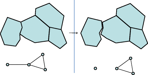

  

  Changing adjacency graph—edge of partition

  Fig. 9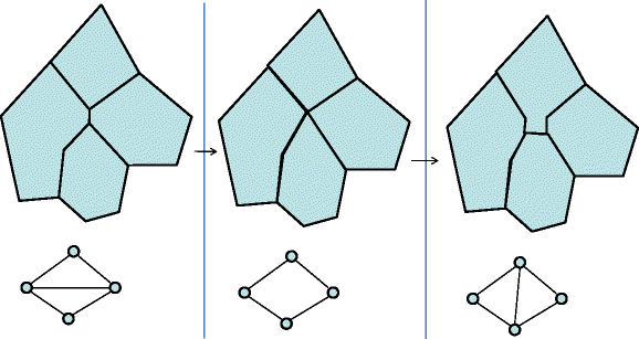

  

  changing Adjacency Graph—Inside Partition

• • Removing a node

  • ○ As nodes correspond to faces, this means that a face no longer exists. Insert a single point representing the face as a new version and interpolate neighbouring faces to this point. This point is the new meeting point of the eventual new cycle created by removing the node. All the edges from that node are also removed.

Adding an edge or node is just like removing one except that the process is reversed in time.

Whenever the adjacency graph is updated, all affected faces must have a new time slice, where the state at the beginning of this new time slice is the state according to UpdatePartitionInterpolation after the change in the graph.

5.2 Constructing a moving network

A network may consist either of nodes (points) with curves between them (like graphs except that the shape of the curves may be important) or routes and intersections. The difference between these two is that the routes-and-intersections model can be equivalent to a non-planar graph as routes may cross each other without intersecting (one road goes in a tunnel below another with no means of switching from one to the other).

If the entire network is updated at the same time instants, representing a changing network is trivial. A network unit is simply a collection of moving curves which end in the same moving points (nodes). Changes in topology (removal of edges or nodes, merging of nodes and edges) happen only between the time slices (at the end of one and beginning of the next) in this model.

When the curves are updated individually, they are interpolated as normal. Additionally, a new version of the end points is stored. The end points are interpolated in time between all the end points of all the curves that meet there. Thus the meeting point of four curves would be updated whenever any of the four curves is updated. This means that the final line segment of each curve changes more often than the other lines, and the interpolation of these line segments cannot use the normal algorithm. One alternative method would be this:

• Create the projection of the final line segments and the changing end point on a plane that is parallel to the time axis and has an angle to the x-y axis that is the average of the angle of the final line in the two snapshots. The time dimension must be converted into a spatial dimension and scaled so that the distances in space and time are similar in scale. The most important consideration is to create a triangulation to ensure that the moving curve is made up of planar facets despite the end point being updated more often than the rest of the curve.

• Create the Delaunay triangulation of the projected lines.

• Use this as the triangulation of the final line segments. Going back to a full 3D representation is easy since the triangulation does not insert any new points and the 3D coordinates of the points used are known.

One example of such a curve and the proposed interpolation algorithm is shown in Fig. 10.

Fig. 10

Interpolation of a line

For networks consisting of routes and intersections, a modified version of this method can be used. Each route is equivalent to a connected set of edges and each intersection is equivalent to a meeting point. Places where routes cross but there is no intersection are not represented as points. This is a simple way of distinguishing such crossings from regular intersections.

6 Handling current time

The database described so far handles historical spatiotemporal data quite well. However, when asked about the current state, it can only return the last state of the various polygons, and this state can be inconsistent for those polygons which have not been updated for some time. The following two subsections discuss two methods for handling current time:

6.1 Using the most recent version

This method bases its computations on the assumption that the objects have not changed their state too much since the last snapshot. If the objects are updated fairly frequently compared to how fast they change this method works well. However, if they change fast compared to how often they are updated the result would be highly inaccurate for an object that has not been updated in a while relatively to its pace of change. The method basically goes as follows:

• Take the most recent snapshot in the area of interest.

• Insert a new time slice of each object that extends from the last snapshot of the object to the current time. The object is considered to be static in this time slice.

• Remove parts of the new snapshots that are inside other objects. Always remove parts from the older objects as those are least reliable (the age of an object in this context is the age of the last snapshot).

• Add a buffer to the objects to eliminate cracks. Again: add a buffer to the oldest objects first. This buffer should be large enough that the region continues to border the same line segments that it bordered in its last snapshot.

This is a fairly simple method that works well in many cases. However, it does not take the movement of the objects into account and may therefore produce highly inaccurate results in cases in which the objects move fast.

6.2 Extrapolating the current state from past movement

The alternative to the last method is to try to extrapolate the shape of the object. This might be done using the following method:

• Take all the lines depicting the movement of points⁵ for all the objects and extend them to the current time.

• Remove the parts of the objects that are inside other objects using ordinary 2D intersection. Always remove from the older of the two objects as that is least reliable (the age of an object in this context is the age of the last snapshot). If the two objects are the same age, compute the average boundary.

• Add a buffer as described in the previous method.

Unlike the last method this method takes the movement of the objects into account and would be more accurate if it was not for one problem: It may cause consistency problems and weird boundaries as the points that make up the boundary move in different directions at different speeds. An example of this is shown in Fig. 11.

Fig. 11

Extrapolation using a triangle representation

The main problem here is that the interpolation method used in this paper, creating triangular facets from the boundary lines, is not good at extrapolation. If extrapolation is needed a different method should be used. If the main changes are to the position rather than the shape of the object, one could use a simple extrapolation in which the centre of the object continues to move as in the last snapshot while the shape is unchanged.

7 Implementation issues

In this section, several issues dealing with implementing this model are considered. To get the shape of a region in this model one would need to fetch the lines, curves and curve units that it consists of. Section 7.1 considers how to retrieve and update such collections in an efficient manner. Section 7.2 analyses the two methods presented in Section 7.1. Section 7.3 considers how one would compute temporal topological relationships like “Does object A enter object B” in our model.

7.1 Storing references or storing several copies of some objects

In this model many objects should have references to each other. For instance, the region object stores its boundary as a set of curve objects. This ensures consistency, but it also creates a problem. To fetch the geometry of a region, one must access all the curve objects that make up its boundary, and all the point objects that make up the meeting points for those curves. Unless these are stored together, this may slow down the system. Boundary curves cannot be stored together with both of the regions that they border as these regions may be stored in entirely different places on the disk. This is one of the reasons why, according to [22], so many GIS systems still use non-topological data structures.

An alternative is to store several copies of these objects. For the curve, one would store one copy for each of the two regions that have it as part of their boundaries. This would make retrieval more efficient, but would introduce the possibility of inconsistencies. To solve this one would need a database system that could handle integrity rules of the type “Objects A and B should always be equal”. This is similar to a foreign key constraint with cascading updates that many database systems already support. Such a system could then enforce this by always updating both curves when one is updated. This would require that each copy of the curve has a pointer to the other. This would increase the cost of updating as well as storage cost, but would reduce query costs.

This way of storing the model might be called the “twin storage model” to separate it from the original. That name is chosen because each curve unit may have a twin in another face unit. For a partition it would roughly double the storage space required. The geometry of the region takes up most of the storage space. The geometry of a region is stored in its boundary and all curve units that serve as the boundary between two regions are stored twice. For a line network storage space would only increase marginally as only the end points would have to be stored several times and the location of these is stored in the curve unit anyway as part of its geometry representation.

An overview of the twin storage mode is shown in a UML class diagram in Fig. 12. The composition notation from UML is used to show that objects of one class are stored inside objects of the other class. For face units many of the attributes have the cardinality [1..C]. This indicates that for each curve unit in the geometry there can be 0 or 1 twin references and 0 or 1 original curve references.

Fig. 12

Twin storage model

For many of the relationships, such as a point serving as an end point, the relationship is stored in only one object, typically the object for which the relationship has the lowest cardinality. This is common design practise in relational databases and helps to ensure consistency. However, one may choose to store the relationships both ways instead. This will increase storage cost as well as update cost to avoid inconsistencies, but may reduce query cost.

7.2 Costs for querying and updating the model using the twin model compared to storing objects separately

Consider the following three examples: Retrieving the geometry of a face at a particular time instant (query), adding a new time slice to the face (update), and correcting an error in the position of a point that makes up the geometry of a curve unit (update). The geometry of a face is stored in its curve units.

Fetching a face at a particular time—standard model: Retrieving a moving face at a given time in the basic model requires one index search and one disk access to retrieve the face object. We assume here that the face units of the face are stored with the face object. Then the curve units of the face unit need to be retrieved. If the curve unit file is also indexed with a spatial index (such as an R-tree), this requires one index search (with the bounding box of the face as the search area), and fetching all the curves returned by that search. Therefore fetching the shape of an uncertain face with the standard model requires two index searches and at least two disk accesses, possibly several as there are no guarantees that all the curve units of the region are stored together. Assuming an index height of four and that an average face unit consists of eight curve units this will take ${4}\left( {\text{index search}} \right) + {1}\left( {\text{retrieve face unit}} \right) + {4}\left( {\text{index search}} \right) + {8}\left( {\text{retrieve curve units}} \right) = {\text{17disk accesses}}$.

Adding a new time slice—standard model: To add a new time slice in the standard model one would have to fetch the last time slice of the region as well as that of neighbouring regions (since these might also need to be updated). This would require one index search and possibly several disk accesses to get the neighbours. After that new curve units would have to be constructed for the boundary curves of the updated region and stored along with existing curve units. This would require one index search (for the location at which they should be inserted) and disk writes to write the new curve units. Using the assumptions from the last paragraph and assuming that each face has four neighbours and therefore its boundary consists of four moving curves this will take ${4}\left( {\text{index search}} \right) + {1}\left( {\text{fetch region}} \right) + {4}\left( {\text{fetch neighbours}} \right) + {1}\left( {\text{write region}} \right) + {4}\left( {\text{write neighbours}} \right) + {4}\left( {\text{index search}} \right) + {8}\left( {\text{fetch curves}} \right) + {8}\left( {\text{write curves}} \right) = {\text{34 disk accesses}}$.

Fixing an error in a curve instant—standard model: To fix an error in a curve instant, one would need to fetch the two curve units that border this instant in time, and update them. Finding the two curve units would take one index search and possibly two disk reads if the curve units are in different disk blocks. Updating the curves would take one or two disk writes as the disk blocks containing the curves would have to be modified. Therefore this will take ${4}\left( {\text{index search}} \right) + {2}\left( {\text{fetch curve units}} \right) + {2}\left( {\text{write curve units}} \right) = {\text{8 disk accesses}}$.

Fetching a face at a particular time—twin storage model: In the twin storage model, the curve units are stored along with the face object. To get the geometry in this model would require one index search and one disk access to retrieve the face unit. The curve units are stored in the face units and require no additional time. As face units are larger in this storage model (since it stores the curve units) a face unit is assumed to take two disk blocks. This operation therefore takes ${4}\left( {\text{index search}} \right) + {2}\left( {\text{fetch face unit and component curves}} \right) = {\text{6 disk accesses}}$.

Adding a new time slice—twin storage model: Like in the standard model, the face unit that should be updated as well as its neighbours need to be fetched. After they are fetched new curve units are added to the face unit and its neighbours and written to disk, which would require one disk write for the face unit and one for each neighbour. Therefore this would take ${4}\left( {\text{index search}} \right) + {2}\left( {\text{fetch face}} \right) + {8}\left( {\text{fetch neighbours}} \right) + {2}\left( {\text{write face}} \right) + {8}\left( {\text{write neighbours}} \right) = {\text{24 disk accesses}}$.

Fixing an error in a curve instant—twin storage model: To fix an error in a curve instant one would have to find all objects that store that curve instant and update them. This becomes an index search for faces, an index search for curves and up to three writes, for a worst-case total of ${4}\left( {\text{face index search}} \right) + {4}\left( {\text{curve index search}} \right) + {5}\left( {\text{fetch two faces and a curve}} \right) + {5}\left( {\text{write the same objects}} \right) = {\text{18 disk accesses}}$.

Both fetching the geometry of a face and adding a new time slice to a face are considerable faster with the twin storage model than with the standard model using the assumptions given. Fixing errors in curve units is significantly faster in the standard model. Tests using the same formulas with different assumptions show that the ratios from Table 2 remain the same using different assumptions for fetching the geometry and fixing errors in curve units. This has been tested for differing index heights, number of neighbours of a face, number of curve units in a face unit and size of the face unit. For adding a new face time slice, the standard model becomes better if a face unit in the twin model takes four or more disk blocks. If the face has more then four neighbours or contains less than eight curve units, the standard model improves compared to the twin model for adding a new face to a time slice.

Table 2 Disk accesses for the example operations

7.3 Temporal topological predicates

Another implementation issue is determining the answers to temporal topological predicates, that is, predicates that indicate how the topological relationship between two objects change with time. Erwig and Schneider [16] defines two relationships as examples of temporal topological predicates:

• Enters: The object starts outside the region and moves inside it.

• Crosses: The object enters the region and later leaves it

The time slices in the hybrid model may be used to reduce the amount of data that needs to be fetched to do these computations. If each time slice has its own spatio-temporal bounding box, an index may be used to find those time slices of each object in which they may overlap. Then only those time slices need to be used to compute the temporal topology as for all other time slices the objects are known to be disjoint.

8 Summary

This paper has presented an extension to the sliced representation from [4] that is capable of representing explicit topology. This is necessary for several important operations, including checking whether two regions border each other. The new representation is somewhat more complex than the original representation, but many of the same algorithms are applicable to both. The main idea behind the representation is that time slices are good because they allow you to fetch only the temporal parts of the object that are interesting to you. However a slightly more general method for interpolating the object between snapshots than in [4] is necessary because neighbouring objects are not necessarily updated at the same time. Topology is maintained by having objects refer to one another and by storing geometry in the smallest object that uses it, the Curve Unit. Some algorithms for creating and updating this representation have been presented. Additionally an analysis of two different schemes for storing the representation has been presented and analysed: The original representation which represents topology by storing the geometry once and referring to it by all the objects that need it, and the twin storage model that stores the geometry with the objects and uses a system similar to foreign key constraints to ensure that geometry in several objects that is supposed to be the same really is the same.

References

Erwig M, Schneider M (1999) The honeycomb model for spatio-temporal partitions. In Proc. Int. Workshop on Spatio-Temporal Database Management, pp. 39–59
Worboys M (1995) GIS: a computing perspective. Taylor & Francis
van Oosterom P (1997) Maintaining consistent topology including historical data in a large spatial database. Auto Carto 13:327–336
Forlizzi L, Güting RH, Nardelli E, Schneider M (2000) A data model and data structures for moving objects databases. In Proc. ACM SIGMOD Int. Conf. on Management of Data (Dallas, Texas),pp. 319–330
Peuquet DJ (2001) Making space for time: issues in space-time data representation. GeoInformatica 5(1):11–32
Renolen A (1999) Concepts and methods for modelling temporal and spatiotemporal information. Dr. Ing Thesis, Norwegian University of Science and Technology (NTNU)
Peuquet DJ, Duan N (1995) An Event-based spatiotemporal data model (ESTDM) for temporal analysis of geographical data. Int J Geogr Inf Sci 9(1):7–24
Egenhofer MJ, Al-Taha KK (1992) Reasoning about gradual changes of topological relationships. In: Frank A, Campari I, Formentini U (eds) Theory and methods of spatio-temporal reasoning in geographic space, vol. 639 LNCS. Springer-Verlag, pp. 196–219
Güting RH, Schneider M (2005) Moving objects databases. Morgan Kaufmann
Koubarakis M, Sellis T et al (eds) (1998) Spatio-Temporal Databases, the CHOROCHRONOS approach. LNCS 2520, Springer-Verlag
Camossi E et al (2003) A multigranular spatiotemporal data model. In Proceedings of the 11th ACM international symposium on Advances in geographic information systems, pp. 94–101
Tøssebro E, Güting RH (2001) Creating representations for continuously moving regions from observations. In Proc. 7th Int. Symp. on Spatial and Temporal Databases, pp. 321–344
Hornsby K, Egenhofer MJ (2004) Modeling moving objects over multiple granularities. Ann Math Artif Intell 36(12)
Schneider M (2002) Implementing topological predicates for complex regions. In Proc. 10th Int. Symp. on Spatial Data Handling (SDH), pp. 313–328
Schneider M, Behr T (2006) Topological Relationships between Complex Spatial Objects. ACM Trans Database Syst 31(1):39–81
Erwig M, Schneider M (2002) Spatio-temporal predicates. IEEE Trans Knowl Data Eng (TKDE) 14(4):881–901
Egenhofer MJ, Franzosa RD (1991) Point-set topological spatial relations. Int J Geogr Inf Syst 5(2):161–174
Chomicki J, Revesz PZ (1999) A geometric framework for specifying spatiotemporal objects. In Proc. 6th Int. Workshop on Temporal Representation and Reasoning (TIME’99), pp. 41–46
Chomicki J, Revesz PZ (1997) Constraint-based interoperability of spatiotemporal databases. In Proc. 5th Int. Symp. on Large Spatial Databases, pp. 142–161
Grumbach S, Koubarakis M, Rigaux P, Scholl M, Skiadopoulos S (2003) Spatio-temporal models and languages: an approach based on constraints. In spatio-temporal databases—the CHOROCHRONOS approach, LNCS 2520, Springer-Verlag, pp. 177–201
Xie R, Shibasaki R (2005) A unified spatiotemproal schema for representing and querying moving feature. SIGMOD Rec 34(1):45–50
Theobald DM (2001) Topology revisited. Int J Geogr Inf Sci 15(8):689–705
Güting RH, Böhlen MF, Erwig M, Jensen CS, Lorentzos NA, Schneider M, Vazirgiannis M (2000) A foundation for representing and querying moving objects. ACM Trans Database Syst 25(1)
Ryden K (ed) OpenGIS Implementation Specification for Geographic Information—Simple feature access—Part 1: common architecture. OGC ref. no. 05-126
Boguslawski P, Gold C (2009) Construction operators for modelling 3D objects and dual navigation structures. In: Zlatanova S, Lee J (eds) Lecture notes in goinformation and cartography: 3d Geoinformation Sciences, Part II. Springer pp. 47–59
Open Access
This article is distributed under the terms of the Creative Commons Attribution Noncommercial License which permits any noncommercial use, distribution, and reproduction in any medium, provided the original author(s) and source are credited.
Author information
Authors and Affiliations
Corresponding author
Rights and permissions
Open Access This is an open access article distributed under the terms of the Creative Commons Attribution Noncommercial License (https://creativecommons.org/licenses/by-nc/2.0), which permits any noncommercial use, distribution, and reproduction in any medium, provided the original author(s) and source are credited.
About this article
Cite this article
Tøssebro, E., Nygård, M. Representing topological relationships for spatiotemporal objects. Geoinformatica 15, 633–661 (2011). https://doi.org/10.1007/s10707-010-0120-5
Received:
Revised:
Accepted:
Published:
Issue Date:
DOI: https://doi.org/10.1007/s10707-010-0120-5