
Abstract
Tillering is defined as the process of above-ground shoot production by a single plant. The number of grass tillers is one of the most important parameters in ecology and breeding studies. The number of tillers is usually determined by manually counting the separated shoots from a single plant. Unfortunately, this method is too time-consuming. In this study, a new method for counting grass tillers based on image analysis is presented. The usefulness of the method was evaluated for five grass species, Phleum pratense, Lolium perenne, Dactylis glomerata, Festuca pratensis and Bromus unioloides. The grass bunches were prepared for analysis by cutting and tip painting. The images obtained were analysed using an automatic procedure with separation of shoots and other objects based on morphological parameters. It was found that image analysis allows for very quick and accurate counting of grass tillers. However, the set of morphological parameters for object recognition must be selected individually for different grass species. This method can be recommended as a replacement for the traditional, time-consuming method in grass breeding.
Introduction
Variation in grass architecture (e.g. tillering, branching, leafage) profoundly affects light capture, competition and reproductive success and is responsive to environmental factors such as crowding and nutrients limitation. Linking environmental control of branching and tillering with specific modes of gene action might be the key to understanding genes via environmental interactions, and may provide a way to modify crop architecture to achieve greater yields (Doust 2007).
Tillering is defined as the process of above-ground shoot production by a single plant. The number of grass tillers is a characteristic for a particular species and varieties of plants and is usually determined by different environmental factors, such as soil parameters, climate, pathogens and pests (He et al. 2004; Kluse and Diaz 2005; Skalova 2010). Tillering ability determines the effectiveness in preventing soil losses and runoff (Hussein et al. 2007; Xiao et al. 2010).
The number of grass tillers is also an important parameter from the breeders’ point of view. Jeżowski (2008) reported that tillering and bunch diameter in the early stage of growing were the two most important traits influencing the biomass yield of Miscanthus clones. Tillering determination helps to identify high-yielding clones or varieties in the search for effective selection of grass hybrids during breeding. Plant tillering is also one of the main parameters which are commonly used in the determination of the stress tolerance of plants (Fernandez and Reynolds 2000; Kotanen and Bergelson 2000; Wachendorf et al. 2001). According to Głowacka et al. (2009), tillering is also a significant factor in judging the resistance of grasses to drought and low temperatures. Zimmermann et al. (2010) reported that reductions in light quality and quantity (also self-shading) were found to suppress the growth, initiation and survival of tillers.
Plant tillering is usually determined by manually counting separated shoots from a single plant. The main disadvantage of this method is that it is highly time-consuming. Calculating the tillering for a single grass plant with more than a hundred tillers usually takes couple of minutes. When the duration and precision of analyses are important, it seems that the application of image processing becomes a reasonable solution. In recent years, image analysis has been widely used for plant recognition, e.g. weed determination in precision agriculture. Selected species determination is based mainly on the characteristic colour and shape of the plant in question (Onyango et al. 2005; Søgaard 2005).
The purpose of this paper was to examine a new method of grass tillering determination based on image analysis and to evaluate the advantages and disadvantages of this method. This method was granted a patent by the Polish Patent Office in 2013 (No. 213091).
Methods
Plant material
The field experiment was conducted in Mydlniki near Krakow (50° 04′ N, 19° 51′ E) at the Institute of Machinery Exploitation, Ergonomics, and Production Processes, Agricultural University of Krakow, Poland, in the period from 2006 to 2008.
The seeds of five grass species (timothy-grass Phleum pratense L., perennial ryegrass Lolium perenne L., cocksfoot grass Dactylis glomerata L., meadow fescue Festuca pratensis L., prairie grass Bromus unioloides) were pre-sown in seed trays and then planted in the experimental field in 2006. A total number of 100 grass bunches, 20 bunches for each species, were prepared. The space between bunches was 0.6 m (in rows and between rows).
Grass tillering measurements
Measurements were conducted in 2007 and 2008. The tillering was determined during harvesting, three times a year. The tillering of particular grass bunches was determined using two methods: (i) the traditional method by manually counting separated shoots from a single bunch and (ii) image analysis of bunches after cutting. The second method occurred in three main stages: (i) preparing bunches for analysis, (ii) taking photos, and (iii) image analysis.
In the first stage, bunches of grass were cut with a mower, the best was a bar mower with the cutting height of 5 cm. Cut shoots were removed from the observation area.
At that stage, the shoot tips were painted with white acrylic paint. The paint was applied with a roller with the diameter of 3–5 cm. The scheme for grass bunches before and after cutting is presented in Fig. 1. Painting shoots white enables sharp, contrasting images of shoot tips to be taken, which helps with the precise separation of objects from their background.

Grass bunch before (a) and after (b) cutting. 1—grass stem cut at the 5 cm height, 2—white painting roller, 3—digital camera for capturing the image of the bunch
Image acquisition
In the second stage, the bunches were photographed. In the experiment, the images were collected using a Canon EOS 1000D camera (Canon Inc., Tokyo, Japan) (6.3 effective megapixels) with an EF 50 mm lens. The shutter speed was set at 1/500 s with a sensitivity of 200 ISO, autofocus, and automatic white balance setting. The photographed area was approximately 50 × 50 cm in size, covering the entire bunch of grass. Photos were taken at a distance of about 150 cm, with the camera perpendicular to the soil surface. Pictures were transferred to a computer and saved in JPG format at a resolution of 600 dpi.
Image processing
The third stage was a computer image analysis. The images were analysed using Aphelion Dev 4.2.0 software for image analysis (ADCIS S.A. and Amerinex Applied Imaging, Herouville Saint-Clair, France). The whole procedure of image analysis was subdivided into four main steps: filtering, segmentation, measurements and object separation (Wojnar and Majorek 1994). The following Aphelion functions were used to prepare this procedure:
-
(i)
ImgColorToRGB—the input image (Fig. 2a) is split into three bands: red (R), green (G) and blue (B). Since they offer the best contrast grey images based on the blue band were prepared for further processing (Fig. 2b).
Fig. 2 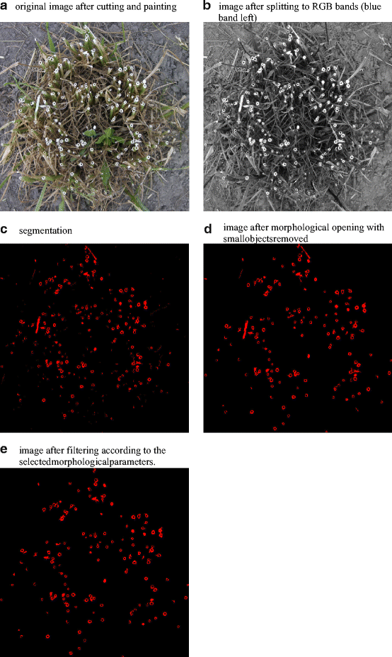
Flow diagram of the algorithm: a original image after cutting and painting; b image of the grass bunch after splitting to RGB bands (blue band left); c segmentation, red colour—object of interest, black colour—background; d image after morphological opening with small objects removed; e image after filtering according to the selected morphological parameters
-
(ii)
ImgMaximumContrastThreshold—this operator picks a set of thresholds that give maximal contrast. It automatically selects thresholds that maximize the global average contrast of edges detected by the thresholds across the image (Fig. 2c).
-
(iii)
ImgOpen—this operator performs a morphological opening on all the regions and it is used to remove objects smaller than 200 pixels (Fig. 2d).
-
(iv)
ObjComputeMeasurements—this is an operator which computes a variety of measurements (including shape parameters) for different spatial objects.

The following morphometric parameters were calculated:
-
(i)
A—area: the area of an object, expressed in pixel2
-
(ii)
SFcomp—compactness: shape factor that is calculated using the following Eq. (1):
-
(iii)
SFelong—elongation: the absolute value of the difference between the length of major (l max) and the minor axes (l min), divided by the sum of these lengths (Eq. 2). The minor axis is defined as the perpendicular axis to the major axis. This measure is zero for a circle and approaches 1 for a long, narrow ellipse.
-
(iv)
A conv—convex area: area of the convex hull (smallest shape that can completely contain an object such that, for any straight line segment connecting two points on the convex hull’s boundary, the entire line segment is contained inside the convex hull) of an object. A conv is always greater than or equal to A.
-
(v)
P conv—convex perimeter: perimeter of the convex hull of an object and expressed in calibrated units.
-
(vi)
SFconv—convexity: This is a measurement of the particle edge roughness and it is equal to the area of an object divided by the area of its convex hull, following Eq. (3):
-
(vii)
CMA—convex minimum angle: the minimum of the angles formed by the adjacent pairs of line segments that comprise the polygonal boundary of an object, given in radians.
-
(viii)
SMD—symmetry mean difference: mean of the absolute values of the length difference between the centroid (the arithmetic mean position of all the points in the shape) and two opposite boundary points of an object (l A and l A′). With N equal to the number of boundary points divided by two, the measurement’s formula is (Eq. 4):
-
(ix)
FDmax—maximum Feret diameter in an object’s set of Feret diameters
-
(x)
FDmin—minimum Feret diameter in an object’s set of Feret diameters
-
(xi)
SFsfer—Feret Pentland sphericity: shape factor introduced by Pentland (1927) (Eq. 5):
The calculated morphometric parameters cover the object’s dimensional features, such as area (A, A conv), perimeter (P conv, CMA) and diameter (FDmax, FDmin), expressed in calibrated units, as well as dimensionless shape factors (SFcomp, SFelong, SFconv, SMD, SFsfer).
Statistics
The basic statistics (number of measurements, mean, minimum and maximum values, and standard deviation) for data obtained by the two tested methods of tillering determination are presented in Table 1. Data were analysed using the statistical package Statistica v. 10.0 (StatSoft Inc., Tulsa, OK, USA).
Linear discriminant analysis (LDA) was used to classify the different objects based on their morphometric parameters. LDA is a technique commonly used to classify unknown groups characterized by quantitative and qualitative variables. A training set of objects used for parameter selection (approximately 1200 objects, 20 % of total number of objects) was divided into two classes: shoots and non-shoots. The parameters were selected on the basis of three statistical variables: tolerance, F-to-remove and Wilks’ lambda. The tolerance value indicates the proportion of a variable’s variance not accounted for by other independent variables in the model. F-to-remove values define the power of each variable in the model, and these are useful to describe what happens if a variable is removed from the current model. The values of the Wilks’ Lambda show the discriminatory ability of the LDA function.
The collinearity between the independent variables poses a statistical problem in regression models. The common diagnostic test for this is the variance inflation factor (VIF) (Zuur et al. 2010). Following the suggestion of Dormann et al. (2013), the VIF was computed and applied in a stepwise deletion of parameters according to decreasing VIF values, until a threshold of 10 was reached.
Regression models were determined when correlation coefficients were significant. The linear regression slope and intercept were tested for significant differences from 1 and 0, respectively, using an F test. The root mean square error (RMSE), mean absolute error (MAE), mean bias error (MBE) and coefficient of determination (R 2) were used to evaluate the accuracy of the implemented models and calculated as Eqs. 6, 7, 8 and 9:
where O i is the manually counted grass tillering, E i is the tillering estimated by image analysis, and n is the number of test data.
Results and discussion
The first problem, encountered during the procedure, was to distinguish the painted shoot tips from the background. The main components of the background are soil and grass leaves (living and thatch). Spectral analyses of soil show that all three bands (red, green and blue) are presented in equal proportions. It is a characteristic for soil that it has considerably fewer peak and valley variations in the reflectance (Langner et al. 2006). However, the reflectance of soil can vary depending on water and organic matter content. Picture quality is also affected by changes in illumination, which occur frequently due to changing weather, especially on partly cloudy days. A similar problem was also reported by Burgos-Artizzu et al. (2011). They recommended taking the pictures on cloudy days when the light is diffused and the contrast is lower. Plants show relatively low values in the red and the blue regions of the visible spectrum, with a peak in the green spectral band (Perez et al. 2000). Some colour indices based on the red, green and blue bands have been proposed to distinguish green leaves from soil as a background. Woebbecke et al. (1995) found that the excess green vegetation index 2G-R-B works well in the segmentation of vegetation against background. Meyer and Neto (2008) improved this index. They proposed an index based on excess green and red, which worked especially well for fresh wheat straw backgrounds. The normalized difference vegetation index (NDVI) recommended by Perez et al. (2000) uses only green and red channels (G-R)/(G + R). In this research, the blue band was chosen for further investigation according to Wiles (2011). This method was found to be sufficient to distinguish the region of interest. In this study, it was not necessary to use indices that are more complex. The separated tips of shoots were painted white, and it was much easier to distinguish them from the background than it would have been to separate all the green plants from the soil.
The next step in the procedure, after band splitting, was segmentation. The accuracy of segmentation depended on the difference between the objects (shoot tips) and their surroundings. In the image analysis of plant material, both automatic and manual segmentation are used. Automatic segmentation techniques have significantly developed in recent years (Sofou et al. 2001; Sezgin and Sankur 2004). Szala (2001) stated that, from the segmentation point of view, the best grey image should have two sets of pixels significantly different in grey level values. This was also confirmed by Wojnar et al. (2002) who indicated that automatic segmentation could be recommended for two maximum histograms, with clearly separated peaks. In this research, it was possible to use automatic segmentation (maximum contrast method) based on the histogram of the image. This method has also been used in weed detection (Philipp and Rath 2002). The result of the image analysis procedure was a set of objects. However, these objects presented not only the tips of grass shoots but also fragments of leaves and other debris. So, the next step in the image analysis procedure was filtration using morphological features of these objects.
Seven object parameters (out of 11) remained after performing the VIF stepwise method for deleting multi-collinear variables (Table 2). Grass species differ slightly in terms of the number of parameters which are included in LDA models (Table 3). All object parameters were used for recognition shoots of F. pratensis and L. perenne. Shoots of D. glomerata need six parameters, and for other species, five object parameters were included in the LDA model. Five parameters, namely CMA, SFcirc, SFconv, SFelong and SMD, were found to be very useful for all the investigated grass species. SFcirc had the best prediction value for D. glomerata and B. unioloides according to F-to-remove and Wilks’ lambda. SFelong had the most discriminant value for F. pratensis and L. perenne. The rest of the 11 proposed morphological parameters were found to be useless in the procedure of grass shoot tip recognition in bunch images.
The results present a good separation for shoot tips from the bunch images of all tested grass species. However, individual species need different sets of object morphological parameters. This can be ascribed to differences between tested grass species in terms of their shoot and leaf morphology. The investigated grass species differed in their vegetative stem shape and size. Both L. perenne and F. pratensis had round, thin stems with diameters up to 2 mm. The stem diameter for P. pratense, D. glomerata and B. unioloides was above 2 mm. The stem section shapes of P. pratense and B. unioloides were round, whereas the D. glomerata stem had a flattened base, which distinguished it from the other grasses. It was expected that for this species with flattened stems, there would be a problem with stem detection on the image and distinguishing them from cut leaves. However, this was not a significant problem, probably due to the small number of leaves at the cutting height. D. glomerata is a tall grass with a height up to 1.5 m, and in the lower part of the plants, there is low leafage. On the image obtained, there were not numerous leaf sections that could impede the analysis.
For image analysis of L. perenne, it was necessary to use more morphological parameters in comparison to other tested grasses. This species has dense leafage with numerous leaves on the lower part of the plant. The leaves are usually thin, with an area close to the diameter of the stem. The difficulty in counting stems using image analysis is connected with the problem of distinguishing stem sections and leaves on the images of bunches. P. pratense, with a round and thick stem and lower leafage on the lower parts of stem, needed only four morphological parameters to recognize the stem sections.
The parameters of linear regression for the relationships between the results for the number of grass tillers obtained by the two abovementioned methods are presented in Table 4. The results showed that all investigated grass species had a similar precision of tiller determination using the method based on image analysis. The value of the coefficients of determination, R 2, for the linear regression between the tested methods was 0.858 on average. The error indices for the linear regression, such as RMSA, MAE and MBA, also showed a high level of accuracy.
The main advantage of the described method is its speed of use. Preparing the bunch (painting) and taking the picture usually take several seconds per bunch, whereas counting stems in a bunch in the traditional method takes up to 5 min. In experiments with hundreds of bunches, this difference becomes very significant. However, it should be underlined that this method can be recommended only in breeding trials where separate bunches are cultivated and not in field trials with pasture mixtures and without weeds.
Conclusions
The use of image analysis enables very quick and accurate counting of grass tillers. This method could be recommended to replace the traditional, time-consuming method in grass breeding. The grass bunches should be sown separately and they must be prepared for analysis by cutting and tip painting. The images obtained can be analysed using an automatic procedure. Separation of shoot tips and other objects is based on morphological parameters. However, individual species need different sets of object morphological parameters which can be ascribed to differences in their shoot and leaf morphology. Further investigation is recommended in order to select the individual sets of morphological parameters for other grass species.
References
Burgos-Artizzu, X. P., Ribeiro, A., Guijarro, M., & Pajares, G. (2011). Real-time image processing for crop/weed discrimination in maize fields. Computers and Electronics in Agriculture, 75, 337–346.
Dormann, C. F., Elith, J., Bacher, S., Buchmann, C., Carl, G., Carré, G., Marquéz, J. R. G., Gruber, B., Lafourcade, B., Leitão, P. J., Münkemüller, T., McClean, C., Osborne, P. E., Reineking, B., Schröder, B., Skidmore, A. K., Zurell, D., & Lautenbach, S. (2013). Collinearity: a review of methods to deal with it and a simulation study evaluating their performance. Ecography, 36, 27–46.
Doust, A. N. (2007). Grass architecture: genetic and environmental control of branching. Current Opinion in Plant Biology, 10, 21–25.
Fernandez, R. J., & Reynolds, J. F. (2000). Potential growth and drought tolerance of eight desert grasses: lack of a Trade-off? Oecologia, 123, 90–98.
Głowacka, K., Jeżowski, S., & Kaczmarek, Z. (2009). Polyploidization of Miscanthus sinensis and Miscanthus x giganteus by plant colchicine treatment. Industrial Crops and Products, 30, 444–446.
He, W. M., Zhang, H., & Dong, M. (2004). Plasticity in fitness and fitness-related traits at ramet and genet levels in a tillering grass Panicum miliaceum under patchy soil nutrients. Plant Ecology, 172, 1–10.
Hussein, J., Yu, B., Ghadiri, H., & Rose, C. (2007). Prediction of surface flow hydrology and sediment retention upslope of a vetiver buffer strip. Journal of Hydrology, 338, 261–272.
Jeżowski, S. (2008). Yield traits of six clones of Miscanthus in the first 3 years following planting in Poland. Industrial Crops and Products, 27, 65–68.
Kluse, J. S., & Diaz, B. A. (2005). Importance of soil moisture and its interaction with competition and clipping for two montane meadow grasses. Plant Ecology, 176, 87–99.
Kotanen, P. M., & Bergelson, J. (2000). Effects of simulated grazing on different genotypes of Bouteloua gracilis: how important is morphology? Oecologia, 123, 66–74.
Langner, H. R., Bottger, H., & Schmidt, H. (2006). A special vegetation index for the weed detection in sensor based precision agriculture. Environmental Monitoring and Assessment, 117, 505–518.
Meyer, G. E., & Neto, J. C. (2008). Verification of color vegetation indices for automated crop imaging applications. Computers and Electronics in Agriculture, 63, 282–293.
Onyango, C., Marchant, J., Grundy, A., Phelps, K., & Reader, R. (2005). Image processing performance assessment using crop weed competition models. Precision Agriculture, 6, 183–192.
Pentland, A. (1927). A method of measuring the angularity of sands, Proceedings and Transactions of the Royal Society of Canada, 21.
Perez, A. J., Lopez, F., Benlloch, J. V., & Christensen, S. (2000). Colour and shape analysis techniques for weed detection in cereal fields. Computers and Electronics in Agriculture, 25, 197–212.
Philipp, I., & Rath, T. (2002). Improving plant discrimination in image processing by use of different colour space transformations. Computers and Electronics in Agriculture, 35, 1–15.
Sezgin, M., & Sankur, B. (2004). Survey over image thresholding techniques and quantitative performance evaluation. Journal of Electronic Imaging, 13(1), 146–165.
Skalova, H. (2010). Potential and constraints for grasses to cope with spatially heterogeneous radiation environments. Plant Ecology, 206, 115–125.
Sofou, A., Tzafestas, C., & Maragos, P. (2001). Segmentation of soil section images using connected operators. Proc. Int. Image Process., ICIP-2001, 1087–1090.
Søgaard, H. T. (2005). Weed classification by active shape models. Biosystems Engineering, 91(3), 271–281.
Szala, J. (2001). Application of computer image analysis into quantitative evaluation of material structure (in Polish). Gliwice: Silesia Polytechnics Press.
Wachendorf, M., Collins, R. P., Elgersma, A., Fothergill, M., Frankow-Lindberg, B. E., Ghesquiere, A., Guckert, A., Guinchard, M. P., Helgadottir, A., Luscher, A., Nolan, T., Nykanen-Kurki, P., Nosberger, J., Parente, G., Puzio, S., Rhodes, I., Robin, C., Ryan, A., Staheli, B., Stoffel, S., Taube, F., & Connolly, J. (2001). Overwintering and growing season dynamics of Trifolium repens L. in mixture with Lolium perenne L.: a model approach to plant-environment interactions. Annals of Botany, 88(Special Issue), 683–702.
Wiles, L. J. (2011). Software to quantify and map vegetative cover in fallow fields for weed management decisions. Computers and Electronics in Agriculture, 78, 106–115.
Woebbecke, D. M., Meyer, G. E., VonBargen, K., & Mortensen, D. A. (1995). Color indices for weed identification under various soil, residue and lighting conditions. Transactions of the ASAE, 38, 259–269.
Wojnar, L., & Majorek, M. (1994). Computer image analysis (in Polish). Cracow: Fotobit Design.
Wojnar, L., Kurzydłowski, K.J., & Szala, J. (2002). Practice of image analysis (in Polish). Polish Society for Stereology, Krakow.
Xiao, B., Wang, Q., Wu, J., Huang, C., & Yu, D. (2010). Protective function of narrow grass hedges on soil and water loss on sloping croplands in northern China. Agriculture, Ecosystems and Environment, 139, 653–664.
Zimmermann, J., Higgins, S. I., Grimma, V., Hoffmann, J., & Linstadter, A. (2010). Grass mortality in semi-arid savanna: the role of fire, competition and self-shading. Perspectives in Plant Ecology, Evolution and Systematics, 12, 1–8.
Zuur, A. F., Ieno, E. N., & Elphick, C. S. (2010). A protocol for data exploration to avoid common statistical problems. Methods in Ecology and Evolution, 1, 3–14.
Acknowledgments
Financial support for this study was provided by the Ministry of Science and Higher Education in Poland (statutory funds No. DS-3615/WIPiE/2014, Institute of Machinery Exploitation, Ergonomics and Production Processes, University of Agriculture in Krakow).
Author information
Authors and Affiliations
Corresponding author
Ethics declarations
Conflict of interest
The authors declare that they have no competing interests.
Rights and permissions
Open Access This article is distributed under the terms of the Creative Commons Attribution 4.0 International License (http://creativecommons.org/licenses/by/4.0/), which permits unrestricted use, distribution, and reproduction in any medium, provided you give appropriate credit to the original author(s) and the source, provide a link to the Creative Commons license, and indicate if changes were made.
About this article

Cite this article
Głąb, T., Sadowska, U. & Żabiński, A. Application of image analysis for grass tillering determination. Environ Monit Assess 187, 674 (2015). https://doi.org/10.1007/s10661-015-4899-2
Received:
Accepted:
Published:
DOI: https://doi.org/10.1007/s10661-015-4899-2