Potential Method in the Linear Theory of Viscoelastic Materials with Voids

Abstract

In the present paper the linear theory of viscoelasticity for Kelvin–Voigt materials with voids is considered and some basic results of the classical theory of elasticity are generalized. Indeed, the basic properties of plane harmonic waves are established. The explicit expression of fundamental solution of the system of equations of steady vibrations is constructed by means of elementary functions. The Green’s formulas in the considered theory are obtained. The uniqueness theorems of the internal and external basic boundary value problems (BVPs) are proved. The representation of Galerkin type solution is obtained and the completeness of this solution is established. The formulas of integral representations of Somigliana type of regular vector and regular (classical) solution are obtained. The Sommerfeld-Kupradze type radiation conditions are established. The basic properties of elastopotentials and singular integral operators are given. Finally, the existence theorems for classical solutions of the internal and external basic BVPs of steady vibrations are proved by using of the potential method (boundary integral method) and the theory of singular integral equations.

1 Introduction

The theories of viscoelasticity initiated by Maxwell, Meyer, Boltzmann, and studied by Voigt, Kelvin, Zaremba, Volterra and others. These theories, which include the Maxwell model, the Kelvin–Voigt model, and the standard linear solid model, were used to predict a material’s response under different loading conditions (see, Eringen [1], Truesdell and Noll [2], Christensen [3], Amendola et al. [4]).

Viscoelastic materials play an important role in many branches of civil engineering, geotechnical engineering, technology and, in recent years, biomechanics. Viscoelastic materials, such as amorphous polymers, semicrystalline polymers, and biopolymers, can be modeled in order to determine their stress or strain interactions as well as their temporal dependencies. Study of bone viscoelasticity is best placed in the context of strain levels and frequency components associated with normal activities and with applications of diagnostic tools (see, Lakes [5]). The investigations of the solutions of viscoelastic wave equations and the attenuation of seismic wave in the viscoelastic media are very important for geophysical prospecting technology. In addition, the behavior of viscoelastic porous materials can be understood and predicted in great detail using nano-mechanics. The applications of these materials are many. One of the applications may be to the NASA space program, such as the prediction of soils behavior in the Moon and Mars (for details, see, Voyiadjis and Song [6], Polarz and Smarsly [7], Chen et al. [8] and references therein).

A great attention has been paid to the theories taking into account the viscoelastic effects (see, Amendola et al. [4], Fabrizio and Morro [9], Di Paola and Zingales [10, 11]). The existence and the asymptotic stability of solutions in the linear theory of viscoelasticity for solids is investigated by Fabrizio and Lazzari [12], and Appleby et al. [13]. The main results on the free energy in the linear viscoelasticity are obtained in the series of papers [14–21]. A general way to provide existence of solutions of the initial and boundary value problems for linear viscoelastic bodies is provided without the need of appealing to transient solutions is presented by Fabrizio and Morro [9], Fabrizio and Lazzari [12], and Deseri et al. [14].

Material having small distributed voids may be called porous material or material with voids. The intended application of the theory of elastic material with voids may be found in geological materials like rocks and soils, in biological and manufactured porous materials for which the theory of elasticity is inadequate. But seismology represents only one of the many fields where the theories of elasticity and viscoelasticity of materials with voids is applied. Medicine, various branches of biology, the oil exploration industry and nanotechnology are other important fields of application.

Various theories of viscoelastic materials with voids of integral type have been proposed by Cowin [22], Ciarletta and Scalia [23], De Cicco and Nappa [24], and Martínez and Quintanilla [25]. In the last decade there are been interest in formulation of the mechanical theories of viscoelastic materials with voids of differential type. In this connection, Ieşan [26] has developed a nonlinear theory for a viscoelastic composite as a mixture of a porous elastic solid and a Kelvin–Voigt material. A linear variant of this theory was developed by Quintanilla [27], and existence and exponential decay of solutions are proved. Ieşan and Nappa [28] introduced a nonlinear theory of heat conducting mixtures where the individual components are modelled as Kelvin–Voigt viscoelastic materials. Some exponential decay estimates of solutions of equations of steady vibrations in the theory of viscoelastricity for Kelvin–Voigt materials are obtained by Chiriţă et al. [29]. A theory of thermoviscoelastic composites modelled as interacting Cosserat continua is presented by Ieşan [30].

In [31], Ieşan extends theory of elastic materials with voids (see, Nunziato and Cowin [32, 33]), the basic equations of the nonlinear theory of thermoviscoelasticity for “virgin”, namely in the absence pre-existing stresses (see, Fabrizio and Morro [9], Deseri et al. [13]), Kelvin–Voigt materials with voids are established, the linearized version of this theory is derived, a uniqueness result and the continuous dependence of solution upon the initial data and supply terms are proved. Recently, the theory of thermoviscoelasticity for Kelvin–Voigt microstretch composite materials is presented by Passarella et al. [34].

For a review of the literature on elastic materials with voids the reader is referred to [35–48] and the references therein. A new approach may be found in Amendola et al. [4], Fabrizio and Morro [9], although this is not limited just to voids. An account of the historical developments of the theory of porous media as well as references to various contributions may be found in the books by de Boer [49] and Ieşan [50].

In this paper the linear theory of viscoelasticity for Kelvin–Voigt materials with voids (see, Ieşan [31]) is considered and some basic results of the classical theory of elasticity are generalized. Indeed, the basic BVPs of steady vibrations are investigated using the potential method and the theory of singular integral equations.

The investigation of BVPs of mathematical physics by the classical potential method has a hundred year history. The application of this method to the 3D basic BVPs of the theory of elasticity reduces these problems to 2D singular integral equations (see, Kupradze et al. [51]). Owing to the works of Mikhlin [52], Kupradze [53], and Burchuladze and Gegelia [54], the theory of multidimensional singular integral equations has presently been worked out with sufficient completeness. An extensive review of works on the potential method can be found in Gegelia and Jentsch [55].

This work is articulated as follows. Section 2 is devoted to basic equations of steady vibrations of the linear theory of viscoelasticity for isotropic and homogeneous Kelvin–Voigt materials with voids with experienced no past strain histories prior of the instant of observation of the evolution of the body (see Ieşan [31]). The basis for generalizing the present analysis to pre-existing stresses may be found in [20, 21], where the state of the material is characterized for viscoelastic media. In Sect. 3 the basic properties of plane harmonic waves are established. In Sect. 4 the fundamental solution of the system of equations of steady vibrations is constructed by means of elementary functions, and its some basic properties are established. In Sect. 5 the Sommerfeld-Kupradze type radiation conditions are given and basic BVPs are formulated. In Sect. 6 the uniqueness theorems of these BVPs are proved. In Sect. 7 the Green’s formulas in the considered theory are obtained, the formulas of integral representations of Somigliana type of regular vector and regular (classical) solution are presented, the representation of Galerkin type solution is obtained and the completeness of this solution is established. In Sect. 8 the basic properties of the elastopotentials and the singular integral operators are given. Finally, in Sect. 9 the existence theorems of the BVPs of steady vibrations are proved.

On the basis of the potential method the uniqueness and existence theorems in the classical theories of viscoelasticity and thermoviscoelasticity for Kelvin–Voigt materials without voids are proved by Svanadze [56].

2 Basic Equations

We consider an isotropic homogeneous viscoelastic Kelvin–Voigt material with voids that occupies the region Ω of the Euclidean three-dimensional space R ³. Let x=(x ₁,x ₂,x ₃) be a point of R ³, $\mathbf{D}_{\mathbf{x}}=(\frac{\partial }{\partial x_{1}}, \frac{\partial}{\partial x_{2}}, \frac{\partial }{\partial x_{3}})$, and let t denote the time variable.

In the absence of the body force and the extrinsic equilibrated body force, the system of homogeneous equations of motion in the linear theory of viscoelasticity for Kelvin–Voigt materials with voids has the following form (see, Ieşan [31])

(2.1)

where $\mathbf{u}'=(u'_{1}, u'_{2}, u'_{3})$ is the displacement vector, φ′ is the volume fraction field, ρ is the reference mass density (ρ>0), ρ ₀=ρκ,κ is the equilibrated inertia (κ>0); λ,μ,b,α,ξ, λ ^∗,μ ^∗,b ^∗,α ^∗,ν ^∗,ξ ^∗ are the constitutive coefficients, and a superposed dot denotes differentiation with respect to $t: \dot{\mathbf{u}}'=\frac{\partial\mathbf{u}'}{\partial t}, \ddot{\mathbf{u}}'=\frac {\partial^{2} \mathbf{u}'}{\partial t^{2}}$.

The system (2.1) we can rewritten as

(2.2)

where

(2.3)

If the displacement vector u′ and the volume fraction function φ′ are postulated to have a harmonic time variation, that is,

then from system of equations of motion (2.2) we obtain the following system of homogeneous equations of steady vibrations

(2.4)

where ω is the oscillation frequency (ω>0),

(2.5)

Obviously, (2.4) is the system of partial differential equations with complex coefficients in with are 14 real parameters: λ,λ ^∗,μ,μ ^∗,b,b ^∗,α,α ^∗,ξ,ξ ^∗,ν ^∗,ω,ρ and ρ ₀.

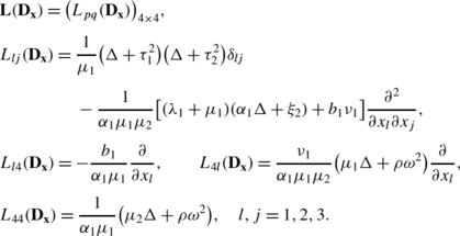
We introduce the matrix differential operator

where δ _lj is the Kronecker delta, and l,j=1,2,3. The system (2.4) can be written as

(2.6)

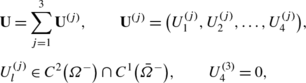
where U=(u,φ) and x∈Ω.

On the other hand the system of nonhomogeneous equations of steady vibrations in the linear theory of viscoelastic materials with voids can be written as follows

(2.7)

where F′ and s are is the body force and the extrinsic equilibrated body force per unit mass, respectively. The system (2.7) can be written as

(2.8)

where F=(−ρ F′,−ρs).

Throughout this article, we suggest that ξ ₂≠0 (the case ξ ₂=0 is to simple to be considered).

3 Plane Harmonic Waves

We introduce the notation

(3.1)

In this section, it is assumed that

(3.2)

On the basis of (3.2) from (3.1) we get

(3.3)

Suppose that plane harmonic waves corresponding to the wave number τ and angular frequency ω are propagated in the x ₁-direction through the viscoelastic Kelvin–Voigt material with voids. Then

(3.4)

where B=(B ₁,B ₂,B ₃); B ₀,B ₁,B ₂ and B ₃ are constants.

Keeping in mind (2.3) and (3.4) from (2.2) it follows that

(3.5)

From (3.5) for B ₀ and B ₁ we have

(3.6)

For the system (3.6) to have a non-trivial solution for B ₀ and B ₁ we must set the determinant of their coefficients equal to zero, thus

(3.7)

In the same way from (3.5) for B ₂ and B ₃ we have

(3.8)

and if τ is the solution of equation

(3.9)

then (3.8) have non-trivial solution.

The relations (3.7) and (3.9) will be called the dispersion equations of longitudinal and transverse plane waves in the linear theory of viscoelasticity for Kelvin–Voigt materials with voids, respectively. It is obvious that if τ>0, then the corresponding plane wave has the constant amplitude, and if τ is complex with $\operatorname{Im}\tau>0$, then the plane wave is attenuated as x ₁→+∞.

Let $\tau_{1}^{2}$, $\tau_{2}^{2}$ and $\tau_{3}^{2}$ be roots of (3.7) and (3.9) with respect to τ ², respectively. Obviously,

One may easily verify that $\tau_{3}^{2}$ is a complex number. Obviously, τ ₁, τ ₂ and τ ₃ are the wave numbers of longitudinal and transverse plane harmonic waves, respectively.

We denote the longitudinal plane wave with wave number τ _j (j=1,2) by P _j (P-primary), and the transverse horizontal and vertical plane waves with wave number τ ₃ by SH and SV, respectively (S-secondary, see Achenbach [57]).

Lemma 3.1

If the conditions (3.2) are satisfied, then (3.7) with respect to τ ² has not a positive root.

Proof

Let η be a real root of the equation

(3.10)

Separating real and imaginary parts in (3.10), on the basis of (2.5), (3.1) and equalities

we obtain the following system

(3.11)

As one may easily verify, the system (3.11) may be written in the form

(3.12)

(3.13)

where η ₁=μ ₀ η−ρω ²,η ₂=αη−ξ ₀. Obviously, by (3.12) and (3.13) we have ηη ₂≠0. Taking into account (3.12) from (3.13) it follows that

and hence,

(3.14)

where

By virtue of conditions (3.2) and (3.3) we have

Therefore from (3.14) we obtain η(η−η ₀)<0. Finally, we may write η∈ ]η ₀;0[ and Lemma 3.1 is thereby proved. □

We assume that $\operatorname{Im}\tau_{j}>0\ (j=1,2,3)$. Lemma 3.1 leads to the following result.

Theorem 3.1

If the conditions (3.2) are satisfied, then through a Kelvin–Voigt material with voids 4 plane harmonic plane waves propagate: two longitudinal plane waves P ₁ and P ₂ with wave numbers λ ₁,λ ₂ and two transverse plane waves SH and SV with wave number λ ₃; these are attenuated waves as x ₁→+∞.

Remark 3.1

It is obvious that if plane harmonic waves are propagated in an arbitrary direction through a Kelvin–Voigt material with voids, then we obtain the same result as given in Theorem 3.1.

4 Fundamental Solution

In what follows we assume that $\tau_{1}^{2}\ne\tau_{2}^{2}\ne\tau_{3}^{2}\ne\tau_{1}^{2}$. In the sequel we use the matrix differential operators:

• (1)
  

  (4.1)
• (2)
  

  (4.2)

We have the following result.

Lemma 4.1

If

(4.3)

then

(4.4)

Lemma 4.1 is proved by direct calculation.

We introduce the notations

where

Obviously, Y is the fundamental matrix of operator Λ, that is,

(4.5)

where δ(x) is the Dirac delta, J=(δ _pq )_4×4 is the unit matrix, and x∈R ³.

We define the matrix Γ=(Γ _pq )_4×4 by

(4.6)

In view of (4.4)–(4.6) we get

Hence, Γ( x ) is the fundamental matrix of differential operator A(D _x ). We have thereby proved the following theorem.

Theorem 4.1

If condition (4.3) is satisfied, then the matrix Γ(x) defined by (4.6) is the fundamental solution of system (2.4).

We are now in a position to establish basic properties of matrix Γ(x). Theorem 4.1 leads to the following results.

Corollary 4.1

If condition (4.3) is satisfied, then each column of the matrix Γ(x) is the solution of the homogeneous equation (2.6) at every point x∈R ³ except the origin.

Corollary 4.2

If condition (4.3) is satisfied, then the fundamental solution of the system

is the matrix Ψ=(Ψ _pq )_4×4, where

Clearly (see, Kupradze et al. [51]), the relations

hold in a neighborhood of the origin.

On the basis of Theorem 4.1 and Corollary 4.2 we obtain the following result.

Theorem 4.2

If condition (4.3) is satisfied, then the relations

hold in a neighborhood of the origin, where m=m ₁+m ₂+m ₃,m≥1,m _l ≥0,l=1,2,3 and p,q=1,2,3,4.

Thus, Ψ(x) is the singular part of the fundamental matrix Γ(x) in the neighborhood of the origin.

5 Radiation Conditions. Basic Boundary Value Problems

Let S be the smooth closed surface surrounding the finite domain Ω ⁺ in $R^{3}, \bar{\varOmega}^{+}=\varOmega^{+}\cup S, \varOmega^{-} =R^{3}\backslash \bar{\varOmega}^{+}, \bar{\varOmega}^{-}=\varOmega^{-}\cup S$. The scalar product of two vectors w=(w ₁,w ₂,…,w _l ) and v=(v ₁,v ₂,…,v _l ) is denoted by $\mathbf{w}\cdot\mathbf{v}=\sum^{l}_{j=1}w_{j}\bar{v}_{j}$, where $\bar{v}_{j}$ is the complex conjugate of v _j .

Definition 5.1

A vector function U=(u,φ)=(U ₁,U ₂,U ₃,U ₄) is called regular in Ω ⁻ (or Ω ⁺) if

• (1)
  
• (2)
  
• (3)
  

  (5.1)

  and

  

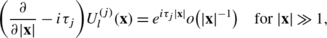
  (5.2)

  where j=1,2,3,l=1,2,3,4.

Equalities in (5.2) are the Sommerfeld-Kupradze type radiation conditions in the linear theory of viscoelasticity for materials with voids (see, Sommerfeld [58], Kupradze [59]). We note that (5.1) and (5.2) imply (for details see, Vekua [60])

(5.3)

It is easy to see that each column of the matrix Γ(x) is a regular vector in the domains Ω ⁺ and Ω ⁻. Indeed, each element of the matrix Γ(x) satisfies the radiation conditions (5.2) and (5.3).

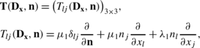
In the sequel we use the matrix differential operators

• (1)
  
• (2)
  
• (3)
  

  where n=(n ₁,n ₂,n ₃) is the unit vector, $\frac {\partial}{\partial\mathbf{n}}$ is the derivative along the vector n and l,j=1,2,3.

The basic internal and external BVPs of steady vibration in the theory of viscoelastic materials with voids are formulated as follows.

Find a regular (classical) solution to system (2.8) for x∈Ω ⁺ satisfying the boundary condition

(5.4)

in the Problem $(I)_{\mathbf{F,f}}^{+}$,

(5.5)

in the Problem $(\mathit{II})_{\mathbf{F,f}}^{+}$.

Find a regular (classical) solution to system (2.8) for x∈Ω ⁻ satisfying the boundary condition

(5.6)

in the Problem $(I)_{\mathbf{F,f}}^{-}$, and

(5.7)

in the Problem $(\mathit{II})_{\mathbf{F,f}}^{-}$. Here F and f are the known four-component vector functions, $\operatorname{supp} \mathbf{F}$ is a finite domain in Ω ⁻, and $\mathbf{n(z)}$ is the external (with respect to Ω ⁺) unit normal vector to S at z.

6 Uniqueness Theorems

In this section we prove uniqueness of regular solutions of BVPs $(K)_{\mathbf{F,f}}^{+}$ and $(K)_{\mathbf{F,f}}^{-}$, where K=I,II.

Theorem 6.1

If conditions

(6.1)

are satisfied, then the internal BVP $(K)_{\mathbf{F,f}}^{+}$ admits at most one regular solution, where K=I,II.

Proof

Suppose that there are two regular solutions of problem $(K)_{\mathbf{F,f}}^{+}$. Then their difference U corresponds to zero data $(\mathbf{F=f=0})$, i.e., U is a regular solution of problem $(K)_{{\bf0,0}}^{+}$.

On account of (2.4) from Green’s formulas (see, Kupradze et al. [51])

and identity

it follows that

(6.2)

where

Clearly, W ⁽¹⁾(u,λ ₁,μ ₁)=W ⁽¹⁾(u,λ,μ)−iωW ⁽¹⁾(u,λ ^∗,μ ^∗). In view of (6.2) we get

(6.3)

On the basis of homogeneous boundary condition and the identity

we obtain from (6.3)

(6.4)

Obviously, with the help of (6.1) it follows that

and from (6.4) we have

It is easy to verify that the last equation leads to the following relations

(6.5)

for x∈Ω ⁺. In view of (6.5) we get W ⁽¹⁾(u,λ,μ)=0 and W ⁽¹⁾(u,λ ^∗,μ ^∗)=0. Hence, W ⁽¹⁾(u,λ ₁,μ ₁)=0. Finally, from (6.3) we obtain $\mathbf{u(x)=0}$. Thus, $\mathbf{U(x)=0}$ for x∈Ω ⁺. □

Lemma 6.1

If U=(u,φ)∈C ²(Ω) is a solution of the system (2.4) for x∈Ω, then

(6.6)

where Ω is an arbitrary domain in R ³, u ^(j) and φ ^(l) satisfy the following equations

(6.7)

Proof

Applying the operator $\operatorname{div}$ to the first equation of (2.4) we get

(6.8)

Clearly, from system (6.8) we have

(6.9)

Now, applying the operator $(\Delta+\tau_{1}^{2}) (\Delta+\tau_{2}^{2})$ to the first equation of (2.4) and using (6.9) we obtain

(6.10)

We introduce the notation

(6.11)

By virtue of (6.9) and (6.10) the relations (6.6) and (6.7) can be easily obtained from (6.11). □

Now let us establish the uniqueness of a regular solution of external BVPs.

Theorem 6.2

If conditions (6.1) are satisfied, then the external BVP $(K)_{\mathbf{F,f}}^{-}$ admits at most one regular solution, where K=I,II.

Proof

Suppose that there are two regular solutions of problem $(K)_{\mathbf{F,f}}^{-}$. Then their difference U corresponds to zero data $(\mathbf{F=f=0})$, i.e., U is a regular solution of the problem $(K)_{{\bf0,0}}^{-}$.

Let $\varOmega_{\it r}$ be a sphere of sufficiently large radius ${\it r}$ so that $\bar{\varOmega}^{+}\subset\varOmega_{\it r}$. By virtue of homogeneous boundary condition $(\mathbf{f=0})$, the formula (6.3) for the domain $\varOmega_{\it r}^{-}=\varOmega^{-}\cap\varOmega_{\it r}$ can be rewritten as

(6.12)

where S _r is the boundary of the sphere Ω _r . From (6.12) we have

(6.13)

where

(6.14)

Obviously, by condition (6.1) it follows from (6.14) that N≥0.

On the other hand, keeping in mind the radiation conditions (5.3) from (6.6) we obtain

(6.15)

where $\tau_{0}={\rm min} \{ \operatorname{Im} \tau_{1}, \operatorname{Im} \tau_{2}, \operatorname{Im} \tau_{3}\}>0$. On account of conditions (5.2), (5.3) and (6.15) from (6.13) it follows that N=0. Hence, from (6.14) we get

(6.16)

Quite similarly as in Theorem 6.1 on the basis of (6.1) from (6.16) we obtain $\mathbf{U(x)=0}$ for x∈Ω ⁻. □

7 Green’s Formulas. Representations of General Solutions

In this section, first, we establish the Green’s formulas in the linear theory of viscoelastic materials with voids, then we obtain the integral representation of regular vector (representation of Somigliana-type) and the Galerkin-type solution of the system (2.8), and finally, we establish the representation of the general solution of the system of homogeneous equations (2.4) by solutions of Helmholtz equations (metaharmonic functions).

In the sequel we use the matrix differential operators $\tilde{\mathbf{A}}(\mathbf{D}_{\mathbf{x}})$ and $\tilde{\mathbf{P}}(\mathbf{D}_{\mathbf{x}}, \mathbf{n})$, where

and the superscript ⊤ denotes transposition.

Obviously, the fundamental matrix $\tilde{\boldsymbol{\Gamma}}(\mathbf{x})$ of operator $\tilde{\mathbf{A}}(\mathbf{D}_{\mathbf{x}})$ satisfies the following condition

(7.1)

Let $\tilde{\mathbf{U}}_{j}$ be the j-th column of the matrix $\tilde{\mathbf{U}}=(\tilde{U}_{lj})_{4\times4}, j=1,2,3,4$. As in classical theory of thermoelasticity (see, for details Kupradze et al. [49]) we can prove the following result.

Theorem 7.1

If U and $\tilde{U}_{j} (j=1,2,3,4)$ are regular vectors in Ω ⁺, then

(7.2)

On the basis of Theorem 7.1 and radiation conditions (5.2) we obtain the following result.

Theorem 7.2

If U and $\tilde{U}_{j} \ (j=1,2,3,4)$ are regular vectors in Ω ⁻, then

(7.3)

The identities (7.2) and (7.3) are the Green’s formulas in the linear theory of viscoelastic materials with voids for domains Ω ⁺ and Ω ⁻, respectively.

Keeping in mind (7.1) from (7.2) and (7.3) we obtain the formulas of integral representation of regular vector (representation of Somigliana-type) for the domains Ω ⁺ and Ω ⁻.

Theorem 7.3

If U is a regular vector in Ω ⁺, then

(7.4)

Theorem 7.4

If U is a regular vector in Ω ⁻, then

(7.5)

The next two theorems provide a Galerkin-type solution to system (2.8).

Theorem 7.5

Let

(7.6)

where w=(w ₁,w ₂,w ₃)∈C ⁶(Ω),w ₀∈C ⁴(Ω), and

(7.7)

Then, U=(u,φ) is a solution of system (2.8).

Proof

By virtue of (4.1) and (4.2), (7.7) and (7.7) we can rewrite in the form

(7.8)

and

(7.9)

respectively, where W=(w,w ₀). Clearly, by (4.4), (7.8) and (7.9) the vector U is a solution of the system (2.8). □

Theorem 7.6

If U=(u,φ) is a solution of system (2.8) in Ω, then U is represented by (7.8), where W=(w,w ₀) is a solution of (7.9) and Ω is a finite domain in R ³.

Proof

Let U be a solution of system (2.8). Obviously, if Ψ′(x) is the fundamental matrix of the operator L(D _x ), then the vector function

is a solution of (7.8).

On the other hand, by virtue of (2.8), (4.4) and (7.8) we have

Hence, W is a solution of (7.9). □

Remark 7.1

Quite similarly as in Theorem 4.1 we can construct the fundamental matrix Ψ′(x) of the operator L(D _x ) by elementary functions.

Thus, on the basis of Theorems 7.5 and 7.6 the completeness of Galerkin-type solution of system (2.8) is proved.

Now we consider the system of homogeneous equations (2.4). We have the following results.

Theorem 7.7

If metaharmonic function φ _j and metaharmonic vector function ψ=(ψ ₁,ψ ₂,ψ ₃) are solutions of equations

(7.10)

and

(7.11)

respectively, then U=(u,φ) is a solution of the homogeneous equation (2.4), where

(7.12)

for x∈Ω;Ω is an arbitrary domain in R ³ and

(7.13)

Proof

Keeping in mind the relations (7.10)–(7.13) and

we obtain by direct calculation

Quite similarly, by virtue of (7.12), (7.13) and

we have

 □

Theorem 7.8

If U=(u,φ) is a solution of the homogeneous equation (2.4) in Ω, then U is represented by (7.12), where φ _j and ψ=(ψ ₁,ψ ₂,ψ ₃) are solutions of (7.10) and (7.11), respectively; Ω is an arbitrary domain in R ³ and c _j (j=1,2) is given by (7.13).

Proof

Applying the operator div to the first equation of (2.4), from system (2.4) we have

(7.14)

Clearly, we obtain from (7.14)

(7.15)

Now applying the operator curl to the first equation of (2.4) it follows that

(7.16)

We introduce the notation

(7.17)

Taking into account (7.15)–(7.17), the function φ _j and vector function ψ are the solutions of (7.10) and (7.11), respectively, and the function φ is represented by (7.12).

Now we prove the first relation of (7.12). Obviously, on the basis of (7.10) we may rewrite the second equation of (7.14) in the form

(7.18)

where

Keeping in mind (7.17), (7.18) and identity

from (2.4) we obtain

(7.19)

Finally, from (7.19) we get the first relation of (7.12). □

Hence, on the basis of Theorems 7.7 and 7.8 the completeness of solution of the homogeneous equation (2.4) is proved.

8 Basic Properties of Elastopotentials

On the basis of a Somigliana-type integral representation of a regular vector (see, (7.4)) we introduce the following notations

where g and ϕ are four-component vectors.

As in the classical theory of elasticity (see, e.g., Kupradze et al. [51]), the vector functions $\mathbf{Z}^{(1)}{\bf(x,g)}$, $\mathbf{Z}^{(2)}{\bf(x,g)}$ and Z ⁽³⁾(x,ϕ,Ω ^±) are called a single-layer, a double-layer and volume potentials in the linear theory of viscoelasticity for Kelvin–Voigt materials with voids, respectively.

Obviously, on the basis of (7.4) and (7.5), the regular vector in Ω ⁺ and Ω ⁻ is represented by the sum of the elastopotentials as follows

and

respectively.

First we establish the basic properties of elastopotentials.

Theorem 8.1

If S∈C ^m+1,p,g∈C ^m,p′(S),0<p′<p≤1, and m is a non-negative integer, then:

• (a)
  
• (b)
  
• (c)
  

  (8.1)
• (d)
  

  is a singular integral, for z∈S.

Theorem 8.2

If S∈C ^m+1,p,g∈C ^m,p′(S),0<p′<p≤1, then:

• (a)
  
• (b)
  
• (c)
  

  (8.2)

  for the non-negative integer m,

• (d)
  

  is a singular integral, for z∈S,

• (e)
  

  for the natural number m and z∈S.

Theorem 8.3

If S∈C ^1,p,ϕ∈C ^0,p′(Ω ⁺),0<p′<p≤1, then:

• (a)
  
• (b)
  

  where $\varOmega_{0}^{+}$ is a domain in R ³ and $\varOmega_{0}^{+}\subset \varOmega^{+}$.

Theorem 8.4

If $S\in C^{1,p}, \operatorname{supp} {\boldsymbol{\phi}}= \varOmega\subset\varOmega^{-}, {\boldsymbol{\phi}}\in C^{0,p '}(\varOmega^{-}), 0<p'<p\le1$, then:

• (a)
  
• (b)
  

  where Ω is a finite domain in R ³ and $\bar{\varOmega}_{0}^{-} \subset\varOmega^{-}$.

Theorems 8.1 to 8.4 can be proved similarly to the corresponding theorems in the classical theory of thermoelasticity (for details, see, Kupradze et al. [51], Chap. X).

We introduce the notation

(8.3)

where ζ is a complex parameter. On the basis of Theorems 8.1 and 8.2, $\mathcal{K}^{(j)} \ (j=1,2,3,4)$ and $\mathcal{K}_{\zeta}$ are singular integral operators (for the definition a singular integral operator see, e.g., Mikhlin [52]).

In the sequel we need the following Lemmas.

Lemma 8.1

If conditions (6.1) are satisfied, then the singular integral operators $\mathcal{K}^{(j)} (j=1,2,3,4)$ are of the normal type.

Proof

Let ${\boldsymbol{\sigma}}^{(j)}=(\sigma_{lm}^{(j)})_{4\times4}$ be the symbol of the singular integral operator $\mathcal{K}^{(j)} (j=1,2,3.4)$ (see, e.g., Mikhlin [52]). Taking into account (8.3) we find (for details, see, Kupradze et al. [51], Chap. IV)

(8.4)

Keeping in mind the relations (6.1), from (8.4) we have

(8.5)

Hence, the operator $\mathcal{K}^{(j)}$ is of the normal type, where j=1,2,3,4. □

Lemma 8.2

If $\mathcal{L}$ is a continuous curve on the complex plane connecting the origin with the point ζ ₀ and $\mathcal{K}_{\zeta}$ is a normal type operator for any $\zeta\in\mathcal{L}$, then the index of the operator $\mathcal{K}_{\zeta_{0}}$ vanishes, i.e.,

Lemma 8.2 is proved in Kupradze et al. [51], Chap. IV.

Lemma 8.3

If conditions (6.1) are satisfied, then the Fredholm’s theorems are valid for the singular integral operator $\mathcal{K}^{(j)}$ ($\mathcal{K}^{(j)}$ is Fredholmian), where j=1,2,3,4.

Proof

Let σ _ζ and $\operatorname{ind} \mathcal{K}_{\zeta}$ be the symbol and the index of the operator $\mathcal{K}_{\zeta}$, respectively. It may be easily shown that

and $\operatorname{det} {\boldsymbol{\sigma}}_{\zeta}$ vanishes only at two points ζ ₁ and ζ ₂ of the complex plane. By virtue of (8.5) and $\operatorname{det} {\boldsymbol{\sigma}}_{1}=\operatorname{det} {\boldsymbol{\sigma}}^{(1)}$ we get ζ _j ≠1 for j=1,2. By Lemma 8.2 we obtain

Equation $\operatorname{ind} \mathcal{K}^{(2)}=0$ is proved in a quite similar manner. Obviously, the operators $\mathcal{K}^{(3)}$ and $\mathcal{K}^{(4)}$ are the adjoint operators for $\mathcal{K}^{(2)}$ and $\mathcal{K}^{(1)}$, respectively. Evidently,

Thus, the singular integral operator $\mathcal{K}^{(j)}\ (j=1,2,3,4)$ is of the normal type with an index equal to zero. Consequently, the Fredholm’s theorems are valid for $\mathcal{K}^{(j)}$ (for details, see, e.g., Mikhlin [52]). □

Remark 8.1

The definitions of a normal type singular integral operator, the symbol and the index of operator are given in Kupradze et al. [51] and Mikhlin [52].

9 Existence Theorems

Obviously, by Theorems 8.3 and 8.4 the volume potential $\mathbf{Z}^{(3)}(\mathbf{x,F},\varOmega^{\pm})$ is a regular solution of (2.8), where $\mathbf{F}\in C^{0,p '}(\varOmega^{\pm}), 0<p'\le1; \operatorname{supp} \mathbf{F}$ is a finite domain in Ω ⁻. Therefore, further we will consider problem $(K)_{{\bf0,f}}^{\pm}$ for K=I,II. In addition, we assume that the conditions (6.1) are satisfied.

Now we prove the existence theorems of a regular (classical) solution of problems $(K)_{{\bf0,f}}^{+}$ and $(K)_{{\bf0,f}}^{-}$ for K=I,II.

Problem $(I)_{{\bf0,f}}^{+}$: We seek a regular solution to problem $(I)_{{\bf0,f}}^{+}$ in the form

(9.1)

where g is the required four-component vector function.

By Theorem 8.2 the vector function U is a solution of (2.6) for x∈Ω ⁺. Keeping in mind the boundary condition (5.4) and using (8.2), from (9.1) we obtain, for determining the unknown vector g, a singular integral equation

(9.2)

By Lemma 8.3 the Fredholm’s theorems are valid for operator $\mathcal{K}^{(1)}$. We prove that (9.2) is always solvable for an arbitrary vector f. Let us consider the associate homogeneous equation

(9.3)

where h ₀ is the required four-component vector function. Now we prove that (9.3) has only the trivial solution.

Indeed, let h ₀ be a solution of the homogeneous equation (9.3). On the basis of Theorem 8.1 and (9.3) the vector function $\mathbf{V(x)}=\mathbf{Z}^{(1)}(\mathbf{x,h}_{0})$ is a regular solution of problem $(\mathit{II})_{{\bf0,0}}^{-}$. Using Theorem 6.2, the problem $(\mathit{II})^{-}_{\mathbf{0,0}}$ has only the trivial solution, that is

(9.4)

On other hand, by Theorem 8.1 and (9.4) we get

i.e., the vector $\mathbf{V(x)}$ is a regular solution of problem $(I)_{{\bf0,0}}^{+}$. Using Theorem 6.1, the problem $(I)^{+}_{{\bf0,0}}$ has only the trivial solution, that is,

(9.5)

By virtue of (9.4), (9.5) and identity (8.1) we obtain

Thus, the homogeneous equation (9.3) has only the trivial solution and therefore (9.2) is always solvable for an arbitrary vector f.

We have thereby proved

Theorem 9.1

If S∈C ^2,p,f∈C ^1,p′(S),0<p′<p≤1, then a regular solution of problem  $(I)_{\mathbf{0,f}}^{+}$ exists, is unique and is represented by double-layer potential (9.1), where g is a solution of the singular integral equation (9.2) which is always solvable for an arbitrary vector  f.

Problem $(\mathit{II})_{{\bf0,f}}^{-}$: We seek a regular solution to problem $(\mathit{II})_{{\bf0,f}}^{-}$ in the form

(9.6)

where h is the required four-component vector function.

Obviously, by Theorem 8.1 the vector function U is a solution of (2.6) for x∈Ω ⁻. Keeping in mind the boundary condition (5.7) and using (8.1), from (9.6) we obtain, for determining the unknown vector h, a singular integral equation

(9.7)

It has been proved above that the corresponding homogeneous equation (9.3) has only the trivial solution. Hence, it follows that (9.7) is always solvable.

We have thereby proved

Theorem 9.2

If S∈C ^2,p,f∈C ^0,p′(S),0<p′<p≤1, then a regular solution of problem  $(\mathit{II})_{{\bf0,f}}^{-}$ exists, is unique and is represented by single-layer potential (9.6), where h is a solution of the singular integral equation (9.7) which is always solvable for an arbitrary vector  f.

Problem $(\mathit{II})_{{\bf0,f}}^{+}$: We seek a regular solution to problem $(\mathit{II})_{{\bf0,f}}^{+}$ in the form

(9.8)

where g is the required four-component vector function.

Obviously, by Theorem 8.1 the vector function U is a solution of (2.6) for x∈Ω ⁺. Keeping in mind the boundary condition (5.5) and using (8.1), from (9.8) we obtain, for determining the unknown vector g, a singular integral equation

(9.9)

By Lemma 8.3 the Fredholm’s theorems are valid for operator $\mathcal{K}^{(2)}$. We prove that (9.9) is always solvable for an arbitrary vector f. Let us consider the corresponding homogeneous equation

(9.10)

where g ₀ is the required four-component vector function. Now we prove that (9.10) has only the trivial solution.

Indeed, let g ₀ be a solution of the homogeneous equation (9.10). On the basis of Theorem 8.1 and (9.10) the vector $\mathbf{V(x)}=\mathbf{Z}^{(1)}(\mathbf{x,g}_{0})$ is a regular solution of problem $(\mathit{II})_{{\bf0,0}}^{+}$. Using Theorem 6.1, the problem $(\mathit{II})^{+}_{\mathbf{0,0}}$ has only the trivial solution, that is

(9.11)

On other hand, by Theorem 8.1 and (9.11) we get $\{\mathbf{V(z)}\}^{-}=\mathbf{0}$ for z∈S, i.e., the vector $\mathbf{V(x)}$ is a regular solution of problem $(I)_{{\bf0,0}}^{-}$. On the basis of Theorem 6.2, the problem $(I)^{-}_{{\bf0,0}}$ has only the trivial solution, that is,

(9.12)

By virtue of (9.11), (9.12) and identity (8.1) we obtain

Thus, the homogeneous equation (9.10) has only a trivial solution and therefore (9.9) is always solvable for an arbitrary vector f.

We have thereby proved

Theorem 9.3

If S∈C ^2,p,f∈C ^0,p′(S),0<p′<p≤1, then a regular solution of problem  $(\mathit{II})_{{\bf0,f}}^{+}$ exists, is unique and is represented by single-layer potential (9.8), where g is a solution of the singular integral equation (9.9) which is always solvable for an arbitrary vector  f.

Problem $(I)_{{\bf0,f}}^{-}$: We seek a regular solution to problem $(I)_{{\bf0,f}}^{-}$ in the form

(9.13)

where h is the required four-component vector function.

Obviously, by Theorem 8.2 the vector function U is a solution of (2.6) for x∈Ω ⁻. Keeping in mind the boundary condition (5.6) and using (8.2), from (9.13) we obtain, for determining the unknown vector h, a singular integral equation

(9.14)

It has been proved above that the corresponding homogeneous equation (9.10) has only the trivial solution. Hence, it follows that (9.14) is always solvable.

We have thereby proved

Theorem 9.4

If S∈C ^2,p,f∈C ^1,p′(S),0<p′<p≤1, then a regular solution of problem  $(I)_{{\bf0,f}}^{-}$ exists, is unique and is represented by double-layer potential (9.13), where h is a solution of the singular integral equation (9.14) which is always solvable for an arbitrary vector f.

10 Concluding Remarks

• 1. In this paper the linear theory of viscoelasticity for Kelvin–Voigt materials with voids (see, Ieşan [31]) is considered and some basic results of the classical theory of elasticity are generalized. Indeed, the explicit expressions of fundamental solution of the system of equations of steady vibrations is constructed by means of elementary functions. The Green’s formulas in the considered theory are obtained. The representation of a Galerkin type solution is presented and the completeness of this solution is established. The formulas of integral representations of Somigliana type of regular vector and regular (classical) solution are obtained. The Sommerfeld-Kupradze type radiation conditions are established. The basic properties of elastopotentials and singular integral operators are given. The uniqueness and existence theorems for classical solutions of the basic BVPs of steady vibrations are proved by using of the potential method (boundary integral method) and the theory of singular integral equations.

• 2. In the present paper the basic properties of plane harmonic waves in the linear theory of viscoelasticity for Kelvin–Voigt materials with voids are established. There are two (P ₁ and P ₂) longitudinal and two (SH and SV) transverse attenuated plane waves in the Kelvin–Voigt material with voids.

• 3. It is possible to investigate the basic BVPs in the linear theory of thermoelasticity for Kelvin–Voigt materials with voids (see, Ieşan [31]) by using potential method and the theory of singular integral equations.

• 4. By virtue of Theorems 9.1 to 9.4 it is possible to obtain numerical solutions of the BVPs of the linear theory of viscoelasticity for Kelvin–Voigt materials with voids by using of the boundary element method.

References

Eringen, A.C.: Mechanics of Continua. Krieger, Melbourne (1980)
Truesdell, C., Noll, W.: The Non-linear Field Theories of Mechanics, 3rd edn. Springer, Berlin (2004)
Christensen, R.M.: Theory of Viscoelasticity, 2nd edn. Dover, New York (2010)
Amendola, G., Fabrizio, M., Golden, J.M.: Thermodynamics of Materials with Memory: Theory and Applications. Springer, New York (2012)
Lakes, R.: Viscoelastic Materials. Cambridge University Press, Cambridge (2009)
Voyiadjis, G.Z., Song, C.R.: The Coupled Theory of Mixtures in Geomechanics with Applications. Springer, Berlin (2006)
Polarz, S., Smarsly, B.: Nanoporous materials. J. Nanosci. Nanotechnol. 2, 581–612 (2001)
Chen, D.L., Yang, P.F., Lai, Y.S.: A review of three-dimensional viscoelastic models with an application to viscoelasticity characterization using nanoindentation. Microelectron. Reliab. 52, 541–558 (2012)
Fabrizio, M., Morro, A.: Mathematical Problems in Linear Viscoelasticity. SIAM, Philadelphia (1992)
Di Paola, M., Zingales, M.: Exact mechanical models for fractional viscoelastic material. J. Rheol. 56, 983 (2012), 22 pp. doi:10.1122/1.4717492
Di Paola, M., Zingales, M.: A discrete mechanical model of fractional hereditary materials. Meccanica (2013, in press)
Fabrizio, M., Lazzari, B.: On the existence and the asymptotic stability of solutions for linearly viscoelastic solids. Arch. Ration. Mech. Anal. 116, 139–152 (1991)
Appleby, J.A.D., Fabrizio, M., Lazzari, B., Reynolds, D.W.: On exponential asymptotic stability in linear viscoelasticity. Math. Models Methods Appl. Sci. 16, 1677–1694 (2006)
Deseri, L., Fabrizio, M., Golden, M.: The concept of a minimal state in viscoelasticity: new free energies and applications to PDEs. Arch. Ration. Mech. Anal. 181, 43–96 (2006)
Fabrizio, M., Giorgi, C., Morro, A.: Free energies and dissipation properties for systems with memory. Arch. Ration. Mech. Anal. 125, 341–373 (1994)
Del Piero, G., Deseri, L.: Monotonic, completely monotonic and exponential relaxation functions in linear viscoelasticity. Q. Appl. Math. 53, 273–300 (1995)
Del Piero, G., Deseri, L.: On the analytic expression of the free energy in linear viscoelasticity. J. Elast. 43, 247–278 (1996)
Deseri, L., Gentili, G., Golden, M.J.: An explicit formula for the minimum free energy in linear viscoelasticity. J. Elast. 54, 141–185 (1999)
Deseri, L., Golden, J.M.: The minimum free energy for continuous spectrum materials. SIAM J. Appl. Math. 67, 869–892 (2007)
Graffi, D., Fabrizio, M.: Sulla nozione di stato per materiali viscoelastici di tipo “rate”. Atti Accad. Naz. Lincei, Rend. Cl. Sci. Fis. Mat. Nat. 83, 201–208 (1989)
Del Piero, G., Deseri, L.: On the concepts of state and free energy in linear viscoelasticity. Arch. Ration. Mech. Anal. 138, 1–35 (1997)
Cowin, S.C.: The viscoelastic behavior of linear elastic materials with voids. J. Elast. 15, 185–191 (1985)
Ciarletta, M., Scalia, A.: On some theorems in the linear theory of viscoelastic materials with voids. J. Elast. 25, 149–158 (1991)
De Cicco, S., Nappa, L.: Singular surfaces in thermoviscoelastic materials with voids. J. Elast. 73, 191–210 (2003)
Martínez, F., Quintanilla, R.: Existence, uniqueness and asymptotic behaviour of solutions to the equations of viscoelasticity with voids. Int. J. Solids Struct. 35, 3347–3361 (1998)
Ieşan, D.: On the theory of viscoelastic mixtures. J. Therm. Stresses 27, 1125–1148 (2004)
Quintanilla, R.: Existence and exponential decay in the linear theory of viscoelastic mixtures. Eur. J. Mech. A, Solids 24, 311–324 (2005)
Ieşan, D., Nappa, L.: On the theory of viscoelastic mixtures and stability. Math. Mech. Solids 13, 55–80 (2008)
Chiriţǎ, S., Galeş, C., Ghiba, I.D.: On spatial behavior of the harmonic vibrations in Kelvin–Voigt materials. J. Elast. 93, 81–92 (2008)
Ieşan, D.: A theory of thermoviscoelastic composites modelled as interacting Cosserat continua. J. Therm. Stresses 30, 1269–1289 (2007)
Ieşan, D.: On a theory of thermoviscoelastic materials with voids. J. Elast. 104, 369–384 (2011)
Nunziato, J.W., Cowin, S.C.: A non-linear theory of elastic materials with voids. Arch. Ration. Mech. Anal. 72, 175–201 (1979)
Cowin, S.C., Nunziato, J.W.: Linear elastic materials with voids. J. Elast. 13, 125–147 (1983)
Passarella, F., Tibullo, V., Zampoli, V.: On microstretch thermoviscoelastic composite materials. Eur. J. Mech. A, Solids 37, 294–303 (2013)
Chandrasekharaiah, D.S., Cowin, S.C.: Unified complete solutions for the theories of thermoelasticity and poroelasticity. J. Elast. 21, 121–126 (1989)
Puri, P., Cowin, S.C.: Plane waves in linear elastic materials with voids. J. Elast. 15, 167–178 (1985)
Ciarletta, M., Straughan, B.: Thermo-poroacoustic acceleration waves in elastic materials with voids. J. Math. Anal. Appl. 333, 142–150 (2007)
Ieşan, D.: A theory of thermoelastic materials with voids. Acta Mech. 60, 67–89 (1986)
Quintanilla, R.: Imposibility of localization in linear thermoelasticity with voids. Mech. Res. Commun. 34, 522–527 (2007)
Scalia, A.: Harmonic oscillations of a rigid punch on a porous elastic layer. J. Appl. Math. Mech. 73, 344–350 (2009)
Scalia, A.: A grade consistent micropolar theory of thermoelastic materials with voids. Z. Angew. Math. Mech. 72, 133–140 (1990)
Scalia, A.: Shock waves in viscoelastic materials with voids. Wave Motion 9, 125–133 (1994)
Pompei, A., Scalia, A.: On the steady vibrations of the thermoelastic porous materials. Int. J. Solids Struct. 31, 2819–2834 (1994)
Singh, J., Tomar, S.K.: Plane waves in thermo-elastic material with voids. Mech. Mater. 39, 932–940 (2007)
Pamplona, P., Munoz Rivera, J., Quintanilla, R.: Stabilization in elastic solids with voids. J. Math. Anal. Appl. 350, 37–49 (2009)
Chiriţǎ, S., Ghiba, I.D.: Inhomogeneous plane waves in elastic materials with voids. Wave Motion 47, 333–342 (2010)
Chiriţǎ, S., Ghiba, I.D.: Strong ellipticity and progressive waves in elastic materials with voids. Proc. R. Soc. A 466, 439–458 (2010)
de Boer, R.: Theory of Porous Media: Highlights in the Historical Development and Current State. Springer, Berlin (2000)
Ieşan, D.: Thermoelastic Models of Continua. Kluwer, Boston (2004)
Kupradze, V.D., Gegelia, T.G., Basheleishvili, M.O., Burchuladze, T.V.: Three-Dimensional Problems of the Mathematical Theory of Elasticity and Thermoelasticity. North-Holland, Amsterdam (1979)
Mikhlin, S.G.: Multidimensional Singular Integrals and Integral Equations. Pergamon, Oxford (1965)
Kupradze, V.D.: Potential Methods in the Theory of Elasticity. Israel Program for Scientific Translations, Jerusalem (1965)
Burchuladze, T.V., Gegelia, T.G.: In: The Development of the Potential Methods in the Elasticity Theory. Metsniereba, Tbilisi (1985) (Russian)
Gegelia, T., Jentsch, L.: Potential methods in continuum mechanics. Georgian Math. J. 1, 599–640 (1994)
Svanadze, M.M.: Potential method in the linear theories of viscoelasticity and thermoviscoelasticity for Kelvin–Voigt materials. Tech. Mech. 32, 554–563 (2012)
Achenbach, J.D.: Wave Propagation in Elastic Solids. North-Holland, Amsterdam (1975)
Sommerfeld, A.: Die Grensche Funktion der Schwingungsgleichung. Jahresber. Dtsch. Math.-Ver. 21, 309–353 (1912)
Kupradze, V.D.: Sommerfeld principle of radiation. Rep. Acad. Sci. USSR 2, 1–7 (1934) (Russian)
Vekua, I.N.: On metaharmonic functions. Proc. Tbilisi Math. Inst. Acad. Sci. Georgian SSR 12, 105–174 (1943) (Russian)
Acknowledgements
The author is grateful to the reviewers for useful comments and fruitful suggestions.
Author information
Authors and Affiliations
Corresponding author
Rights and permissions
Open Access This article is distributed under the terms of the Creative Commons Attribution 2.0 International License ( https://creativecommons.org/licenses/by/2.0 ), which permits unrestricted use, distribution, and reproduction in any medium, provided the original work is properly cited.
About this article
Cite this article
Svanadze, M.M. Potential Method in the Linear Theory of Viscoelastic Materials with Voids. J Elast 114, 101–126 (2014). https://doi.org/10.1007/s10659-013-9429-2
Received:
Published:
Issue Date:
DOI: https://doi.org/10.1007/s10659-013-9429-2
Keywords
- Viscoelasticity
- Kelvin–Voigt material with voids
- Steady vibrations
- Potential method
- Uniqueness and existence theorems