
Abstract
Noxious atmospheric releases may originate from both accidents and malicious activities. They are a major concern for public authorities or first responders who may wish to have the most accurate situational awareness. Nonetheless, it is difficult to reliably and accurately model the flow, transport, and dispersion processes in large complex built-up environments in a limited amount of time and resources compatible with operational needs. The parallel version of Micro-SWIFT-SPRAY (PMSS) is an attempt to propose a physically sound and fast response modelling system applicable to complicated industrial or urban sites in case of a hazardous release. This paper presents and justifies the choice of the diagnostic flow and Lagrangian dispersion models in PMSS. Then, it documents in detail the development of the parallel algorithms used to reduce the computational time of the models. Finally, the paper emphasizes the preliminary model validation and parallel performances of PMSS based on data from both wind tunnel (Evaluation of Model Uncertainty) and in-field reduced-scale (Mock Urban Setting Test) and real-scale (Oklahoma City) experimental campaigns.
1 Introduction and context
Deleterious atmospheric releases are receiving an increasing focus as accidents affecting industrial facilities may also impact ever-growing urbanized and densely populated areas. Moreover, this kind of hazard seems now within terrorist reach as demonstrated in 1995 when members of the cult movement Aum Shinrikyo [10] dispersed sarin gas in central Tokyo subway. Accidents may involve the release of various components, like chemicals, or even radionuclides, with a range of consequences for human health and the environment. These situations are a major concern of our societies, with a high human and economic impact.
To handle such situations, public authorities have undertaken major efforts in the fields of emergency prevention, preparedness, response and recovery. Among these, modelling is more and more deemed to be of interest for planning purpose and real-time emergency handling. As a matter of fact, decision makers like the first responders or the public authorities may wish to know as quickly as possible if, when, and where shelter-in-place or evacuation is required? They also wish to have, at any time, the most accurate situational awareness regarding notably the potential health consequences of the hazardous releases. Nonetheless, these people are provided with atmospheric hazard modelling in a very limited way for two main reasons: the flow, transport, and dispersion processes in built-up environments are complicated to model and, moreover, there are operational difficulties to produce modelling results in an acceptable time.
Indeed, atmospheric transport and dispersion at industrial sites or urban districts is a very active research field. Buildings create both mechanical effects related to the 3D shear of the flow and thermal effects modifying the local and global energy budget in the urban environment, which is responsible for the Urban Heat Island effect [29]. Complex flow patterns are exemplified by wind deflection causing updrafts or downdrafts, channeling between the buildings, acceleration between the obstacles or deceleration behind them. In the vicinity of obstacles, horizontal or vertical rotating-eddies are taking place [19]. These flow effects combine together to transport airborne species, flushing them from relatively high speed areas while trapping them in low speed areas.
Experimental wind tunnel is a useful tool to improve phenomenological understanding of the flow and dispersion in built-up environments. Mock-ups at reduced scales of individual obstacles, large regular setups of buildings [22] and idealized city center [21] have been extensively tested. Full-scale transport and dispersion trials in actual cities are not as common as official approvals and large budgets are requested to achieve them. In the USA, several field campaigns have been carried out, either in idealized urban areas ([4] or more recently for dense gas like chlorine, [15]) or heavily instrumented actual city centers (Salt Lake City, Oklahoma City or New York City, see [1,2,3]). All these experimental results at both reduced scale and real scale are essential for model verification and validation.
This paper aims at presenting a physically sound modelling of the flow, transport and dispersion at a complex industrial or urban site in case of a hazardous release, and in a time compatible with emergency management. Section 2 discusses the existing models sorted into categories and justifies the choice of a Röckle-type model. Section 3 briefly presents the Micro-SWIFT-SPRAY (MSS) flow and dispersion modelling system. Section 4 describes the development of the parallel algorithms used to reduce the computational time of MSS. Section 5 outlines the parallel efficiency and preliminary model validation of the parallel version of the modelling system (denoted by PMSS) on wind tunnel and field experiments. Finally, conclusions are drawn about the future development and use of PMSS.
2 Categories of models and model proposal
Flow and dispersion in built-up environments are a challenge for all categories of models ([18], for a review of categories).
Most of the fast-response systems rely on Gaussian plume models for atmospheric dispersion. Models such as ADMS-Urban [23], PRIME [30], or SCIPUFF [33] use simplified wind formulae in the urban canopy and concentration analytical solutions with assumptions about the initial size of the cloud and the enhanced turbulence over the averaged urban canopy. Close to the release point, puffs may interact with the obstacles [6]. For instance, PRIME considers the streamlines deflection near a single building or a group of buildings, and computes the plume trajectory within the modified wind field. Dispersion coefficients in the wake of the buildings account for the capture and recirculation of a fraction of the plume mass. ADMS-Urban is equipped with a module devoted to the regions of the simulation domain where street canyon effects may arise. In each street canyon, the concentration is a combination of the background street canyon trapping effect and the direct emissions within the street. Gaussian puff dispersion above the urban canopy may also be coupled with the resolution of a transport equation in the street network [32].
These sophisticated Gaussian plume models provide results in a short response time and they are able to take into account buildings through their average influence at street level. However, they have difficulty in correlating heterogeneous urban structures with simple diagnostic parametrizations and hardly apply to complex layouts or transient phenomena, like spiral vortices in streets in an oblique angle with the prevailing wind, or reduction or increase of the channel flow inside streets when wind direction changes.
By contrast with these simplified models, Computational Fluid Dynamics (CFD) provides reference solutions. It refers to models solving the Navier–Stokes equations, thus able to properly account for complex fluid flows in real urban configurations. These models can be categorized according to the range of the modelled or resolved length and time scales (see [8, 11, 12, 26]). In Reynolds-Averaged Navier–Stokes (RANS) approach, the equations are time-averaged and physical quantities are split into averaged and fluctuating components. In Large Eddy Simulation (LES) approach, Navier–Stokes equations are spatially filtered to partition the solution space into resolved and sub-grid parts. CFD has several uses in the industry (e.g. optimal design of all or part of devices and vehicles, HVAC applications, etc.); it is also more and more exploited for built-up industrial or urban environments.
CFD often succeeds in accurately describing complicated patterns of flow and dispersion. Still, RANS models and, more importantly, LES models may require very large computational times compared to Gaussian plume approaches. There are different strategies to overcome this issue. For example, Carissimo and Macdonald [9] use a coarse resolution while taking into account drag forces. Still, this approach relies on averaged canopy properties and is not usable to describe the plume behavior near the source term. Smith and Brown [31] and Boris et al. [5] or more recently Yee et al. [37] propose to pre-compute the flow and store the results in data bases which however, gather a limited number of academic conditions.
While urbanized Gaussian plume models may oversimplify or, in some cases, misrepresent the dispersion pattern in an uneven street network, CFD solutions need much larger computational times. It means that a compromise is needed between the accuracy of the flow resolution and the response time even on limited calculation resources. Urban diagnostic wind flow models developed along the approach originally proposed by Röckle [27] provide such a trade-off.
These “obstacle-aware” models use parametrizations of the flow recirculating regions and flow patterns behind, over, around, and between buildings. Kaplan and Dinar [20] were the first to publish an implementation of Röckle method in an operational urban wind flow and dispersion model. Subsequently, the basic model has been modified and coupled with mass consistency algorithms in order to generate detailed flow fields in the urban environment within a matter of minutes [7, 16].
3 Description of MSS modelling tool
MSS, or Micro-SWIFT-SPRAY [24, 35], is a fast transport and dispersion modelling system consisting of SWIFT and SPRAY, both used in small-scale urban mode (denoted by the “Micro” mention).
SWIFT/Micro-SWIFT [25] is a 3D diagnostic, mass-consistent, terrain-following, meteorological model providing the wind, turbulence, and temperature along the sequential steps:
-
First guess computation starting from heterogeneous meteorological input data, a mix of surface and profile measurements with meso-scale model outputs,
-
Modification of the first guess using analytical zones defined around isolated buildings or within groups of buildings [27, 20],
-
Mass consistency with impermeability on ground and buildings.
Mass consistency is obtained by minimizing the difference of the 3D wind vector U to the first guess U 0 over the volume V of the domain under the mass conservation constraint along with the mathematical equation:
SWIFT is also able to derive a diagnostic turbulence (namely, the Turbulent Kinetic Energy TKE and its dissipation rate) to be considered by Micro-SPRAY inside the flow zones modified by obstacles. To this aim, a local deformation tensor is computed from the wind field, and a mixing length is derived as a function of the minimum distance to buildings and ground. The TKE field is then calculated supposing equilibrium between production and dissipation terms.
SPRAY/Micro-SPRAY [36] is a Lagrangian Particle Dispersion Model (LPDM) [28] able to take into account the presence of obstacles. The dispersion of an airborne pollutant is simulated following the trajectories of a large number of fictitious particles. The trajectories are obtained by integrating in time the particle velocity which is the sum of a transport component defined by the local averaged wind provided generally by SWIFT/Micro-SWIFT, and a stochastic component, standing for the dispersion due to the atmospheric turbulence. The stochastic component is obtained applying the stochastic scheme developed by Thomson [34]. Special features of Micro-SPRAY are to take into account turbulence due to obstacles via Lagrangian time scales to treat bouncing against obstacles and to compute deposition on ground, walls and roofs.
The equation of motion of a given particle P at location X P and time t is given by:
U P is defined as the sum of a part related to the average wind field U and a stochastic component:
With a the drift term, B0 the diffusion term, and dµ a stochastic standardized Gaussian term, i.e. with zero mean and unit variance.
4 Parallelization of MSS
After introducing the conceptual framework for parallelizing MSS, the implementation for the wind and turbulence model SWIFT and for the LPDM SPRAY are described.
4.1 General approach
In LPDM, a large number of particles must be emitted to build-up reliable statistical concentration results computed from the particle locations. Yet, the number of particles is limited to keep an acceptable computational time, thus introducing a statistical noise in the concentration field. Time averaging is both inherent with LPDM and tends to reduce the statistical noise. However, accidental or malevolent releases may be short term or transient emissions. In such cases, averaging must be done on a short time period in order to have a fine description of the plume behavior. Larger quantities of particles must then be emitted. This hampers the operational use of even fast response models like MSS. In order to maintain moderate computational time when using large number of particles, parallelism has been introduced in MSS algorithms to take advantage of multicores available in every computer. This is referred as “strong scaling”: additional computing power is used to reduce the computational time of a given problem.
Moreover, far from the source, horizontal and vertical mixing makes the plume quite homogeneous with its spread much larger than the building dimensions. Still, in built-up areas, pollutants may remain trapped in the lee of large buildings or along a topographic feature like a depression, what can be observed close or far away from the release point. While Gaussian puffs using averaged urban canopy properties reproduce the mixing of the plume, they cannot predict entrapment effects. In order to get a realistic 3D description of the concentration field both near the source and farther from the release, parallelism has been considered to handle 3D computational domains so large that they cannot be allocated to a unique core. Hence, a large domain is split on multiple computational cores. This is referred as “weak scaling”: additional computing power is used to handle a larger domain than the initial one.
The parallel version of MSS, called PMSS, takes account of both weak and strong scaling. It has been developed in order to make PMSS operational either in the field on a limited computational resource, like a usual laptop, or in the framework of a crisis command center using large computational resources. Thus, Message Passing Interface (MPI) library was chosen as it allows numerical models to share a computation on multiple cores, these cores being located either in the same computer or in numerous nodes linked by high-speed network technology in super computer centers.
4.2 Parallel algorithm for SWIFT
In order to allow for both weak and strong scaling, parallelization in SWIFT is twofold:
-
Domain decomposition (DD) is used for weak scaling: the domain is divided in small tiles able to fit in the memory of a single core.
-
Time decomposition (i.e. Time frame parallelization—TFP) is used for strong scaling: as the model is diagnostic, different cores can compute different time frames without any communication.
The algorithm uses a master core that drives the computation and split the workload. The master core uses the number of cores available to distribute the workload to do DD, TFP or both. The master core accesses then all the input data, like topography or buildings, and is in charge to distribute them if DD is active. It also reads the meteorological data and distributes them if TFP is active: once a group of cores has finished computing a time frame, the master core sends them a new one.
Figure 1 shows an example of (DD + TFP) calculation using 17 cores. The domain is divided in 4 × 2 = 8 tiles. One core is the master core, the remaining 16 cores are distributed on the 8 tiles, and 2 cores are distributed on each tile: hence, two time frames can be computed in parallel.

Example of domain division (left) and domain division combined with time frame parallelization (right) using 17 cores on a domain divided in 4 × 2 tiles
MPI code has been implemented to limit the impact of the parallelization on SWIFT/Micro-SWIFT structure and preserve the algorithm clarity. MPI instructions are used:
-
At the model top level: the communications allowing for input data transmission are very limited. Static data like topography are exchanged only at the beginning of the run. Meteorological inputs are distributed each time a new time frame is requested.
-
At the model deepest level: DD, contrary to TFP, needs communication between tiles to exchange boundary conditions and compute numerical quantities like derivatives. These exchanges are done for any iteration of the mass-consistent solver. Their size is limited, being two-dimensional.
4.3 Parallel algorithm for SPRAY
Similarly to SWIFT/Micro-SWIFT, SPRAY/Micro-SPRAY parallel scheme is defined in order to allow for both weak and strong scaling:
-
Domain decomposition (DD) is used for weak scaling according to SWIFT domain division.
-
Particle parallelization (PP) is used for strong scaling: due to the Lagrangian property of the code, each particle is independent, except for Eulerian processes, keeping the level of communication low. Eulerian processes are mostly concentration calculations onto the 3D grid. For some specific algorithms, like chemistry or dense gas, interaction between particles and the Eulerian grid is needed, and grid concentration calculations are more often requested.
MPI communications related to PP are few: exchanges between cores are limited to concentration calculations. On a given tile, concentrations calculated by the cores working on this tile are summed and written in a file associated to the tile.
MPI communications related to DD are more numerous: a synchronization time step is defined. At each synchronization time step, particles that crossed a tile boundary are exchanged between cores on each side of the boundary.
DD is also more complex for SPRAY than for SWIFT as, with a Lagrangian model, cores are not distributed evenly between tiles. The more particles are emitted or transported in a tile, the more cores are allocated to the tile. This is called “load balancing”. In case of a transient plume, the number of particles in each tile change drastically as time goes by and load balancing has to be performed multiple times. Tiles that contain particles are said to be “activated”.
Load balancing can either be requested by the physical process when particles reach a tile that is not yet activated, or requested by the user to allow for a better distribution of the computational resource. Load balancing defined by the user is driven using a so-called “balancing time step”.
Figure 2 illustrates the load balancing process enforced by the particle spreading. The domain is divided in 4 tiles and the source is located in the southeast tile (tile 3). Load balancing aims at distributing the workload, and as such decreasing the computational time. Still, changing the distribution of cores over tiles comes with an additional cost. At first, all cores are moving particle on tile 3. At time 25, when particles reach tile 2, some cores have to change from tile 3 to tile 2: tile 2 becomes activated, and cores have to handle particles moving from tile 3 into tile 2. To do so, they have first to distribute all particles they were moving, and that are still on tile 3, to the cores remaining on tile 3. Then, they unload from memory data of tile 3 and load in memory the data of tile 2, like topography, wind and turbulence. Finally, all cores remaining on tile 3 have to provide them with their particles moving to tile 2. This process happens again when particles reach tiles 1 and 4 at time 30.

Example of tile activation process on a domain divided in 4 tiles
As explained above, when changing the load balancing, extra computational costs arise. The balancing time step is used to set a tradeoff between:
-
Changing the load balancing too often, and getting these additional computational costs,
-
Not changing the load balancing, and having a bad setup of cores on the domain, with respect to the location of particles.
Figure 3 shows a particular load balancing of cores on a 4 × 2-tiled domain containing 2 release points.

Example of load balancing using 13 cores on a domain divided in 4 × 2 tiles and containing 2 release points (colors are related to source)
5 Preliminary validation and parallel performances of PMSS
After introducing the test cases used for model evaluation, PMSS results are compared to wind tunnel and field experiments. Then, efficiency of the parallel scheme is discussed.
5.1 Tests cases
Three tests cases were retained to evaluate both quality of simulations and parallel efficiency of PMSS. They have been chosen to take into account wind tunnel and field experiments, and also academic and real-world setups:
-
EMU (Evaluation of Model Uncertainty, see [13]) is a wind tunnel experiment on a L-shaped building aimed at quantifying the uncertainty in CFD predictions for near-field dispersion of toxic and hazardous gas releases at complex industrial sites (the building layout and source location can be seen on the model results on Fig. 7);
-
MUST (Mock Urban Setting Test, see [4]) is a large international field experiment aimed at better characterizing transport and dispersion around regular array of buildings (see Fig. 4);
Fig. 4 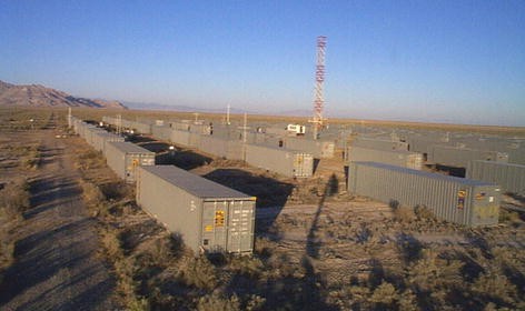
Containers and measurement towers of MUST field campaign
-
JU2003 (Joint Urban 2003, see [2]) is an atmospheric dispersion field study conducted in Oklahoma City and aimed at providing modeler with an actual in situ urban test case (see Figs. 5, 6).
Fig. 5 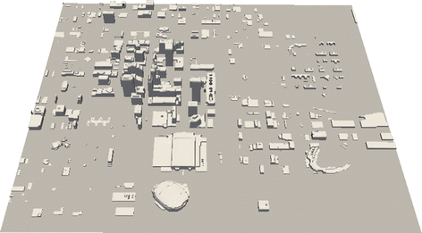
Large view of PMSS domain for Oklahoma City center, JU2003 test case (domain is 1.2 km × 1.2 km)
Fig. 6 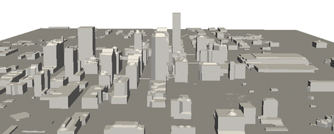
Close view looking eastward of PMSS domain for Oklahoma City, JU2003 test case


All the releases used here are continuous and the calculations are considered steady state, except for the JU2003 test case.
5.2 Experimental validation of PMSS
5.2.1 EMU
The current test uses only one of the EMU scenarios: a single L-shaped building with emissions located in the hook of the L. The atmosphere is neutral and the emission is continuous. Concentrations downwind of the building were compared to measurements at multiple sensors located in vertical planes downwind at x/H = 0.5, 1, 2, 5 and 10, where H is the building height. In each plane, between 48 and 80 measurements were available. For this test case, both DD and TFP/PP were used. The domain was divided evenly into 4 tiles, without any particular care to try to avoid splitting specific locations (see Fig. 7).

Top view of ground concentration contours 10 min after the release with the domain divided in four tiles (EMU test case)
Figure 8 displays a scatter plot of predicted VS measured concentrations. Results are satisfying as 54% of predicted concentrations are within a factor of 2, thus satisfying the acceptance criteria for urban dispersion model evaluation [14].

Scatter plot of predicted concentrations versus measured ones (kg/m3) for EMU test case (continuous line is perfect match, dashed lines are factor of 2)
5.2.2 MUST
The Mock Urban Setting Test (MUST) field experiment consisted in around 40 releases of tracer gas in an array of 120 obstacles on a flat ground. The obstacles were containers of dimensions 12.2 × 2.42 × 2.54 m. Release location changed between trials but remained in the vicinity of the first three rows of containers. Monitoring arrays were located roughly 25, 60, 95 and 120 m downwind of the release point. The 15 min trial of September 20, 2001 was selected due to the measurement quality. It is a continuous release. Both DD and TFP/PP were used on an evenly split domain (see Fig. 9).

Top view of ground concentration contours at 3:03 am (20/09/2001) with the domain divided in four tiles (MUST test case, domain size is 200 × 200 m)
The maximum observed and predict 15 mn-averaged concentrations on each array are compared. Half of predicted concentrations are within a factor of 2, and all of them are within a factor of 3. All maxima are over-predicted. No scatter plot is presented because concentration points are not numerous enough.
5.2.3 JU2003
Joint Urban 2003 experiment consisted of around 10 intensive operation periods (IOP) where a passive scalar was released in downtown Oklahoma City during July 2003. IOPs are a mix of nighttime and daytime releases and continuous/instantaneous releases. The first continuous release of IOP2 is used. Its duration is 30 min and it is a daytime release. Predicted concentrations are compared to the 40 measured concentrations located near the release point. Measured concentrations are averaged on 15 min durations. So are predicted concentrations. Comparisons are performed during the two 15 min halves of the release, which leads to around 80 comparison points. Both DD and TFP/PP were used on an unevenly split domain. Samples of wind field and concentration field can be seen on Figs. 10 and 11.

Close view near release point of wind vectors at 1.5 m (height above ground) at 4:00 pm (02/08/2003) with the domain divided in four tiles (JU2003 test case)

Top view of ground concentration contours at 4:15 pm (02/08/2003) with the domain divided in four tiles (JU2003 test case, domain is 1 km × 1 km)
Figure 12 displays a scatter plot of concentrations. Results are satisfying: 68% of predicted concentrations are within a factor of 2, thus satisfying the acceptance criteria for urban dispersion model evaluation [14].

Scatter plot of predicted concentrations versus measured ones (in ppt) for JU2003 test case (continuous line is perfect match, dashed lines are factor of 2)
5.3 Performances of PMSS
Speed-up S is defined as the ratio of the time T1 to perform the calculation with a single core divided by the time Tn obtained with n cores for the same calculation:
Ideal speed-up IS is obtained if using n cores leads to 1/nth of the time using a single core:
Performances have been tested against efficiency E defined as:
For instance, an efficiency of 50% means that if n cores are used, only 50% of the ideal speed-up is obtained. Since the speedup is limited, for instance by Amdahl’s law [17], then, and because IS = n, efficiency tends toward 0 as n tends to infinity.
Cluster used to evaluate performances consists of nodes of 4 dual-core processors Intel Itanium 2, clocked at 1.6 GHz.
5.3.1 Parallel-SWIFT performances
Parallel-SWIFT performances have been tested on:
-
MUST using TFP: 40 meteorological time frames have been submitted to the model, and tested using from 1 to 61 cores;
-
JU2003 using DD: the horizontal grid has 251 × 251 points. It has been tested using domain decomposition with up to 256 cores. When decomposing the domain using 256 cores, each individual tile has a horizontal grid of 16 × 16 points at the most.
Figure 13 displays the efficiency of Parallel-SWIFT on these two test cases. TFP for MUST is very good (efficiency above 80%) up to roughly 40 cores where it drops since no additional time frames can be computed in parallel. DD for JU2003 is less effective with an efficiency of 40–50%, related to the fact the domain is not split evenly. It drops when the size of tiles goes below 50 × 50 points. 50 × 50 points is considered a very small mesh size for a SWIFT calculation: typical meshes are within [100; 1000] points in each horizontal direction. DD limited performances are still acceptable since it is aimed primerly at weak scaling, i.e. calculation of very large domains too large to fit in the memory of a single processor.

Efficiency of parallel algorithms (TFP or DD) used in Parallel-SWIFT
5.3.2 Parallel-SPRAY performances
Parallel-SPRAY performances have been evaluated against JU2003 test case using 1.8 millions particles on up to 500 cores. Two different tests have been set up:
-
No domain decomposition (DD off): PP only is evaluated.
-
Domain is divided unevenly into 4 tiles: both PP and load balancing are used.
Figure 14 displays the efficiency of Parallel-SPRAY on these two test cases. Pure PP designed for strong scaling is very efficient: efficiency remains above 80% up to 40 cores (around 45,000 particles per core). Then, it hits 60% when reaching 100 cores (18,000 particles per core): the number of available particles limits the efficiency. The number of particles handled per each core must remain above what is considered small for a LPDM, around 100,000 particles.

Efficiency of parallel algorithms (PP and load balancing) used in Parallel-SPRAY
When the domain is subdivided, efficiency is less and around 60%, due to the cost of load balancing. Efficiency drops also earlier, at around 20 cores, compared to 40 cores in the case of the non-split domain: since the domain is split in four, each core tends to have 1/4 of particles available if the domain is not. Hence, the number of particles by core is going down to 100,000 particles sooner.
6 Conclusion and future work
MSS model is a fast transport and dispersion Röckle-type model for urban setup. Typical dense city calculations for a domain of roughly 1 km dimension at a resolution of 3 m, and 1 h simulation using 400,000 particles, take around 30 min on a 2015 laptop using a single Intel Core i5 core at 2.6 GHz (model 4288U). This is a moderate computational time to obtain the 3D detailed urban wind flow and atmospheric dispersion pattern of possibly noxious gases or fine particles. Expressed as an operational result like the hazardous zones for the population and the first responders, this can be useful information for rescue parties and local authorities.
However, a large number of Lagrangian particles or a long lasting or far reaching dispersion event or a large simulation domain (covering all or part of a city) may not be handled on a single core of a computer. Thus, parallelization is needed in both regards of the computational resources and physical models. In this respect, the MSS model has been parallelized using MPI technology to:
-
Increase the operational usage of the model by reducing the computational time (strong scaling through TFP and PP);
-
Get the ability to cope with arbitrary large simulation domains at high resolution using domain decomposition (weak scaling through DD).
MPI library makes it possible to use MSS both on multicore laptops and high performance computing clusters.
Parallel-MSS (PMSS) has undergone preliminary model validation on wind tunnel experiments (EMU), field experiment (MUST) and full-scale experiment in Oklahoma City (JU2003). Results are very encouraging: PMSS gave satisfactory dispersion results with more than 50% of predicted concentration within a factor of two of measurements. This is excellent considering [14] acceptance criterion in an urban environment which is FAC2 greater than 0.3. Regarding parallel performances for strong scaling, the efficiency of PMSS calculations has been tested up to a few hundred of cores. Strong scaling allows for an efficiency of up to 80%. A 30 min calculation can hence be reduced down to around 9 min using 4 cores, or 5 min using 8 cores.
Weak scaling has not been evaluated in this article. Still, calculations on very large domain of several tenths of kilometers at high resolution (3 m) are being done. These calculations may be performed to model the pollution due to traffic or accidental airborne hazards over a whole city, making use of huge and highly resolved domains setups on a supercomputer with up to 30,000 computing cores. Performances are yet to be evaluated to demonstrate PMSS ability to perform rapid simulations with a few meters horizontal resolution on an entire big city, a fact that would offer the perspective to operate real-time flow and dispersion even in the course of an emergency implying hazardous releases.
References
Allwine KJ, Clawson KL, Flaherty JE, Heiser JH, Hosker RP, Leach MJ, Stockham LW (2007) Urban dispersion program: urban measurements applied to emergency response. In: Seventh symposium on the urban environment, American meteorological society, vol 5, San Diego (CA), USA, September 2007
Allwine KJ, Leach MJ, Stockham LW, Shinn JS, Hosker RP, BowersJF, Pace JC (2004) Overview of joint urban 2003: an atmospheric dispersion study in Oklahoma City. In: Preprints of the symposium on planning, nowcasting and forecasting in the urban zone, American meteorological society, CD-ROM J, vol 7, Seattle (WA), USA, January 2004
Allwine KJ, Shinn JH, Streit GE, Clawson KL, Brown M (2002) Overview of urban 2000: a multiscale field study of dispersion through an urban environment. Bull Am Meteorol Soc 83(4):521–536
Biltoft CA, Yee E, Jones CD (2002) Overview of the Mock Urban Setting Test (MUST). In: Proceedings of the fourth symposium on the urban environment, May 2002, 20–24
Boris J, Fulton JE Jr, Obenschain K, Patnaik G, Young T Jr (2004) CT-analyst: fast and accurate CBR emergency assessment. In: Defense and security. International society for optics and photonics, pp 1–13
Brook DR, Felton NV, Clem CM, Strickland DCH, Griffiths IH, Kingdon RD, Hall DJ, Hargrave JM (2003) Validation of the urban dispersion model (UDM). Int J Environ Pollut 20(1–6):11–21
Brown MJ, Williams M (1998) An urban canopy parameterization for mesoscale meteorological models. In: Proceedings of the AMS conference on second urban environment symposium, November 1998, 2–7
Camelli FE, Hanna SR, Lohner R (2004) Simulation of the MUST field experiment using the FEFLO-urban CFD model. In: Fifth symposium on the urban environment, American meteorological society, CD-ROM 13.12, Vancouver (BC), Canada
Carissimo B, Macdonald RW (2002) A porosity/drag approach for the modeling of flow and dispersion in the urban canopy. In: Air pollution modeling and its application XV, Springer International Publishing, pp 385–393
Danzig R, Sageman M, Leighton T, Hough L, Yuki H, Kotani R, Hosford ZM (2011) Aum Shinrikyo—insights into how terrorists develop biological and chemical weapons. Center for a New American Society, July 2011
Gowardhan AA, Pardyjak ER, Senocak I, Brown MJ (2011) A CFD-based wind solver for an urban fast response transport and dispersion model. Environ Fluid Mech 11:439–464
Gowardhan AA, Pardyjak ER, Senocak I, Brown MJ (2007) Investigation of Reynolds stresses in a 3D idealized urban area using large eddy simulation. In: Proceedings of the AMS seventh symposium on urban environment, San Diego (CA), USA, paper J12.2
Hall RC (1997) Evaluation of model uncertainty (EMU)—CFD modelling of near-field atmospheric dispersion. Project EMU final report to the European Commission (Data CD also available with report), vol 7, WS Atkins Doc No. WSA/AM5017
Hanna SR, Chang JC (2012) Acceptance criteria for urban dispersion model evaluation. Meteorol Atmos Phys 116:133–146
Hanna S, Chang J, Hearn J, Hicks B, Fox S, Whitmire M, Spicer T, Brown D, Sohn M, Yamada T (2016) Deposition following accidental releases of chlorine from railcars. In: Air pollution modeling and its application XXIV, Springer International Publishing, pp 377–383
Hanna S, White J, Trolier J, Vernot R, Brown M, Gowardhan A, Kaplan H, Alexander Y, Moussafir J, Wang Y, Williamson C (2011) Comparisons of JU2003 observations with four diagnostic urban wind flow and Lagrangian particle dispersion models. Atmos Environ 45(24):4073–4081
Hill MD, Marty MR (2008) Amdahl’s law in the multicore era
Holmes NS, Morawska L (2006) A review of dispersion modelling and its application to the dispersion of particles: an overview of different dispersion models available. Atmos Environ 40(30):5902–5928
Hosker RP Jr (1984) Flow and diffusion near obstacles. In: Randerson D (ed) Atmospheric science and power production, DOE/TIC-27601, US Department of Energy, Washington DC, Ch. 7, pp 241–326
Kaplan H, Dinar N (1996) A Lagrangian dispersion model for calculating concentration distribution within a built-up domain. Atmos Environ 30(24):4197–4207
Leitl B, Trini Castelli S, Baumann-Stanzer K, Reisin TG, Barmpas Ph, Balczo M, Andronopoulos S, Armand P, Jurcakova K, Milliez M (2014) Evaluation of air pollution models for their use in emergency response tools in built environments: the ‘Michelstadt’ Case study in COST ES1006 action. In: Air pollution modeling and its application XXIII, Springer International Publishing, pp 395–399
Macdonald RW (2000) Modelling the mean velocity profile in the urban canopy layer. Bound-Layer Meteorol 97(1):25–45
McHugh CA, Carruthers DJ, Edmunds HA (1997) ADMS-urban: an air quality management system for traffic, domestic and industrial pollution. Int J Environ Pollut 8:666–674
Moussafir J, Oldrini O, Tinarelli G, Sontowsky J, Dougherty C (2004) A new operational approach to deal with dispersion around obstacles: the MSS software suite. In: Nineth international conference on harmonization within atmospheric dispersion modeling for regulatory purposes
Moussafir J, Olry C, Tinarelli G, Oldrini O, Harris T (2008) SWIFT and MSS current development. In: Twelfth annual George Mason University transport and dispersion modeling workshop
Patnaik G, Boris JP, Grinstein FF, Iselin JP (2003) Large scale urban simulation with the MILES approach. In: Annual AIAA CFD conference, AIAA paper 2003-4104, Orlando (FL), USA
Röckle R (1990) Bestimmung der Strömungsverhältnisse im Bereich komplexer Bebauungsstrukturen. PhD dissertation, Darmstadt, Germany
Rodean HC (1996) Stochastic lagrangian models of turbulent diffusion. American meteorological society, vol 45, Boston, USA
Sarrat C, Lemonsu A, Masson V, Guedalia D (2006) Impact of urban heat island on regional atmospheric pollution. Atmos Environ 40(10):1743–1758
Schulman LL, Strimaitis DG, Scire JS (2000) Development and evaluation of the PRIME plume rise and building downwash model. J Air Waste Manag Assoc 50(3):378–390
Smith WS, Brown MJ (2002) A CFD-generated wind field library feasibility study: maximum wind direction interval. In: Fourth symposium on the urban environment, May 2002, pp 196–197
Soulhac L, Salizzoni P, Cierco FX, Perkins R (2011) The model SIRANE for atmospheric urban pollutant dispersion—part I: presentation of the model. Atmos Environ 45(39):7379–7395
Sykes RI, Parker SF, Henn DS, Cerasoli CP, Santos LP (2000) PC-SCIPUFF version 1.3 technical documentation. ARAP Report No. 725. Titan Corporation, ARAP Group
Thomson DJ (1987) Criteria for the selection of stochastic models of particle trajectories in turbulent flows. J Fluid Mech 180:529–556
Tinarelli G, Brusasca G, Oldrini O, Anfossi D, Trini Castelli S, Moussafir J (2007) Micro-SWIFT-SPRAY (MSS): a new modelling system for the simulation of dispersion at microscale—general description and validation. In: Air pollution modeling and its application XVII. Springer International Publishing, pp 449–458
Tinarelli G, Mortarini L, Trini Castelli S, Carlino G, Moussafir J, Olry C, Armand P, Anfossi D (2013) Review and validation of Micro-SPRAY, a lagrangian particle model of turbulent dispersion. In: Lagrangian modeling of the atmosphere, geophysical monograph, vol 200, American Geophysical Union (AGU), May 2013, pp 311–328
Yee E, Lien FS, Ji H (2010) A building-resolved wind field library for vancouver: facilitating CBRN emergency response for the 2010 winter olympic games. Defense Research and Development, DRDC-Suffield-TM-2010-088, Suffield (AB), Canada
Author information
Authors and Affiliations
Corresponding author
Rights and permissions
About this article

Cite this article
Oldrini, O., Armand, P., Duchenne, C. et al. Description and preliminary validation of the PMSS fast response parallel atmospheric flow and dispersion solver in complex built-up areas. Environ Fluid Mech 17, 997–1014 (2017). https://doi.org/10.1007/s10652-017-9532-1
Received:
Accepted:
Published:
Issue Date:
DOI: https://doi.org/10.1007/s10652-017-9532-1