Compact FE for unbounded attribute-weighted sums for logspace from SXDH

Abstract

This paper presents the first functional encryption $(\textsf{FE})$ scheme for the attribute-weighted sum functionality that supports the uniform model of computation. In such an FE scheme, encryption takes as input a pair of attributes (x, z) where x is public and z is private. A secret key corresponds to some weight function f, and decryption recovers the weighted sum f(x)z. In our scheme, both the public and private attributes can be of arbitrary polynomial lengths that are not fixed at system setup. The weight functions are modelled as $\text {Logspace Turing machines}$. Prior schemes could only support non-uniform Logspace. The proposed scheme is proven adaptively simulation secure under the well-studied symmetric external Diffie–Hellman assumption against an arbitrary polynomial number of secret key queries both before and after the challenge ciphertext. This is the best possible security notion that could be achieved for FE. On the technical side, our contributions lie in extending the techniques of Lin and Luo [EUROCRYPT 2020] devised for indistinguishability-based payload hiding attribute-based encryption for uniform Logspace access policies and the “three-slot reduction” technique for simulation-secure attribute-hiding FE for non-uniform Logspace devised by Datta and Pal [ASIACRYPT 2021] to the context of simulation-secure attribute-hiding FE for uniform Logspace.

1 Introduction

Functional encryption (FE), formally introduced by Boneh et al. [24] and O’Neill [69], redefines the classical encryption procedure with the motivation to overcome the limitation of the “all-or-nothing” paradigm of decryption. In a traditional encryption system, there is a single secret key such that a user given a ciphertext can either recover the whole message or learns nothing about it, depending on the availability of the secret key. FE in contrast provides fine grained access control over encrypted data by generating artistic secret keys according to the desired functions of the encrypted data to be disclosed. More specifically, in a public-key FE scheme for a function class $\mathcal {F}$, there is a setup authority which produces a master secret key and publishes a master public key. Using the master secret key, the setup authority can derive secret keys or functional decryption keys $\textsf{SK}_f$ associated with functions $f \in \mathcal {F}$. Anyone can encrypt messages $\textsf{msg}$ belonging to a specified message space $\textsf{msg}\in \mathbb {M}$ using the master public key to produce a ciphertext $\textsf{CT}$. The ciphertext $\textsf{CT}$ along with a secret key $\textsf{SK}_f$ recovers the function of the message $f(\textsf{msg})$ at the time of decryption, while unable to extract any other information about $\textsf{msg}$. More specifically, the security of FE requires collusion resistance meaning that any polynomial number of secret keys together cannot gather more information about an encrypted message except the union of what each of the secret keys can learn individually.

By this time, we have a plethora of exciting works on $\textsf {FE}$. These works can be broadly classified in two categories. The first line of works attempted to build $\textsf{FE}$ for general functionalities [12,13,14,15,16,17, 20, 23, 25,26,27,28, 34, 41,42,50, 52, 53, 55, 60, 74]. However, those constructions were either only secure against bounded collusion and/or extremely inefficient. With the motivation to overcome these limitations, a second line of work attempted to design efficient FE schemes supporting arbitrary collusion of users for practically relevant functionalities, e.g., linear/quadratic functions [1,2,3,4,5,6,7,8,9,10,11, 21, 29, 32, 33, 35, 36, 38, 40, 54, 56, 61, 63,64,65,66, 70,71,72, 76, 77]. In this work, we advance the state of the art along the latter research direction.

$\textsf {FE}$ for Attribute-Weighted Sum Recently, Abdalla et al. [8] and Datta and Pal [38] studied FE schemes for a new class of functionalities termed as “attribute-weighted sums” ($\textsf{AWS}$). This is a generalization of the inner product functional encryption (IPFE) [3, 11]. In such a scheme, an attribute pair (x, z) is encrypted using the master public key of the scheme, where x is a public attribute (e.g., demographic data) and z is a private attribute containing sensitive information (e.g., salary, medical condition, loans, college admission outcomes). A recipient having a secret key corresponding to a weight function f can learn the attribute-weighted sum f(x)z. The attribute-weighted sum functionality appears naturally in several real life applications. For instance, as discussed by Abdalla et al. [8] if we consider the weight function f as a Boolean predicate, then the attribute-weighted sum functionality f(x) would correspond to the average z over all users whose attribute x satisfies the predicate f. Important practical scenarios include average salaries of minority groups holding a particular job ($z =$ salary) and approval ratings of an election candidate amongst specific demographic groups in a particular state ($z =$ rating).

The works of [8, 38] considered a more general case of the notion where the domain and range of the weight functions are vectors, in particular, the attribute pair of public/private attribute vectors $(\varvec{x}, \varvec{z})$, which is encrypted to a ciphertext $\textsf{CT}$. A secret key $\textsf{SK}_f$ generated for a weight function f allows a recipient to learn $f(\varvec{x})^{\top } \varvec{z}$ from $\textsf{CT}$ without leaking any information about the private attribute $\varvec{z}$.

The FE schemes of [8, 38] support an expressive function class of arithmetic branching programs (ABPs) which captures non-uniform Logspace computations. Both schemes were built in asymmetric bilinear groups of prime order and are proven secure in the simulation-based security model, which is known to be the desirable security model for FE [24, 69], under the (bilateral) k-Linear (k-Lin)/(bilateral) Matrix Diffie–Hellman ($\textsf{MDDH}$) assumption. The FE scheme of [8] achieves semi-adaptive security, where the adversary is restricted to making secret key queries only after making the ciphertext queries, whereas the FE scheme of [38] achieves adaptive security, where the adversary is allowed to make secret key queries both before and after the ciphertext queries.

However, as mentioned above, ABP is a non-uniform computational model. As such, in both the FE schemes [8, 38], the length of the public and private attribute vectors must be fixed at system setup. This is clearly a bottleneck in several applications of this primitive especially when the computation is done over attributes whose lengths vary widely among ciphertexts and are not fixed at system setup. For instance, suppose a government hires an external audit service to perform a survey on average salary of employees working under different job categories in various companies to resolve salary discrepancy. The companies create salary databases (X, Z) where $X = (x_i)_i$ contains public attributes $x_i = (\text {job title}, \text {department}, \text {company name})$ and $Z = (z_i)_i$ includes private attribute $z_i = \text {salary}$. To facilitate this auditing process without revealing individual salaries (private attribute) to the auditor, the companies encrypt their own database (X, Z) using an FE scheme for AWS. The government provides the auditor a functional secret key $\textsf{SK}_f$ for a function f that takes input a public attribute X and outputs 1 for $x_i$’s for which the “job title” matches with a particular job, say manager. The auditor decrypts ciphertexts of the various companies using $\textsf{SK}_f$ and calculates the average salaries of employees working under that job category in those companies. Now, if the existing FE schemes for AWS [8, 38] supporting non-uniform computations are employed then to make the system sustainable the government would have to fix a probable size (an upper bound) of the number of employees in all the companies. Also, the size of all ciphertexts ever generated would scale with that upper bound even if the number of employees in some companies, at the time of encryption, are much smaller than that upper bound. This motivates us to consider the following problem.

Open problem Can we construct an $\textsf{FE}$ scheme for $\textsf{AWS}$in some uniform computational model capable of handling public/private attributes of arbitrary length?

Our results This work resolves the above open problem. For the first time in the literature, we formally define and construct an FE scheme for unbounded $\textsf{AWS}$ ($\textsf{UAWS}$) functionality where the setup only depends on the security parameter of the system and the weight functions are modeled as $\text {Turing machines}$. The proposed $\textsf{FE}$ scheme supports both public and private attributes of arbitrary lengths. In particular, the public parameters of the system are completely independent of the lengths of attribute pairs. Moreover, the ciphertext size is compact meaning that it does not grow with the number of occurrences of a specific attribute in the weight functions which are represented as $\text {Logspace Turing machines}$. As a special case, we also obtain a FE scheme for attribute-weighted sums where the weight functions are modelled as deterministic finite automata (DFA). The schemes are adaptively simulation secure against the release of an unbounded (polynomial) number of secret keys both before and after the challenge ciphertext. As noted in [24, 69], simulation security is the best possible and the most desirable model for FE. Moreover, simulation-based security also captures indistinguishability-based security but the converse does not hold in general.

Our FE for $\textsf{UAWS}$ is proven secure in the standard model based on the symmetric external Diffie–Hellman (SXDH) assumption in the asymmetric prime-order pairing groups. Our main result in the paper is summarized as follows.

Theorem 1

(Informal) Assuming the $\textsf{SXDH}$ assumption holds in asymmetric pairing groups of prime-order, there exists an adaptively simulation secure $\textsf{FE}$ scheme for the attribute weighted sum functionality with the weight functions modeled as $\text {Logspace Turing machines}$ such that the lengths of public and private attributes are unbounded and can be chosen at the time of encryption, the ciphertexts are compact with respect to the multiple occurrences of attributes in the weight functions.

Viewing $\textsf{IPFE}$ as a special case of $\textsf{FE}$ for $\textsf{AWS}$, we also obtain the first adaptively simulation secure $\textsf{IPFE}$ scheme for unbounded length vectors (UIPFE), i.e., the length of the vectors is not fixed in setup. Observe that all prior simulation secure $\textsf{IPFE}$ [8, 10, 38, 76] could only support bounded length vectors, i.e., the lengths must be fixed in the setup. On the other hand, the only known construction of UIPFE [71] is proven secure in the indistinguishability-based model.

The proposed FE construction is semi-generic and extends the frameworks of the works of Lin and Luo [62] and Datta and Pal [38]. Lin and Luo [62] develop an adaptively secure attribute-based encryption (ABE) scheme for Logspace Turing machines proven secure in the indistinguishability-based model. Although the input length of their ABE is unbounded, but an ABE is an “all-or-nothing” type primitive which fully discloses the message to a secret key generated for accepting policies. Further, the ABE of [62] is only payload hiding secure meaning that the ciphertexts themselves can leak sensitive information about the associated attributes. In contrast, our FE for UAWS provides more fine grained encryption methodologies where the ciphertexts reveal nothing about the private part of associated attributes but their weighted sums. Our FE construction depends on two building blocks, an arithmetic key garbling scheme (AKGS) for $\text {Logspace Turing machines}$ which is an information-theoretic tool and a function hiding (bounded) slotted $\textsf{IPFE}$ scheme which is a computational primitive. An important motivation of [62] is to achieve compact ciphertexts for ABEs. In other words, they get rid of the so-called one-use restriction from prior adaptively secure ABEs [19, 30, 31, 57,58,59, 67, 68, 75] by replacing the core information-theoretic step with the computational primitive of function hiding slotted IPFE. The FE of [38] is able to accomplish this property for non-uniform computations by developing a three-slot encryption technique. Specifically, three slots are utilized to simulate the label functions obtained from the underlying AKGS garbling for pre-ciphertext secret keys. Note that, the three-slot encryption technique is an extension of dual system encryption methodologies [57, 58, 73]. In this work, we extend their frameworks [38, 62] to avoid the one-use restriction in the case of FE for UAWS that computes weights via $\text {Logspace Turing machines}$. It is non-trivial to implement such three-slot techniques in the uniform model. The main reason behind this fact is that in case of ABPs [38] the garbling randomness can be sampled knowing the size of ABPs, and hence the garbling algorithm is possible to run while generating secret keys. However, in the case of $\textsf{AKGS}$ for $\text {Logspace Turing machines}$, the garbling randomness depends on the size of the $\text {Turing machine}$ as well as its input lengths. Consequently, it is not possible to execute the garbling in the key generation or encryption algorithms as the information about the garbling randomness is distributed between these two algorithms. We tackle this by developing a more advanced three-slot encryption technique with distributed randomness which enables us to carry out such a sophisticated procedure for $\text {Logspace Turing machines}$.

Our FE for UAWS is a one-slot scheme. This means one pair of public–private attribute can be processed in a single encryption. An unbounded-slot FE for UAWS [8] enables us to encrypt unbounded many such pairs in a single encryption. Abdalla et al. [8] devise a generic transformation for bootstrapping from one-slot to unbounded-slot scheme. However, this transformation only works if the underlying one-slot scheme is semi-adaptively secure [38]. Thus, if we restrict our scheme to semi-adaptive security then using such transformations [8, 38] our one-slot FE scheme can be bootstrapped to support unbounded slots.

Current vs. preliminary versions A preliminary version [39] of this work has appeared in Asiacrypt 2022. This paper includes a significant and considerable amount of technical contributions compared to the preliminary version [39]. The previous version contains only the constructions of our single key, single ciphertext secure one-slot FE scheme and the one-slot FE scheme for Logspace without providing any formal treatment to the security analysis of these protocols. The preliminary version presents a very high level idea about the security analysis. Therefore, most of our technical contributions are not formalized in that version. We emphasize that representing and formalizing a proper sequence of hybrid experiments for the security analysis are crucial for understanding the technical challenges and their solutions which we provide in the current version. Especially, we not only describe a proof sketch (for each security analysis) but also depict the hybrid experiment in several tables (see Sects. 5 and 6) that clearly gives a concrete idea about the steps to prove the adaptive simulation security of our schemes. For example, the three-slot reduction mechanism devised in this paper for handling the pre-ciphertext keys of the one-slot FE scheme for $\text {Logspace Turing machines}$ are described in Tables 14, 15 and 16. Moreover, in Sect. 7 of the current version, we build a simpler FE scheme for attribute-weighted sums for deterministic finite automata or DFA. Note that, weight functions realized by DFA captures many real-life applications involving computation on unbounded data (or attributes) such as network logging, tax returns and virus scanners. Hence, our FE for DFA becomes more effective compared to the FE for $\text {Logspace Turing machines}$ for such potential applications.

Organization We discuss a detailed technical overview of our results in Sect. 2. We provide useful notations, related definitions, and complexity assumptions in Sect. 3. We give a description of AKGS construction for evaluating Turing machines via a sequence of matrix multiplications in Sect. 4. Our construction of a single key and single ciphertext secure $\textsf{FE}$ scheme for $\textsf{UAWS}$ can be found in Sect. 5. We provide the complete security analysis of the scheme in Sect. 5.2. Next, we build our full fledge 1-slot $\textsf{FE}$ scheme for $\textsf{UAWS}$ and prove its security in Sect. 6. We present our FE scheme for attribute-weighted sums for DFA in Sect. 7.

2 Technical overview

We now present an overview of our techniques for achieving an $\textsf{FE}$ scheme for $\textsf{AWS}$ functionality which supports the uniform model of computations. We consider prime-order bilinear pairing groups $(\mathbb {G}_1, \mathbb {G}_2, \mathbb {G}_{T }, g_1, g_2, e)$ with a generator $g_{T } = e(g_1, g_2)$ of $\mathbb {G}_{T }$ and denote $[\![a]\!]_i$ by an element $g_i^a \in \mathbb {G}_i$ for $i \in \{1, 2, T \}$. For any vector $\varvec{z}$, the k-th entry is denoted by $\varvec{z}[k]$ and [n] denotes the set $\{1, \ldots , n\}$.

The unbounded AWS functionality In this work, we consider an unbounded $\textsf{FE}$ scheme for the $\textsf{AWS}$ functionality for $\text {Logspace Turing machines}$ (or the class of $\textsf {L}$), in shorthand it is written as $\textsf{UAWS}^{\textsf {L}}$. More specifically, the setup only takes as input the security parameter of the system and is independent of any other parameter, e.g., the lengths of the public and private attributes. $\textsf{UAWS}^{\textsf {L}}$ generates secret keys $\textsf{SK}_{(\varvec{M}, \mathcal {I}_{\varvec{M}})}$ for a tuple of $\text {Turing machines}$ denoted by $\varvec{M} = \{M_k\}_{k \in \mathcal {I}_{\varvec{M}}}$ such that the index set $\mathcal {I}_{\varvec{M}}$ contains any arbitrary number of $\text {Turing machines}$ $M_k \in \textsf {L}$. The ciphertexts are computed for a pair of public–private attributes $(\varvec{x}, \varvec{z})$ whose lengths are arbitrary and are decided at the time of encryption. Precisely, the public attribute $\varvec{x}$ of length N comes with a polynomial time bound $T= \textsf{poly}(N)$ and a logarithmic space bound $S$, and the private attribute $\varvec{z}$ is an integer vector of length n. At the time of decryption, if $\mathcal {I}_{\varvec{M}}\subseteq [n]$ then it reveals an integer value $\sum _{k \in \mathcal {I}_{\varvec{M}}} M_k(\varvec{x})\varvec{z}[k]$. Since $M_k(\varvec{x})$ is binary, we observe that the summation selects and adds the entries of $\varvec{z}$ for which the corresponding $\text {Turing machine}$ accepts the public attribute $\varvec{x}$. On the other hand, if $\mathcal {I}_{\varvec{M}}]$ is not contained in [n] then the decryption cannot recover a meaningful information. An appealing feature of the functionality is that the secret key $\textsf{SK}_{(\varvec{M}, \mathcal {I}_{\varvec{M}})}$ can decrypt ciphertexts of unbounded length attributes in unbounded time/(logarithmic) space bounds. In contrast, existing $\textsf{FE}$ for $\textsf{AWS}$s [8, 38] are designed to handle non-uniform computations that can only handle attributes of bounded lengths and the public parameters grows linearly with the lengths. Next, we describe the formulation of $\text {Turing machines}$ in $\textsf {L}$ considered in $\textsf{UAWS}^{\textsf {L}}$.

Turing machines formulation We introduce the notations for Logspace Turing machines ($\textsf{TM}$) over binary alphabets. A $\text {Turing machine}$ $M = (Q, \varvec{y}_{\textsf{acc}}, \delta )$ consists of Q states with the initial state being 1 and a characteristic vector $\varvec{y}_{\textsf{acc}} \in \{0, 1\}^Q$ of accepting states and a transition function $\delta$. When an input $(\varvec{x}, N, T, S)$ with length N and time, space bounds $T, S$ is provided, the computation of $M|_{N, T, S}(\varvec{x})$ is performed in $T$ steps passing through configurations $(\varvec{x}, (i, j, \varvec{W}, q))$ where $i \in [N]$ is the input tape pointer, $j \in [S]$ is the work tape pointer, $\varvec{W} \in \{0, 1\}^{S}$ the content of work tape, and $q \in [Q]$ the state under consideration. The initial internal configuration is $(1, 1, {{\textbf {0}}}_{S}, 1)$ and the transition function $\delta$ determines whether, on input $\varvec{x}$, it is possible to move from one internal configuration $(i, j, \varvec{W}, q)$ to the next $((i', j', \varvec{W}', q'))$, namely if $\delta (q, \varvec{x}[i], \varvec{W}[j]) = (q', w', \mathrm {\varDelta } i, \mathrm {\varDelta } j)$. In other words, the transition function $\delta$ on input state q, an input bit $\varvec{x}[i]$ and an work tape bit $\varvec{W}[j]$, outputs the next state $q'$, the new bit $w'$ overwriting $w = \varvec{W}[j]$ by $w' = \varvec{W}'[j]$ (keeping $\varvec{W}[j''] = \varvec{W}'[j'']$ for all $j \ne j''$), and the directions $\mathrm {\varDelta } i, \mathrm {\varDelta } j\in \{0, \pm 1\}$ to move the input and work tape pointers.

Our construction of adaptively simulation secure $\textsf{UAWS}^{\textsf {L}}$ depends on two building blocks: $\textsf{AKGS}$ for $\text {Logspace Turing machines}$, an information-theoretic tool and slotted $\textsf{IPFE}$, a computationally secure tool. We only need a bounded slotted $\textsf{IPFE}$, meaning that the length of vectors of the slotted $\textsf{IPFE}$ is fixed in the setup, and we only require the primitive to satisfy adaptive indistinguishability based security. Hence, our work shows how to (semi-)generically bootstrap a bounded $\textsf{IPFE}$ to an unbounded $\textsf{FE}$ scheme beyond the inner product functionality. Before going to describe the $\textsf{UAWS}^{\textsf {L}}$, we briefly discuss these two building blocks.

AKGS for Logspace Turing machines In [62], the authors present an ABE scheme for $\text {Logspace Turing machines}$ by constructing an efficient $\textsf{AKGS}$ for sequence of matrix multiplications over $\mathbb {Z}_p$. Thus, their core idea was to represent a $\text {Turing machine}$ computation through a sequence of matrix multiplications. An internal configuration $(i, j, \varvec{W}, q)$ is represented as a basis vector $\varvec{e}_{(i, j, \varvec{W}, q)}$ of dimension $NS2^{S}Q$ with a single 1 at the position $(i, j, \varvec{W}, q)$. We define a transition matrix given by

such that $\varvec{e}_{(i, j, \varvec{W}, q)}^{\top }{{\textbf {M}}}(\varvec{x})$ $=$ $\varvec{e}_{(i', j', \varvec{W}', q')}^{\top }$. This holds because the $((i, j, \varvec{W}, q), (i', j', \varvec{W}', q'))$-th entry of ${{\textbf {M}}}(\varvec{x})$ is 1 if and only if there is a valid transition from $(q, \varvec{x}[i], \varvec{W}[j])$ to $(q', \varvec{W}'[j], i'-i, j'-j)$. Therefore, one can write the $\text {Turing machine}$ computation by right multiplying the matrix ${{\textbf {M}}}(\varvec{x})$ for $T$ times with the initial configuration $\varvec{e}_{(1, 1, \varvec{0}_{S}, 1)}^{\top }$ to reach of one of the final configurations ${{\textbf {1}}}_{[N]\times [S]\times \{0, 1\}^{S}} \otimes \varvec{y}_{\textsf{acc}}$. In other words, the function $M|_{N, T, S}(\varvec{x})$ is written as

$$\begin{aligned} M|_{N, T, S}(\varvec{x}) = \varvec{e}_{(1, 1, \varvec{0}_{S}, 1)}^{\top } ({{\textbf {M}}}_{N, S}(\varvec{x}))^{T} (\varvec{1}_{[N]\times [S] \times \{0, 1\}^{S}}\otimes \varvec{y}_{\textsf{acc}}) \end{aligned}$$

(1)

Thus, [62] constructs an $\textsf{AKGS}$ for the sequence of matrix multiplications as in Eq. (1). Their $\textsf{AKGS}$ is inspired from the randomized encoding scheme of [18] and homomorphic evaluation procedure of [22]. Given the function $M|_{N, T, S}$ over $\mathbb {Z}_p$ and two secrets $z, \beta$, the garbling procedure computes the label functions

$$\begin{aligned} \begin{array}{r l} L_{\textsf{init}}(\varvec{x}) &{} = \beta + \varvec{e}_{(1, 1, \varvec{0}_{S}, 1)}^{\top }\varvec{r}_0,\\ \text {for } t \in [T]:~~ (L_{t, \theta })_{\theta }(\varvec{x}) &{} = -\varvec{r}_{t-1} + {{\textbf {M}}}_{N, S}(\varvec{x})\varvec{r}_t,\\ (L_{T+1, \theta })_{\theta }(z) &{} = -\varvec{r}_{T} + z \varvec{1}_{[N]\times [S] \times \{0, 1\}^{S}} \otimes \varvec{y}_{\textsf{acc}}. \end{array} \end{aligned}$$

and outputs the coefficients of these label functions $\ell _{\textsf{init}}, \varvec{\ell }_t = (\varvec{\ell }_{t, \theta })_{\theta }$ where $\theta = (i, j, \varvec{W}, q)$ and $\varvec{r}_t \leftarrow \mathbb {Z}_p^{[N] \times [S] \times \{0, 1\}^{S} \times [Q]}$. To compute the functional value for an input $\varvec{x}$, the evaluation procedure adds $\ell _{\textsf{init}}$ with a telescoping sum $\varvec{e}_{(1, 1, \varvec{0}_{S}, 1)}^{\top }\cdot \sum _{t= 1}^{T} ({{\textbf {M}}}_{N, S}(\varvec{x}))^{t-1} \varvec{\ell }_t$ and outputs $zM|_{N, T, S}(\varvec{x}) + \beta$. More precisely, it uses the fact that

$$\begin{aligned} \begin{array}{l} \varvec{e}_{i_{t+1}, j_{t+1}, \varvec{W}_{t+1}, q_{t+1}}^{\top } \varvec{r}_{t+1} \\ = \varvec{e}_{i_{t}, j_{t}, \varvec{W}_{t}, q_{t}}^{\top } \varvec{r}_{t} + \varvec{e}_{i_{t}, j_{t}, \varvec{W}_{t}, q_{t}}^{\top } (\underbrace{-\varvec{r}_t + {{\textbf {M}}}(\varvec{x})\varvec{r}_{t+1}}_{\varvec{\ell }_{t+1}})\end{array} \end{aligned}$$

A crucial and essential property that the $\textsf{AKGS}$ have is the linearity of evaluation procedure, meaning that the procedure is linear in the label function values $\ell$s and, hence can be performed even if the $\ell$s are available in the exponent of a group. Lin and Luo identify two important security notions of $\textsf{AKGS}$, jointly called piecewise security. Firstly, $\ell _{\textsf{init}}$ can be reversely sampled given a functional value and all other label values, which is known as the reverse sampleability. Secondly, $\ell _{t}$ is random with respect to the subsequent label functions $L_{t', \theta }$ for all $t' > t$ and z, which is called the marginal randomness.

Function hiding slotted IPFE A normal $\textsf{IPFE}$ computes inner product between two vectors $\varvec{v}$ and $\varvec{u}$ using a secret key $\textsf{IPFE}.\textsf{SK}_{\varvec{v}}$ and a ciphertext $\textsf{IPFE}.\textsf{CT}_{\varvec{u}}$. The $\textsf{IPFE}$ is said to satisfy indistinguishability-based security if an adversary having received many functional secret keys $\{\textsf{IPFE}.\textsf{SK}_{\varvec{v}}\}$ remains incapable to extract any information about the message vector $\varvec{u}$ except the inner products $\{{\varvec{v}} \cdot {\varvec{u}}\}$. It is easy to observe that if encryption is done publicly then no security can be ensured about $\varvec{v}$ from the secret key $\textsf{IPFE}.\textsf{SK}_{\varvec{v}}$ [36] due to the linear functionality. However, if the encryption algorithm is private then $\textsf{IPFE}.\textsf{SK}_{\varvec{v}}$ can be produced in a fashion to hide sensitive information about $\varvec{v}$. This is termed as function hiding security notion for private key $\textsf{IPFE}$. Slotted $\textsf{IPFE}$ [64] is a hybrid of public and private $\textsf{IPFE}$ where vectors are divided into public and private slots, and function hiding is only guaranteed for the entries in the private slots. Further, Slotted $\textsf{IPFE}$s of [62, 64] generate secret keys and ciphertexts even when the vectors are given in the exponent of source groups whereas decryption recovers the inner product in the target group.

2.1 From all-or-nothing to functional encryption

We are all set to describe our approach to extend the framework of [62] from all-or-nothing to functional encryption for the uniform model of computations. In a previous work of Datta and Pal [38], an adaptively secure FE for $\textsf{AWS}$ functionality was built for a non-uniform model of computation, ABPs to be precise. Their idea was to garble a function $f_k(\varvec{x})\varvec{z}[k] + \beta _k$ during key generation (keeping $\varvec{z}[k]$ and $\varvec{x}$ as variables) and compute IPFE secret keys to encode the m labels, and a ciphertext associated to a tuple $(\varvec{x}, \varvec{z})$ consists of a collection of $\textsf{IPFE}$ ciphertexts which encode the attributes:

Therefore, using the inner product functionality, decryption computes the actual label values with $\varvec{x}, \varvec{z}[k]$ as inputs and recovers $f_k(\varvec{x})\varvec{z}[k] + \beta _k$ for each k, and hence finally $\sum _{k} f_k(\varvec{x})\varvec{z}[k]$. However, this approach fails to build $\textsf{UAWS}^{\textsf {L}}$ because we can not execute the $\textsf{AKGS}$ garbling for the function $M_k|_{N, T, S}(\varvec{x})\varvec{z}[k]+\beta _k$ at the time of generating keys. More specifically, the garbling randomness depends on parameters $N, T, S, n$ that are unknown to the key generator. Note that, in contrast to the $\textsf {ABE}$ of [62] where $\varvec{z}$ can be viewed as a payload (hence $n=1$), the $\textsf{UAWS}$ functionality has an additional parameter n (length of $\varvec{z}$) the value of which is chosen at the time of encryption. Moreover, the compactness of $\textsf{UAWS}^{\textsf {L}}$ necessitates the secret key size $|\textsf{SK}_{(\varvec{M}, \mathcal {I}_{\varvec{M}})}| = O(|\mathcal {I}_{\varvec{M}}|Q)$ to be linear in the number of states Q and the ciphertext size $|\textsf{CT}_{(\varvec{x}, T, S)}| = O(n TN S2^{S})$ be linear in $TN S2^{S}$.

The obstacle is circumvented by the randomness distribution technique used in [62]. Instead of computing the $\textsf{AKGS}$ garblings in key generation or encryption phase, the label values are produced by a joint effort of both the secret key and ciphertext. To do so, the garbling is executed under the hood of $\textsf{IPFE}$ using pseudorandomness, instead of true randomness. That is, some part of the garbling randomness is sampled in key generation whereas the rest is sampled in encryption. More specifically, every true random value $\varvec{r}_t[(i, j, \varvec{W}, q)]$ is written as a product $\varvec{r}_{\varvec{x}}[(t,i,j,\varvec{W})]\varvec{r}_{k, f}[q]$ where $\varvec{r}_{\varvec{x}}[(t,i,j,\varvec{W})]$ is used in the ciphertext and $\varvec{r}_{k, f}[q]$ is utilized to encode the transition blocks of $M_k$ in the secret key. To enable this, the transition matrix associated to $M_k$ is represented as follows:

$\begin{array}{ l} {{\textbf {M}}}(\varvec{x})[(i, j, \varvec{W}, q),(i', j', \varvec{W}', q')] \\ = \delta ^{(?)}((i, j, \varvec{W}, q), (i', j', \varvec{W}', q'))\times ~{{\textbf {M}}}_{\varvec{x}[i], \varvec{W}[j], \varvec{W}'[j], i'-i, j'-j}[q, q'] \end{array}$

where $\delta ^{(?)}((i, j, \varvec{W}, q), (i', j', \varvec{W}', q'))$ is 1 if there is a valid transition from the configuration $(i, j, \varvec{W}, q)$ to $(i', j', \varvec{W}', q')$, otherwise 0. Therefore, every block of ${{\textbf {M}}}(\varvec{x})[(i, j, \varvec{W}, q),(i', j', \varvec{W}', q')]$ is either a $Q \times Q$ zero matrix or a transition block that belongs to a small set

$$\begin{aligned} \mathcal {T} = \{{{\textbf {M}}}_{\tau } | ~~\tau = (x, w, w', \mathrm {\varDelta } i, \mathrm {\varDelta } j) \in \{0, 1\}^3 \times \{0, \pm 1\}^2 \} \end{aligned}$$

The $(i, j, \varvec{W}, q)$-th block row ${{\textbf {M}}}_{\tau } = {{\textbf {M}}}_{x, w, w', \mathrm {\varDelta } i, \mathrm {\varDelta } j}$ appears at ${{\textbf {M}}}_{N, S}(\varvec{x})[(i, j, \varvec{W}, \textvisiblespace ), (i', j', \varvec{W}', \textvisiblespace )]$ if $x = \varvec{x}[i], w = \varvec{W}[j], \mathrm {\varDelta } i= i' - i, \mathrm {\varDelta } j= j' - j$, and $\varvec{W}'$ is $\varvec{W}$ with j-th entry changed to $w'$. Thus, every label $\varvec{\ell }_{k, t}[\mathfrak {i}, q]$ with $\mathfrak {i} = (i, j, \varvec{W})$ can be decomposed as inner product ${\varvec{v}_{k, q}} \cdot {\varvec{u}_{k, t, i, j, \varvec{W}}}$. More precisely,

so that one can set the vectors

$$\begin{aligned} \begin{array}{r l c c c c c c} \varvec{v}_{k, q} &{} = (&{} -\varvec{r}_{k, f}[q],&{} 0,&{} ({{\textbf {M}}}_{k, \tau }\varvec{r}_{k, f})[q] &{}~ \Vert ~&{} \varvec{0}&{}), \\ \varvec{u}_{t, \mathfrak {i}} &{} = (&{} \varvec{r}_{\varvec{x}}[t-1, \mathfrak {i}],&{} 0,&{} c_{\tau }(\varvec{x}; \varvec{r}_{\varvec{x}})&{} ~ \Vert ~&{} \varvec{0}&{}) \end{array} \end{aligned}$$

where $c_{\tau }(\varvec{x}; \varvec{r}_{\varvec{x}})$ (a shorthand of the notation $c_\tau (\varvec{x},t,i,j,\varvec{W};\varvec{r}_{\varvec{x}})$ [62]) is given by

$$\begin{aligned} c_{\tau }(\varvec{x}; \varvec{r}_{\varvec{x}}) = {\left\{ \begin{array}{ll} \varvec{r}_{\varvec{x}}[t,\mathfrak {i}'], &{}~~ \text {if } x = \varvec{x}[i], w = \varvec{W}[j];\\ 0, &{}~~\text {otherwise}. \end{array}\right. } \end{aligned}$$

Similarly, the other labels can be decomposed: $\ell _{k, \textsf{init}} = (\varvec{r}_{k, f}[1], \beta _k, 0)\cdot (\varvec{r}_{\varvec{x}}[(0, 1, 1, \varvec{0}_{S})], 1, 0) = \beta _k + \varvec{e}_{(1, 1, \varvec{0}_{S}, 1)}^{\top }\varvec{r}_0$ and $\varvec{\ell }_{k, T+1}[(\mathfrak {i}, q)] = {\widetilde{\varvec{v}}_{k, q}} \cdot {\widetilde{\varvec{u}}_{k, T+1, i, j, \varvec{W}}} = -\varvec{r}_{T}[(\mathfrak {i}, q)] + \varvec{z}[k] \varvec{y}_{k, \textsf{acc}}[q]$ where

$$\begin{aligned} \begin{array}{r l c c c c c} \widetilde{\varvec{v}}_{k, q} &{} = (&{} -\varvec{r}_{k, f}[q],&{} \varvec{y}_{k, \textsf{acc}}[q]&{}~ \Vert ~&{} \varvec{0}&{}), \\ \widetilde{\varvec{u}}_{T+1, \mathfrak {i}} &{} = (&{} \varvec{r}_{\varvec{x}}[T, \mathfrak {i}],&{} \varvec{z}[k]&{} ~ \Vert ~&{} \varvec{0}&{}) \end{array} \end{aligned}$$

A first attempt Armed with this, we now present the first candidate $\textsf{UAWS}^{\textsf {L}}$ construction in the secret key setting which supports a single key. We consider two independent master keys $\textsf {imsk}$ and $\widetilde{\textsf {imsk}}$ of $\textsf{IPFE}$. For simplicity, we assume the length of the private attribute $\varvec{z}$ is the same as the number of $\text {Turing machines}$ present in $\varvec{M} = (M_k)_{k \in \mathcal {I}_{\varvec{M}}}$, i.e., $n = |\mathcal {I}_{\varvec{M}}|$. We also assume that each Turing machine in the secret key shares the same set of states.

Observe that the inner products between the ciphertext and secret key vectors yield the label values $[\![\ell _{k, \textsf{init}}]\!]_{T }, [\![\varvec{\ell }_{k, t}]\!]_{T } = [\![(\varvec{\ell }_{k, t, \theta })_{\theta }]\!]_{T }$ for $\theta = (i, j, \varvec{W}, q)$. Now, the evaluation procedure of $\textsf{AKGS}$ is applied to obtain the partial values $[\![\varvec{z}[k]M_k|_{N, T, S}(\varvec{x}) + \beta _k]\!]_{T }$. Combining all this values gives the required attribute weighted sum $\sum _{k}M_k|_{N, T, S}(\varvec{x})\varvec{z}[k]$ Since $\sum _k \beta _k = 0$.

However, this scheme is not fully unbounded, in particular, the setup needs to know the length of the private attribute. To realise this, let us try to prove the security of the scheme. The main idea of the proof would be to make all the label values $(\varvec{\ell }_{k, t, \theta })_{\theta }$ truly random and simulated except the initial labels $\ell _{k, \textsf{init}}$ so that one can reversely sample $\ell _{k, \textsf{init}}$ hardcoded with a desired functional value. Suppose, for instance, the single secret key is queried before the challenge ciphertext. In this case, the honest label values are first hardwired in the ciphertext vectors and then the labels are transformed into their simulated version. This is because the ciphertext vectors are computed after the secret key. So, the first step is to hardwire the initial label values $\ell _{k, \textsf{init}}$ into the ciphertext vector $\varvec{u}_{\textsf{init}}$, which indicates that the length of $\varvec{u}_{\textsf{init}}$ must grow with respect to the number of $\ell _{k, \textsf{init}}$’s. The same situation arises while simulating the other label values through $\varvec{u}_{t, \mathfrak {i}}$. In other words, we need to know the size of $\mathcal {I}_{\varvec{M}}$ or the length of $\varvec{z}$ in setup, which is against our desired functionality.

To tackle this, we increase the number of $\varvec{u}_{\textsf{init}}$ and $\varvec{u}_{t<T, \mathfrak {i}}$ in the above system. More specifically, each of these vectors are now computed for all $k \in [n]$, just like $\widetilde{\varvec{u}}_{k, T+1, \mathfrak {i}}$. Although this fixes the requirement of unboundedness of the system, there is another issue related to the security that must be solved. Note that, in the current structure, there is a possibility of mix-and-match attacks since, for example, $\widetilde{\varvec{u}}_{k_1, T+1, \mathfrak {i}}$ can be paired with $\widetilde{\varvec{v}}_{k_2, q}$ and this results in some unwanted attribute weighted sum of the form $\sum _{k \ne k_1, k_2}M_k(\varvec{x})\varvec{z}[k] + M_{k_1}(\varvec{x})\varvec{z}[k_2] + M_{k_2}(\varvec{x})\varvec{z}[k_1]$. We employ the index encoding technique used in previous works achieving unbounded ABE or $\textsf{IPFE}$ [68, 71] to overcome the attack. In particular, we add two extra dimensions $\rho _k(-k, 1)$ in the ciphertext and $\pi _k(1, k)$ in the secret key for encoding the index k in each of the vectors of the system. Observe that for each $\text {Turing machine}$ $M_k$ an independent randomness $\pi _k$ is sampled. It ensures that an adversary can only recover the desired attribute weighted sum and whenever vectors from different indices are paired only a garbage value is obtained.

Combining the ideas After combining the above ideas, we describe our $\textsf{UAWS}^{\textsf {L}}$ supporting a single key as follows.

Although the above construction satisfies our desired functionality, preserves the compactness of ciphertexts and resists the aforementioned attack, we face multiple challenges in adapting the proof ideas of previous works [38, 62, 71].

Security challenges and solutions Next, we discuss the challenges in proving the adaptive simulation security of the scheme. Firstly, the unbounded $\textsf{IPFE}$ scheme of Tomida and Takashima [71] is proved in the indistinguishability-based model whereas we aim to prove simulation security which is much more challenging. The work closer to ours is the FE for $\textsf{AWS}$ of Datta and Pal [38], but it only supports a non-uniform model of computation and the inner product functionality is bounded. Moreover, since the garbling randomness is distributed in the secret key and ciphertext vectors, we can not adapt their proof techniques [38, 71] in a straightforward manner. Although the ABE scheme of Lin and Luo [62] handles a uniform model of computation, they only consider all-or-nothing type encryptions and hence the adversary is allowed to query secret keys which always fail to decrypt the challenge ciphertext. In contrast, we construct a more advanced encryption mechanism which overcomes all the above constraints of prior works, i.e., our $\textsf{UAWS}^{\textsf {L}}$ is an adaptively simulation secure functional encryption scheme that supports unbounded inner product functionality with a uniform model of computations over the public attributes.

Our proof technique is inspired by that of [38, 62]. One of the core technical challenges is involved in the case where the secret key is queried before the challenge ciphertext. Thus, we focus more on “$\textsf {sk}$ queried before $\textsf {ct}$” in this overview. As noted above, in the security analysis of [62] the adversary $\mathcal {A}$ is not allowed to decrypt the challenge ciphertext and hence they completely randomize the ciphertext in the final game. However, since we are building a FE scheme any secret key queried by $\mathcal {A}$ should be able to decrypt the challenge ciphertext. For this, we use the pre-image sampleability technique from prior works [37, 38]. In particular, the reduction samples a dummy vector $\varvec{d} \in \mathbb {Z}_p^n$ satisfying $\sum _{k}M_k|_{N, T, S}(\varvec{x})\varvec{z}[k] = \sum _{k}M_k|_{N, T, S}(\varvec{x})\varvec{d}[k]$ where $\varvec{M} = (M_k)_k$ is a pre-challenge secret key. To plant the dummy vector into the ciphertext, we first need to make all label values $\{\ell _{k, t, \mathfrak {i}, q}\}$ truly random depending on the terms $\varvec{r}_{k, f}[q]\varvec{r}_{\varvec{x}}[t-1, \mathfrak {i}]$’s and then turn them into their simulated forms, and finally traverse in the reverse path to get back the original form of the ciphertext with $\varvec{d}$ taking place of the private attribute $\varvec{z}$. In order to make all these labels truly random, the honest label values are needed to be hardwired into the ciphertext vectors (since these are computed later) so that we can apply the DDH assumption in $\mathbb {G}_1$ to randomize the term $\varvec{r}_{k, f}[q]\varvec{r}_{\varvec{x}}[t-1, \mathfrak {i}]$ (hence the label values). However, this step is much more complicated than in [62] since there are two independent $\textsf{IPFE}$ systems in our construction and $\varvec{r}_{k, f}[q]$ appears in both $\varvec{v}_{k, q}$ and $\widetilde{\varvec{v}}_{k, q}$ (i.e., in both $\textsf{IPFE}$ systems). We design a two-level nested loop running over q and t for relocating $\varvec{r}_{k, f}[q]$ from $\varvec{v}$’s and $\widetilde{\varvec{v}}_{k, q}$ to $\varvec{u}$’s and $\widetilde{\varvec{u}}_{k, T+1, \mathfrak {i}}$. To this end, we note that the case of “$\textsf {sk}$ queried after $\textsf {ct}$” is simpler where we embed the reversely sampled initial label values into the secret key. Before going to discuss the hybrids, we first present the simulator of the ideal world.

Security analysis We use a three-step approach and each step consists of a group of hybrid sequence. At a very high level, we discuss the case of “$\textsf {sk}$ queried before $\textsf {ct}$”. In this overview, for simplicity, we assume that the challenger knows the length of $\varvec{z}$ while it generates the secret key.

First group of hybrids The reduction starts with the real scheme. In the first step, the label function $\ell _{k, \textsf{init}}$ is reversely sampled with the value $M_k[\varvec{x}]\varvec{z}[k] + \beta _k$ which is hardwired in $\varvec{u}_{k, \textsf{init}}$.

$\begin{aligned}&\begin{array}{r l c c c c c c c c} \varvec{v}_{k, \textsf{init}} &{} = (&{} \cdots , &{} \boxed {1},&{} \boxed {0},&{} 0 &{}~ \Vert ~&{} 0, &{} \varvec{0}&{}),\\ \varvec{v}_{k, q} &{} = (&{} \cdots , &{} -\varvec{r}_{k, f}[q],&{} 0,&{} ({{\textbf {M}}}_{k, \tau }\varvec{r}_{k, f})[q] &{}~ \Vert ~&{} \boxed {\varvec{s}_{k, f}[q]}, &{} \varvec{0}&{}),\\ \widetilde{\varvec{v}}_{k, q} &{} = (&{} \cdots , &{} -\varvec{r}_{k, f}[q],&{} \varvec{y}_{k, \textsf{acc}}[q]&{} &{}~ \Vert ~&{} 0, &{}\varvec{0}&{}) \end{array}\\&\begin{array}{r l c c c c c c c c} \varvec{u}_{k, \textsf{init}} &{} = (&{} \cdots , &{} \boxed {\ell _{k, \textsf{init}}},&{} \boxed {0},&{} 0, &{}~ \Vert ~&{} 0, &{} \varvec{0}&{}),\\ \varvec{u}_{k, t<T, \mathfrak {i}} &{} = (&{}\cdots , &{} \varvec{r}_{\varvec{x}}[t-1, \mathfrak {i}],&{} 0,&{} c_{\tau }(\varvec{x}; \varvec{r}_{\varvec{x}})&{} ~ \Vert ~&{} 0, &{} \varvec{0}&{}),\\ \widetilde{\varvec{u}}_{k, T+1, \mathfrak {i}} &{} = (&{} \cdots , &{} \varvec{r}_{\varvec{x}}[T, \mathfrak {i}],&{} \varvec{z}[k]&{} &{}~ \Vert ~&{} \boxed {\varvec{s}_{\varvec{x}}[T+1, \mathfrak {i}]}, &{}\varvec{0}&{}) \end{array} \end{aligned}$

where $\ell _{k, \textsf{init}} \leftarrow \textsf {RevSamp}((M_k, \varvec{x}, M_k[\varvec{x}]\varvec{z}[k] + \beta _k, \{\ell _{k, t, \mathfrak {i},q}\})$ and $\ell _{k, t, \mathfrak {i},q}$’s are computed honestly. Note that, the secret values $\{\beta _k\}$ are sampled depending on whether the queried key is eligible for decryption. More specifically, if $\mathcal {I}_{\varvec{M}}\subseteq [n]$, then $\beta _k$’s are sampled as in the original key generation algorithm, i.e., $\sum _k \beta _k = 0$. On the other hand, if $\text {max} \mathcal {I}_{\varvec{M}}> n$ then $\beta _k$’s are sampled uniformly at random, i.e., they do not necessarily be secret shares of zero. This can be done by the function hiding property of $\textsf{IPFE}$ which ensures that the distributions $\{ \{\textsf{IPFE}.\textsf{SK}_{\varvec{v}_k^{(\mathfrak {b})}}\}_{k \in [n+1, |\mathcal {I}_{\varvec{M}}|]} , \{\textsf{IPFE}.\textsf{CT}_{\varvec{u}_{k'}}\}_{ k' \in [n]} \}$ for $\mathfrak {b} \in \{0, 1\}$ are indistinguishable where

$\begin{array}{r l c c c c c c l} \varvec{v}_k^{(\mathfrak {b} )} &{}= (&{} \pi _k,&{} k\cdot \pi _k,&{} \varvec{0},&{} \beta _k + \mathfrak {b}\cdot r_k,&{} \varvec{0}&{}) &{}\text {~ for }k \in [n+1, |\mathcal {I}_{\varvec{M}}|], r_k \leftarrow \mathbb {Z}_p \\ \varvec{u}_{k'} &{} = (&{} -k' \cdot \rho _{k'},&{} \rho _{k'},&{} \varvec{0},&{} 1,&{} \varvec{0}&{})&{}\text {~ for }k' \in [n]\\ \end{array}$

Thus, the indistinguishability between the group of hybrids can be guaranteed by the piecewise security of $\textsf{AKGS}$ and the function hiding security of $\textsf{IPFE}$.

Second group of hybrids The second step is a loop. The purpose of the loop is to change all the honest label values $\ell _{k, t, \mathfrak {i}, q}$ to simulated ones that take the form $\ell _{k, t, \mathfrak {i}, q} = \varvec{s}_{\varvec{x}}[t, \mathfrak {i}]\varvec{s}_{k, f}[q]$ where $\varvec{s}_{\varvec{x}}[t, \mathfrak {i}]$ is hardwired in $\varvec{u}_{k, t, \mathfrak {i}}$ or $\widetilde{\varvec{u}}_{k, T+1, \mathfrak {i}}$ and $\varvec{s}_{k, f}[q]$ is hardwired in $\varvec{v}_{k,q}$ or $\widetilde{v}_{k, q}$.

The whole procedure is executed in via a two-level loop with outer loop running over t and inner loop running over q (both in increasing order). In each iteration of the loop, we move all occurrences of $\varvec{r}_{k, f}[q]$ into the $\varvec{u}$’s in one shot and hardwire the honest labels $\ell _{k, t, \mathfrak {i}, q}$ into $\varvec{u}_{k, t, \mathfrak {i}}$ for all $\mathfrak {i}$. Below we present two crucial intermediate hybrids of the loop when $t \le T$.

where and indicate the presence of $\varvec{r}_{k, f}[q]$ in their respective positions. The indistinguishability can be argued using the function hiding security of $\textsf{IPFE}$. Next, by invoking DDH in $\mathbb {G}_1$, we first make $\varvec{r}_{\varvec{x}}[t-1, \mathfrak {i}]\varvec{r}_{k, f}[q]$ truly random for all $\mathfrak {i}$ and then transform the label values into their simulated form $\ell _{k, \mathfrak {i}, q} = \varvec{s}_{\varvec{x}}[t, \mathfrak {i}]\varvec{s}_{k, f}[q]$ again by using DDH in $\mathbb {G}_1$ for all $\mathfrak {i}$. We emphasize that the labels $\ell _{k,T+1, \mathfrak {i}, q }$ are kept as honest and hardwired when the loop runs for $t \le T$. Finally, the terms $\varvec{s}_{k, f}[q]$ are shifted back to $\varvec{v}_{k, q}$ or $\widetilde{\varvec{v}}_{k, q}$.

After the two-label loop finishes, the reduction run an additional loop over q with t fixed at $T+1$ to make the last few label values $\ell _{k, T+1, \mathfrak {i}, q}$ simulated. The indistinguishability between the hybrids follows from a similar argument as in the two-level loop.

Third group of hybrids After all the label values $\ell _{k, t, \mathfrak {i}, q}$ are simulated, the third step uses a few more hybrids to reversely sample $\ell _{1, \textsf{init}}$ and $\ell _{k, \textsf{init}}|_{k>1}$ with the hardcoded values $\varvec{M}(\varvec{x})^{\top } \varvec{z} + \beta _1$ and $\beta _k|_{k>1}$ respectively. This can be achieved through a statistical transformation on $\{\beta _k|~\sum _{k}\beta _k = 0\}$. Finally, we are all set to insert the dummy vector $\varvec{d}$ in place of $\varvec{z}$ keeping $\mathcal {A}$’s view identical.

where all the label values $\{\ell _{k, t, \mathfrak {i}, q}\}$ are simulated and the initial label values are computed as follows

$\begin{aligned} \ell _{1, \textsf{init}}&\leftarrow \textsf {RevSamp}(M_1, \varvec{x}, \varvec{M}(\varvec{x})^{\top } \varvec{d} + \beta _1, \{\ell _{k, t, \mathfrak {i}, q}\}),\\ \ell _{k, \textsf{init}}&\leftarrow \textsf {RevSamp}(M_k, \varvec{x}, \beta _k, \{\ell _{k, t, \mathfrak {i}, q}\}), ~\text { for all }k>1\\ \end{aligned}$

From this hybrid we can traverse in the reverse direction all the way to the very first hybrid while keeping the private attribute as $\varvec{d}$. We also rearrange the elements using the security of $\textsf{IPFE}$ so that the distribution of the ciphertext does not change with the occurrence of the secret key whether it comes before or after the ciphertext. This is important for the public key $\textsf{UAWS}^{\textsf {L}}$. The formal security is discussed in Theorem 3.

From single key to full-fledge $\textsf{UAWS}^{\textsf {L}}$ The next and final goal is to bootstrap the single key, single ciphertext secure $\textsf{UAWS}^{\textsf {L}}$ to a public key $\textsf{UAWS}^{\textsf {L}}$ scheme that supports releasing many secret keys and ciphertexts. Observe that our secret key $\textsf{UAWS}^{\textsf {L}}$ already supports multiple keys and single ciphertext. However, it fails to remain secure if two ciphertexts are published. This is because the piecewise security of $\textsf{AKGS}$ can not be guaranteed if the label functions are reused. Our bootstrapping procedure takes inspiration from prior works [38, 62], that is to sample a random multiplier $s \leftarrow \mathbb {Z}_p$ at the time of encryption, which will randomize the label values in the exponent of $\mathbb {G}_2$. In particular, using $\textsf{IPFE}$ security the random multiplier s is moved to the secret key vectors where the DDH assumption ensures that $s\varvec{\ell }_{k, t, \mathfrak {i}, q}$’s are pseudorandom in the exponent of $\mathbb {G}_2$. To upgrade the scheme into the public key setting, we employ the Slotted $\textsf{IPFE}$ that enables encrypting into the public slots using the public key whereas the function hiding security still holds in the private slots. We describe below our public key $\textsf{UAWS}^{\textsf {L}}$ scheme.

The slots at the left/right of “$~ \Vert ~$” are public/private. The ciphertexts are computed using only the public slots and the private slots are utilized only in the security analysis. At a very high level, we utilize the triple-slot encryption technique devised in [38] to simulate the pre-challenge secret keys with a dummy vector encoded into the ciphertext and hardwire the functional value into the post-challenge secret keys. As mentioned earlier, the triple-slot encryption technique [38] was devised for the non-uniform model which crucially uses the fact that the garbling randomness can be (fully) sampled in the key generation process. This does not hold in our setting. Thus, we design a more advanced three-slot encryption technique that is compatible with distributed randomness of $\textsf{AKGS}$ garbling procedure. More specifically, we add one additional hidden subspace in order to realize such sophisticated mechanism for $\text {Logspace Turing machines}$. This additional subspace enables us to simulate the post-ciphertext secret keys with distributed randomness. However, shuttle technical challenges still remain to be overcome due to the structure of $\textsf{AKGS}$ for $\text {Logspace Turing machines}$. We prove the security of the scheme in Theorem 4.

3 Preliminaries

In this section, we provide the necessary definitions and backgrounds that will be used in the sequence.

Notations We denote by $\lambda$ the security parameter that belongs to the set of natural number $\mathbb {N}$ and $1^\lambda$ denotes its unary representation. We use the notation $s \leftarrow S$ to indicate the fact that s is sampled uniformly at random from the finite set S. For a distribution $\mathcal {X}$, we write $x \leftarrow \mathcal {X}$ to denote that x is sampled at random according to the distribution $\mathcal {X}$. A function $\textsf{negl}: \mathbb {N} \rightarrow \mathbb {R}$ is said to be a negligible function of $\lambda$, if for every $c \in \mathbb {N}$ there exists a $\lambda _c \in \mathbb {N}$ such that for all $\lambda > \lambda _c$, $|\textsf{negl}(\lambda )|< \lambda ^{-c}$.

Let Expt be an interactive security experiment played between a challenger and an adversary, which always outputs a single bit. We assume that $\textsf {Expt}_{\mathcal {A}}^{\textsf {C}}$ is a function of $\lambda$ and it is parametrized by an adversary $\mathcal {A}$ and a cryptographic protocol $\textsf {C}$. Let $\textsf {Expt}_{\mathcal {A}}^{\textsf {C}, 0}$ and $\textsf {Expt}_{\mathcal {A}}^{\textsf {C}, 1}$ be two such experiment. The experiments are computationally/statistically indistinguishable if for any PPT/computationally unbounded adversary $\mathcal {A}$ there exists a negligible function $\textsf{negl}$ such that for all $\lambda \in \mathbb {N}$,

$\textsf {Adv}_{\mathcal {A}}^{\textsf {C}}(\lambda ) = \big |\textrm{Pr}\big [1 \leftarrow \textsf {Expt}_{\mathcal {A}}^{\textsf {C}, 0}(1^\lambda )\big ] - \textrm{Pr}\big [1 \leftarrow \textsf {Expt}_{\mathcal {A}}^{\textsf {C}, 1}(1^\lambda )\big ]\big | < \textsf{negl}(\lambda )$

We write $\textsf {Expt}_{\mathcal {A}}^{\textsf {C}, 0} {\mathop {\approx }\limits ^{c}} \textsf {Expt}_{\mathcal {A}}^{\textsf {C}, 1}$ if they are computationally indistinguishable (or simply indistinguishable). Similarly, $\textsf {Expt}_{\mathcal {A}}^{\textsf {C}, 0} {\mathop {\approx }\limits ^{s}} \textsf {Expt}_{\mathcal {A}}^{\textsf {C}, 1}$ means statistically indistinguishable and $\textsf {Expt}_{\mathcal {A}}^{\textsf {C}, 0} \equiv \textsf {Expt}_{\mathcal {A}}^{\textsf {C}, 1}$ means they are identically distributed.

Sets and indexing For $n \in \mathbb {N}$, we denote [n] the set $\{1, 2, \dots , n\}$ and for $n, m \in \mathbb {N}$ with $n < m$, we denote [n, m] be the set $\{n, n+1, \dots , m\}$. We use lowercase boldface, e.g., $\varvec{v}$, to denote column vectors in $\mathbb {Z}_p^n$ and uppercase boldface, e.g., ${{\textbf {M}}}$, to denote matrices in $\mathbb {Z}_p^{n \times m}$ for $p,n,m \in \mathbb {N}$. The i-th component of a vector $\varvec{v} \in \mathbb {Z}_p^n$ is written as $\varvec{v}[i]$ and the (i, j)-th element of a matrix ${{\textbf {M}}} \in \mathbb {Z}_p^{n \times m}$ is denoted by ${{\textbf {M}}}[i, j]$. The transpose of a matrix ${{\textbf {M}}}$ is denoted by ${{\textbf {M}}}^{\top }$ such that ${{\textbf {M}}}^{\top }[i, j] = {{\textbf {M}}}[j, i]$. To write a vector of length n with all zero elements, we write $\varvec{0}_n$ or simply $\varvec{0}$ when the length is clear from the context. Let $\varvec{u}, \varvec{v} \in \mathbb {Z}_p^n$, then the inner product between the vectors is denoted as ${\varvec{u}} \cdot {\varvec{v}} = \varvec{u}^{\top } \varvec{v} = \sum _{i \in [n]} \varvec{u}[i]\varvec{v}[i] \in \mathbb {Z}_p$. We define generalized inner product between two vectors $\varvec{u} \in \mathbb {Z}_p^{\mathcal {I}_1}, \varvec{v} \in \mathbb {Z}_p^{\mathcal {I}_2}$ by ${\varvec{u}} \cdot {\varvec{v}} = \sum _{i \in \mathcal {I}_1 \cap \mathcal {I}_2} \varvec{u}[i]\varvec{v}[i]$.

Tensor products Let $\varvec{u} \in \mathbb {Z}_p^{\mathcal {I}_1}$ and $\varvec{v} \in \mathbb {Z}_p^{\mathcal {I}_2}$ be two vectors, their Kronecker product $\varvec{w} = \varvec{u} \otimes \varvec{v}$ is a vector in $\mathbb {Z}_p^{\mathcal {I}_1 \times \mathcal {I}_2}$ with entries defined by $\varvec{w}[(i, j)] = \varvec{u}[i]\varvec{v}[j]$. For two matrices ${{\textbf {M}}}_1 \in \mathbb {Z}_p^{\mathcal {I}_1 \times \mathcal {I}_2}$ and ${{\textbf {M}}}_1 \in \mathbb {Z}_p^{\mathcal {I}_1' \times \mathcal {I}_2'}$,their Kronecker product ${{\textbf {M}}} = {{\textbf {M}}} = {{\textbf {M}}}_1 \otimes {{\textbf {M}}}_2$ is a matrix in $\mathbb {Z}_p^{(\mathcal {I}_1\times \mathcal {I}_1')\times \mathcal {I}_2\times \mathcal {I}_2'}$ with entries defined by ${{\textbf {M}}}[(i_1, i_1'), (i_2, i_2')] ={{\textbf {M}}}_1[i_1, i_2]{{\textbf {M}}}_2[i_1', i_2']$.

Currying Currying is the product of partially applying a function or specifying part of the indices of a vector/matrices, which yields another function with fewer arguments or another vector/matrix with fewer indices. We use the usual syntax for evaluating a function or indexing into a vector/matrix, except that unspecified variables are represented by “”. For example, let ${{\textbf {M}}} \in \mathbb {Z}_p^{([\mathcal {I}_1] \times [\mathcal {I}_2])\times ([\mathcal {J}_1] \times [\mathcal {J}_2])}$ and $i_1 \in \mathcal {I}_1, j_2 \in \mathcal {J}_2$, then ${{\textbf {M}}}[(i_1, \textvisiblespace ), (\textvisiblespace , j_2)]$ is a matrix ${{\textbf {N}}} \in \mathbb {Z}_p^{[\mathcal {I}_2] \times [\mathcal {J}_2]}$ such that ${{\textbf {N}}}[i_2, j_1] = {{\textbf {M}}}[(i_1, i_2), (j_1, j_2)]$ for all $i_2 \in \mathcal {I}_2, j_1\in \mathcal {J}_1$.

Coefficient vector Let $f: \mathbb {Z}_p^{\mathcal {I}} \rightarrow \mathbb {Z}_p$ be an affine function with coefficient vector ${{\textbf {f}}} \in \mathbb {Z}_p^{\mathcal {S}}$ for $\mathcal {S} = \{ \textsf {const} \} \cup \{\textsf {coef}_i | ~i\in \mathcal {I}\}$. Then for any $\varvec{x} \in \mathbb {Z}_p^{\mathcal {I}}$, we have $f(\varvec{x}) = {{\textbf {f}}}[\textsf {const}] + \sum _{i \in \mathcal {I}} {{\textbf {f}}}[\textsf {coef}_i] \varvec{x}[i]$.

3.1 Bilinear groups and hardness assumptions

We use a pairing group generator $\mathcal {G}$ that takes as input $1^\lambda$ and outputs a tuple $\textsf{G} = (\mathbb {G}_1, \mathbb {G}_2, \mathbb {G}_{T }, g_1, g_2, e)$ where $\mathbb {G}_1, \mathbb {G}_2, \mathbb {G}_{T }$ are groups of prime order $p = p(\lambda )$ and $g_i$ is a generator of the group $\mathbb {G}_i$ for $i \in \{1, 2\}$. The map $e : \mathbb {G}_1 \times \mathbb {G}_2 \rightarrow \mathbb {G}_{T }$ satisfies the following properties:

• bilinear: $e(g_1^a, g_2^b) = e(g_1, g_2)^{ab}$ for all $a, b \in \mathbb {Z}_p$.

• non-degenerate: $e(g_1, g_2)$ generates $\mathbb {G}_{T }$.

The group operations in $\mathbb {G}_i$ for $i \in \{1, 2, T \}$ and the map e are efficiently computable in deterministic polynomial time in the security parameter $\lambda$. For a matrix ${{\textbf {A}}}$ and each $i \in \{1, 2, T \}$, we use the notation $[\![{{\textbf {A}}}]\!]_i$ to denote $g_i^{{{\textbf {A}}}}$ where the exponentiation is element-wise. The group operation is written additively while using the bracket notation, i.e. $[\![{{\textbf {A}}} + {{\textbf {B}}}]\!]_i = [\![{{\textbf {A}}}]\!]_i + [\![{{\textbf {B}}}]\!]_i$ for matrices ${{\textbf {A}}}$ and ${{\textbf {B}}}$. Observe that, given ${{\textbf {A}}}$ and $[\![{{\textbf {B}}}]\!]_i$, we can efficiently compute $[\![{{\textbf {A}}}{{\textbf {B}}}]\!]_i = {{\textbf {A}}}\cdot [\![{{\textbf {B}}}]\!]_i$. We write the pairing operation multiplicatively, i.e. $e([\![{{\textbf {A}}}]\!]_1, [\![{{\textbf {B}}}]\!]_2) = [\![{{\textbf {A}}}]\!]_1[\![{{\textbf {B}}}]\!]_2 = [\![{{\textbf {A}}}{{\textbf {B}}}]\!]_{T }$.

Assumption 1

(Symmetric external Diffie–Hellman assumption) We say that the $\textsf{SXDH}$ assumption holds in a pairing group $\textsf{G} = (\mathbb {G}_1, \mathbb {G}_2, \mathbb {G}_{T }, g_1, g_2, e)$ of order p, if the $\textsf{DDH}$ assumption holds in $\mathbb {G}_i$, i.e., $\{[\![a]\!]_i, [\![b]\!]_i, [\![ab]\!]_i\} \approx \{[\![a]\!]_i, [\![b]\!]_i, [\![c]\!]_i\}$ for $i \in \{1, 2, T \}$ and $a, b, c \leftarrow \mathbb {Z}_{p}$.

3.2 Turing machine formulation

In this subsection, we describe the main computational model of this work, which is Turing machines with a read-only input and a read-write work tape. This type of $\text {Turing machines}$ are used to handle decision problems belonging to space-bounded complexity classes such as Logspace predicates. We define below $\text {Turing machines}$ with time complexity $T$ and space complexity $S$. The $\text {Turing machine}$ can either accept or reject an input string within this time/space bound. We also stick to the binary alphabet for the shake of simplicity.

Definition 1

($\text {Turing machine}$ with time/space bound computation) [62] A (deterministic) $\text {Turing machine}$ over $\{0, 1\}$ is a tuple $M = (Q, \varvec{y}_{\textsf{acc}}, \delta )$, where $Q \ge 1$ is the number of states (we use [Q] as the set of states and 1 as the initial state), $\varvec{y}_{\textsf{acc}} \in \{0, 1\}^Q$ indicates whether each state is accepting, and

$$\begin{aligned} \delta : [Q] \times \{0, 1\} \times \{0, 1\}&\rightarrow [Q] \times \{0, 1\} \times \{0, \pm 1\} \times \{0, \pm 1\},\\ (q, x, w)&\mapsto (q', w', \mathrm {\varDelta } i, \mathrm {\varDelta } j) \end{aligned}$$

is the state transition function, which, given the current state q, the symbol x on the input tape under scan, and the symbol w on the work tape under scan, specifies the new state $q'$, the symbol $w'$ overwriting w, the direction $\mathrm {\varDelta } i$ to which the input tape pointer moves, and the direction $\mathrm {\varDelta } j$ to which the work tape pointer moves. The machine is required to hang (instead of halting) once it reaches on the accepting state, i.e., for all $q \in [Q]$ such that $\varvec{y}_{\textsf{acc}}[q] = 1$ and all $x, w \in \{0, 1\}$, it holds that $\delta (q, x, w) = (q, w, 0, 0)$.

For input length $N\ge 1$ and space complexity bound $S\ge 1$, the set of internal configurations of M is

$$\begin{aligned} \mathcal {C}_{M,N,S}= [N] \times [S] \times \{0, 1\}^{S} \times [Q], \end{aligned}$$

where $(i, j, \varvec{W}, q)\in \mathcal {C}_{M,N,S}$ specifies the input tape pointer $i \in [N]$, the work tape pointer $j \in [S]$, the content of the work tape $\varvec{W} \in \{0, 1\}^{S}$ and the machine state $q \in [Q]$.

For any bit-string $\varvec{x} \in \{0, 1\}^N$ for $N \ge 1$ and time/space complexity bounds $T, S\ge 1$, the machine M accepts $\varvec{x}$ within time $T$ and space $S$ if there exists a sequence of internal configurations (computation path of $T$ steps) $c_0, \ldots , c_{T} \in \mathcal {C}_{M,N,S}$ with $c_t = (i_t, j_t, \varvec{W}_t, q_t)$ such that

Denote by $M|_{N, T, S}$ the function $\{0, 1\}^N \rightarrow \{0, 1\}$ mapping $\varvec{x}$ to whether M accepts $\varvec{x}$ in time $T$ and space $S$. Define $\textsf {TM} = \{M |~ M\text { is a Turing machine}\}$ to be the set of all $\text {Turing machines}$.

Note that, the above definition does not allow the $\text {Turing machines}$ moving off the input/work tape. For instance, if $\delta$ specifies moving the input pointer to the left/right when it is already at the leftmost/rightmost position, there is no valid next internal configuration. This type of situation can be handled by encoding the input string described in [62]. The problem of moving off the work tape to the left can be managed similarly, however, moving off the work tape to the right is undetectable by the machine, and this is intended due to the space bound. That is, when the space bound is violated, the input is silently rejected.

3.3 Functional encryption for unbounded attribute-weighted sum for Turing machines

We formally present the syntax of FE for unbounded attribute-weighted sum ($\textsf{AWS}$) and define adaptive simulation security of the primitive. We consider the set of all $\text {Turing machines}$ $\textsf {TM} = \{M |~ M\text { is a Turing machine}\}$ with time bound $T$ and space bound $S$.

Definition 2

(The AWS functionality for Turing machines) For any $n, N \in \mathbb {N}$, the class of attribute-weighted sum functionalities is defined as

$\begin{aligned} \left\{ \begin{array}{l}((\varvec{x} \in \{0, 1\}^N, 1^T, 1^{2^S}), \varvec{z} \in \mathbb {Z}_p^n) \mapsto \varvec{M}(\varvec{x})^{\top } \varvec{z} \text { where }\\ \varvec{M}(\varvec{x})^{\top } \varvec{z} = \sum _{k \in \mathcal {I}_{\varvec{M}}} \varvec{z}[k] \cdot M_k(\varvec{x}) \Bigg |~~ \begin{matrix} N, T, S\ge 1, \\ M_k\in \textsf{TM}\ \forall k\in [n], \\ \mathcal {I}_{\varvec{M}} \subseteq [n] \text { with } |\mathcal {I}_{\varvec{M}}| \ge 1 \end{matrix}\end{array}\right\} \end{aligned}$

Definition 3

(Functional encryption for attribute-weighted sum) An unbounded-slot FE for unbounded attribute-weighted sum associated to the set of $\text {Turing machines}$ $\textsf {TM}$ and the message space $\mathbb {M}$ consists of four PPT algorithms defined as follows:

$\textsf {Setup}(1^\lambda )$ The setup algorithm takes as input a security parameter and outputs the master secret-key $\textsf{MSK}$ and the master public-key ${\textsf{MPK}}$.

$\textsf {KeyGen}(\textsf{MSK}, (\varvec{M}, \mathcal {I}_{\varvec{M}}))$ The key generation algorithm takes as input $\textsf{MSK}$ and a tuple of $\text {Turing machines}$ $\varvec{M} = (M_k)_{k \in \mathcal {I}_{\varvec{M}}}$. It outputs a secret-key $\textsf{SK}_{(\varvec{M},\mathcal {I}_{\varvec{M}})}$ and makes $(\varvec{M}, \mathcal {I}_{\varvec{M}})$ available publicly.

$\textsf {Enc}({\textsf{MPK}}, ((\varvec{x}_i, 1^{T_i}, 1^{2^{S_i}}), \varvec{z}_i)_{i \in [\mathcal {N}]})$ The encryption algorithm takes as input ${\textsf{MPK}}$ and a message consisting of $\mathcal {N}$ number of public–private pair of attributes $(\varvec{x}_i, \varvec{z}_i) \in \mathbb {M}$ such that the public attribute $\varvec{x}_i \in \{0, 1\}^{N_i}$ for some $N_i \ge 1$ with time and space bounds given by $T_i, S_i \ge 1$, and the private attribute $\varvec{z}_i \in \mathbb {Z}_p^{n_i}$. It outputs a ciphertext $\textsf{CT}_{(\varvec{x}_i, T_i, S_i)}$ and makes $(\varvec{x}_i, T_i, S_i)_{i \in [\mathcal {N}]}$ available publicly.

$\textsf {Dec}((\textsf{SK}_{(\varvec{M},\mathcal {I}_{\varvec{M}})}, (\varvec{M}, \mathcal {I}_{\varvec{M}})), (\textsf{CT}_{(\varvec{x}_i, T_i, S_i)}, (\varvec{x}_i,$ $T_i, S_i)_{i \in [\mathcal {N}]}))$ The decryption algorithm takes as input $\textsf{SK}_{(\varvec{M},\mathcal {I}_{\varvec{M}})}$ along with the tuple of $\text {Turing machines}$ and index sets $(\varvec{M}, \mathcal {I}_{\varvec{M}})$, and a ciphertext $\textsf{CT}_{(\varvec{x}_i, T_i, S_i)}$ along with a collection of associated public attributes $(\varvec{x}_i, T_i, S_i)_{i \in [\mathcal {N}]}$. It outputs a value in $\mathbb {Z}_p$ or $\perp$.

Correctness The unbounded-slot FE for unbounded attribute-weighted sum is said to be correct if for all $((\varvec{x}_i \in \{0, 1\}^{N_i}, 1^{T_i}, 1^{2^{S_i}}), \varvec{z}_i \in \mathbb {Z}_p^{n_i})_{i \in [\mathcal {N}]}$ and for all $(\varvec{M} = (M_k)_{k \in \mathcal {I}_{\varvec{M}}}, \mathcal {I}_{\varvec{M}})$, we get

We now define the adaptively simulation-based security of FE for unbounded attribute-weighted sum for $\text {Turing machines}$.

Definition 4

(Adaptive simulation security) Let $(\textsf {Setup}, \textsf {KeyGen}, \textsf {Enc}, \textsf {Dec})$ be an unbounded-slot FE for unbounded attribute-weighted sum for $\textsf {TM}$ and message space $\mathbb {M}$. The scheme is said to be $(\mathrm {\Phi }_{\textsf {pre}}, \mathrm {\Phi }_{\textsf{CT}}, \mathrm {\Phi }_{\text {\textsf {post}}})$-adaptively simulation secure if for any PPT adversary $\mathcal {A}$ making at most $\mathrm {\Phi }_\textsf{CT}$ ciphertext queries and $\mathrm {\Phi }_{\textsf {pre}}, \mathrm {\Phi }_{\text {\textsf {post}}}$ secret key queries before and after the ciphertext queries respectively, we have $\text {\textsf {Expt}}_{\mathcal {A}, \text {\textsf {real}}}^{\text {\textsf {UAWS}}}(1^\lambda ) {\mathop {\approx }\limits ^{c}} \text {\textsf {Expt}}_{\mathcal {A}, \text {\textsf {ideal}}}^{\text {\textsf {UAWS}}}(1^\lambda )$, where the experiments are defined as follows. Also, an unbounded-slot FE for attribute-weighted sums is said to be $(\textsf{poly}, \mathrm {\Phi }_{\textsf{CT}}, \textsf{poly})$-adaptively simulation secure if it is $(\mathrm {\Phi }_{\textsf {pre}}, \mathrm {\Phi }_{\textsf{CT}}, \mathrm {\Phi }_{\text {\textsf {post}}})$-adaptively simulation secure as well as $\mathrm {\Phi }_{\textsf {pre}}$ and $\mathrm {\Phi }_{\text {\textsf {post}}}$ are unbounded polynomials in the security parameter $\lambda$.

3.4 Function-hiding slotted inner product functional encryption

Definition 5

(Slotted inner product functional encryption) [62] Let $\textsf{G} = (\mathbb {G}_1, \mathbb {G}_2, \mathbb {G}_{T }, g_1, g_2, e)$ be a tuple of pairing groups of prime order p. A slotted inner product functional encryption ($\textsf{IPFE}$) scheme based on $\textsf{G}$ consists of 5 efficient algorithms:

$\textsf{IPFE}.\textsf {Setup}(1^\lambda , S_{\textsf{pub}}, S_{\textsf{priv}})$ The setup algorithm takes as input a security parameter $\lambda$ and two disjoint index sets, the public slots $S_{\textsf{pub}}$ and the private slots $S_{\textsf{priv}}$. It outputs the master secret-key $\textsf{IPFE}.\textsf{MSK}$ and the master public-key $\textsf{IPFE}.{\textsf{MPK}}$. Let $S = S_{\textsf{pub}} \cup S_{\textsf{priv}}$ be the whole index set and $|S|, |S_{\textsf{pub}}|, |S_{\textsf{priv}}|$ denote the number of indices in S, $S_{\textsf{pub}}$ and $S_{\textsf{priv}}$ respectively.

$\textsf{IPFE}.\textsf {KeyGen}(\textsf{IPFE}.\textsf{MSK}, [\![\varvec{v}]\!]_2)$ The key generation algorithm takes as input $\textsf{IPFE}.\textsf{MSK}$ and a vector $[\![\varvec{v}]\!]_2 \in \mathbb {G}_2^{|S|}$. It outputs a secret-key $\textsf{IPFE}.\textsf{SK}$ for $\varvec{v} \in \mathbb {Z}_p^{|S|}$.

$\textsf{IPFE}.\textsf {Enc}(\textsf{IPFE}.\textsf{MSK}, [\![\varvec{u}]\!]_1)$ The encryption algorithm takes as input $\textsf{IPFE}.\textsf{MSK}$ and a vector $[\![\varvec{u}]\!]_1 \in \mathbb {G}_1^{|S|}$. It outputs a ciphertext $\textsf{IPFE}.\textsf{CT}$ for $\varvec{u} \in \mathbb {Z}_p^{|S|}$.

$\textsf{IPFE}.\textsf {Dec}(\textsf{IPFE}.\textsf{SK}, \textsf{IPFE}.\textsf{CT})$ The decryption algorithm takes as input a secret-key $\textsf{IPFE}.\textsf{SK}$ and a ciphertext $\textsf{IPFE}.\textsf{CT}$. It outputs an element from $\mathbb {G}_{T }$.

$\textsf{IPFE}.\textsf {SlotEnc}(\textsf{IPFE}.{\textsf{MPK}}, [\![\varvec{u}]\!]_1)$ The slot encryption algorithm takes as input $\textsf{IPFE}.{\textsf{MPK}}$ and a vector $[\![\varvec{u}]\!]_1 \in \mathbb {G}_1^{|S_{\textsf{pub}}|}$. It outputs a ciphertext $\textsf{IPFE}.\textsf{CT}$ for $(\varvec{u}|| \varvec{0}_{|S_{\textsf{priv}}|}) \in \mathbb {Z}_p^{|S|}$.

Correctness The correctness of a slotted $\textsf{IPFE}$ scheme requires the following two properties.

• Decryption Correctness: The slotted $\textsf{IPFE}$ is said to satisfy decryption correctness if for all $\varvec{u}, \varvec{v} \in \mathbb {Z}_p^{|S|}$, we have

  $$\begin{aligned} \begin{array}{l} \textrm{Pr} \left[ \begin{array}{l} \textsf {Dec}(\textsf{IPFE}.\textsf{SK}, \textsf{IPFE}.\textsf{CT}) = [\![{\varvec{v}} \cdot {\varvec{u}}]\!]_{T }: \\ (\textsf{IPFE}.\textsf{MSK}, \textsf{IPFE}.{\textsf{MPK}}) \leftarrow \textsf {Setup}(1^\lambda , S_{\textsf{pub}}, S_{\textsf{priv}}), \\ \textsf{IPFE}.\textsf{SK}\leftarrow \textsf {KeyGen}(\textsf{IPFE}.\textsf{MSK}, [\![\varvec{v}]\!]_2), \\ \textsf{IPFE}.\textsf{CT}\leftarrow \textsf {Enc}(\textsf{IPFE}.\textsf{MSK}, [\![\varvec{u}]\!]_1) \end{array} \right] = 1 \end{array} \end{aligned}$$

• Slot-Mode Correctness: The slotted $\textsf{IPFE}$ is said to satisfy the slot-mode correctness if for all vectors $\varvec{u} \in \mathbb {Z}_p^{|S_{\textsf{pub}}|}$, we have

  $$\begin{aligned} \begin{array}{l} \Bigg \{ \begin{array}{l} (\textsf{IPFE}.\textsf{MSK}, \textsf{IPFE}.{\textsf{MPK}}, \textsf{IPFE}.\textsf{CT}) :\\ (\textsf{IPFE}.\textsf{MSK}, \textsf{IPFE}.{\textsf{MPK}}) \leftarrow \textsf {Setup}(1^\lambda , S_{\textsf{pub}}, S_{\textsf{priv}}), \\ \textsf{IPFE}.\textsf{CT}\leftarrow \textsf {Enc}(\textsf{IPFE}.\textsf{MSK}, [\![\varvec{u}|| \varvec{0}_{|S_{\textsf{priv}}|}]\!]_1) \end{array} \Bigg \}\\ \\ \equiv \Bigg \{ \begin{array}{l} (\textsf{IPFE}.\textsf{MSK}, \textsf{IPFE}.{\textsf{MPK}}, \textsf{IPFE}.\textsf{CT}) : \\ (\textsf{IPFE}.\textsf{MSK}, \textsf{IPFE}.{\textsf{MPK}}) \leftarrow \textsf {Setup}(1^\lambda , S_{\textsf{pub}}, S_{\textsf{priv}}), \\ \textsf{IPFE}.\textsf{CT}\leftarrow \textsf {SlotEnc}(\textsf{IPFE}.{\textsf{MPK}}, [\![\varvec{u}]\!]_1) \end{array} \Bigg \} \end{array} \end{aligned}$$

Security Let $(\textsf{IPFE}.\textsf {Setup}, \textsf{IPFE}.\textsf {KeyGen},$ $\textsf{IPFE}.\textsf {Enc},$ $\textsf{IPFE}.\textsf {Dec},$ $\textsf{IPFE}.\textsf {SlotEnc})$ be a slotted $\textsf{IPFE}$. The scheme is said to be adaptively function-hiding secure if for all PPT adversary $\mathcal {A}$, we have $\text {\textsf {Expt}}_{\mathcal {A}}^{\text {\textsf {FH-IPFE}}}(1^\lambda , 0) {\mathop {\approx }\limits ^{c}} \text {\textsf {Expt}}_{\mathcal {A}}^{\text {\textsf {FH-IPFE}}}(1^\lambda , 1)$, where the experiment $\text {\textsf {Expt}}_{\mathcal {A}}^{\text {\textsf {FH-IPFE}}}(1^\lambda , b)$ for $b \in \{0,1\}$ is defined as follows:

where $\varvec{v}_j|_{S_{\textsf{pub}}}$ represents the elements of $\varvec{v}_j$ sitting at the indices in $S_{\textsf{pub}}$.

Lemma 1

[61, 62] Let $\textsf{G} = (\mathbb {G}_1, \mathbb {G}_2, \mathbb {G}_{T }, g_1, g_2, e)$ be a tuple of pairing groups of prime order p and $k \ge 1$ an integer constant. If $\text {\textsf {MDDH}}_k$ holds in both groups $\mathbb {G}_1, \mathbb {G}_2$, then there is an adaptively function-hiding secure $\textsf{IPFE}$ scheme based on $\textsf{G}$.

3.5 Arithmetic key garbling scheme for $\text {Turing machines}$

Lin and Luo [62] introduced arithmetic key garbling scheme ($\textsf{AKGS}$). The notion of $\textsf{AKGS}$ is an information theoretic primitive, inspired by randomized encodings [18] and partial garbling schemes [51]. It garbles a function $f: \mathbb {Z}_p^n \rightarrow \mathbb {Z}_p$ (possibly of size $(m+1)$) along with two secrets $z, \beta \in \mathbb {Z}_p$ and produces affine label functions $L_1, \dots , L_{m+1} : \mathbb {Z}_p^n \rightarrow \mathbb {Z}_p$. Given f, an input $\varvec{x} \in \mathbb {Z}_p^n$ and the values $L_1(\varvec{x}), \dots , L_{m+1}(\varvec{x})$, there is an efficient algorithm which computes $z f(\varvec{x}) + \beta$ without revealing any information about z and $\beta$. Lin and Luo [62] additionally design $\textsf{AKGS}$ for $\text {Turing machines}$ with time/space bounds. Many parts of this section are taken from the Sections 5 and 7.1 of [62]. Thus, the reader familiar with the notion of $\textsf{AKGS}$ for $\text {Turing machines}$ can skip this section. We define $\textsf{AKGS}$ for the function class

$$\begin{aligned} \mathcal {F} = \{M|_{N, T, S}: \mathbb {Z}_p^N \rightarrow \mathbb {Z}_p, N, T, S\ge 1, p \text { prime}\} \end{aligned}$$

for the set of all time/space bounded $\text {Turing machine}$ computations. We refer to [62] for a detailed discussion on the computation of $\text {Turing machines}$ as a sequence of matrix multiplications, and the construction of $\textsf{AKGS}$ for matrix multiplication.

Definition 6

(Arithmetic key garbling scheme ($\textsf{AKGS}$)) [62] An arithmetic garbling scheme ($\textsf{AKGS}$) for the function class $\mathcal {F}$, consists of two efficient algorithms:

$\textsf{Garble}((M, 1^{N}, 1^{T}, 1^{2^{S}}, p), z, \beta )$ The garbling is a randomized algorithm that takes as input a tuple of a function $M|_{N, T, S}$ over $\mathbb {Z}_p$ from $\mathcal {F}$, an input length N, a time bound $T$, a space bound $S$ with $N, T, S\ge 1$, a prime p, and two secret integers $z, \beta \in \mathbb {Z}_p$. It outputs a set of affine functions $L_{\textsf{init}}, (L_{t, \theta })_{t \in [T+1], \theta \in \mathcal {C}_{M,N,S}}: \mathbb {Z}_p^{N} \rightarrow \mathbb {Z}_p$ which are called label functions that specifies how an input of length N is encoded as labels. Pragmatically, it outputs the coefficient vectors $\varvec{\ell }_{\textsf{init}}, (\varvec{\ell }_{t, \theta })_{t \in [T+1], \theta \in \mathcal {C}_{M,N,S}}$.

$\textsf{Eval}((M, 1^{N}, 1^{T}, 1^{2^{S}}, p), \varvec{x}, \ell _{\textsf{init}},$ $(\ell _{t, \theta })_{t \in [T+1],\theta \in \mathcal {C}_{M,N,S}})$ The evaluation is a deterministic algorithm that takes as input a function $M|_{N, T, S}$ over $\mathbb {Z}_p$ from $\mathcal {F}$, an input vector $\varvec{x} \in \mathbb {Z}_p^{N}$ and the integers $\ell _{\textsf{init}}, (\ell _{t, \theta })_{t \in [T+1], \theta \in \mathcal {C}_{M,N,S}} \in \mathbb {Z}_p$ which are supposed to be the values of the label functions at $\varvec{x} \in \mathbb {Z}_p^N$. It outputs a value in $\mathbb {Z}_p$.

Correctness The $\textsf{AKGS}$ is said to be correct if for all tuple $(M, 1^{N}, 1^{T}, 1^{2^{S}}, p)$, integers $z, \beta \in \mathbb {Z}_p$ and $\varvec{x} \in \mathbb {Z}_p^N$, we have

The scheme have deterministic shape, meaning that the number of label functions, $m= 1+ (T+1)NS2^{S} Q$, is determined solely by the tuple $(M, 1^{N}, 1^{T}, 1^{2^{S}}, p)$, independent of $z, \beta$ and the randomness in $\textsf{Garble}$. The number of label functions m is called the garbling size of $M|_{N, T, S}$ under this scheme. For the sake of simpler representation, let us number the label values (or functions) as $1, \ldots , m$ in the lexicographical order where the first two label values are $\ell _{\textsf{init}}, \ell _{(1, 1, 1, \varvec{0}_{S}, 1)}$ and the last label value is $\ell _{(T+1, N, S, \varvec{1}^{S}, Q)}$.

Linearity The $\textsf{AKGS}$ is said to be linear if the following conditions hold:

• $\textsf {Garble}((M, 1^{N}, 1^{T}, 1^{2^{S}}, p), z, \beta )$ uses a uniformly random vector $\varvec{r} \leftarrow \mathbb {Z}_p^{m}$ as its randomness, where m is determined solely by $(M, 1^{N}, 1^{T}, 1^{2^{S}}, p)$, independent of $z, \beta$.

• The coefficient vectors $\varvec{\ell }_1, \dots , \varvec{\ell }_{m}$ produced by $\textsf {Garble}((M, 1^{N}, 1^{T}, 1^{2^{S}}, p), z, \beta )$ are linear in $(z, \beta , \varvec{r})$.

• $\textsf {Eval}((M, 1^{N}, 1^{T}, 1^{2^{S}}, p), \varvec{x}, \ell _1, \ldots , \ell _{m})$ is linear in $\ell _1, \dots , \ell _{m}$.

For our $\textsf{UAWS}$, we consider the piecewise security notion of $\textsf{AKGS}$ defined by Lin and Luo [62]¹.

Definition 7

(Piecewise security of $\textsf{AKGS}$) [62] An $\textsf{AKGS}= (\textsf{Garble}, \textsf{Eval})$ for the function class $\mathcal {F}$ is piecewise secure if the following conditions hold:

• The first label value is reversely sampleable from the other labels together with $(M, 1^{N}, 1^{T}, 1^{2^{S}}, p)$ and $\varvec{x}$. This reconstruction is perfect even given all the other label functions. Formally, there exists an efficient algorithm $\textsf{RevSamp}$ such that for all $M|_{N, T, S} \in \mathcal {F}, z, \beta \in \mathbb {Z}_p$ and $\varvec{x} \in \mathbb {Z}_p^N$, the following distributions are identical:

  

• For the other labels, each is marginally random even given all the label functions after it. Formally, this means for all $M|_{N, T, S}\in \mathcal {F}, z, \beta \in \mathbb {Z}_p, \varvec{x} \in \mathbb {Z}_p^n$ and all $j \in [2, m]$, the following distributions are identical:

  $$\begin{aligned} \Bigg \{ (\ell _{j}, \varvec{\ell }_{j+1},\dots , \varvec{\ell }_{m}) : \begin{array}{l} (\varvec{\ell }_1, \dots , \varvec{\ell }_{m}) \leftarrow \textsf {Garble}((M, 1^{N}, 1^{T}, 1^{2^{S}}, p), z, \beta ), \\ \ell _{j} \leftarrow L_j(\varvec{x})\end{array} \Bigg \}, \end{aligned}$$
  $$\begin{aligned} \Bigg \{ (\ell _j, \varvec{\ell }_{j+1},\dots , \varvec{\ell }_{m}) : \begin{array}{l} (\varvec{\ell }_1, \dots , \varvec{\ell }_{m}) \leftarrow \textsf {Garble}((M, 1^{N}, 1^{T}, 1^{2^{S}}, p), z, \beta ), \\ \ell _j \leftarrow \mathbb {Z}_p \end{array} \Bigg \} \end{aligned}$$

We now define special structural properties of $\textsf{AKGS}$ as given in [62], related to the piecewise security of it.

Definition 8

(Special piecewise security of $\textsf{AKGS}$, [62]) An $\textsf{AKGS}= (\textsf{Garble}, \textsf{Eval})$ for a function class $\mathcal {F}$ is special piecewise secure if for any $(M, 1^{N}, 1^{T}, 1^{2^{S}}, p) \in \mathcal {F}, z, \beta \in \mathbb {Z}_p$ and $\varvec{x} \in \mathbb {Z}_p^N$, it has the following special form:

• The first label value $\ell _1$ is always non-zero, i.e., $\textsf{Eval}((M, 1^{N}, 1^{T}, 1^{2^{S}}, p), \varvec{x}, 1, 0, \dots , 0) \ne 0$ where we take $\ell _1 = 1$ and $\ell _j = 0$ for $1 < j \le m$.

• Let $\varvec{r} \leftarrow \mathbb {Z}_p^{m}$ be the randomness used in $\textsf {Garble}((M, 1^{N}, 1^{T}, 1^{2^{S}}, p), z, \beta )$. For all $j \in [2, m]$, the label function $L_j$ produced by $\textsf{Garble}$ $((M, 1^{N}, 1^{T}, 1^{S}, p), z, \beta ; \varvec{r})$ can be written as

  $$\begin{aligned} L_j(\varvec{x}) = k_j \varvec{r}[j-1] + L^{\prime }_j(\varvec{x}; z, \beta , \varvec{r}[j], \varvec{r}[j+1], \ldots , \varvec{r}[m]) \end{aligned}$$

  where $k_j \in \mathbb {Z}_p$ is a non-zero constant (not depending on $\varvec{x}, z, \beta , \varvec{r}$) and $L_j^{\prime }$ is an affine function of $\varvec{x}$ whose coefficient vector is linear in $(z, \beta , \varvec{r}[j], \varvec{r}[j+1], \dots , \varvec{r}[m])$. The component $\varvec{r}[j-1]$ is called the randomizer of $L_j$ and $\ell _j$.

Lemma 2

[62] A special piecewise secure $\textsf{AKGS}= (\textsf{Garble}, \textsf{Eval})$ for a function class $\mathcal {F}$ is also piecewise secure. The $\textsf{RevSamp}$ algorithm (required in piecewise security) obtained for a special piecewise secure $\textsf{AKGS}$ is linear in $\gamma , \ell _2, \dots , \ell _{m+1}$ and perfectly recovers $\ell _1$ even if the randomness of $\textsf{Garble}$ is not uniformly sampled. More specifically, we have the following:

Note that, Eq. (2) follows from the linearity of $\textsf{Eval}$ and Eq. (2) ensures that RevSamp perfectly computes $\ell _1$ (which can be verified by Eq. (2) with $\gamma = z M|_{N, T, S}(\varvec{x}) + \beta$).

Lemma 3

[62] A piecewise secure $\textsf{AKGS}= (\textsf{Garble}, \textsf{Eval})$ is also special piecewise secure after an appropriate change of variable for the randomness used by $\textsf{Garble}$.

4 Construction of AKGS for the class $\mathcal {F}$

We now describe the $\textsf{AKGS}$ construction for the function class $\mathcal {F}$ given by Lin and Luo [62]. Before going to the actual construction, we first represent the computation of $\text {Turing machines}$ as a sequence of matrix multiplications.

Transition matrix Given a $\text {Turing machine}$ $M = (Q, \varvec{y}_{\textsf{acc}}, \delta )$, upper bounds of time and space $T, S\ge 1$ and an input $\varvec{x} \in \{0, 1\}^N$ for some $N \ge 1$, we consider the length-$T$computation path of M with input $\varvec{x}$ and space bound $S$. Recall that the set of internal configuration is $\mathcal {C}_{M,N,S}= [N] \times [S] \times \{0, 1\}^{S} \times [Q]$. An internal configuration $\theta = (i, j, \varvec{W}, q)\in \mathcal {C}_{M,N,S}$ specifies that the input and work tape pointers are at position i and j respectively, the work tape has content $\varvec{W}$, an the current state is q. In particular, the initial configuration is $(1, 1, \varvec{0}_{S}, 1)$: the input/work tape pointers point to the first cell, the work tape is all-0, and the state is the initial state 1. An accepting configuration satisfies that $\varvec{y}_{\textsf{acc}}[q] = 1$.

We construct a transition matrix ${{\textbf {M}}}_{N, S}(\varvec{x})\in \{0, 1\}^{\mathcal {C}_{M,N,S}\times \mathcal {C}_{M,N,S}}$ such that ${{\textbf {M}}}_{N, S}(\varvec{x})[\theta , \theta '] = 1$ if and only if the internal configuration of M is $\theta '$ after 1 step of computation starting from internal configuration $\theta$. According to how the $\text {Turing machine}$ operates in each step depending on the transition function $\delta$, the entries of ${{\textbf {M}}}_{N, S}(\varvec{x})$ are defined as follows:

$$\begin{aligned} \begin{aligned}&{{\textbf {M}}}_{N, S}(\varvec{x})[(i, j, \varvec{W}, q),(i', j', \varvec{W}', q')] \\&= {\left\{ \begin{array}{ll} 1, &{} \text {if } \delta (q, \varvec{x}[i], \varvec{W}[j]) = (q', \varvec{W}'[j], i'-i, j'-j)\\ &{} ~~~~~~~~ \text {and } \varvec{W}'[j''] = \varvec{W}[j''] \text { for all } j'' \ne j;\\ 0, &{} \text { otherwise}; \end{array}\right. } \\&= \varvec{x}[i] \times {\left\{ \begin{array}{ll} 1, &{} \text {if } \delta (q, 1, \varvec{W}[j]) = (q', \varvec{W}'[j], i'-i, j'-j)\\ &{} ~~~~~~~~ \text {and } \varvec{W}'[j''] = \varvec{W}[j''] \text { for all } j'' \ne j;\\ 0, &{} \text { otherwise}; \end{array}\right. }\\&\quad + (1-\varvec{x}[i]) \times {\left\{ \begin{array}{ll} 1, &{} \text {if } \delta (q, 0, \varvec{W}[j]) = (q', \varvec{W}'[j], i'-i, j'-j)\\ &{} ~~~~~~~~ \text {and } \varvec{W}'[j''] = \varvec{W}[j''] \text { for all } j'' \ne j;\\ 0, &{} \text { otherwise}; \end{array}\right. }\\ \end{aligned} \end{aligned}$$

With the transition matrix, we can now write the computation of $\text {Turing machines}$ as a sequence of matrix multiplication. We represent initial configurations using one-hot encoding—the internal configuration $\theta$ is represented by the basis vector $\varvec{e}_{\theta } \in \{0, 1\}^{\mathcal {C}_{M,N,S}}$ whose $\theta$-entry is 1 and the other entries are 0. Observe that multiplying $\varvec{e}_{\theta }^{\top }$ on the right by the transition matrix ${{\textbf {M}}}_{N, S}(\varvec{x})$ produces exactly the next internal configuration: if there is no valid internal configuration of M after 1 step of computation starting from $\theta$, we have $\varvec{e}_{\theta }^{\top }{{\textbf {M}}}_{N, S}(\varvec{x})= \varvec{0}$; otherwise, the next internal configuration $\theta '$ is unique and $\varvec{e}_{\theta }^{\top }{{\textbf {M}}}_{N, S}(\varvec{x})= \varvec{e}_{\theta '}^{\top }$. The function $M|_{N, T, S}(\varvec{x})$ can be written as

$$\begin{aligned} M|_{N, T, S}(\varvec{x}) = \varvec{e}_{(1, 1, \varvec{0}_{S}, 1)}^{\top } ({{\textbf {M}}}_{N, S}(\varvec{x}))^{T} (\varvec{1}_{[N]\times [S] \times \{0, 1\}^{S}}\otimes \varvec{y}_{\textsf{acc}}) \end{aligned}$$

where $\varvec{e}_{(1, 1, \varvec{0}_{S}, 1)}$ represents the initial internal configuration. The sequence of multiplication advances the computation by $T$ steps and test whether the final internal configuration is an accepting state. We elaborate on the last step: The tensor product $\varvec{1}_{[N]\times [S]\times \{0, 1\}^{S}} \otimes \varvec{y}_{\textsf{acc}}$ is a vector in $\{0, 1\}^{\mathcal {C}_{M,N,S}}$ such that its $(i, j, \varvec{W}, q)$-the entry is 1 if and only if $\varvec{y}_{\textsf{acc}}[q] = 1$, i.e., q is an accepting state. Therefore, taking the inner product of $\varvec{e}_{(1, 1, \varvec{0}_{S}, 1)}^{\top }({{\textbf {M}}}_{N, S}(\varvec{x}))^{T} = \varvec{e}_{\theta '}^{\top }$ ($\theta '$ is the final internal configuration) or 0 with the tensor product indicates whether M accepts $\varvec{x}$ within time $T$ and space $S$.

Transition blocks We observe that the transition matrix has the following two useful properties:

• ${{\textbf {M}}}_{N, S}(\varvec{x})$ is affine in $\varvec{x}$ when regarded as an integer matrix.

• ${{\textbf {M}}}_{N, S}(\varvec{x})$ has the following block structure. There is a finite set $\{{{\textbf {M}}}_{\tau }\}_{\tau }$ of $Q \times Q$ matrices defined by the transition function $\delta$, called transition blocks, such that for every $(i, j, \varvec{W}, q)$ and $(i', j', \varvec{W}', q')$ in $[N] \times [S] \times \{0, 1\}^{S}\times Q$, the submatrix ${{\textbf {M}}}_{N, S}(\varvec{x})[(i, j, \varvec{W}, \textvisiblespace ), (i', j', \varvec{W}', \textvisiblespace )]$ is either some ${{\textbf {M}}}_{\tau }$ or $\varvec{0}$.

Below we define the transition blocks.

Definition 9

Let $M = (Q, \varvec{y}_{\textsf{acc}}, \delta )$ be a $\text {Turing machine}$ and $\mathcal {T} = \{0, 1\}^3 \times \{0, \pm 1\}^2$ the set of transition types. The transition blocks of M consists of 72 transition matrices ${{\textbf {M}}}_{\tau } \in \{0, 1\}^{Q \times Q}$ for $\tau = (x, w, w', \mathrm {\varDelta } i, \mathrm {\varDelta } j) \in \mathcal {T}$, each encoding the possible transitions among the states given the following information: the input tape symbol x under scan, the work tape symbol w under scan, the symbol $w'$ overwriting w, the direction Di to which the input tape pointer moves, and the direction Dj to which the work tape pointer moves. Formally,

$$\begin{aligned} {{\textbf {M}}}_{x, w, ', \mathrm {\varDelta } i, \mathrm {\varDelta } j}[q, q'] = {\left\{ \begin{array}{ll} 1, &{} \text {if } \delta (q, x, w) = (q', w', \mathrm {\varDelta } i, \mathrm {\varDelta } j);\\ 0, &{} \text {otherwise} \end{array}\right. } \end{aligned}$$

In ${{\textbf {M}}}_{N, S}(\varvec{x})$, each $Q \times Q$ block is either one of the transition blocks or $\varvec{0}$:

$$\begin{aligned} \begin{array}{l} {{\textbf {M}}}_{N, S}(\varvec{x})[(i, j, \varvec{W}, \textvisiblespace ), (i', j', \varvec{W}', \textvisiblespace )] \\ \\ = {\left\{ \begin{array}{ll} {{\textbf {M}}}_{\varvec{x}[i], \varvec{W}[j], \varvec{W}'[j], i'-i, j'-j}, &{} \text {if } i'-i, j'-j \in \{0, \pm 1\} \text { and }\\ &{} \varvec{W}[j''] = \varvec{W}'[j''] \text { for all } j'' \ne j;\\ \varvec{0}, &{} \text { otherwise } \end{array}\right. } \end{array} \end{aligned}$$

Observe further that in ${{\textbf {M}}}_{N, S}(\varvec{x})[(i, j, \varvec{W}, \textvisiblespace ), (\textvisiblespace , \textvisiblespace , \textvisiblespace , \textvisiblespace )]$, each transition block appears at most once.

$\textsf{AKGS}$ for $\text {Turing machines}$.  Above, we have represented the $\text {Turing machine}$ computation as a sequence of matrix multiplication over the integers:

$$\begin{aligned} \begin{array}{l} M|_{N, T, S}(\varvec{x}) \\ = \varvec{e}_{(1, 1, \varvec{0}_{S}, 1)}^{\top } ({{\textbf {M}}}_{N, S}(\varvec{x}))^{T} \big (\varvec{1}_{[N]\times [S]\times \{0, 1\}^{S}} \otimes \varvec{y}_{\textsf{acc}}\big ) \text { for } \varvec{x} \in \{0, 1\}^N \end{array} \end{aligned}$$

We can formally extend $M|_{N, T, S}: \{0, 1\}^N \rightarrow \{0, 1\}$ to a $\mathbb {Z}_p^N \rightarrow \mathbb {Z}_p$ function using the same matrix multiplication formula, preserving its behavior when the input comes from $\{0, 1\}^N$. When p is clear from the context, we use $M|_{N, T, S}$ to represent its extension over $\mathbb {Z}_p$. We now describe the construction of $\textsf{AKGS}$ [62] for the $\text {Turing machine}$ computations.

We consider the function class

$$\begin{aligned} \mathcal {F} = \big \{M|_{N, T, S}: \mathbb {Z}_p^N \rightarrow \mathbb {Z}_p, N, T, S\ge 1, p \text { prime}\big \} \end{aligned}$$

which is the set of time/space bounded $\text {Turing machine}$ computations. The $\textsf{AKGS}= (\textsf{Garble}, \textsf{Eval})$ for the function class works as follows:

$\textsf {Garble}((M, 1^{N}, 1^{T}, 1^{2^{S}}, p), z, \beta )$ It takes a function $M|_{N, T, S}$ over $\mathbb {Z}_p$ from $\mathcal {F}$ and two secrets $z, \beta \in \mathbb {Z}_p$ as input. Suppose $M = (Q, \varvec{y}_{\textsf{acc}}, \delta )$, the algorithm samples $\varvec{r}$ as the randomness by

$$\begin{aligned} \begin{aligned} \text {for }t \in [0, T]:&~\varvec{r}_t \leftarrow \mathbb {Z}_p^{\mathcal {C}_{M,N,S}}&\big (\mathcal {C}_{M,N,S}= [N] \times [S] \times \{0, 1\}^{S} \times [Q]\big ),\\&~ \varvec{r} \leftarrow \mathbb {Z}_p^{[0,T] \times \mathcal {C}_{M,N,S}},&\varvec{r}[t,i,j,{{\textbf {W}}},q] = \varvec{r}_t[(i, j, \varvec{W}, q)]. \end{aligned} \end{aligned}$$

It computes the transition matrix ${{\textbf {M}}}_{N, S}(\varvec{x})$ as a function of $\varvec{x}$ and defines the label functions by

$$\begin{aligned} \begin{array}{r l} L_{\textsf{init}}(\varvec{x}) &{} = \beta + \varvec{e}_{(1, 1, \varvec{0}_{S}, 1)}^{\top }\varvec{r}_0,\\ \text {for } t \in [T]:~~ (L_{t, \theta })_{\theta \in \mathcal {C}_{M,N,S}}(\varvec{x}) &{} = -\varvec{r}_{t-1} + {{\textbf {M}}}_{N, S}(\varvec{x})\varvec{r}_t,\\ (L_{T+1, \theta })_{\theta \in \mathcal {C}_{M,N,S}} &{} = -\varvec{r}_{T} + z \varvec{1}_{[N]\times [S] \times \{0, 1\}^{S}} \otimes \varvec{y}_{\textsf{acc}}. \end{array} \end{aligned}$$

It collects the coefficients of these label functions and returns them as $(\varvec{\ell }_{\textsf{init}}, (\varvec{\ell }_{t, \theta })_{t \in [T+1], \theta \in \mathcal {C}_{M,N,S}})$.

Note: We show that $\textsf{Garble}$ satisfies the required properties of a linear $\textsf{AKGS}$:

• ${{\hbox {The label functions are affine in}}\,\, \varvec{x}:}$ $L_{\textsf{init}}$ and $L_{T+1, \theta }$ for all $\theta \in \mathcal {C}_{M,N,S}$ are constant with respect to $\varvec{x}$. The rest are $L_{t, \theta }(\varvec{x}) = (-\varvec{r}_{t-1} + {{\textbf {M}}}_{N, S}(\varvec{x})\varvec{r}_t)[\theta ]$. Since ${{\textbf {M}}}_{N, S}(\varvec{x})$ is affine in $\varvec{x}$ and $\varvec{r}_{t-1}, \varvec{r}_t$ are constant with respect to $\varvec{x}$, these label functions are also affine in $\varvec{x}$.

• Shape determinism holds: The garbling size of $M|_{N, T, S}$ is $1+(T+1)NS2^{S}Q$.

• ${\textsf{Garble}\,\,\hbox { is linear in}\,\, z, \,\,\beta ,\,\, \varvec{x}:}$ The coefficients of the label functions are linear in $(z, \beta , \varvec{x})$. Observe that ${{\textbf {M}}}_{N, S}(\varvec{x}), \varvec{e}_{(1, 1, \varvec{0}_{S}, 1)}$ and $\varvec{y}_{\textsf{acc}}$ are constant with respect to $(z, \beta , \varvec{r})$, and $z, \beta$ and $\varvec{r}_t$ for all $t \in [0, T]$ are linear in $(z, \beta , \varvec{x})$. By the definition of the label functions, their coefficients are linear in $(z, \beta , \varvec{x})$.

$\textsf {Eval}((M, 1^{N}, 1^{T}, 1^{2^{S}}, p), \varvec{x}, \ell _1, \ldots , \ell _{m})$ It takes a function $M|_{N, T, S}$ over $\mathbb {Z}_p$ from $\mathcal {F}$, an input string $\varvec{x} \in \mathbb {Z}_p^N$ and the labels as input. It first computes the transition matrix ${{\textbf {M}}}_{N, S}(\varvec{x})$ with $\varvec{x}$ substituted into it and sets $\varvec{\ell }_t = (\ell _{t, \theta })_{\theta \in \mathcal {C}_{M,N,S}}$ for $t \in [T+1 ]$. The algorithm computes and returns

$$\begin{aligned} \ell _{\textsf{init}} + \varvec{e}_{(1, 1, \varvec{0}_{S}, 1)}^{\top } \sum _{t= 1}^{ T+1} ({{\textbf {M}}}_{N, S}(\varvec{x}))^{t-1} \varvec{\ell }_t \end{aligned}$$

Correctness Plugging $\ell _{t, \theta } = L_{t, \theta }(\varvec{x})$ and the formula for $M|_{N, T, S}$ into the simulation, we find that it is a telescoping sum:

$$\begin{aligned}&\varvec{e}_{(1, 1, \varvec{0}_{S}, 1)}^{\top } \sum _{t= 1}^{ T+1} ({{\textbf {M}}}_{N, S}(\varvec{x}))^{t-1} \varvec{\ell }_t \\ {}&= \varvec{e}_{(1, 1, \varvec{0}_{S}, 1)}^{\top } \sum _{t= 1}^{ T+1} ({{\textbf {M}}}_{N, S}(\varvec{x}))^{t-1} ( -\varvec{r}_{t-1} + {{\textbf {M}}}_{N, S}(\varvec{x})\varvec{r}_t)\\&\quad ~ + \varvec{e}_{(1, 1, \varvec{0}_{S}, 1)}^{\top } ({{\textbf {M}}}_{N, S}(\varvec{x}))^{T} (-\varvec{r}_{T} + z \varvec{1}_{[N]\times [S] \times \{0, 1\}^{S}} \otimes \varvec{y}_{\textsf{acc}})\\&= \varvec{e}_{(1, 1, \varvec{0}_{S}, 1)}^{\top } \sum _{t= 1}^{ T} (-({{\textbf {M}}}_{N, S}(\varvec{x}))^{t-1} \varvec{r}_{t-1} + ({{\textbf {M}}}_{N, S}(\varvec{x}))^{t} \varvec{r}_{t}) \\&\quad ~ -\varvec{e}_{(1, 1, \varvec{0}_{S}, 1)}^{\top } ({{\textbf {M}}}_{N, S}(\varvec{x}))^{T} \varvec{r}_{T} + z M|_{N, T, S}(\varvec{x})\\&= - \varvec{e}_{(1, 1, \varvec{0}_{S}, 1)}^{\top }\varvec{r}_0 + z M|_{N, T, S}(\varvec{x}) \end{aligned}$$

The value returned by $\textsf{Eval}$ is

$$\begin{aligned}&\ell _{\textsf{init}} + \varvec{e}_{(1, 1, \varvec{0}_{S}, 1)}^{\top } \sum _{t= 1}^{ T+1} ({{\textbf {M}}}_{N, S}(\varvec{x}))^{t-1} \varvec{\ell }_t \\ {}&= (\beta + \varvec{e}_{(1, 1, \varvec{0}_{S}, 1)}^{\top }\varvec{r}_0 ) + (- \varvec{e}_{(1, 1, \varvec{0}_{S}, 1)}^{\top }\varvec{r}_0 + z M|_{N, T, S}(\varvec{x}))\\&= \beta + z M|_{N, T, S}(\varvec{x}). \end{aligned}$$

Therefore, the scheme is correct. Moreover, $\textsf{Eval}$ is linear in the labels, as seen from the formula of $\textsf{Eval}$.

Theorem 2

[62] The above construction of $\textsf{AKGS}$ is piecewise secure. More precisely, the label functions are ordered as $L_{\textsf{init}}, (L_{1, \theta })_{\theta \in \mathcal {C}_{M,N,S}}, (L_{2, \theta })_{\theta \in \mathcal {C}_{M,N,S}},\ldots , (L_{T+1, \theta })_{\theta \in \mathcal {C}_{M,N,S}}$, the randomness is ordered as $\varvec{r}_0, \varvec{r}_1, \ldots , \varvec{r}_{T}$, and the randomizer of $L_{t, \theta }$ is $\varvec{r}_{t-1}[\theta ]$. For each $t \in [T+1]$, the ordering of the components in $(L_{i, \theta })_{\theta \in \mathcal {C}_{M,N,S}}$ and $\varvec{r}_{t-1}$ can be arbitrary, as long as the two are consistent.

An exercise of algebra We note that the above construction of $\textsf{AKGS}$ for the function class $\mathcal {F}$ requires to sample $\varvec{r} \leftarrow \mathbb {Z}_p^{[0, T] \times \mathcal {C}_{M,N,S}}$. We will use “structured” element $\varvec{r} = \varvec{r}_{\varvec{x}} \otimes \varvec{r}_{f}$ for $\varvec{r}_{\varvec{x}} \leftarrow \mathbb {Z}_p^{[0, T]\times [N] \times [S] \times \{0, 1\}^{S}}$ and $\varvec{r}_f \leftarrow \mathbb {Z}_p^Q$ as the randomness for the $\textsf{AKGS}$ garbling. We show that ${{\textbf {M}}}_{N, S}(\varvec{x})\varvec{r}_t$ (a central part of the label functions) can be expressed as a bilinear function of $\varvec{x}, \varvec{r}_{\varvec{x}},\varvec{x} \otimes \varvec{r}_{\varvec{x}}$ (known at encryption time) and ${{\textbf {M}}}_{\tau }\varvec{r}_f, \varvec{r}_f$’s (known at key generation time), and hence can be computed as the inner products of vectors depending on these two groups of variables separately.

By our choice of randomness, $\varvec{r}_t = {{\textbf {r}}}[t, \textvisiblespace , \textvisiblespace , \textvisiblespace , \textvisiblespace ]$ is a block vector with each block being a multiple of $\varvec{r}_f$. More precisely, $\varvec{r}_t[i, j, \varvec{W}, \textvisiblespace ] = \varvec{r}_{\varvec{x}}[(k, t, i, j, \varvec{W})]\varvec{r}_f$. We compute each block of the product ${{\textbf {M}}}_{N, S}(\varvec{x})\varvec{r}_t$:

Recall that in ${{\textbf {M}}}_{N, S}(\varvec{x})[(i, j, \varvec{W}, \textvisiblespace ), (\textvisiblespace , \textvisiblespace , \textvisiblespace , \textvisiblespace )]$, each transition block appears at most once, and the other $Q \times Q$ blocks are $\varvec{0}$. More specifically, ${{\textbf {M}}}_{x, w, w', \mathrm {\varDelta } i, \mathrm {\varDelta } j}$ appears at ${{\textbf {M}}}_{N, S}(\varvec{x})[(i, j, \varvec{W}, \textvisiblespace ), (i', j', \varvec{W}', \textvisiblespace )]$ if $x = \varvec{x}[i], w = \varvec{W}[j], \mathrm {\varDelta } i= i' - i, \mathrm {\varDelta } j= j' - j$, and $\varvec{W}'$ is $\varvec{W}$ with j-th entry changed to $w'$. Therefore, we have

$$\begin{aligned}&({{\textbf {M}}}_{N, S}(\varvec{x})\varvec{r}_t)[(i, j, \varvec{W}, \textvisiblespace )] \nonumber \\ {}&= \sum _{\begin{array}{c} w' \in \{0, 1\} \\ \mathrm {\varDelta } i, \mathrm {\varDelta } j\in \{0, \pm 1\} \\ i+\mathrm {\varDelta } i\in [N], j + \mathrm {\varDelta } j\in [S] \end{array}} {{\textbf {M}}}_{\varvec{x}[i], \varvec{W}[j], w', \mathrm {\varDelta } i, \mathrm {\varDelta } j} \varvec{r}_{\varvec{x}}[(t, i + \mathrm {\varDelta } i, j+\mathrm {\varDelta } j, \varvec{W}')]\varvec{r}_f \nonumber \\ {}&= \sum _{\begin{array}{c} x, w, w' \in \{0, 1\} \\ \mathrm {\varDelta } i, \mathrm {\varDelta } j\in \{0, \pm 1\} \end{array}} {{\textbf {M}}}_{x, w, w', \mathrm {\varDelta } i, \mathrm {\varDelta } j}\varvec{r}_f \times \nonumber \\ {}&~~~~~~~ {\left\{ \begin{array}{ll} \varvec{r}_{\varvec{x}}[(t, i + \mathrm {\varDelta } i, j+\mathrm {\varDelta } j, \varvec{W}')], &{}~~ \text {if } x = \varvec{x}[i], i+\mathrm {\varDelta } i\in [N],\\ &{}~~~~ w = \varvec{W}[j], j+\mathrm {\varDelta } j\in [S];\\ 0, &{}~~\text {otherwise} \end{array}\right. } \end{aligned}$$

(2)

Here, $\varvec{W}'[j] = w'$ and $\varvec{W}'[j''] = \varvec{W}[j'']$ for all $j'' \ne j$. Note that in the last summation formula, there are exactly 72 summands. Moreover, each summand is ${{\textbf {M}}}_{x, w, w', \mathrm {\varDelta } i, \mathrm {\varDelta } j}\varvec{r}_f$ (depending only on $\varvec{r}_f$ and the transition blocks) multiplied by an entry in $\varvec{r}_{\varvec{x}}$ or 0 (depending only on $\varvec{x}, \varvec{r}_{\varvec{x}}$). To simplify notations, we define transition coefficients:

Definition 10

Let $\mathcal {T} = \{0, 1\}^3 \times \{0, \pm 1\}^2$ be the set of transition types. For all $\tau = (x, w, w', \mathrm {\varDelta } i, \mathrm {\varDelta } j) \in \mathcal {T}, N, T, S\ge 1$, and $\varvec{x} \in \{0, 1\}^N, t \in [T], i \in [N], j \in [S], \varvec{W} \in \{0,1 \}^{S}, \varvec{r}_{\varvec{x}} \in \mathbb {Z}_p^{[0, T]\times [N] \times [S] \times \{0, 1\}^{S}}$, define the transition coefficient as

$$\begin{aligned} \begin{array}{l} c_{x, w, w', \mathrm {\varDelta } i, \mathrm {\varDelta } j}(\varvec{x}; t, i, j, \varvec{W}; \varvec{r}_{\varvec{x}}) \\ = {\left\{ \begin{array}{ll} \varvec{r}_{\varvec{x}}[(t, i + \mathrm {\varDelta } i, j+\mathrm {\varDelta } j, \varvec{W}')], &{}~~ \text {if } x = \varvec{x}[i], i+\mathrm {\varDelta } i\in [N],\\ &{}~~~~ w = \varvec{W}[j], j+\mathrm {\varDelta } j\in [S];\\ 0, &{}~~\text {otherwise} \end{array}\right. } \end{array} \end{aligned}$$

where $\varvec{W}' \in \{0, 1\}^{S}, \varvec{W}'[j] = w'$, and $\varvec{W}'[j''] =\varvec{W}[j'']$ for all $j'' \ne j$.

With the above definition, Eq. (2) can be restated as

$$\begin{aligned} ({{\textbf {M}}}_{N, S}(\varvec{x})\varvec{r}_t)[(i, j, \varvec{W}, \textvisiblespace )] = \sum _{\tau \in \mathcal {T}} c_\tau (\varvec{x},t,i,j,\varvec{W};\varvec{r}_{\varvec{x}}){{\textbf {M}}}_{\tau }\varvec{r}_f. \end{aligned}$$

(3)

5 (1-SK, 1-CT, 1-slot)-FE for unbounded AWS in L

In this section, we build a secret-key, 1-slot $\textsf{FE}$ scheme for the unbounded attribute-weighted sum functionality in $\textsf{L}$. At a high level, the scheme satisfies the following properties:

• The setup is independent of any parameters, other than the security parameter $\lambda$. Specifically, the length of vectors and attributes, number of Turing machines and their sizes are not fixed a-priori during setup. These parameters are flexible and can be chosen at the time of key generation or encryption.

• A secret key is associated with a tuple $(\varvec{M},\mathcal {I}_{\varvec{M}})$, where $\varvec{M} = (M_k)_{k\in \mathcal {I}_{\varvec{M}}}$ is a tuple of Turing machines with indices k from an index set $\mathcal {I}_{\varvec{M}}$. For each $k\in \mathcal {I}_{\varvec{M}}, M_k \in \textsf{L}$, i.e., $M_k$ is represented by a deterministic log-space bounded Turing machine (with an arbitrary number of states).

• Each ciphertext encodes a tuple of public–private attributes $(\varvec{x},\varvec{z})$ of lengths N and n respectively. The runtime $T$ and space bound $S$ for all the machines in $\varvec{M}$ are associated with $\varvec{x}$ which is the input of each machine $M_k$.

• Finally, decrypting a ciphertext $\textsf{CT}_{\varvec{x}}$ that encodes $(\varvec{x},\varvec{z})$ with a secret key $\textsf{SK}_{\varvec{M},\mathcal {I}_{\varvec{M}}}$ that is tied to $(\varvec{M},\mathcal {I}_{\varvec{M}})$ reveals the value $\sum _{k \in \mathcal {I}_{\varvec{M}}}\varvec{z}[k] \cdot M_k(\varvec{x})$ whenever $\mathcal {I}_{\varvec{M}}\subseteq [n]$.

We build an $\textsf{FE}$ scheme for the functionality sketched above (also described in Definition 2) and prove it to be simulation secure against a single ciphertext and secret key query, where the key can be asked either before or after the ciphertext query. Accordingly, we denote the scheme as $\textsf{SK}\text {-}\textsf{U}\textsf{AWS}^\textsf{L}_{(1,1,1)} = (\textsf {Setup},\textsf {KeyGen},\textsf {Enc},\textsf {Dec})$, where the index (1, 1, 1) represents in order the number of secret keys, ciphertexts and slots supported. Below, we list the ingredients for our scheme.

• 1. $\textsf{IPFE}= (\textsf{IPFE}.\textsf {Setup}, \textsf{IPFE}.\textsf {KeyGen}, \textsf{IPFE}.\textsf {Enc}, \textsf{IPFE}.\textsf {Dec})$: a secret-key, function-hiding $\textsf{IPFE}$ based on $\textsf{G}$, where $\textsf{G}=(\mathbb {G}_1, \mathbb {G}_2, \mathbb {G}_{T }, g_1, g_2, e)$ is pairing group tuple of prime order p. We can instantiate this from [62].

• 2. $\textsf{AKGS}= (\textsf{Garble}, \textsf{Eval})$: a special piecewise-secure $\textsf{AKGS}$ for the function class $\mathcal {M} = \{M|_{N,T,S}:\mathbb {Z}_p^N\rightarrow \mathbb {Z}_p~|~M \in \textsf{TM}, N,T,S\ge 1, p \text { prime}\}$ describing the set of time/space bounded Turing machines. In our construction, the $\textsf{Garble}$ algorithm would run implicitly under the hood of $\textsf{IPFE}$ and thus, it is not invoked directly in the scheme.

5.1 The construction

We are now ready to describe the $\textsf{SK}\text {-}\textsf{U}\textsf{AWS}^\textsf{L}_{(1,1,1)} = (\textsf {Setup},\textsf {KeyGen},\textsf {Enc},\textsf {Dec})$.

$\textsf {Setup}(1^\lambda )$::

On input the security parameter, fix a prime integer $p\in \mathbb {N}$ and define the slots for two $\textsf{IPFE}$ master secret keys as follows:

Finally, it returns $\textsf{MSK}= (\textsf{IPFE}.\textsf{MSK}, \textsf{IPFE}.{\widetilde{\textsf {MSK}}})$.

rlap$\textsf {KeyGen}(\textsf{MSK}, (\varvec{M}, \mathcal {I}_{\varvec{M}}))$::

On input the master secret key $\textsf{MSK}= (\textsf{IPFE}.\textsf{MSK}, \textsf{IPFE}.{\widetilde{\textsf {MSK}}})$ and a function tuple $\varvec{M} = (M_k)_{k\in \mathcal {I}_{\varvec{M}}}$ indexed w.r.t. an index set $\mathcal {I}_{\varvec{M}}\subset \mathbb {N}$ of arbitrary size , parse $M_k = (Q_k, \varvec{y}_{k}, \delta _k)\in \textsf{TM}$ $\forall k\in \mathcal {I}_{\varvec{M}}$ and sample the set of elements

$$\begin{aligned} \bigg \{\beta _k \leftarrow \mathbb {Z}_p ~|~\sum _{k} \beta _k = 0 \!\!\!\mod p\bigg \}_{k\in \mathcal {I}_{\varvec{M}}} \end{aligned}$$

For all $k\in \mathcal {I}_{\varvec{M}}$, do the following:

• 1. For $M_k = (Q_k,\varvec{y}_{k},\delta _k)$, compute its transition blocks ${{\textbf {M}}}_{k,\tau }\in \{0,1\}^{Q_k\times Q_k}, \forall \tau \in \mathcal {T}$.

• 2. Sample independent random vectors $\varvec{r}_{k,f} \leftarrow \mathbb {Z}_p^{Q_k}$ and a random element $\pi _k\in \mathbb {Z}_p$.

• 3. For the following vector $\varvec{v}_{k,\textsf{init}}$, compute a secret key $\textsf{IPFE}.\textsf{SK}_{k, \textsf{init}} \leftarrow \textsf{IPFE}.\textsf {KeyGen}( \textsf{IPFE}.\textsf{MSK}, [\![\varvec{v}_{k, \textsf{init}}]\!]_2)$:

  

• 4. For each $q\in [Q_k]$, compute the following secret keys

  $$\begin{aligned} \textsf{IPFE}.\textsf{SK}_{k,q}&\leftarrow \textsf{IPFE}.\textsf {KeyGen}(\textsf{IPFE}.\textsf{MSK}, [\![\varvec{v}_{k,q}]\!]_2) \qquad \text {and} \\ \widetilde{\textsf{IPFE}.\textsf{SK}}_{k,q}&\leftarrow \textsf{IPFE}.\textsf {KeyGen}(\textsf{IPFE}.{\widetilde{\textsf {MSK}}}, [\![\widetilde{\varvec{v}}_{k,q}]\!]_2), \end{aligned}$$

  where the vectors $\varvec{v}_{k,q}, \widetilde{\varvec{v}}_{k,q}$ are defined as follows:

  

  

Finally, it returns the secret key as

$$\begin{aligned} \textsf{SK}_{(\varvec{M},\mathcal {I}_{\varvec{M}})} = \left( (\varvec{M},\mathcal {I}_{\varvec{M}}), \Big \{\textsf{IPFE}.\textsf{SK}_{k, \textsf{init}}, \big \{\textsf{IPFE}.\textsf{SK}_{k,q}, \widetilde{\textsf{IPFE}.\textsf{SK}}_{k,q}\}_{q\in [Q_k]}\Big \}_{k\in \mathcal {I}_{\varvec{M}}}\right) . \end{aligned}$$

$\textsf {Enc}(\textsf{MSK}, (\varvec{x}, 1^T,1^{2^S}), \varvec{z}$)::

On input the master secret key $\textsf{MSK}= (\textsf{IPFE}.\textsf{MSK}, \textsf{IPFE}.{\widetilde{\textsf {MSK}}})$, a public attribute $\varvec{x}\in \{0,1\}^N$ for some arbitrary $N\ge 1$ with time and space complexity bounds given by $T,S\ge 1$ (as $1^T, 1^{2^S}$) respectively, and the private attribute $\varvec{z}\in \mathbb {Z}_p^n$ for some arbitrary $n\ge 1$, it does the following:

• 1. Sample a random vector $\varvec{r}_{\varvec{x}}\leftarrow \mathbb {Z}_p^{[0,T]\times [N]\times [S]\times \{0,1\}^S}$.

• 2. For each $k\in [n]$, do the following:

  • (a) Sample a random element $\rho _k\leftarrow \mathbb {Z}_p$.

  • (b) Compute a ciphertext $\textsf{IPFE}.\textsf{CT}_{k,\textsf{init}} \leftarrow \textsf{IPFE}.\textsf {Enc}(\textsf{IPFE}.\textsf{MSK}, [\![\varvec{u}_{k,\textsf{init}}]\!]_1)$ for the vector $\varvec{u}_{k,\textsf{init}}$:

    

  • (c) For all $t\in [T], i\in [N], j\in [S], \varvec{W}\in \{0,1\}^S$, do the following:

    • (i) Compute the transition coefficients $c_\tau (\varvec{x};t,i,j, \varvec{W};\varvec{r}_{\varvec{x}}), \forall \tau \in \mathcal {T}$ using $\varvec{r}_{\varvec{x}}$.

    • (ii) Compute the ciphertext $\textsf{IPFE}.\textsf{CT}_{k, t,i,j,\varvec{W}} \leftarrow \textsf{IPFE}.\textsf {Enc}(\textsf{IPFE}.\textsf{MSK}, [\![\varvec{u}_{k,t,i,j,\varvec{W}}]\!]_1)$ for the vector $\varvec{u}_{k,t,i,j,\varvec{W}}$:

      

  • (d) For $t = T+1$, compute the ciphertext $\widetilde{\textsf{IPFE}.\textsf{CT}}_{k, T+1, i, j, \varvec{W}}\leftarrow \widetilde{\textsf{IPFE}}.\textsf {Enc}(\textsf{IPFE}.{\widetilde{\textsf {MSK}}}, [\![\widetilde{\varvec{u}}_{k,T+1,i,j,\varvec{W}}]\!]_1)$ for the vector $\widetilde{\varvec{u}}_{k, T+1,i,j,\varvec{W}}$:

    

• 3. Finally, it returns the ciphertext as

  $$\begin{aligned} \textsf{CT}_{(\varvec{x},T,S)} = \bigg (&\left( \varvec{x},T,S\right) , \Big \{\textsf{IPFE}.\textsf{CT}_{k,\textsf{init}},\{\textsf{IPFE}.\textsf{CT}_{k,t,i,j,\varvec{W}}\}_{t\in [T]}, {}\\&~~~~~~~~~~~~~~~~~ \widetilde{\textsf{IPFE}.\textsf{CT}}_{k,T+1,i,j,\varvec{W}} \Big \}_{k\in [n],i\in [N],j\in [S],\varvec{W}\in \{0,1\}^S}\bigg ). \end{aligned}$$

$\textsf {Dec}(\textsf{SK}_{(\varvec{M},\mathcal {I}_{\varvec{M}})}, \textsf{CT}_{(\varvec{x},T,S)})$::

On input a secret key $\textsf{SK}_{(\varvec{M},\mathcal {I}_{\varvec{M}})}$ and a ciphertext $\textsf{CT}_{(\varvec{x},T,S)}$, do the following:

• 1. Parse $\textsf{SK}_{(\varvec{M},\mathcal {I}_{\varvec{M}})}$ and $\textsf{CT}_{(\varvec{x},T,S)}$ as follows:

  

• 2. Output $\bot$, if $\mathcal {I}_{\varvec{M}}\not \subseteq [n]$. Else, select the sequence of ciphertexts for the indices $k\in \mathcal {I}_{\varvec{M}}$ as

  $$\begin{aligned} \textsf{CT}_{(\varvec{x},T,S)} = \bigg (&\left( \varvec{x},T,S\right) , \Big \{\textsf{IPFE}.\textsf{CT}_{k,\textsf{init}},\{\textsf{IPFE}.\textsf{CT}_{k,t,i,j,\varvec{W}}\}_{t\in [T]}, {} \\ {}&~~~~~~~~~~~~~~~ \widetilde{\textsf{IPFE}.\textsf{CT}}_{k,T+1,i,j,\varvec{W}} \Big \}_{k\in \mathcal {I}_{\varvec{M}},i\in [N],j\in [S],\varvec{W}\in \{0,1\}^S}\bigg ) \end{aligned}$$

• 3. Recall that $\forall k\in \mathcal {I}_{\varvec{M}}, \mathcal {C}_{M_{k},N,S} = [N]\times [S]\times \{0,1\}^S\times [Q_k]$, and that we denote any element in it as $\theta _k = (i,j,\varvec{W},q)\in \mathcal {C}_{M_{k},N,S}$ where the only component in the tuple $\theta _k$ depending on k is $q\in [Q_k]$². Invoke the $\textsf{IPFE}$ decryption to compute all label values as:

• 4. Next, invoke the AKGS evaluation and obtain the combined value

  

• 5. Finally, it returns $\mu = \textsf{DLog}_{g_{T }}([\![\mu ]\!]_{T })$, where $g_{T } = e(g_1,g_2)$. Similar to [8], we assume that the desired attribute-weighted sum lies within a specified polynomial-sized domain so that discrete logarithm can be solved via brute-force.

Correctness Correctness follows from that of $\textsf{IPFE}$ and $\textsf{AKGS}$. The first step is to observe that all the $\textsf{AKGS}$ label values are correctly computed as functions of the input $\varvec{x}$. This holds by the correctness of $\textsf{IPFE}$ and $\textsf{AKGS}$ encoding of the iterated matrix-vector product representing any $\textsf{TM}$ computation. The next (and final) correctness follows from the linearity of $\textsf{AKGS}.\textsf{Eval}$.

In more detail, for all $k\in \mathcal {I}_{\varvec{M}}, \theta _k=(i,j,\varvec{W},q)\in \mathcal {C}_{M_{k},N,S}$, let $L_{k,\textsf{init}}, L_{k,t,\theta _k}$ be the label functions corresponding to the $\textsf{AKGS}$ garbling of $M_k = (Q_k,\varvec{y}_{k},\delta _k)$. By the definitions of vectors $\varvec{v}_{k,\textsf{init}}, \varvec{u}_\textsf{init}$ and the correctness of $\textsf{IPFE}$, we have

$\begin{aligned} \ell _{k,\textsf{init}}&= (-k\rho _k\pi _k+k\pi _k\rho _k)+ \varvec{r}_{\varvec{x}}[(0,1,1,\varvec{0}_S)]\varvec{r}_{k,f}[1] + \beta _k \\&= \varvec{r}_0[(1,1,\varvec{0}_S,1)]+ \beta _k = \varvec{e}^T_{(1,1,\varvec{0}_S,1)}\varvec{r}_0 + \beta _k = L_{k,\textsf{init}}(\varvec{x}). \end{aligned}$

Next, $\forall k\in \mathcal {I}_{\varvec{M}},t\in [T], q\in [Q_k]$, the structures of $\varvec{v}_{k,q}, \varvec{u}_{t,i,j,\varvec{W}}$ and the correctness of $\textsf{IPFE}$ yields

$\begin{aligned}&\ell _{k,t, i,j,\varvec{W},q} \\&\quad = (-k\rho _k\pi _k+k\pi _k\rho _k) -\varvec{r}_{\varvec{x}}[(t-1,i,j,\varvec{W})]\varvec{r}_{k,f}[q]\\ {}&\quad +\sum _{\tau \in \mathcal {T}}c_\tau (\varvec{x};t,i,j,\varvec{W};\varvec{r}_{\varvec{x}})({{\textbf {M}}}_{k,\tau }\varvec{r}_{k,f})[q] \\&\quad = -\varvec{r}_{t-1}[(i,j,\varvec{W},q)] + \sum _{\tau \in \mathcal {T}}c_\tau (\varvec{x};t,i,j,\varvec{W};\varvec{r}_{\varvec{x}})({{\textbf {M}}}_{k,\tau }\varvec{r}_{k,f})[q] = L_{k,t,i,j,\varvec{W},q}(\varvec{x}) \end{aligned}$

Finally, $\forall k\in \mathcal {I}_{\varvec{M}}, q\in [Q_k]$, the vectors $\widetilde{\varvec{v}}_{k,q}, \widetilde{\varvec{u}}_{k, T+1, i,j, \varvec{W}}$ and the $\widetilde{\textsf{IPFE}}$ correctness again yields

$\begin{aligned} \ell _{k,T+1, i,j,\varvec{W},q}&= (-k\rho _k\pi _k+k\pi _k\rho _k) -\varvec{r}_{\varvec{x}}[(T,i,j,\varvec{W})]\varvec{r}_{k,f}[q] + \varvec{z}[k]\varvec{y}_{k}[q] \\&= -\varvec{r}_{T}[(i,j,\varvec{W},q)] + \varvec{z}[k]\left( 1_{[N]\times [S]\times \{0,1\}^S}\otimes \varvec{y}_{k}\right) [(i,j,\varvec{W},q)]\\&= L_{k,T+1,i,j,\varvec{W},q}(\varvec{x}). \end{aligned}$

The above label values are computed in the exponent of the target group $\mathbb {G}_{T }$. Once all these are generated correctly, the linearity of $\textsf{Eval}$ implies that the garbling can be evaluated in the exponent of $\mathbb {G}_{T }$. Thus, this yields

5.2 Security analysis

We describe the simulator of our $(1\textsf {-}\textsf{SK}, 1\textsf {-}\textsf{CT}, 1\textsf {-Slot})\textsf {-FE}$ for $\textsf{UAWS}$. The simulated setup $\textsf {Setup}^*$ operates exactly the same way as the honest setup works. The simulated master secret key is $\textsf{MSK}^* = (\textsf{IPFE}.\textsf{MSK}, \widetilde{\textsf{IPFE}}.{\textsf{MSK}})$. The simulated key generation algorithm $\textsf {KeyGen}^*_0$ also works in the same fashion as the honest key generation proceeds. We now describe the simulated encryption $\textsf {Enc}^*$ and the simulated key generation $\textsf {KeyGen}^*_1$ below.

$\textsf {Enc}^*(\textsf{MSK}^*, (\varvec{x}, 1^{T}, 1^{2^{S}}), (\varvec{M}, \mathcal {I}_{\varvec{M}}, \varvec{M}(\varvec{x})^{\top }\varvec{z}), n)$: On input the simulated master secret key $\textsf{MSK}^*$, the challenge public attribute $\varvec{x}$ with associated parameters $T, 2^{S}$ in unary, (if there is a secret key query before the challenge ciphertext is generated then) the secret key-functional value tuple $(\varvec{M} = (M_k)_{k \in \mathcal {I}_{\varvec{M}}}, \mathcal {I}_{\varvec{M}}, \varvec{M}(\varvec{x})^{\top } \varvec{z} = \sum _{k \in \mathcal {I}_{\varvec{M}}} M_k(\varvec{x})\varvec{z}[k])$ with $\mathcal {I}_{\varvec{M}} \subseteq [n]$ and the length of the private attribute n, the encryption proceeds as follows:

• 1. It samples a dummy vector $\varvec{d} \leftarrow \mathbb {Z}_p^n$ such that

  $$\begin{aligned} \varvec{M}(\varvec{x})^{\top } \varvec{z} = \varvec{M}(\varvec{x})^{\top } \varvec{d} = \sum _{k \in [n]} M_k(\varvec{x})\varvec{d}[k]. \end{aligned}$$

  Note that, it can always set $M_k(\varvec{x}) = 0$ for $k \not \in [n] \setminus \mathcal {I}_{\varvec{M}}$. If there is no secret key query before the challenge ciphertext then it chooses a random vector $\varvec{\nu } \in \mathbb {Z}_p^n$ in place of $\varvec{d}$.

• 2. Sample a random vector $\varvec{r}_{\varvec{x}} \leftarrow \mathbb {Z}_p^{[0,T]\times [N]\times [S]\times \{0,1\}^S}$ and $\varvec{s}_{\varvec{x}} \leftarrow \mathbb {Z}_p^{[T+1]\times [N]\times [S]\times \{0,1\}^S}$.

• 3. For each $k\in [n]$, do the following:

  • (a) Sample a random element $\rho _k\leftarrow \mathbb {Z}_p$.

  • (b) Compute a ciphertext $\textsf{IPFE}.\textsf{CT}_{k,\textsf{init}} \leftarrow \textsf{IPFE}.\textsf {Enc}(\textsf{IPFE}.\textsf{MSK}, [\![\varvec{u}_{k,\textsf{init}}]\!]_1)$ for the vector $\varvec{u}_{k,\textsf{init}}$:

    

  • (c) For all $t\in [T], i\in [N], j\in [S], \varvec{W}\in \{0,1\}^S$, do the following:

    • (i) Compute the coefficients $c_\tau (\varvec{x};t,i,j, \varvec{W};\varvec{r}_{\varvec{x}}), \forall \tau \in \mathcal {T}$ using $\varvec{r}_{\varvec{x}}$.

    • (ii) Compute the ciphertext $\textsf{IPFE}.\textsf{CT}_{k, t,i,j,\varvec{W}} \leftarrow \textsf{IPFE}.\textsf {Enc}(\textsf{IPFE}.\textsf{MSK}, [\![\varvec{u}_{k,t,i,j,\varvec{W}}]\!]_1)$ for the vector $\varvec{u}_{k,t,i,j,\varvec{W}}$:

      

  • (d) For $t = T+1$, compute $\widetilde{\textsf{IPFE}.\textsf{CT}}_{k, T+1, i, j, \varvec{W}}\leftarrow \textsf{IPFE}.\textsf {Enc}(\textsf{IPFE}.{\widetilde{\textsf {MSK}}}, [\![\widetilde{\varvec{u}}_{k,T+1,i,j,\varvec{W}}]\!]_1)$ for the vector $\widetilde{\varvec{u}}_{k, T+1,i,j,\varvec{W}}$:

    

• 4. Finally, it returns the ciphertext as

  

$\textsf {KeyGen}_1^*(\textsf{MSK}^*, (\varvec{M}, \mathcal {I}_{\varvec{M}}, \varvec{M}(\varvec{x})^{\top } \varvec{z}))$: On input the master secret key $\textsf{MSK}^*$ and the secret key-functional value tuple $(\varvec{M} = (M_k)_{k \in \mathcal {I}_{\varvec{M}}}, \mathcal {I}_{\varvec{M}}, \varvec{M}(\varvec{x})^{\top } \varvec{z} = \sum _{k \in \mathcal {I}_{\varvec{M}}} M_k(\varvec{x})\varvec{z}[k])$ w.r.t. an index set $\mathcal {I}_{\varvec{M}}\subset \mathbb {N}$, the key generation process works as follows:

• 1. It parses $M_k = (Q_k, \varvec{y}_{k}, \delta _k)\in \textsf{TM}$ $\forall k\in \mathcal {I}_{\varvec{M}}$ and sample elements $\beta _k' \in \mathbb {Z}_p$ for $k \in \mathcal {I}_{\varvec{M}}$ as follows:

  $$\begin{aligned} \begin{array}{r l} \text {if } \mathcal {I}_{\varvec{M}}\subseteq [n]:&{}~~~ \beta _k' \leftarrow \mathbb {Z}_p\text { and }\sum _{k} \beta _k' = 0 \!\!\!\mod p\\ \text {if } (\text {max } \mathcal {I}_{\varvec{M}}> n) \wedge (\text {min } \mathcal {I}_{\varvec{M}}\le n):&{}~~~ \beta _k' \leftarrow \mathbb {Z}_p \end{array} \end{aligned}$$

• 2. For $M_k = (Q_k,\varvec{y}_{k},\delta _k)$, compute transition blocks ${{\textbf {M}}}_{k,\tau }\in \{0,1\}^{Q_k\times Q_k}, \forall \tau \in \mathcal {T}_k$.

• 3. It reversely sample the label function values as

  

  where all the other label values $\ell _{k, t, i, j, \varvec{W}, q} = \varvec{s}_{\varvec{x}}[(t,i,j,\varvec{W})]\varvec{s}_{k, f}[q]$ are simulated (and known to the simulator).

• 4. For the following vector $\varvec{v}_{k,\textsf{init}}$, compute a secret key $\textsf{IPFE}.\textsf{SK}_{k, \textsf{init}} \leftarrow \textsf{IPFE}.\textsf {KeyGen}(\textsf{IPFE}.\textsf{MSK}, [\![\varvec{v}_{k, \textsf{init}}]\!]_2)$:

  

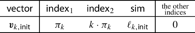
• 5. For each $q\in [Q_k]$, compute the following secret keys

  $$\begin{aligned} \textsf{IPFE}.\textsf{SK}_{k,q}&\leftarrow \textsf{IPFE}.\textsf {KeyGen}(\textsf{IPFE}.\textsf{MSK}, [\![\varvec{v}_{k,q}]\!]_2), \qquad \text {and} \\ \widetilde{\textsf{IPFE}.\textsf{SK}}_{k,q}&\leftarrow \textsf{IPFE}.\textsf {KeyGen}(\textsf{IPFE}.{\widetilde{\textsf {MSK}}}, [\![\widetilde{\varvec{v}}_{k,q}]\!]_2), \end{aligned}$$

  where the vectors $\varvec{v}_{k,q}, \widetilde{\varvec{v}}_{k,q}$ are defined as follows:

  

  

  Note that, the random vector $\varvec{s}_{\varvec{x}}$ has already been sampled during encryption.

Finally, it returns the simulated secret key as

$$\begin{aligned} \textsf{SK}_{(\varvec{M},\mathcal {I}_{\varvec{M}})} = \left( (\varvec{M},\mathcal {I}_{\varvec{M}}), \Big \{\textsf{IPFE}.\textsf{SK}_{k, \textsf{init}}, \big \{\textsf{IPFE}.\textsf{SK}_{k,q}, \widetilde{\textsf{IPFE}.\textsf{SK}}_{k,q}\}_{q\in [Q_k]}\Big \}_{k\in \mathcal {I}_{\varvec{M}}}\right) . \end{aligned}$$

We will use the following lemmas in our security analysis.

Lemma 4

Let $\textsf{IPFE}= (\textsf {Setup}, \textsf {KeyGen}, \textsf {Enc}, \textsf {Dec})$ be a function hiding inner product encryption scheme. For any polynomial $m = m(\lambda )$ and $n = n(\lambda )$ with $m > n$, define the following vectors

Then, for any $\textsf{IPFE}.\textsf{MSK}\leftarrow \textsf{IPFE}.\textsf {Setup}(1^{\lambda }, 1^*)$, the distributions $\{ \{\textsf{IPFE}.\textsf{SK}_{k}\}_{k \in [n]}, \{\textsf{IPFE}.\textsf{SK}_{k}^{(\mathfrak {b})}\}_{k \in [n+1, m]} , \{\textsf{IPFE}.\textsf{CT}_{k'}\}_{k' \in [n]} \}$ for $\mathfrak {b} \in \{0, 1\}$ are indistinguishable where

Proof

We prove this lemma by the transformation $\widehat{\pi }_k = \pi _k - \frac{\widehat{r}_k}{\rho _{k'}(k-k')}$ for $k \ne k'$. Note that $\widehat{\pi }_k$ is uniform over $\mathbb {Z}_p$ since $\pi _k \leftarrow \mathbb {Z}_p$. The lemma follows from the function hiding security of $\textsf{IPFE}$ since

$$\begin{aligned} {\varvec{v}^{(0)}} \cdot {\varvec{u}_{k'}}&= \pi _k\rho _{k'} \cdot (k-k') + r_k\\&= \Bigg (\widehat{\pi }_k + \frac{\widehat{r}_k}{\rho _{k'}(k-k')}\Bigg ) \rho _{k'} \cdot (k-k') + r_k\\&= \widehat{\pi }_k\rho _{k'} \cdot (k-k') + r_k + \widehat{r}_k = {\varvec{v}^{(1)}} \cdot {\varvec{u}_{k'}} \end{aligned}$$

Firstly, we note that the distributions of $\widehat{\pi }_k$ and $\pi _k$ are statistically close. Secondly, we note that the inner product value ${\varvec{v}^{(\mathfrak {b})}} \cdot {\varvec{u}_{k'}}$ remains the same for $\mathfrak {b} \in \{0, 1\}$. Therefore, in the first step, we switch $\pi _k$ to $\widehat{\pi }_k$, where the two distributions are statistically close. Then, in the second step, we utilize the function hiding property to switch the vector from $\varvec{v}^{(0)}$ to $\varvec{v}^{(1)}$. $\square$

Theorem 3

Assuming the $\textsf{SXDH}$ assumption holds in $\mathcal {G}$ and the $\textsf{IPFE}$ is function hiding secure, the above construction of $(1\textsf {-}\textsf{SK}, 1\textsf {-}\textsf{CT}, 1\textsf {-Slot})\textsf {-FE}$ for $\textsf{UAWS}$ is adaptively simulation secure.

Proof idea Before going for a formal proof, we discuss a high level overview of the proof. We use a three-step approach and each step consists of a group of hybrid sequence.

• In the first step, the label function $\ell _{k, \textsf{init}}$ is reversely sampled with the value $\varvec{z}[k]M_k[\varvec{x}] + \beta _k$ and it is hardwired in either $\varvec{u}_{k, \textsf{init}}$ or $\varvec{v}_{k, \textsf{init}}$, whichever is computed later.

• The second step is a loop. The purpose of the loop is to change all the honest label values $\ell _{k, t, i, j, \varvec{W}, q}$ to simulated ones that take the form $\ell _{k, t, i, j, \varvec{W}, q} = \varvec{s}_{\varvec{x}}[(t,i,j,\varvec{W})]\varvec{s}_{k, f}[q]$ where $\varvec{s}_{\varvec{x}}[(t,i,j,\varvec{W})]$ is hardwired in $\varvec{u}_{k, t, i, j, \varvec{W}}$ or $\widetilde{\varvec{u}}_{k, T+1, i, j, \varvec{W}}$ and $\varvec{s}_{k, f}[q]$ is hardwired in $\varvec{v}_{k,q}$ or $\widetilde{v}_{k, q}$. The procedure depends on the order of adversary’s queries.

• After all the label values $\ell _{k, t, i, j, \varvec{W}, q}$ are simulated, the third step uses a few more hybrids to reversely sample $\ell _{1, \textsf{init}}$ and $\ell _{k, \textsf{init}}|_{k>1}$ with the hardcoded values $\varvec{M}(\varvec{x})^{\top } \varvec{z} + \beta _1$ and $\beta _k|_{k>1}$ respectively. We also rearrange the elements so that the distribution of the ciphertext does not change with the occurrence of the secret key whether it comes before or after the ciphertext.

Recall that the adversary is allowed to query only a single secret key either before ($\textsf{SK}$ before $\textsf{CT}$) or after ($\textsf{CT}$ before $\textsf{SK}$) the challenge ciphertext. Accordingly, we consider two different cases depending on the occurrence of the single secret key query.

${Case\,\textit{1} \,( \textsf{CT}\,\,before \,\,\textsf{SK}) :}$ In this case, we place the reversely sampled $\ell _{k, \textsf{init}}$ in the $\varvec{v}_{k, \textsf{init}}$ in the exponent of $\mathbb {G}_2$. The loop of the second step runs over $(k, t, i, j, \varvec{W})$ in lexicographical order. In each iteration, we clean $\varvec{u}_{k, t, i, j, \varvec{W}}$ and shift everything to $\varvec{v}_{k, q}$ in one step and truly randomize the label values using DDH in $\mathbb {G}_2$ and then change these to their simulated form $\ell _{k, t, i, j, \varvec{W}, q} = \varvec{s}_{\varvec{x}}[(t,i,j,\varvec{W})]\varvec{s}_{k, f}[q]$ by again using DDH in $\mathbb {G}_2$. Finally, the terms $\{\varvec{s}_{\varvec{x}}[(t,i,j,\varvec{W})]\}_{t \in [T+1]}$ are shifted back to $\varvec{u}_{k, t, i, j, \varvec{W}}$ or $\widetilde{\varvec{u}}_{k, T+1, i, j, \varvec{W}}$.

${\textit{Case 2 }( \textsf{SK}\,\, before \,\,\textsf{CT}) :}$ In this case, we place the reversely sampled $\ell _{k, \textsf{init}}$ in the $\varvec{u}_{k, \textsf{init}}$ in the exponent of $\mathbb {G}_1$. The second step involves a two-level loop with outer loop running over t in increasing order and inner loop running over q in increasing order. In each iteration of the loop, we move all occurrences of $\varvec{r}_{k, f}[q]$ and $\varvec{s}_{k, f}[q]$ into all $\varvec{u}_{k, t', i^{\prime }, j^{\prime }, \varvec{W}^{\prime }}$ in one shot and hardwire the honest labels $\ell _{k, t, i, j, \varvec{W}, q}$ into $\varvec{u}_{k, t, i, j, \varvec{W}}$ for all $i, j, \varvec{W}$. Next, by invoking DDH in $\mathbb {G}_1$, we first make the honest labels $\ell _{k, t, i, j, \varvec{W}, q}$ truly random for all $i, j, \varvec{W}$ and then transform these into their simulated form $\ell _{k, t, i, j, \varvec{W}, q} = \varvec{s}_{\varvec{x}}[(t,i,j,\varvec{W})]\varvec{s}_{k, f}[q]$ again by using DDH in $\mathbb {G}_1$ for all $i, j, \varvec{W}$. Finally, the terms $\varvec{s}_{k, f}[q]$ are shifted back to $\varvec{v}_{k, q}$ or $\widetilde{\varvec{v}}_{k, q}$.

We start the formal proof with the first step where both the cases can be handled together. The next two steps are managed separately according to the occurrence of the secret key. We also note that the advantage of the adversary $\mathcal {A}$ in distinguishing any two consecutive hybrids depends on either the computational hardness of the function hiding security of IPFE or the harness of the DDH assumption in source groups. Moreover, there are a few hybrids that are either identically distributed with each other or the indistinguishability follows from the security of AKGS which is an information-theoretic tool. Since there are only a polynomial number of hybrids the total advantage of the adversary in breaking the security of UAWS is bounded by a polynomial ($\textsf{poly}(n_{\textsf {max}}, T, N, S, 2^{S}, Q)$) multiplied with the advantage of an adversary in breaking function hiding security of IPFE and the hardness of the DDH assumptions in the source groups. We observe that the term $2^S$ remains polynomial in the security parameter for logspace Turing machines. Therefore, the security of our UAWS can be reduced to the (polynomial) security of IPFE and the hardness of the SXDH assumption.

Proof

Let $\mathcal {A}$ be a PPT adversary in the security experiment of $\textsf{UAWS}$. We show that the advantage of $\mathcal {A}$ in distinguishing between the experiments $\textsf {Expt}_{\mathcal {A}, \textsf {real}}^{1\textsf {-}\textsf{UAWS}}(1^{\lambda })$ and $\textsf {Expt}_{\mathcal {A}, \textsf {ideal}}^{1\textsf {-}\textsf{UAWS}}(1^{\lambda })$ is negligible. In this security analysis, we additionally assume that the adversary can query only a single secret key for $(\varvec{M}, \mathcal {I}_{\varvec{M}})$ either before or after the challenge ciphertext. Let $((\varvec{x}, 1^{T}, 1^{2^{S}}), \varvec{z})$ be the challenge message and $\varvec{z} \in \mathbb {Z}_p^n$. We also assume that the single key queried by the adversary cover all the indices of the ciphertexts, i.e., $\mathcal {I}_{\varvec{M}}\supseteq [n]$ which is natural as the adversary gets maximum information about the ciphertext in such case. Without loss of generality and for the simplicity of exposition, we assume that the number of states in all Turing machines is the same and it is Q.

The first few hybrids are the same for both the cases: $\textsf{CT}$ before $\textsf{SK}$ and $\textsf{SK}$ before $\textsf{CT}$. The indistinguishability arguments remain unchanged in such hybrids. In Table 3, we represent the first/last few hybrids. Let $n_{\textsf {max}}$ be the maximum value of n, the length of $\varvec{z}$, i.e., $\mathcal {A}$ can choose the private attribute whose maximum length can be $n_{\textsf {max}}$.

Hybrid $\textsf {H}_0$. This is the real experiment $\textsf {Expt}_{\mathcal {A}, \textsf {real}}^{1\textsf {-}\textsf{UAWS}}(1^{\lambda })$ ($= \textsf {H}_{\textsf {real}}$ in Table 3) where the ciphertext vectors contains the challenge message $(\varvec{x}, \varvec{z})$ and the secret key vectors are computed using $(\varvec{M}, \mathcal {I}_{\varvec{M}})$.

Hybrid $\textsf {H}_{0.1}$. At the beginning of the experiment, the challenger samples an integer $n' \leftarrow [n_{\textsf {max}}]$ as a guess of n. This hybrid is exactly the real experiment except the challenger aborts the experiment immediately if the vector length of $\varvec{z}$ is not $n'$, i.e., $n \ne n'$. Suppose $\mathcal {A}$ outputs $\perp$ when the experiment is aborted. Thus, it is easy to see that the advantage of $\mathcal {A}$ in $\textsf {H}_{0.1}$ is $\frac{1}{n_{\textsf {max}}}$ times the advantage in $\textsf {H}_0$. Thus, if the advantage of $\mathcal {A}$ is negligible in $\textsf {H}_0$, then it is so in $\textsf {H}_{0.1}$. Hence, in the remaining hybrids we simply write $n' = n$.

Hybrid $\textsf {H}_{0.2}$. It proceeds exactly the same as $\textsf {H}_{0.1}$ except that if the queried key $(\varvec{M}, \mathcal {I}_{\varvec{M}})$ is such that $(\text {max } \mathcal {I}_{\varvec{M}}> n) \wedge (\text {min } \mathcal {I}_{\varvec{M}}\le n)$, then $\beta _k = \varvec{v}_{k, \textsf{init}}[\textsf{acc}]$ is replaced with $\widehat{\beta }_k \leftarrow \mathbb {Z}_p$ for each $k \in \mathcal {I}_{\varvec{M}}$. Thus, with high probability it holds that $\sum _{k \in \mathcal {I}_{\varvec{M}}} \widehat{\beta }_k \ne 0$. The hybrids $\textsf {H}_{0.1}$ and $\textsf {H}_{0.2}$ are indistinguishable by the function hiding security of $\textsf{IPFE}$ via the Lemma 4. Note that in this hybrid, we crucially use the randomness of the positions $\varvec{v}_{k, \textsf{init}}[\textsf{index}_1]$ and $\varvec{v}_{k, \textsf{init}}[\textsf{index}_2]$ (encoding the indices which are not available in the ciphertext vectors) to sample $\widehat{\beta }_k$ independently from other indices of the secret key.

Hybrid $\textsf {H}_1$. It proceeds exactly the same as $\textsf {H}_{0.2}$ except $\ell _{k, \textsf{init}}$ is hardwired in $\varvec{v}_{k, \textsf{init}}$ or $\varvec{u}_{k, \textsf{init}}$, and $\varvec{s}_{k, f} \leftarrow \mathbb {Z}_p^Q, \varvec{s}_{\varvec{x}} \leftarrow \mathbb {Z}_p^{[T+1]\times [N]\times [S]\times \{0,1\}^{S}}$ are embedded in $\varvec{v}_{k, q}, \widetilde{\varvec{u}}_{k, T+1, i, j, \varvec{W}}$ respectively. The first change sets the stage for $\ell _{k, \textsf{init}}$ to be reversely sampled in the next hybrid and the second change prepares the $\ell _{k, t, i, j, \varvec{W}, q}|_{t\le T}, \ell _{k, T+1, i, j, \varvec{W}, q}$ to be simulated as pseudorandom values in the loop hybrids. More specifically, the changes are implemented as follows:

• For $\textsf{CT}\text { before }\textsf{SK}$, $\varvec{u}_{k, \textsf{init}}$ is set to 1 during encryption and $\varvec{v}_{k, \textsf{init}}$ is set to $\varvec{r}_{\varvec{x}}[(0, 1, 1, \varvec{0}_{S})]\varvec{r}_{k, f}[1]$ during key generation.

• For $\textsf{SK}\text { before }\textsf{CT}$, $\varvec{v}_{k, \textsf{init}}$ is set to 1 during key generation and $\varvec{u}_{k, \textsf{init}}$ is set to $\varvec{r}_{\varvec{x}}[(0, 1, 1, \varvec{0}_{S})] \varvec{r}_{k, f}[1]$ during encryption. Note that, $\varvec{r}_{k, f}[1]$s are known only for $k \in \mathcal {I}_{\varvec{M}}$. Thus, $\varvec{u}_{k, \textsf{init}}[\textsf{init}]$ is unchanged in this and in the rest of the hybrids for $k \in [n] \setminus \mathcal {I}_{\varvec{M}}$.

• Also, $\varvec{v}_{k, q}[\textsf{sim}]$ is set to $\varvec{s}_{k, f}[q]$ and $\widetilde{\varvec{u}}_{k, T+1, i, j, \varvec{W}}[\textsf{sim}]$ is set to $\varvec{s}_{\varvec{x}}[(T+1,i,j,\varvec{W})]$.

Note that, the inner products between $\varvec{v}$’s and $\varvec{u}$’s remain unchanged. Therefore, the function hiding property of $\textsf{IPFE}$ ensures that $\textsf {H}_0$ and $\textsf {H}_1$ are indistinguishable.

Hybrid $\textsf {H}_2$. It proceeds identically to $\textsf {H}_1$ except that $\ell _{k, \textsf{init}}$ is reversely sampled from the other labels. By the piecewise security of $\textsf{AKGS}$, the hybrids $\textsf {H}_1$ and $\textsf {H}_2$ are indistinguishable (Tables 1, 2).$\square$

Table 1 The initial few hybrids in the security proof of $1\textsf {-UAWS}$

Table 2 The last few hybrids in the security proof of $1\textsf {-UAWS}$

Table 3 The remaining note of the first/last few hybrids in the security proof of $1\textsf {-UAWS}$.

Hybrid $\textsf {H}_4$. It proceeds identically to $\textsf {H}_2$ except the inner products ${\varvec{u}_{k, t, i, j, \varvec{W}}} \cdot {\varvec{v}_{k, q}}$ and ${\widetilde{\varvec{u}}_{k, T+1, i, j, \varvec{W}}} \cdot {\widetilde{\varvec{v}}_{k, q}}$ change from the honest to simulated labels $\varvec{s}_{\varvec{x}}[(t,i,j,\varvec{W})]\varvec{s}_{k, f}[q]$ and $\varvec{s}_{\varvec{x}}[(T+1,i,j,\varvec{W})]\varvec{s}_{k, f}[q]$ respectively. This is implemented by clearing the values at $\textsf{rand}, \textsf{acc}, \textsf{tb}_{\tau }$ of the vectors $\varvec{u}_{k, t, i, j, \varvec{W}}, \widetilde{\varvec{u}}_{k, T+1, i, j, \varvec{W}}$ and embedding $\varvec{s}_{k, f}[q], \varvec{s}_{\varvec{x}}[(t,i,j,\varvec{W})]$ at $\widetilde{\varvec{v}}_{k, q}[\textsf{sim}], \varvec{u}_{k, t, i, j, \varvec{W}}[\textsf{sim}]$ respectively. We show the indistinguishability between the hybrids $\textsf {H}_2$ and $\textsf {H}_3$ in two separate claims:

Claim 1

In the case of $\textsf{CT}\text { before }\textsf{SK}$, $\textsf {H}_2 \approx \textsf {H}_4$.

Claim 2

In the case of $\textsf{SK}\text { before }\textsf{CT}$, $\textsf {H}_2 \approx \textsf {H}_4$.

Hybrid $\textsf {H}_5$. It proceeds exactly the same as $\textsf {H}_4$ except the values at $\textsf{rand}, \textsf{acc}, \textsf{tb}_{\tau }$ of the vectors $\varvec{v}_{k, q}, \widetilde{\varvec{v}}_{k, q}$ are cleared and $\varvec{u}_{k, \textsf{init}}[\textsf{sim}]$ is set to 1. Also, for the case of $\textsf{CT}\text { before }\textsf{SK}$, $\ell _{k, \textsf{init}}$ is shifted from $\varvec{v}_{k, \textsf{init}}[\textsf{init}]$ to $\varvec{v}_{k, \textsf{init}}[\textsf{sim}]$. While the former change is common for both cases, the later prepares the ideal game for the case of $\textsf{CT}\text { before }\textsf{SK}$. Note that, the inner products between $\varvec{v}$’s and $\varvec{u}$’s remain unchanged. Therefore, the function hiding property of $\textsf{IPFE}$ ensures that $\textsf {H}_4$ and $\textsf {H}_5$ are indistinguishable.

Hybrid $\textsf {H}_6$. It is the same as $\textsf {H}_5$ except the hardcoded values used in the reverse sampling procedure while computing $\ell _{k, \textsf{init}}$ (for both cases). It computes $\ell _{k, \textsf{init}}$ as follows:

where all the other label values $\ell _{k, t, i, j, \varvec{W}, q} = \varvec{s}_{\varvec{x}}[(t,i,j,\varvec{W})]\varvec{s}_{k, f}[q]$ are already simulated. If the queried key satisfies the permissiveness, i.e., $\mathcal {I}_{\varvec{M}}\subseteq [n]$, then this is accomplished by a statistical transformation on $\{\beta _k: \beta _k \leftarrow \mathbb {Z}_p, \sum _{k \in \mathcal {I}_{\varvec{M}}} \beta _k = 0\}$. We replace $\beta _k$ by newly sampled $\beta _k$:

$$\begin{aligned} \beta _1&= \beta _1^{\prime } - \varvec{z}[1] M_1(\varvec{x}) + \varvec{M}(\varvec{x})^{\top } \varvec{z} \\ \beta _k&= \beta _k^{\prime } - \varvec{z}[k] M_k(\varvec{x}) ~~\text { for all }k>1 \end{aligned}$$

where $\beta _k^{\prime } \leftarrow \mathbb {Z}_p$. Observe that it still holds that $\sum _{k \in \mathcal {I}_{\varvec{M}}} \beta _k = 0$. On the other hand, if the key under consideration does not satisfy the permissiveness, i.e., $(\text {max~} \mathcal {I}_{\varvec{M}}> n) \wedge (\text {min ~}\mathcal {I}_{\varvec{M}}<n )$, then we know that $\widehat{\beta }_k$ are uniform over $\mathbb {Z}_p$. Thus, we can replace $\widehat{\beta }_k$ by new $\widehat{\beta }_k$:

$$\begin{aligned} \widehat{\beta }_1&= \beta _1^{\prime } - \varvec{z}[1] M_1(\varvec{x}) + \varvec{M}(\varvec{x})^{\top } \varvec{z} \\ \widehat{\beta }_k&= \beta _k^{\prime } - \varvec{z}[k] M_k(\varvec{x}) ~~\text { for all }k>1 \end{aligned}$$

where $\beta _k^{\prime } \leftarrow \mathbb {Z}_p$. Note that, the distributions of new $\beta _k$ or $\widehat{\beta }_k$ are statistically close to their old versions and hence the two hybrids $\textsf {H}_5$ and $\textsf {H}_6$ are indistinguishable.

Hybrid . This hybrid is equivalent to the ideal experiment $\textsf {Expt}_{\mathcal {A}, \textsf {ideal}}^{1\textsf {-}\textsf{UAWS}}(1^{\lambda })$ for the case of $\textsf{CT}\text { before }\textsf{SK}$. Thus, one should omit this hybrid in the case of $\textsf{SK}\text { before }\textsf{CT}$. In , the positions $\textsf{init}, \textsf{rand}, \textsf{acc}, \textsf{tb}_{\tau }$ of the vectors $\varvec{u}_{k, \textsf{init}}, \varvec{u}_{k, t, i, j, \varvec{W}}, \widetilde{\varvec{u}}_{k, T+1, i, j, \varvec{W}}$ are changed back to their normal form as they were in $\textsf {H}_0$ except we use an arbitrary vector $\varvec{\nu } \leftarrow \mathbb {Z}_p^n$ in place of $\varvec{z}$ (for $\widetilde{\varvec{u}}_{k, T+1, i, j, \varvec{W}}$). This change has no effect in the inner products between $\varvec{u}$’s and $\varvec{v}$’s since the corresponding terms in $\varvec{v}$’s are zero. The purpose of this change is to maintain the distribution of the ciphertext vectors consistent with the case of $\textsf{SK}\text { before }\textsf{CT}$. Finally, is indistinguishable from $\textsf {H}_6$ by the function hiding property of $\textsf{IPFE}$, and hence .

The sequence of hybrids for the case of $\textsf{CT}\text { before }\textsf{SK}$ ends here and the rest of the hybrids are required only to handle the case of $\textsf{SK}\text { before }\textsf{CT}$.

Hybrid $\textsf {H}_7$. It proceeds exactly the same as $\textsf {H}_6$ except it samples a dummy vector $\varvec{d} \leftarrow \mathbb {Z}_p^n$ such that

$$\begin{aligned} \varvec{M}(\varvec{x})^{\top } \varvec{z} = \varvec{M}(\varvec{x})^{\top } \varvec{d} = \sum _{k \in [n]} M_k(\varvec{x})\varvec{d}[k]. \end{aligned}$$

and reversely sample $\ell _{1, \textsf{init}}$ with the hardcoded value $\varvec{M}(\varvec{x})^{\top } \varvec{d} + \beta _1$ instead of $\varvec{M}(\varvec{x})^{\top } \varvec{z} + \beta _1$. Note that, this is statistical change to the computation of $\ell _{1, \textsf{init}}$, and hence the hybrids $\textsf {H}_6$ and $\textsf {H}_7$ are indistinguishable to the adversary.

Hybrid $\textsf {H}_{(7\rightarrow 0)}$. Next, for the case of $\textsf{SK}\text { before }\textsf{CT}$, we traverse in the reverse direction from $\textsf {H}_7$ to all the way to $\textsf {H}_0$ with the dummy vector $\varvec{d}$ in place of $\varvec{z}$. This step is inspired from the proof technique used by Datta and Pal [38]. We skip the descriptions of these hybrids as the indistinguishability arguments would be exactly similar to what we used for reaching $\textsf {H}_7$ from $\textsf {H}_0$. We denote the new $\textsf {H}_0$ as $\textsf {H}_{(7\rightarrow 0)}$ and the hybrids $\textsf {H}_7$ and $\textsf {H}_{(7\rightarrow 0)}$ are indistinguishable by the function hiding security of $\textsf{IPFE}$ and the piecewise security of $\textsf{AKGS}$. After this hybrid, observe that the reduction do not need to guess n which enables the final simulator to generate the pre-ciphertext secret key without any information about the length of private attribute $\varvec{z}$.

Hybrid . It is exactly the same as $\textsf {H}_{(7\rightarrow 0)}$ except the position $\textsf{sim}$ of the vectors $\varvec{u}_{k, \textsf{init}}, \varvec{u}_{k, t, i, j, \varvec{W}}$ and $\widetilde{\varvec{u}}_{k, T+1, i, j, \varvec{W}}$ are set as $1, \varvec{s}_{\varvec{x}}[(t,i,j,\varvec{W})]$ and $\varvec{s}_{\varvec{x}}[(T+1,i,j,\varvec{W})]$ respectively. Observe that this change has no effect in the inner product computation of these vectors with their corresponding vectors in the secret key as the positions in the secret key vectors are zero. This, however, keeps the ciphertext distribution consistent with the case of $\textsf{CT}\text { before }\textsf{SK}$. Therefore, and $\textsf {H}_{(7\rightarrow 0)}$ are indistinguishable by the function hiding security of the $\textsf{IPFE}$. We also note that is the ideal experiment $\textsf {Expt}_{\mathcal {A}, \textsf {ideal}}^{1\textsf {-}\textsf{UAWS}}(1^{\lambda })$ for the case of $\textsf{SK}\text { before }\textsf{CT}$, and hence . This completes the proof. $\square$ $\square$

Proof of Claim 1

For the case of $\textsf{CT}\text { before }\textsf{SK}$, we prove $\textsf {H}_2 \approx \textsf {H}_4$ using a sequence of hybrids $\textsf {H}_{3, t, i, j, \varvec{W}, 1}, \ldots , \textsf {H}_{3, t, i, j, \varvec{W}, 5}$ for $(t, i, j, \varvec{W}) \in [T]\times [N] \times [S] \times \{0, 1\}^{S}$ in lexicographical order. These hybrids are described in Table 4. Then, we use another sequence of hybrids (dedicated for the second $\textsf{IPFE}$) $\widetilde{\textsf {H}}_3, \widetilde{\textsf {H}}_{3, i, j, \varvec{W}, 1}, \ldots , \widetilde{\textsf {H}}_{3, i, j, \varvec{W}, 5}$ for $(t, i, j, \varvec{W}) \in [T]\times [N] \times [S] \times \{0, 1\}^{S}$ in lexicographical order. These hybrids are illustrated in Table 5. We denote by $(t, i, j, \varvec{W}) + 1$ the next tuple of indices in increasing order. We observe that $\varvec{u}$’s are listed before $\varvec{v}$’s since in the case of $\textsf{CT}\text { before }\textsf{SK}$ the ciphertext appears before the secret key.

Table 4 The loop hybrids for $t \le T$ in the security proof of $1\textsf {-UAWS}$ for the case where the ciphertext challenge comes before the secret key query

Table 5 The hybrid $\widetilde{\textsf {H}}_3$ followed by the loop hybrids in the security proof of $1\textsf {-UAWS}$ for the case where the ciphertext challenge comes before the secret key query

Hybrid $\textsf {H}_{3, t, i, j, \varvec{W}, 1}$. It proceeds identically to $\textsf {H}_2$ except that for all $(t', i^{\prime }, j^{\prime }, \varvec{W}^{\prime }) < (t, i, j, \varvec{W})$, $\varvec{u}_{k, t', i^{\prime }, j^{\prime }, \varvec{W}^{\prime }}$ has its values in $\textsf{rand}$ and $\textsf{tb}_{\tau }$’s cleared, and that a random value $\varvec{s}_{\varvec{x}}[(t',i^{\prime },j^{\prime },\varvec{W}^{\prime })]$ is embedded in $\varvec{u}_{k, t', i^{\prime }, j^{\prime }, \varvec{W}^{\prime }}[\textsf{sim}]$. This means that all the labels for $(t', i^{\prime }, j^{\prime }, \varvec{W}^{\prime })< (t, i, j, \varvec{W})$ are simulated, the first label $\ell _{k, \textsf{init}}$ is reversely sampled and the rest are honestly computed.

Hybrid $\textsf {H}_{3, t, i, j, \varvec{W}, 2}$. It proceeds exactly the same way as $\textsf {H}_{3, t, i, j, \varvec{W}, 1}$ except that the values in $\varvec{u}_{k, t, i, j, \varvec{W}}$ are set to zero and its inner product with $\varvec{v}_{k, q}$’s, i.e. the labels $\ell _{k, t, i, j, \varvec{W}, q}$ for all k, q, are hardcoded into $\varvec{v}_{k, q}$’s as follows:

• The positions $\textsf{rand}$ and $\textsf{tb}_{\tau }$ of $\varvec{u}_{k, t, i, j, \varvec{W}}$ are set to 0.

• The value at $\varvec{u}_{k, t, i, j, \varvec{W}}[\textsf{sim}^{\textsf{temp}}]$ is set to 1.

• The honest labels $\ell _{k, t, i, j, \varvec{W}, q} = -\varvec{r}_{\varvec{x}}[(t-1,i,j,\varvec{W})]\varvec{r}_{k, f}[q] + \cdots$ are embedded in $\varvec{v}_{k, q}[\textsf{sim}^{\textsf{temp}}]$ for each $q \in [Q]$ and $k \in \mathcal {I}_{\varvec{M}}$ where “$\cdots$” represents $\sum _{\tau \in \mathcal {T}}c_\tau (\varvec{x};t,i,j,\varvec{W};\varvec{r}_{\varvec{x}})({{\textbf {M}}}_{k,\tau }\varvec{r}_{k,f})[q]$.

As one can verify that the inner products between the vectors are unchanged, the indistinguishability between the hybrids $\textsf {H}_{3, t, i, j, \varvec{W}, 1}$ and $\textsf {H}_{3, t, i, j, \varvec{W}, 2}$ is guaranteed by the function hiding security of $\textsf{IPFE}$.

Hybrid $\textsf {H}_{3, t, i, j, \varvec{W}, 3}$. It proceeds similar to $\textsf {H}_{3, t, i, j, \varvec{W}, 2}$ except that the labels $\ell _{k, t, i, j, \varvec{W}, q}$ are changed to truly randomized values. We can invoke DDH assumption in $\mathbb {G}_2$ between the hybrids since the random values $\varvec{r}_{\varvec{x}}[(t-1,i,j,\varvec{W})]$ and $\varvec{r}_{k, f}[q]$’s only appear in the exponent of $\mathbb {G}_2$: for each $k \in \mathcal {I}_{\varvec{M}}$, given an $\textsf {MDDH}_{1, q}$ challenge

$\begin{array}{l} [\![\varvec{r}_{k, f}[1], \ldots , \varvec{r}_{k, f}[Q]; \varDelta _{k, 1}, \ldots , \varDelta _{k, Q}]\!]_2 : \\ \varDelta _{k, q} {\left\{ \begin{array}{ll} = \varvec{r}_{\varvec{x}}[(t-1,i,j,\varvec{W})]\varvec{r}_{k, f}[q], &{}\text {if \textsf {DDH} tuple} \\ \leftarrow \mathbb {Z}_p, &{} \text {if truly random tuple}\end{array}\right. } \end{array}$

we compute the labels as $\ell _{k, t, i, j, \varvec{W}, q} = -\varDelta _{k, q} + \cdots$. If a DDH tuple is received, the labels use pseudorandom randomizers $\varvec{r}_{t-1}[(i, j, \varvec{W}, \textvisiblespace )] = \varvec{r}_{\varvec{x}}[(t-1,i,j,\varvec{W})]\varvec{r}_{k, f}[q]$ as in $\textsf {H}_{3, t, i, j, \varvec{W}, 2}$. If a truly random tuple is received, these label values are truly random randomizers $\varvec{r}_{t-1}[(i, j, \varvec{W}, \textvisiblespace )] \leftarrow \mathbb {Z}_p^Q$ as in $\textsf {H}_{3, t, i, j, \varvec{W}, 3}$ due to the special piecewise security of $\textsf{AKGS}$. Note that, the values $[\![\ell _{k, \textsf{init}}]\!]_2 \leftarrow \textsf {RevSamp}(\cdots )$ can be efficiently computed in the exponent of $\mathbb {G}_2$.

Table 6 The outer loop hybrids running from $t = 1$ to T in the security proof of $1\textsf {-UAWS}$ for the case where the ciphertext challenge comes after the secret key query

Hybrid $\textsf {H}_{3, t, i, j, \varvec{W}, 4}$. It proceeds identical to $\textsf {H}_{3, t, i, j, \varvec{W}, 3}$ except the truly random labels $\ell _{k, t, i, j, \varvec{W}, q}$ for all $q\in [Q], k \in \mathcal {I}_{\varvec{M}}$ are replaced by pseudorandom values $\varvec{s}_{\varvec{x}}[(t,i,j,\varvec{W})]\varvec{s}_{k, f}[q]$ with $\varvec{s}_{\varvec{x}}[(t,i,j,\varvec{W})] \leftarrow \mathbb {Z}_p$. The hybrids $\textsf {H}_{3, t, i, j, \varvec{W}, 3}$ and $\textsf {H}_{3, t, i, j, \varvec{W}, 4}$ are indistinguishable due to the DDH assumption in $\mathbb {G}_2$ (the argument is similar to that of in the previous hybrid).

Hybrid $\textsf {H}_{3, t, i, j, \varvec{W}, 5}$. It proceeds exactly the same way as $\textsf {H}_{3, t, i, j, \varvec{W}, 4}$ except the pseudorandom labels $\ell _{k, t, i, j, \varvec{W}, q} = \varvec{s}_{\varvec{x}}[(t,i,j,\varvec{W})]\varvec{s}_{k, f}[q]$ hardwired in $\varvec{v}_{k, q}[\textsf{sim}^{\textsf{temp}}]$’s are split into $\varvec{u}_{k, t, i, j, \varvec{W}}[\textsf{sim}]$ (embedding the factor $\varvec{s}_{\varvec{x}}[(t,i,j,\varvec{W})]$) and $\varvec{v}_{k, q}[\textsf{sim}]$’s (embedding the factor $\varvec{s}_{k, f}[q]$). The inner products in the hybrids $\textsf {H}_{3, t, i, j, \varvec{W}, 4}$ and $\textsf {H}_{3, t, i, j, \varvec{W}, 5}$ are unchanged and hence the these two hybrids are indistinguishable due to the function hiding security of $\textsf{IPFE}$. Moreover, it can be observed that $\textsf {H}_{3, t, i, j, \varvec{W}, 5} \equiv \textsf {H}_{3, t', i', j', \varvec{W}', 3}$ for $(t', i^{\prime }, j^{\prime }, \varvec{W}^{\prime }) = (t, i, j, \varvec{W})+1$.

Therefore, in this sequence of hybrids for $t \le T$, we have $\textsf {H}_{3, 1, 1, 1, {{\textbf {0}}}_S, 1} \approx \textsf {H}_{3, T, N, S, {{\textbf {1}}}_S, 5}$. Now, we move to the next sequence of hybrids for $t = T+1$ as depicted in Table 5.

Hybrid $\widetilde{\textsf {H}}_3$. It is identical to $\textsf {H}_{3, T, N, S, {{\textbf {1}}}_S, 5}$ except the position $\textsf{sim}$ of $\widetilde{\varvec{u}}_{k, T+1, i, j, \varvec{W}}$ is zeroed out and $\widetilde{\varvec{v}}_{k, q}[\textsf{sim}]$ is set to $\varvec{s}_{k, f}[q]$ for all $k \in \mathcal {I}_{\varvec{M}}$. The inner products between the vectors are unchanged in $\textsf {H}_{3, T, N, S, {{\textbf {1}}}_S, 5}$ and $\widetilde{\textsf {H}}_3$. Thus, the indistinguishability between these two hybrids is ensured by the function security of $\textsf{IPFE}$.

Hybrid $\widetilde{\textsf {H}}_{3, i, j, \varvec{W}, 1}$. It proceeds identically to $\widetilde{\textsf {H}}_3$ except that for all $(i', j', \varvec{W}') < (i, j, \varvec{W})$, $\widetilde{\varvec{u}}_{k, T+1, i^{\prime }, j^{\prime }, \varvec{W}^{\prime }}$ has its values in $\textsf{rand}$ and $\textsf{acc}$’s cleared, and that a random value $\varvec{s}_{\varvec{x}}[(T+1,i^{\prime },j^{\prime },\varvec{W}^{\prime })]$ is embedded in $\widetilde{\varvec{u}}_{k, T+1, i^{\prime }, j^{\prime }, \varvec{W}^{\prime }}[\textsf{sim}]$.

Hybrid $\widetilde{\textsf {H}}_{3, i, j, \varvec{W}, 2}$. It proceeds exactly the same way as $\widetilde{\textsf {H}}_{3, i, j, \varvec{W}, 1}$ except that the values in $\widetilde{\varvec{u}}_{k, t, i, j, \varvec{W}}$ are set to zero and its inner product with $\widetilde{\varvec{v}}_{k, q}$’s, i.e. the labels $\ell _{k, T+1, i, j, \varvec{W}, q}$ for all k, q, are hardcoded into $\widetilde{\varvec{v}}_{k, q}$’s as follows:

• The positions $\textsf{rand}$ and $\textsf{acc}$ of $\widetilde{\varvec{u}}_{k, T+1, i, j, \varvec{W}}$ are set to 0.

• The value at $\widetilde{\varvec{u}}_{k, T+1, i, j, \varvec{W}}[\textsf{sim}^{\textsf{temp}}]$ is set to 1.

• The honest labels $\ell _{k, T+1, i, j, \varvec{W}, q} = -\varvec{r}_{\varvec{x}}[(T,i,j,\varvec{W})]\varvec{r}_{k, f}[q] + \cdots$ are embedded in $\widetilde{\varvec{v}}_{k, q}[\textsf{sim}^{\textsf{temp}}]$ for each $q \in [Q]$ and $k \in \mathcal {I}_{\varvec{M}}$ where ”$\cdots$“ represents the term $\varvec{y}_{k}[q]\varvec{z}[k]$.

The inner products between the vectors are unchanged, and hence the indistinguishability between the hybrids $\widetilde{\textsf {H}}_{3, i, j, \varvec{W}, 1}$ and $\widetilde{\textsf {H}}_{3, i, j, \varvec{W}, 2}$ is guaranteed by the function hiding security of $\textsf{IPFE}$.

Hybrid $\widetilde{\textsf {H}}_{3, i, j, \varvec{W}, 3}$. It proceeds similar to $\widetilde{\textsf {H}}_{3, i, j, \varvec{W}, 2}$ except that the labels $\ell _{k, T+1, i, j, \varvec{W}, q}$ are changed to truly randomized values. We can invoke DDH assumption in $\mathbb {G}_2$ as before to show the indistinguishability between the hybrids $\widetilde{\textsf {H}}_{3, i, j, \varvec{W}, 2}$ and $\widetilde{\textsf {H}}_{3, i, j, \varvec{W}, 3}$ since the random values $\varvec{r}_{\varvec{x}}[(T,i,j,\varvec{W})]$ and $\varvec{r}_{k, f}[q]$’s only appear in the exponent of $\mathbb {G}_2$ and hence the label functions can be truly randomized due to the special piecewise security of $\textsf{AKGS}$. Note that, the values $[\![\ell _{k, \textsf{init}}]\!]_2 \leftarrow \textsf {RevSamp}(\cdots )$ can be efficiently computed in the exponent of $\mathbb {G}_2$.

Hybrid $\widetilde{\textsf {H}}_{3, i, j, \varvec{W}, 4}$. It proceeds identical to $\widetilde{\textsf {H}}_{3, i, j, \varvec{W}, 3}$ except the truly random labels $\ell _{k, T+1, i, j, \varvec{W}, q}$ for all $q\in [Q], k \in \mathcal {I}_{\varvec{M}}$ are replaced by pseudorandom values $\varvec{s}_{\varvec{x}}[(T+1,i,j,\varvec{W})]\varvec{s}_{k, f}[q]$. The hybrids $\widetilde{\textsf {H}}_{3, i, j, \varvec{W}, 3}$ and $\widetilde{\textsf {H}}_{3, i, j, \varvec{W}, 4}$ are indistinguishable due to the DDH assumption in $\mathbb {G}_2$.

Hybrid $\widetilde{\textsf {H}}_{3, i, j, \varvec{W}, 5}$. It proceeds exactly the same way as $\widetilde{\textsf {H}}_{3, i, j, \varvec{W}, 4}$ except the pseudorandom labels $\ell _{k, T+1, i, j, \varvec{W}, q} = \varvec{s}_{\varvec{x}}[(T+1,i,j,\varvec{W})]\varvec{s}_{k, f}[q]$ hardwired in $\widetilde{\varvec{v}}_{k, q}[\textsf{sim}^{\textsf{temp}}]$’s are split into $\widetilde{\varvec{u}}_{k, T+1, i, j, \varvec{W}}[\textsf{sim}]$ (embedding the factor $\varvec{s}_{\varvec{x}}[(T+1,i,j,\varvec{W})]$) and $\widetilde{\varvec{v}}_{k, q}[\textsf{sim}]$’s (embedding the factor $\varvec{s}_{k, f}[q]$). The inner products in the hybrids $\widetilde{\textsf {H}}_{3, i, j, \varvec{W}, 4}$ and $\widetilde{\textsf {H}}_{3, i, j, \varvec{W}, 5}$ are unchanged and hence the these two hybrids are indistinguishable due to the function hiding security of $\textsf{IPFE}$. Moreover, it can be observed that $\widetilde{\textsf {H}}_{3, i, j, \varvec{W}, 5} \equiv \widetilde{\textsf {H}}_{3, i', j', \varvec{W}', 3}$ for $(i', j', \varvec{W}') = (i, j, \varvec{W}) +1$.

Therefore, in this sequence of hybrids for $t = T+1$, we have $\widetilde{\textsf {H}}_{3, 1, 1, {{\textbf {0}}}_S, 1} \approx \widetilde{\textsf {H}}_{3, N, S, {{\textbf {1}}}_S, 5}$. Lastly, we observe that $\widetilde{\textsf {H}}_{3, N, S, {{\textbf {1}}}_S, 5} \equiv \textsf {H}_4$ and hence $\textsf {H}_2 \approx \textsf {H}_4$ for the case of $\textsf{CT}\text { before }\textsf{SK}$. $\square$

Table 7 The inner loop hybrids in the security proof of 1-UAWS for the case where the ciphertext challenge comes after the secret key query

Table 8 The inner loop hybrids in the security proof of 1-UAWS for the case where the ciphertext challenge comes after the secret key query

Table 9 Table 5: the remaining notes

Table 10 The hybrid $\widetilde{\textsf {H}}_3$ followed by the loop hybrids and $\widetilde{\textsf {H}}_4$ in the security proof of $1\textsf {-UAWS}$ for the case where the ciphertext challenge comes after the secret key query

Proof of Claim 2

The case of $\textsf{SK}\text { before }\textsf{CT}$ for showing $\textsf {H}_2 \approx \textsf {H}_4$ is more involved and further difficulties arises since we have two independent $\textsf{IPFE}$s for each Turing machine in contrast to the security analysis of [62] where only a single $\textsf{IPFE}$ was sufficient.

The overall goal of the claim is to make all the label values $\ell _{k, t, i, j, \varvec{W}, q}$ simulated by invoking $\textsf {DDH}$ similar to the case of $\textsf{CT}\text { before }\textsf{SK}$. However, since the secret key comes before the challenge ciphertext and $\ell _{k, \textsf{init}} \leftarrow \textsf {RevSamp}(\cdots )$ is computed while encryption, we can only apply DDH into the ciphertext vectors which are computed in the exponent of $\mathbb {G}_1$. Thus, we have to move $\varvec{r}_{k, f}[q]$ into the ciphertext vectors (Table 7). But, in this case, $\varvec{r}_{k, f}[q]$ of $\varvec{v}_{k, q}$ may appear in $({{\textbf {M}}}_{k, \tau }\varvec{r}_{k, f})[q']$ of any $\varvec{v}_{k, q'}$ depending on the transition block. Moreover, $\varvec{r}_{k, f}[q]$ also presents in $\widetilde{\varvec{v}}_{k, q}$ which are associated to second $\textsf{IPFE}$. Hence, in the security analysis, we must take care of the following facts:

• The special piecewise security can only be applied in the increasing order of t for changing $\ell _{k, t, i, j, \varvec{W}, q}$’s to their simulated form.

• More importantly, to simulate $\ell _{k, t, i, j, \varvec{W}, q}$ for $t \le T$, all occurrence of $\varvec{r}_{k, f}[q]$ must be in the ciphertext of both the $\textsf{IPFE}$. Also, we can not simulate $\ell _{k, T+1, i, j, \varvec{W}, q}$ (in the second $\textsf{IPFE}$) while simulating $\ell _{k, t', i, j, \varvec{W}, q}$ (in the first $\textsf{IPFE}$).

• There is not enough space in the ciphertext to embed all the $\varvec{r}_{k, f}[q]$’s at the same time for each $k \in \mathcal {I}_{\varvec{M}}$.

• The values $\varvec{r}_{k, f}[q]$ must not go away until all $\ell _{k, t, i, j, \varvec{W}, q}$’s are simulated. Indeed, $\varvec{r}_{k, f}[q]$ still resides in $\varvec{v}_{k, q'}$’s in $\textsf {H}_4$, the end hybrid of the claim.

To deal with all these facts, we employ a strategy inspired from the proof technique of [62] where they use a two-level loop over t, q with $t \le T$ and switch, in the increasing order of t, q, batches of $NS2^S$ label functions. That is, for fixed t, q and all $i, j, \varvec{W}$ and for all $k \in \mathcal {I}_{\varvec{M}}$, the batches of label values $\ell _{k, t, i, j, \varvec{W}, q}$ are simulated by moving $\varvec{r}_{k, f}[q]$’s back and forth in each iteration. More precisely, in each iteration of t, q, when moving $\varvec{r}_{k, f}[q]$ into the ciphertext vectors, we erase all its occurrence in the secret key vectors of both the $\textsf{IPFE}$ and must compensate some $\ell _{t', i, j, \varvec{W}, q'}$’s for their loss of $\varvec{r}_{k, f}[q]$ using the indices with superscript $\textsf {comp}$ in the case of $t' \le T$. Observe that, $\varvec{r}_{k, f}[q]$ only appears in the position $\textsf{rand}$ of $\widetilde{\varvec{v}}_{k, q}$ of the second $\textsf{IPFE}$. Thus, it is not required to compensate the loss of $\varvec{r}_{k, f}[q]$ in any other $\ell _{T+1, i, j, \varvec{W}, q'}$’s. However, $\varvec{r}_{k, f}[q]$ is still required to shift into the ciphertext vectors of the second $\textsf{IPFE}$. We use the indices with superscript temp to hardcode the honest label values of $\ell _{T+1, i, j, \varvec{W}, q}$ while running the loop over t, q with $t \le T$. Finally, after the two-level loop running over t, q with $t \le T$ ends, we erase $\varvec{r}_{k, f}[q]$ from $\varvec{v}_{k, q}$ and run a separate loop over q in the increasing order to simulate the labels $\ell _{T+1, i, j, \varvec{W}, q}$’s using the indices with superscript temp in the second $\textsf{IPFE}$.

We define modes of a label $\ell _{t', i, j, \varvec{W}, q'}$ for ease of understanding the loops used in this claim (Table 9). The definitions of modes are similar to what used by [62]. There are three orthogonal group of nodes:

• The first group is about the value of the label. A label is honest if its value $L_{t', i, j, \varvec{W}, q'}(\varvec{x})$ is computed using the garbling randomness $\varvec{r} = \varvec{r}_{\varvec{x}} \otimes \varvec{r}_f$. It is random if its value is sampled uniformly at random. It is simulated if its value is $\varvec{s}_{\varvec{x}}[(t',i,j,\varvec{W})]\varvec{s}_{k, f}[q']$.

• The second group is about where the terms $\varvec{r}_f$ and $\varvec{s}_f$ are placed while computing the labels using the $\textsf{IPFE}$s. A label is normal (this is the default) if $\varvec{r}_f, \varvec{s}_f$ are placed in the secret key. It is compensated if $\varvec{r}_f[q], \varvec{s}_f[q]$ are placed in the ciphertext while the other components of $\varvec{r}_f, \varvec{s}_f$ are still in the secret key (for simplicity, we note that this mode only appears in the first $\textsf{IPFE}$). It is hardwired if the value (in its entirety) is hardwired in the ciphertext (for simplicity, we note that this mode only appears to the labels with $t' = t, q' = q$).

• In the last group, a label is normal (default) if it is computed without indices with superscript $\textsf {temp}$. It is temporary if it is computed with indices having superscript temp.

As discussed above, the first loop of this claim is a two-level loop with outer loop running over $t = 1, \dots , T$ (provided in Table 6) and the inner loop running over $q = 1, \dots , Q$ (given in Table 8). We call this part 1 of the proof. The second loop runs over $q = 1, \dots , Q$ (described in Table 10) and it is dedicated for simulating the label values $\ell _{k, T+1, i, j, \varvec{W}, q}$ for all $k \in \mathcal {I}_{\varvec{M}}$.We call this part 2 of the proof. In this hybrids, the secret key vectors $\varvec{v}$’s appear before the ciphertext vectors $\varvec{u}$’s.

$\square$

Part 1 The sequence of hybrids in the two-level loop (with $t \le T, q\le Q$) and their indistinguishability arguments (Table 11).

Hybrid $\textsf {H}_{3, t, 1}$. It proceeds identically to $\textsf {H}_2$ except that for all $t' < t \le T$ and all $i, j, \varvec{W}$, the vectors $\varvec{u}_{k, t', i, j, \varvec{W}}$ have their values at $\textsf{rand}$ and $\textsf{tb}_{\tau }$’s cleared, and that a random value $\varvec{s}_{\varvec{x}}[(t',i,j,\varvec{W})]$ is embedded in $\varvec{u}_{k, t', i, j, \varvec{W}}[\textsf{sim}]$. This means that all the labels for $(t < t' \le T, i, j, \varvec{W})$ are simulated, the first label $\ell _{k, \textsf{init}}$ is reversely sampled and the rest are honestly computed.

Hybrid $\textsf {H}_{3, t, 2}$. It proceeds exactly the same way as $\textsf {H}_{3, t, 1}$ except that the modes of $\ell _{k, t, i, j, \varvec{W}, q}$’s (for all $i, j, \varvec{W}, q$ with $t \le T$) are changed to honest and temporary, and that a random value $\varvec{s}_{\varvec{x}}[(t,i,j,\varvec{W})]$ is embedded in $\varvec{u}_{k, t, i, j, \varvec{W}}[\textsf{sim}^{\textsf{temp}}]$ for all $i, j, \varvec{W}$. The change is implemented as follows:

• The positions $\textsf{rand}$ and $\textsf{tb}_{\tau }$ of $\varvec{u}_{k, t, i, j, \varvec{W}}$ are copied to the positions $\textsf{rand}^{\textsf{temp}}$ and $\textsf{tb}_{\tau }^{\textsf{temp}}$ respectively, and then the positions $\textsf{rand}$ and $\textsf{tb}_{\tau }$ are set to 0.

• The value at $\varvec{u}_{k, t, i, j, \varvec{W}}[\textsf{sim}^{\textsf{temp}}]$ is set to $\varvec{s}_{\varvec{x}}[(t,i,j,\varvec{W})]$. It sets the stage for the inner loop which will make the label values $\ell _{k, t, i, j, \varvec{W},q}$’s as simulated and temporary.

• The positions $\textsf{rand}$ and $\textsf{tb}_{\tau }$ of $\varvec{v}_{k, q}$ are copied to the positions $\textsf{rand}^{\textsf{temp}}$ and $\textsf{tb}_{\tau }^{\textsf{temp}}$ respectively.

As one can verify that the inner products between the vectors are unchanged, the indistinguishability between the hybrids $\textsf {H}_{3, t, 1}$ and $\textsf {H}_{3, t, 2}$ is guaranteed by the function hiding security of $\textsf{IPFE}$.

Table 11 The notes of Table 10

Hybrid $\textsf {H}_{3, t, 4}$. It proceeds identical to $\widetilde{\textsf {H}}_{3, t, 2}$ except that the modes of $\ell _{k, t, i, j, \varvec{W}, q}$’s (for all $i, j, \varvec{W}, q$ with $t \le T$) are changed from honest and temporary to simulated and temporary. This is implemented by $\varvec{v}_{k, q}$’s have their values cleared at $\textsf{rand}^{\textsf{temp}}$, $\textsf{tb}_{\tau }^{\textsf{temp}}$, and $\varvec{v}_{k, q}[\textsf{sim}^{\textsf{temp}}]$ is set to $\varvec{s}_{k, f}[q]$. We show that $\textsf {H}_{3, t, 2} \approx \textsf {H}_{3, t, 4}$ by a sequence of hybrids used by the inner loop.

Hybrid $\textsf {H}_{3, t, 5}$. It proceeds identical to $\widetilde{\textsf {H}}_{3, t, 4}$ except that the modes of $\ell _{k, t, i, j, \varvec{W}, q}$’s (for all $i, j, \varvec{W}, q$ with $t \le T$) are changed from simulated and temporary to simulated. Moreover, some clean-up work is done in preparation of the next iteration. The change is implemented as follows:

• The positions $\textsf{rand}^{\textsf{temp}}$, $\textsf{tb}_{\tau }^{\textsf{temp}}$ and $\textsf{sim}^{\textsf{temp}}$ of $\varvec{u}_{k, t, i, j, \varvec{W}}$ are set to 0.

• The value at $\varvec{u}_{k, t, i, j, \varvec{W}}[\textsf{sim}]$ is changed from 0 to $\varvec{s}_{\varvec{x}}[(t,i,j,\varvec{W})]$.

• The positions $\textsf{sim}^{\textsf{temp}}$ of $\varvec{v}_{k, q}$ is set to 0.

Since the inner products between the vectors $\varvec{u}$’s and $\varvec{v}$’s are unchanged, the indistinguishability between the hybrids $\textsf {H}_{3, t, 4}$ and $\textsf {H}_{3, t, 4}$ is ensured by the function hiding security of $\textsf{IPFE}$. We observe that $\textsf {H}_{3, 1, 1} \equiv \textsf {H}_2$ and $\textsf {H}_{3, t, 5} \equiv \textsf {H}_{3, t+1, 1}$.

Now, we discuss the hybrids of the inner loop running over $q = 1, \dots , Q$, which switches the mode of $\ell _{k, t, i, j, \varvec{W}, q}$ from honest and temporary to simulated and temporary.

Hybrid $\textsf {H}_{3, t, 3, q, 1}$. It proceeds identical to $\textsf {H}_{3, t, 2}$, except that for $q' < q$, all the $\varvec{v}_{k, q'}$ have their values at $\textsf{rand}^{\textsf{temp}}, \textsf{tb}_{\tau }^{\textsf{temp}}$’s cleared, and the value $\varvec{s}_{k, f}[q']$ is embedded at $\varvec{v}_{k, q'}[\textsf{sim}^{\textsf{temp}}]$. This means that the labels $\ell _{k, t, i, j, \varvec{W}, q'}$ for all $i, j, \varvec{W}$ with $t \le T$ and $q' < q$ have been changed from honest and temporary to simulated and temporary.

Hybrid $\textsf {H}_{3, t, 3, q, 2}$. It proceeds identical to $\textsf {H}_{3, t, 3, q, 1}$ except that all occurrence of $\varvec{r}_{k, f}[q]$ and $\varvec{s}_{k, f}[q]$ are moved from $\varvec{v}_{k, q'}$’s to $\varvec{u}_{k, t', i, j, \varvec{W}, q}$’s using the compensation identity (Notes of Tables 4, 8), for all $q'\ne q$. Further, to make $\widetilde{\varvec{v}}_{k, q}$ free of $\varvec{r}_{k, f}[q]$, it’s positions $\textsf{rand}, \textsf{acc}$ are set to zero and $\textsf{sim}^{\textsf{temp}}$ is set to 1, and the labels $\ell _{k, T+1, i, j, \varvec{W}, q}$’s are hardwired at $\textsf{sim}^{\textsf{temp}}$ of $\widetilde{\varvec{u}}_{k, T+1, i, j, \varvec{W}}$ (hence they are in honest and hardwired mode). Thus, the labels with $q' = q$ or $(T \ge ) t' > t$ or $q'>q$ are computed using the compensation identity on top of their existing mode, and the labels $\ell _{k, t, i, j, \varvec{W}, q}$ for all $i, j, \varvec{W}$ become honest and hardwired (more specifically, hardwired in $\varvec{u}_{k, t, i, j, \varvec{W}}[\textsf{sim}^{\textsf{comp}}]$). The inner products between $\varvec{u}, \widetilde{\varvec{u}}$’s and $\varvec{v}, \widetilde{\varvec{v}}$’s are unchanged due to these modifications. Hence, the indistinguishability between the hybrids $\textsf {H}_{3, t, 3, q, 1}$ and $\textsf {H}_{3, t, 3, q, 2}$ follows from the function hiding security of $\textsf{IPFE}$.

Hybrid $\textsf {H}_{3, t, 3, q, 3}$. It proceeds identical to $\textsf {H}_{3, t, 3, q, 2}$ except the labels $\ell _{k, t, i, j, \varvec{W}, q}$ (for all $i, j, \varvec{W}$ with $t \le T$) hardwired in $\varvec{u}_{k, t, i, j, \varvec{W}}[\textsf{sim}^{\textsf{comp}}]$ become random and hardwired. The hybrids $\textsf {H}_{3, t, 3, q, 2}$ and $\textsf {H}_{3, t, 3, q, 3}$ are indistinguishable by the DDH assumption in $\mathbb {G}_1$.

Hybrid $\textsf {H}_{3, t, 3, q, 4}$. It proceeds identical to $\textsf {H}_{3, t, 3, q, 3}$ except the labels $\ell _{k, t, i, j, \varvec{W}, q}$ (for all $i, j, \varvec{W}$ with $t \le T$) hardwired in $\varvec{u}_{k, t, i, j, \varvec{W}}[\textsf{sim}^{\textsf{comp}}]$ become simulated and hardwired, i.e. $\ell _{k, t, i, j, \varvec{W}, q} = \varvec{s}_{\varvec{x}}[(t,i,j,\varvec{W})]\varvec{s}_{k, f}[q]$. The hybrids $\textsf {H}_{3, t, 3, q, 3}$ and $\textsf {H}_{3, t, 3, q, 4}$ are again indistinguishable by the DDH assumption in $\mathbb {G}_1$.

Hybrid $\textsf {H}_{3, t, 3, q, 5}$. It proceeds identical to $\textsf {H}_{3, t, 3, q, 4}$ except that all occurrences of $\varvec{r}_{k, f}[q]$ and $\varvec{s}_{k, f}[q]$ are moved back to $\varvec{v}_{k, q}$’s, and in the second $\textsf{IPFE}$, all the vectors are restored back to their initial form, i.e. $\varvec{r}_{k, f}[q]$ is moved back to $\widetilde{\varvec{v}}_{k, q}$. Further, some clean-up work is done in order to prepare the vectors for the next iteration. The values at the position $\textsf{sim}^{\textsf{comp}}$ of the vectors $\varvec{v}_{k, q}$ and $\varvec{u}_{k, t, i, j, \varvec{W}}$ are cleared, which means that the labels lose their compensation mode and the labels $\ell _{k, t, i, j, \varvec{W}, q}$ (for all $i, j, \varvec{W}$ with $t\le T$) become simulated and temporary. Also, the values at the position $\textsf{sim}^{\textsf{temp}}$ of $\widetilde{\varvec{v}}_{k, q}$ and $\widetilde{\varvec{u}}_{k, T+1, i, j, \varvec{W}}$ are cleared, which in turn ensures that the labels $\ell _{k, T+1, i, j, \varvec{W}, q}$’s are changed from honest hardwired to honest mode. It is easy to see that inner products between $\varvec{u}, \widetilde{\varvec{u}}$’s and $\varvec{v}, \widetilde{\varvec{v}}$’s are unchanged, and hence the indistinguishability between the hybrids $\textsf {H}_{3, t, 3, q, 4}$ and $\textsf {H}_{3, t, 3, q, 5}$ follows from the function hiding security of $\textsf{IPFE}$. We observe that $\textsf {H}_{3, t, 3, q, 5} \equiv \textsf {H}_{3, t, 3, q+1, 1}$, and hence $\textsf {H}_{3, t, 2} \approx \textsf {H}_{3, t, 4}$ in the outer loop hybrids of Table 6.

Note that, the two-level loop ends with the hybrid $\textsf {H}_{3, T, 5}$ where the labels $\ell _{k, t, i, j, \varvec{W}, q}$ for all $t \le T$ and for all $i, j, \varvec{W}$ are simulated. We now go to the part 2 of the proof.

Part 2 The sequence of hybrids in the second loop running over $q = 1, \dots , Q$ (for simulating the labels associated to $t = T+1$) with two additional hybrids and their indistinguishability arguments.

Hybrid $\widetilde{\textsf {H}}_3$. It is identical to $\textsf {H}_{3, T, 5}$ except the positions $\textsf{rand}, \textsf{tb}_{\tau }$ of $\varvec{v}_{k, q}$ are set to zero (in the first $\textsf{IPFE}$), and the positions $\textsf{rand}, \textsf{acc}$ of the vectors $\widetilde{\varvec{v}}_{k, q}$’s and $\widetilde{\varvec{u}}_{k, T+1, i, j, \varvec{W}}$’s are copied to their counterparts with superscript temp. Moreover, the positions $\textsf{rand}, \textsf{acc}$ of $\widetilde{\varvec{u}}_{k, T+1, i, j, \varvec{W}}$’s are cleared, which means that the labels $\ell _{k, T+1, i, j, \varvec{W}, q}$’s are in honest and temporary mode. The inner products between $\varvec{u}, \widetilde{\varvec{u}}$’s and $\varvec{v}, \widetilde{\varvec{v}}$’s are unchanged, and hence the indistinguishability between the hybrids $\textsf {H}_{3, T, 5}$ and $\widetilde{\textsf {H}}_{3}$ is guaranteed by the function hiding security of $\textsf{IPFE}$.

Hybrid $\widetilde{\textsf {H}}_{3, q, 1}$. It proceeds identical to $\widetilde{\textsf {H}}_{3}$ except that for $q' < q$, all the $\widetilde{\varvec{v}}_{k, q'}$ have their values at $\textsf{rand}^{\textsf{temp}}, \textsf{acc}^{\textsf{temp}}$’s cleared, and the value $\varvec{s}_{k, f}[q']$ is embedded at $\widetilde{\varvec{v}}_{k, q'}[\textsf{sim}]$. This means that the labels $\ell _{k, T+1, i, j, \varvec{W}, q'}$ for all $i, j, \varvec{W}$ and $q' < q$ have been changed from honest and temporary to simulated.

Hybrid $\widetilde{\textsf {H}}_{3, q, 2}$. It proceeds identical to $\widetilde{\textsf {H}}_{3, q, 1}$ except that the positions $\textsf{rand}, \textsf{acc}, \textsf{rand}^{\textsf{temp}}, \textsf{acc}^{\textsf{temp}}$ of $\widetilde{\varvec{v}}_{k, q}$ are cleared and $\widetilde{\varvec{v}}_{k, q}[\textsf{sim}^{\textsf{temp}}]$ is set to 1. Further, the labels $\ell _{k, T+1, i, j, \varvec{W}, q}$ (for all $i, j, \varvec{W}$) are hardwired at $\textsf{sim}^{\textsf{temp}}$ of $\widetilde{\varvec{u}}_{k, T+1, i, j, \varvec{W}}$, which means the labels are in honest and hardwired mode. The inner products between $\widetilde{\varvec{u}}$’s and $\widetilde{\varvec{v}}$’s are unchanged due to these modifications. Hence, the indistinguishability between the hybrids $\widetilde{\textsf {H}}_{3, q, 1}$ and $\widetilde{\textsf {H}}_{3, q, 2}$ follows from the function hiding security of $\textsf{IPFE}$.

Hybrid $\widetilde{\textsf {H}}_{3, q, 3}$. It proceeds identical to $\widetilde{\textsf {H}}_{3, q, 2}$ except the labels $\ell _{k, T+1, i, j, \varvec{W}, q}$ (for all $i, j, \varvec{W}$) hardwired in $\widetilde{\varvec{u}}_{k, T+1, i, j, \varvec{W}}[\textsf{sim}^{\textsf{temp}}]$ become random and hardwired. The hybrids $\widetilde{\textsf {H}}_{3, q, 2}$ and $\widetilde{\textsf {H}}_{3, q, 3}$ are indistinguishable by the DDH assumption in $\mathbb {G}_1$.

Hybrid $\widetilde{\textsf {H}}_{3, q, 4}$. It proceeds identical to $\widetilde{\textsf {H}}_{3, q, 3}$ except the labels $\ell _{k, T+1, i, j, \varvec{W}, q}$ (for all $i, j, \varvec{W}$) hardwired in $\widetilde{\varvec{u}}_{k, T+1, i, j, \varvec{W}}[\textsf{sim}^{\textsf{temp}}]$ become simulated and hardwired, i.e. $\ell _{k, T+1, i, j, \varvec{W}, q} = \varvec{s}_{\varvec{x}}[(T+1,i,j,\varvec{W})]\varvec{s}_{k, f}[q]$. The hybrids $\widetilde{\textsf {H}}_{3, q, 3}$ and $\widetilde{\textsf {H}}_{3, q, 4}$ are again indistinguishable by the DDH assumption in $\mathbb {G}_1$.

Hybrid $\widetilde{\textsf {H}}_{3, q, 5}$. It proceeds identical to $\widetilde{\textsf {H}}_{3, q, 4}$ except that all occurrences of $\varvec{r}_{k, f}[q]$ and $\varvec{s}_{k, f}[q]$ are moved back to $\widetilde{\varvec{v}}_{k, q}$’s, and some clean-up work is done in order to prepare the vectors for the next iteration. The values at the position $\textsf{sim}^{\textsf{temp}}$ of the vectors $\widetilde{\varvec{v}}_{k, q}$ and $\widetilde{\varvec{u}}_{k, T+1, i, j, \varvec{W}}$ are cleared, which means that the labels $\ell _{k, T+1, i, j, \varvec{W}, q}$ (for all $i, j, \varvec{W}$) become simulated. It is easy to see that inner products between $\widetilde{\varvec{u}}$’s and $\widetilde{\varvec{v}}$’s are unchanged, and hence the indistinguishability between the hybrids $\widetilde{\textsf {H}}_{3, q, 4}$ and $\widetilde{\textsf {H}}_{3, q, 5}$ follows from the function hiding security of $\textsf{IPFE}$. We observe that $\widetilde{\textsf {H}}_{3, q, 5} \equiv \widetilde{\textsf {H}}_{3, q+1, 1}$.

Hybrid $\widetilde{\textsf {H}}_4$. It is identical to $\widetilde{\textsf {H}}_{3, Q, 5}$ except $\varvec{r}_{k, f}[q]$’s are put back to $\varvec{v}_{k, q}$’s and the positions $\textsf{rand}^{\textsf{temp}}, \textsf{acc}^{\textsf{temp}}$ of $\widetilde{\varvec{u}}_{k, T+1, i, j, \varvec{W}}$ are set to zero. The inner products between $\varvec{u}, \widetilde{\varvec{u}}$’s and $\varvec{v}, \widetilde{\varvec{v}}$’s are unchanged, and hence the indistinguishability between the hybrids $\widetilde{\textsf {H}}_{3, Q, 5}$ and $\widetilde{\textsf {H}}_{4}$ is guaranteed by the function hiding security of $\textsf{IPFE}$.

Lastly, we note that $\textsf {H}_{3, 1, 1} \equiv \textsf {H}_2$ and $\widetilde{\textsf {H}}_4 \equiv \textsf {H}_4$ (cf. Table 3). Therefore, $\textsf {H}_2 \approx \textsf {H}_4$ in the case of $\textsf{SK}\text { before }\textsf{CT}$. $\square$

6 1-Slot FE for unbounded AWS for $\textsf{L}$

In this section, we construct a public key 1-slot $\textsf{FE}$ scheme for the unbounded attribute-weighted sum functionality for $\textsf{L}$. The scheme satisfies the same properties as of the $\textsf{SK}\text {-}\textsf{U}\textsf{AWS}^\textsf{L}_{(1,1,1)}$. However, the public key scheme supports releasing polynomially many secret keys and a single challenge ciphertext, hence we denote the scheme as $\textsf {PK}\text {-}\textsf{U}\textsf{AWS}^\textsf{L}_{(\textsf{poly},1,1)}$.

Along with the $\textsf{AKGS}$ for $\text {Logspace Turing machines}$ we require a function-hiding slotted $\textsf{IPFE}= (\textsf{IPFE}.\textsf {Setup}, \textsf{IPFE}.\textsf {KeyGen}, \textsf{IPFE}.\textsf {Enc}, \textsf{IPFE}.\textsf {SlotEnc}, \textsf{IPFE}.\textsf {Dec})$ based on $\textsf{G}$, where $\textsf{G}=(\mathbb {G}_1, \mathbb {G}_2, \mathbb {G}_{T }, g_1, g_2, e)$ is pairing group tuple of prime order p.

6.1 The construction

We now describe the $\textsf {PK}\text {-}\textsf{U}\textsf{AWS}^\textsf{L}_{(\textsf {poly},1,1)} = (\textsf {Setup},\textsf {KeyGen}, \textsf {Enc},\textsf {Dec})$.

$\textsf {Setup}(1^\lambda )$::

On input the security parameter, fix a prime integer $p\in \mathbb {N}$ and define the slots for generating two pair of $\textsf{IPFE}$ master keys as follows:

$$\begin{aligned} \mathcal {S}_{\textsf{pub}} =&\left\{ \textsf{index}_1, \textsf{index}_2, \textsf{pad}, \textsf{init}^{\textsf {pub}}, \textsf{rand}^{\textsf {pub}}, \textsf{acc}^{\textsf {pub}}\right\} \cup \{\textsf{tb}_{\tau }^\textsf{pub}| \tau \in \mathcal {T}\}, \\ \mathcal {S}_{\textsf{copy}} =&\left\{ \textsf{init}^{\textsf {copy}}, \textsf{rand}^{\textsf {copy}}\right\} \cup \{\textsf{tb}_{\tau }^\textsf{copy}| \tau \in \mathcal {T}\}, \\ \mathcal {S}_{\textsf{priv}} =&~ \mathcal {S}_{\textsf{copy}} \cup \mathcal {S}_{1\textsf {-}\textsf{UAWS}} \cup \{\textsf{pad}^{\textsf{copy}}, \textsf{pad}^{\textsf{temp}}, \textsf{acc}^{\textsf {perm}}, \textsf{sim}^{\textsf{copy}}\},\\ \widetilde{\mathcal {S}}_{\textsf{pub}} =&\{\textsf{index}_1, \textsf{index}_2, \textsf{rand}^{\textsf {pub}}, \textsf{acc}^{\textsf {pub}}\},\\ \widetilde{\mathcal {S}}_{1, \textsf{copy}} =&\{ \textsf{rand}^{\textsf {copy}}_1, \textsf{acc}^{\textsf {copy}}_1 \}, \widetilde{\mathcal {S}}_{2, \textsf{copy}} = \{ \textsf{rand}^{\textsf {copy}}_2, \textsf{acc}^{\textsf {copy}}_2 \}, \\ \widetilde{\mathcal {S}}_{\textsf{priv}} =&~ \widetilde{\mathcal {S}}_{1, \textsf{copy}} \cup \widetilde{\mathcal {S}}_{2, \textsf{copy}} \cup \widetilde{S}_{1\textsf {-}\textsf{UAWS}} \cup \{\textsf{sim}^{\textsf{copy}}\} \end{aligned}$$

It generates $(\textsf{IPFE}.{\textsf{MPK}}, \textsf{IPFE}.\textsf{MSK}) \leftarrow \textsf{IPFE}.\textsf {Setup}(\mathcal {S}_{\textsf{pub}}, \mathcal {S}_{\textsf{priv}})$ and $(\textsf{IPFE}.\widetilde{\textsf {MPK}},\textsf{IPFE}.\widetilde{\textsf {MSK}}) \leftarrow \textsf{IPFE}.\textsf {Setup}(\widetilde{\mathcal {S}}_{\textsf{pub}}, \widetilde{\mathcal {S}}_{\textsf{priv}})$ and returns $\textsf{MSK}= (\textsf{IPFE}.\textsf{MSK}, \textsf{IPFE}.\widetilde{\textsf {MSK}})$ and ${\textsf{MPK}} = (\textsf{IPFE}.{\textsf{MPK}}, \textsf{IPFE}.\widetilde{\textsf {MPK}})$.

$\textsf {KeyGen}(\textsf{MSK}, (\varvec{M}, \mathcal {I}_{\varvec{M}}))$::

On input the master secret key $\textsf{MSK}= (\textsf{IPFE}.\textsf{MSK}, \textsf{IPFE}.\widetilde{\textsf {MSK}})$ and a function tuple $\varvec{M} = (M_k)_{k\in \mathcal {I}_{\varvec{M}}}$ indexed w.r.t. an index set $\mathcal {I}_{\varvec{M}}\subset \mathbb {N}$ of arbitrary size , it parses $M_k = (Q_k, \varvec{y}_{k}, \delta _k)\in \textsf{TM}$ $\forall k\in \mathcal {I}_{\varvec{M}}$ and samples the set of elements

$$\begin{aligned} \bigg \{\alpha , \beta _k \leftarrow \mathbb {Z}_p ~|~ k\in \mathcal {I}_{\varvec{M}}, \sum _{k} \beta _k = 0 \!\!\!\mod p\bigg \}. \end{aligned}$$

It computes a secret key $\textsf{IPFE}.\textsf{SK}_{\textsf{pad}} \leftarrow \textsf{IPFE}.\textsf {KeyGen}(\textsf{IPFE}.\textsf{MSK}, [\![\varvec{v}_{\textsf{pad}}]\!]_2)$ for the following vector $\varvec{v}_{\textsf{pad}}$:

For all $k\in \mathcal {I}_{\varvec{M}}$, it proceeds as follows:

• 1. For $M_k = (Q_k,\varvec{y}_{k},\delta _k)$, compute transition blocks ${{\textbf {M}}}_{k,\tau }\in \{0,1\}^{Q_k\times Q_k}, \forall \tau \in \mathcal {T}_k$.

• 2. Sample independent random vector $\varvec{r}_{k,f} \leftarrow \mathbb {Z}_p^{Q_k}$ and a random element $\pi _k\in \mathbb {Z}_p$.

• 3. For the following vector $\varvec{v}_{k,\textsf{init}}$, compute a secret key $\textsf{IPFE}.\textsf{SK}_{k, \textsf{init}} \leftarrow \textsf{IPFE}.\textsf {KeyGen}(\textsf{IPFE}.\textsf{MSK}, [\![\varvec{v}_{k, \textsf{init}}]\!]_2)$:

  

• 4. For each $q\in [Q_k]$, compute the following secret keys

  $$\begin{aligned} \textsf{IPFE}.\textsf{SK}_{k,q}&\leftarrow \textsf{IPFE}.\textsf {KeyGen}(\textsf{IPFE}.\textsf{MSK}, [\![\varvec{v}_{k,q}]\!]_2) \ \ \ \text {and} \\ \widetilde{\textsf{IPFE}.\textsf{SK}}_{k,q}&\leftarrow \textsf{IPFE}.\textsf {KeyGen}(\textsf{IPFE}.\widetilde{\textsf {MSK}}, [\![\widetilde{\varvec{v}}_{k,q}]\!]_2) \end{aligned}$$

  where the vectors $\varvec{v}_{k,q}, \widetilde{\varvec{v}}_{k,q}$ are defined as follows:

  

  

Finally, it returns the secret key as

$\textsf {Enc}({\textsf{MPK}}, (\varvec{x}, 1^T,1^{2^S}), \varvec{z}$)::

On input the master public key ${\textsf{MPK}} = (\textsf{IPFE}.{\textsf{MPK}}, \textsf{IPFE}.\widetilde{\textsf {MPK}})$, a public attribute $\varvec{x}\in \{0,1\}^N$ for some arbitrary $N\ge 1$ with time and space complexity bounds given by $T,S\ge 1$ (as $1^T, 1^{2^S}$) respectively, and the private attribute $\varvec{z}\in \mathbb {Z}_p^n$ for some arbitrary $n\ge 1$, it samples $s \leftarrow \mathbb {Z}_p$ and compute a ciphertext $\textsf{IPFE}.\textsf{CT}_{ \textsf{pad}} \leftarrow \textsf{IPFE}.\textsf {Enc}(\textsf{IPFE}.{\textsf{MPK}}, [\![\varvec{u}_{\textsf{pad}}]\!]_1)$ for the vector $\varvec{u}_{\textsf{pad}}:$

Next, it does the following:

• 1. Sample a random vector $\varvec{r}_{\varvec{x}}\leftarrow \mathbb {Z}_p^{[0,T]\times [N]\times [S]\times \{0,1\}^S}$.

• 2. For each $k\in [n]$, do the following:

  • (a) Sample a random element $\rho _k\leftarrow \mathbb {Z}_p$.

  • (b) Compute a ciphertext $\textsf{IPFE}.\textsf{CT}_{k,\textsf{init}} \leftarrow \textsf{IPFE}.\textsf {SlotEnc}(\textsf{IPFE}.{\textsf{MPK}}, [\![\varvec{u}_{k,\textsf{init}}]\!]_1)$ for the vector $\varvec{u}_{k,\textsf{init}}$:

    

  • (c) For all $t\in [T], i\in [N], j\in [S], \varvec{W}\in \{0,1\}^S$, do the following:

    • (i) Compute the transition coefficients $c_\tau (\varvec{x};t,i,j, \varvec{W};\varvec{r}_{\varvec{x}}), \forall \tau \in \mathcal {T}$ using $\varvec{r}_{\varvec{x}}$.

    • (ii) Compute $\textsf{IPFE}.\textsf{CT}_{k, t,i,j,\varvec{W}} \leftarrow \textsf{IPFE}.\textsf {SlotEnc}(\textsf{IPFE}.{\textsf{MPK}}, [\![\varvec{u}_{k,t,i,j,\varvec{W}}]\!]_1)$ for the vector $\varvec{u}_{k,t,i,j,\varvec{W}}$:

      

  • (d) For $t = T+1$, and for all $i\in [N], j\in [S], \varvec{W}\in \{0,1\}^S$, compute $\widetilde{\textsf{IPFE}.\textsf{CT}}_{k, T+1, i, j, \varvec{W}}\leftarrow \textsf{IPFE}.\textsf {SlotEnc}(\textsf{IPFE}.\widetilde{\textsf {MPK}}, [\![\widetilde{\varvec{u}}_{k,T+1,i,j,\varvec{W}}]\!]_1)$ for the vector $\widetilde{\varvec{u}}_{k, T+1,i,j,\varvec{W}}$:

    

• 3. Finally, it returns the ciphertext as

  

${\textbf {\textsf {Dec}}}(\textsf{SK}_{(\varvec{M},\mathcal {I}_{\varvec{M}})}, \textsf{CT}_{(\varvec{x},T,S)})$::

On input a secret key $\textsf{SK}_{(\varvec{M},\mathcal {I}_{\varvec{M}})}$ and a ciphertext $\textsf{CT}_{(\varvec{x},T,S)}$, do the following:

• 1. Parse $\textsf{SK}_{(\varvec{M},\mathcal {I}_{\varvec{M}})}$ and $\textsf{CT}_{(\varvec{x},T,S)}$ as follows:

  

• 2. Output $\bot$, if $\mathcal {I}_{\varvec{M}}\not \subset [n]$. Else, select the sequence of ciphertexts for the indices $k\in \mathcal {I}_{\varvec{M}}$ as

  $$\begin{aligned} \textsf{CT}_{(\varvec{x},T,S)} = \bigg (&\left( \varvec{x},T,S\right) , \Big \{\textsf{IPFE}.\textsf{CT}_{k,\textsf{init}},\{\textsf{IPFE}.\textsf{CT}_{k,t,i,j,\varvec{W}}\}_{t\in [T]}, {} \\&~~~~~~~~~~~~\quad \widetilde{\textsf{IPFE}.\textsf{CT}}_{k,T+1,i,j,\varvec{W}} \Big \}_{k\in \mathcal {I}_{\varvec{M}},i\in [N],j\in [S],\varvec{W}\in \{0,1\}^S}\bigg ). \end{aligned}$$

• 3. Use $\textsf{IPFE}$ decryption to obtain $[\![\mu _{\textsf{pad}}]\!]_{T } \leftarrow \textsf{IPFE}.\textsf {Dec}(\textsf{IPFE}.\textsf{SK}_{\textsf{pad}}, \textsf{IPFE}.\textsf{CT}_{\textsf{pad}})$.

• 4. Recall that $\forall k\in \mathcal {I}_{\varvec{M}}, \mathcal {C}_{M_{k},N,S} = [N]\times [S]\times \{0,1\}^S\times [Q_k]$, and that we denote any element in it as $\theta _k = (i,j,\varvec{W},q)\in \mathcal {C}_{M_{k},N,S}$ where the only component in the tuple $\theta _k$ depending on k is $q\in [Q_k]$. Invoke the $\textsf{IPFE}$ decryption to compute all label values as:

  

• 5. Next, invoke the AKGS evaluation procedure and obtain the combined value

  

• 6. Finally, it returns $\mu '$ such that $[\![\mu ]\!]_{T } = ([\![\mu _{\textsf{pad}}]\!]_{T })^{\mu '}$, where $g_{T } = e(g_1,g_2)$. Similar to [8], we assume that the desired attribute-weighted sum lies within a specified polynomial-sized domain so that $\mu '$ can be searched via brute-force.

The correctness of our $\textsf {PK-UAWS}^{\textsf {L}}_{(\textsf{poly}, 1, 1)}$ can be shown similarly to our secret key scheme of the previous section.

Correctness The first step is to observe that all the $\textsf{AKGS}$ label values are correctly computed for the Turing machines $M_k$ with the fixed input $\varvec{x}$. This holds by the correctness of $\textsf{IPFE}$ and $\textsf{AKGS}$ encoding of the iterated matrix-vector product representing any $\textsf{TM}$ computation. The next (and final) correctness follows from the linearity of $\textsf{AKGS}.\textsf{Eval}$.

First, by the correctness of $\textsf{IPFE}$, the decryption recovers $[\![\mu _{\textsf{pad}}]\!]_{T } = [\![s\alpha ]\!]_{T }$ from $\textsf{IPFE}.\textsf{SK}_{\textsf{pad}}$ and $\textsf{IPFE}.\textsf{CT}_{ \textsf{pad}}$. Next, for all $k\in \mathcal {I}_{\varvec{M}}, \theta _k=(i,j,\varvec{W},q)\in \mathcal {C}_{M_{k},N,S}$, let $L_{k,\textsf{init}}, L_{k,t,\theta _k}$ be the label functions corresponding to the $\textsf{AKGS}$ garbling of $M_k = (Q_k,\varvec{y}_{k},\delta _k)$. By the definitions of vectors $\varvec{v}_{k,\textsf{init}}, \varvec{u}_\textsf{init}$ and the correctness of $\textsf{IPFE}$, we have

$$\begin{aligned} \begin{array}{l l}\ell _{k,\textsf{init}} &{} = (-k\rho _k\pi _k+k\pi _k\rho _k)+ s\cdot \varvec{r}_{\varvec{x}}[(0,1,1,\varvec{0}_S)]\varvec{r}_{k,f}[1] +s\cdot \beta _k \\ &{} = s \cdot (\varvec{r}_0[(1,1,\varvec{0}_S,1)] + \beta _k) \\ &{} = s\cdot (\varvec{e}^T_{(1,1,\varvec{0}_S,1)}\varvec{r}_0 + \beta _k) = s\cdot L_{k,\textsf{init}}(\varvec{x}). \end{array} \end{aligned}$$

Next, $\forall k\in \mathcal {I}_{\varvec{M}},t\in [T], q\in [Q_k]$, the structures of $\varvec{v}_{k,q}, \varvec{u}_{t,i,j,\varvec{W}}$ and the correctness of $\textsf{IPFE}$ yields

$$\begin{aligned} \begin{array}{l } \ell _{k,t, i,j,\varvec{W},q}\\ = (-k\rho _k\pi _k+k\pi _k\rho _k) -s\cdot \varvec{r}_{\varvec{x}}[(t-1,i,j,\varvec{W})]\varvec{r}_{k,f}[q]\\ \quad +\sum _{\tau \in \mathcal {T}}s\cdot c_\tau (\varvec{x};t,i,j,\varvec{W};\varvec{r}_{\varvec{x}})({{\textbf {M}}}_{k,\tau }\varvec{r}_{k,f})[q] \\ = -s\cdot \varvec{r}_{t-1}[(i,j,\varvec{W},q)] + s \cdot \left( \sum _{\tau \in \mathcal {T}}c_\tau (\varvec{x};t,i,j,\varvec{W};\varvec{r}_{\varvec{x}}){{\textbf {M}}}_{k,\tau }\varvec{r}_{k,f}\right) [q]\\ = s\cdot L_{k,t,i,j,\varvec{W},q}(\varvec{x}) \end{array} \end{aligned}$$

When $t = T+1$, $\forall k\in \mathcal {I}_{\varvec{M}}, q\in [Q_k]$, the vectors $\widetilde{\varvec{v}}_{k,q}, \widetilde{\varvec{u}}_{k, T+1, i,j, \varvec{W}}$ and the $\widetilde{\textsf{IPFE}}$ correctness again yields

$$\begin{aligned} \begin{array}{l} \ell _{k,T+1, i,j,\varvec{W},q} \\ = (-k\rho _k\pi _k+k\pi _k\rho _k) - s \cdot \varvec{r}_{\varvec{x}}[(T,i,j,\varvec{W})]\varvec{r}_{k,f}[q] + \alpha s \cdot \varvec{z}[k]\varvec{y}_{k}[q] \\ = - s\cdot (\varvec{r}_{T}[(i,j,\varvec{W},q)] + \alpha \varvec{z}[k]\left( 1_{[N]\times [S]\times \{0,1\}^S}\otimes \varvec{y}_{k}\right) [(i,j,\varvec{W},q)])\\ =s\cdot L_{k,T+1,i,j,\varvec{W},q}(\varvec{x}). \end{array} \end{aligned}$$

The above label values are computed in the exponent of the target group $\mathbb {G}_{T }$. Once all these are generated correctly, the linearity of $\textsf{Eval}$ implies that the garbling can be evaluated in the exponent of $\mathbb {G}_{T }$. Thus, this yields

$$\begin{aligned} \begin{array}{l l } &{}[\![\mu ]\!]_{T } = \displaystyle \prod _{k\in \mathcal {I}_{\varvec{M}}} \textsf{Eval}\bigg (\left( M_k, 1^N, 1^T, 1^{2^S}, p\right) , \varvec{x}, [\![\ell _{k,\textsf{init}}]\!]_{T },\\ &{} \Big \{[\![\ell _{k,t,\theta _k}]\!]_{T }\Big \}_{t\in [T+1],\theta _k\in \mathcal {C}_{M_{k},N,S}}\bigg )\\ &{}= \displaystyle [\![\sum _{k\in \mathcal {I}_{\varvec{M}}} \textsf{Eval}((M_k, 1^N, 1^T, 1^{2^S}, p), \varvec{x}, \ell _{k,\textsf{init}}, \{\ell _{k,t,\theta _k}\}_{t\in [T+1],\theta _k\in \mathcal {C}_{M_{k},N,S}})]\!]_{T }\\ &{}= \displaystyle [\![s \cdot \sum _{k\in \mathcal {I}_{\varvec{M}}}(\alpha \varvec{z}[k]\cdot M_k|_{N,T,S}(\varvec{x}) + \beta _k)]\!]_{T }\\ &{} = \displaystyle [\![s\alpha \cdot \sum _{k\in \mathcal {I}_{\varvec{M}}} \varvec{z}[k]\cdot M_k|_{N,T,S}(\varvec{x})]\!]_{T } = [\![s\alpha \cdot \varvec{M}(\varvec{x})^{\top }\varvec{z}]\!]_{T } \end{array} \end{aligned}$$

Finally, since $\varvec{M}(\varvec{x})^{\top } \varvec{z}$ is in polynomial range the decryption recovers it by solving the equation $[\![\mu ]\!]_{T } = ([\![\mu _{\textsf{pad}}]\!]_{T })^{\mu '}$ for $\mu '$ through exhaustive search over the specified range.

6.2 Security analysis

We first describe the simulator of our public key 1-slot $\textsf{UAWS}$ scheme. The $\textsf {Setup}^*$ works exactly the same as honest $\textsf {Setup}$ in the original scheme. Let the simulated master keys are $\textsf{MSK}^* = (\textsf{IPFE}.\textsf{MSK}^*, \textsf{IPFE}.\widetilde{\textsf {MSK}}^*)$ and ${\textsf{MPK}}^* = (\textsf{IPFE}.{\textsf{MPK}}^*, \textsf{IPFE}.\widetilde{\textsf {MPK}}^*)$. We assume that there are total $\mathrm {\Phi }$ number of secret key queries and $\mathrm {\Phi }_{\textsf {pre}}$ be the number of secret keys appears before the challenge ciphertext is computed. Without loss of generality, we assume that the number of states is the same for all the Turing machine in a particular secret key. Let $n_{\textsf {max}}$ be the maximum length of $\varvec{z}$ allowed to the adversary $\mathcal {A}$. We assume $n_{\textsf {max}} = \textsf{poly}{\lambda }$ as $\mathcal {A}$ is a polynomial time algorithm. The simulator guesses n which is the length of the private attribute $\varvec{z}$. The remaining algorithms are as follows:

$\textsf {KeyGen}_0^*(\textsf{MSK}^*, (\varvec{M}_{\phi }, \mathcal {I}_{\varvec{M}_{\phi }}))$: On input the simulated master secret key $\textsf{MSK}^* = (\textsf{IPFE}.\textsf{MSK}^*, \textsf{IPFE}.\widetilde{\textsf {MSK}}^*)$ and a function tuple $\varvec{M}_{\phi } = (M_{\phi , k})_{k\in \mathcal {I}_{\varvec{M}_{\phi }}}$ indexed w.r.t. an index set $\mathcal {I}_{\varvec{M}_{\phi }}\subset \mathbb {N}$ of arbitrary size , it parses $M_{\phi , k} = (Q_{\phi }, \varvec{y}_{k}, \delta _k)\in \textsf{TM}$ $\forall k\in \mathcal {I}_{\varvec{M}}$ and proceeds as follows:

• 1. Sample the set of elements

  $$\begin{aligned} \bigg \{\alpha _{\phi }, \widehat{\alpha }_{\phi }, \beta _{\phi , k}, \widehat{\beta }_{\phi , k} \leftarrow \mathbb {Z}_p ~|~ k\in \mathcal {I}_{\varvec{M}}, \sum _{k} \beta _{\phi , k} = 0 \!\!\!\mod p, \sum _{k} \widehat{\beta }_{\phi , k} = 0 \!\!\!\mod p\bigg \} \end{aligned}$$

• 2. Compute $\textsf{IPFE}.\textsf{SK}_{\phi , \textsf{pad}} \leftarrow \textsf{IPFE}.\textsf {KeyGen}(\textsf{IPFE}.\textsf{MSK}, [\![\varvec{v}_{\textsf{pad}}]\!]_2)$ for the vector $\varvec{v}_{\phi , \textsf{pad}}$ defined as

  

• 3. For each $k\in \mathcal {I}_{\varvec{M}}$, do the following:

  • 3.1 For $M_{\phi , k} = (Q_{\phi },\varvec{y}_{k},\delta _k)$, compute its transition blocks ${{\textbf {M}}}_{\phi , k,\tau }\in \{0,1\}^{Q_{\phi }\times Q_{\phi }}, \forall \tau \in \mathcal {T}_k$.

  • 3.2 Sample independent random vector $\varvec{r}_{\phi , k,f} \leftarrow \mathbb {Z}_p^{Q_{\phi }}$ and a random element $\pi _k\in \mathbb {Z}_p$.

  • 3.3 Compute $\textsf{IPFE}.\textsf{SK}_{\phi , k, \textsf{init}} \leftarrow \textsf{IPFE}.\textsf {KeyGen}(\textsf{IPFE}.\textsf{MSK}, [\![\varvec{v}_{k, \textsf{init}}]\!]_2)$ for the vector $\varvec{v}_{\phi , k,\textsf{init}}$ defined as

    

  • 3.4 For each $q\in [Q_{\phi }]$, compute $\textsf{IPFE}.\textsf{SK}_{\phi , k,q} \leftarrow \textsf{IPFE}.\textsf {KeyGen}(\textsf{IPFE}.\textsf{MSK}, [\![\varvec{v}_{\phi , k,q}]\!]_2)$ and $\widetilde{\textsf{IPFE}.\textsf{SK}}_{\phi , k,q} \leftarrow \textsf{IPFE}.\textsf {KeyGen}(\textsf{IPFE}.\widetilde{\textsf {MSK}}, [\![\widetilde{\varvec{v}}_{\phi , k,q}]\!]_2)$ where the vectors $\varvec{v}_{\phi , k,q}, \widetilde{\varvec{v}}_{\phi , k,q}$ are defined as

    

    

Finally, it returns the secret key as

$\textsf {Enc}^*({\textsf{MPK}}^*, \textsf{MSK}^*, (\varvec{x}, 1^T,1^{2^S}), \mathcal {V}, n)$: On input the master public key ${\textsf{MPK}} = (\textsf{IPFE}.{\textsf{MPK}}, \textsf{IPFE}.\widetilde{\textsf {MPK}})$, a public attribute $\varvec{x}\in \{0,1\}^N$ for some arbitrary $N\ge 1$ with time and space complexity bounds given by $T,S\ge 1$ (as $1^T, 1^{2^S}$) respectively, a set $\mathcal {V} = \{(\varvec{M}_{\phi }, \mathcal {I}_{\varvec{M}_{\phi }}), \varvec{M}_{\phi }(\varvec{x})^{\top }\varvec{z}\}_{\phi \in \mathrm {\Phi }_{\textsf {pre}}}$ and the length of the private arbitrary $n \in \mathbb {N}$, it proceeds as follows:

• 1. samples $s \leftarrow \mathbb {Z}_p$ and compute a ciphertext $\textsf{IPFE}.\textsf{CT}_{ \textsf{pad}} \leftarrow \textsf{IPFE}.\textsf {Enc}(\textsf{IPFE}.{\textsf{MPK}}, [\![\varvec{u}_{\textsf{pad}}]\!]_1)$ for the vector $\varvec{u}_{\textsf{pad}}:$

  

• 2. Sample vectors $\varvec{r}_{\varvec{x}} \leftarrow \mathbb {Z}_p^{[0,T]\times [N]\times [S]\times \{0,1\}^S}$ and $\varvec{s}_{\varvec{x}} \leftarrow \mathbb {Z}_p^{[T+1]\times [N]\times [S]\times \{0,1\}^S}$.

• 3. For each $k\in [n]$, do the following:

  • (a) Sample a random element $\rho _k\leftarrow \mathbb {Z}_p$.

  • (b) Compute a ciphertext $\textsf{IPFE}.\textsf{CT}_{k,\textsf{init}} \leftarrow \textsf{IPFE}.\textsf {SlotEnc}(\textsf{IPFE}.{\textsf{MPK}}, [\![\varvec{u}_{k,\textsf{init}}]\!]_1)$ for the vector $\varvec{u}_{k,\textsf{init}}$:

    

  • (c) For all $t\in [T], i\in [N], j\in [S], \varvec{W}\in \{0,1\}^S$, do the following:

    • (i) Compute the transition coefficients $c_\tau (\varvec{x};t,i,j, \varvec{W};\varvec{r}_{\varvec{x}}), \forall \tau \in \mathcal {T}$ using $\varvec{r}_{\varvec{x}}$.

    • (ii) Compute the ciphertext $\textsf{IPFE}.\textsf{CT}_{k, t,i,j,\varvec{W}} \leftarrow \textsf{IPFE}.\textsf {SlotEnc}(\textsf{IPFE}.{\textsf{MPK}}, [\![\varvec{u}_{k,t,i,j,\varvec{W}}]\!]_1)$ for the vector $\varvec{u}_{k,t,i,j,\varvec{W}}$:

      

  • (d) It finds a dummy vector $\varvec{d} \in \mathbb {Z}_p^n$ such that

    $$\begin{aligned} \varvec{M}_{\phi }(\varvec{x})^{\top }\varvec{z} = \sum _{k \in \mathcal {I}_{\varvec{M}_{\phi }}} M_{\phi , k}(\varvec{x})\varvec{z}[k] = \varvec{M}_{\phi }(\varvec{x})^{\top }\varvec{d} = \sum _{k \in \mathcal {I}_{\varvec{M}_{\phi }}} M_{\phi , k}(\varvec{x})\varvec{d}[k] \end{aligned}$$

    holds for all $\phi \in [\mathrm {\Phi }_{\textsf {pre}}]$.

  • (e) For $t = T+1$, and for all $i\in [N], j\in [S], \varvec{W}\in \{0,1\}^S$, compute the ciphertext $\widetilde{\textsf{IPFE}.\textsf{CT}}_{k, T+1, i, j, \varvec{W}}\leftarrow \textsf{IPFE}.\textsf {SlotEnc}(\textsf{IPFE}.\widetilde{\textsf {MPK}}, [\![\widetilde{\varvec{u}}_{k,T+1,i,j,\varvec{W}}]\!]_1)$ for the vector $\widetilde{\varvec{u}}_{k, T+1,i,j,\varvec{W}}$:

    

• 4. Finally, it returns the ciphertext as

  

$\textsf {KeyGen}_1^*(\textsf{MSK}^*, (\varvec{M}_{\phi }, \mathcal {I}_{\varvec{M}_{\phi }}, \varvec{M}_{\phi }(\varvec{x})^{\top }\varvec{z}))$: On input the simulated master secret key $\textsf{MSK}^* = (\textsf{IPFE}.\textsf{MSK}^*, \textsf{IPFE}.\widetilde{\textsf {MSK}}^*)$ and a function tuple $\varvec{M}_{\phi } = (M_{\phi , k})_{k\in \mathcal {I}_{\varvec{M}_{\phi }}}$ indexed w.r.t. an index set $\mathcal {I}_{\varvec{M}_{\phi }}\subset \mathbb {N}$ of arbitrary size and it’s functional value $\varvec{M}_{\phi }(\varvec{x})^{\top }\varvec{z}$, it parses $M_{\phi , k} = (Q_{\phi }, \varvec{y}_{k}, \delta _k)\in \textsf{TM}$ $\forall k\in \mathcal {I}_{\varvec{M}}$ and proceeds as follows:

• 1. Sample the set of elements

  $$\begin{aligned} \bigg \{\alpha _{\phi }, \widehat{\alpha }_{\phi }, \beta _{\phi , k}, \widehat{\beta }_{\phi , k} \leftarrow \mathbb {Z}_p ~|~ k\in \mathcal {I}_{\varvec{M}}, \sum _{k} \beta _{\phi , k} = 0 \!\!\!\mod p, \widehat{\beta }_{\phi , k} \text { satisfies }(*)\bigg \} \end{aligned}$$

  where the condition $(*)$ is given by

  $$\begin{aligned} \begin{array}{r l} \text {if } \mathcal {I}_{\varvec{M}_{\phi }} \subseteq [n]:&{}~~~ \sum _{k} \widehat{\beta }_{\phi , k} = 0 \!\!\!\mod p\\ \text {if } (\text {max } \mathcal {I}_{\varvec{M}_{\phi }} > n) \wedge (\text {min } \mathcal {I}_{\varvec{M}_{\phi }} \le n):&{}~~~ \widehat{\beta }_{\phi , k} \leftarrow \mathbb {Z}_p \end{array} \end{aligned}$$

• 2. Compute $\textsf{IPFE}.\textsf{SK}_{\phi , \textsf{pad}} \leftarrow \textsf{IPFE}.\textsf {KeyGen}(\textsf{IPFE}.\textsf{MSK}, [\![\varvec{v}_{\textsf{pad}}]\!]_2)$ for the vector $\varvec{v}_{\phi , \textsf{pad}}$ defined as

  

• 3. For all $k\in \mathcal {I}_{\varvec{M}}$, do the following:

  • 3.1 For $M_{\phi , k} = (Q_{\phi },\varvec{y}_{k},\delta _k)$, compute its transition blocks ${{\textbf {M}}}_{\phi , k,\tau }\in \{0,1\}^{Q_{\phi }\times Q_{\phi }}, \forall \tau \in \mathcal {T}_k$.

  • 3.2 Sample independent random vectors $\varvec{r}_{\phi , k,f}, \varvec{s}_{\phi , k,f} \leftarrow \mathbb {Z}_p^{Q_{\phi }}$ and a random element $\pi _k\in \mathbb {Z}_p$.

  • 3.3 Compute $\textsf{IPFE}.\textsf{SK}_{\phi , k, \textsf{init}} \leftarrow \textsf{IPFE}.\textsf {KeyGen}(\textsf{IPFE}.\textsf{MSK}, [\![\varvec{v}_{k, \textsf{init}}]\!]_2)$ for the vector $\varvec{v}_{\phi , k,\textsf{init}}$ defined as

    

  • 3.4 For each $q\in [Q_{\phi }]$, compute $\textsf{IPFE}.\textsf{SK}_{\phi , k,q} \leftarrow \textsf{IPFE}.\textsf {KeyGen}(\textsf{IPFE}.\textsf{MSK}, [\![\varvec{v}_{\phi , k,q}]\!]_2)$ and $\widetilde{\textsf{IPFE}.\textsf{SK}}_{\phi , k,q} \leftarrow \textsf{IPFE}.\textsf {KeyGen}(\textsf{IPFE}.\widetilde{\textsf {MSK}}, [\![\widetilde{\varvec{v}}_{\phi , k,q}]\!]_2)$ where the vectors $\varvec{v}_{\phi , k,q}, \widetilde{\varvec{v}}_{\phi , k,q}$ are defined as

    

    

  where $\ell _{\phi , k, \textsf{init}}$ for $\phi > \mathrm {\Phi }_{\textsf {pre}}$ are computed as

  

  and the other label values $(\ell _{k, t, \theta _k})_{t\in [T+1], \theta _k \in \mathcal {C}_{M_k, N, S}}$ are given by $\ell _{k, t, \theta _k} = \varvec{s}_{\varvec{x}}[(t,i,j,\varvec{W})]\varvec{s}_{\phi , k, f}[q]$.

Finally, it returns the secret key as

Theorem 4

Assuming the $\textsf{SXDH}$ assumption holds in $\mathcal {G}$ and the $\textsf{IPFE}$ is function hiding secure, the above construction of $1\textsf {-}\textsf{Slot}$ $\textsf{FE}$ for $\textsf{UAWS}$ is adaptively simulation secure.

Proof idea We discuss a high level idea of the proof. We use a two-step approach to show the indistinguishability between the real and the ideal world. Let $\mathrm {\Phi }$ be the total number of secret keys queried by the adversary.

• In the first step, we move everything from the ciphertext vectors from $\mathcal {S}_{\textsf{pub}}, \widetilde{\mathcal {S}}_{\textsf{pub}}$ to the private slots $\mathcal {S}_{\textsf{priv}}, \widetilde{\mathcal {S}}_{\textsf{priv}}$. Specifically, we use the $\mathcal {S}_{\textsf{copy}}$ to compute the inner products between the secret key and ciphertext vectors. To enable this computation, the entries of secret key vectors are copied to $\mathcal {S}_{\textsf{copy}}$. Note that, the slots of $\mathcal {S}_{\textsf{pub}}, \widetilde{\mathcal {S}}_{\textsf{pub}}$ of the secret key vectors must be kept as it is as this will facilitate the decryption of adversarially computed ciphertexts.

• The second step is more technically involved and challenging. We go through a loop of $\mathrm {\Phi }$ iteration similar to the proof technique of [62], however, unlike their work we can not fully randomize the ciphertext since it should lead to a successful decryption by all the queried keys. We crucially apply the three slot encryption technique used by [38, 62]. To handle all the pre-ciphertext secret key queries, we first embed a dummy vector into the ciphertext and then restore it to its original form (copied in $\widetilde{\mathcal {S}}_{2, \textsf{copy}}$) with the dummy vector in place of the challenge (private) attribute. Additionally, we use the private slot $\textsf{sim}^{\textsf{copy}}$ to handle the post-ciphertext secret key queries where we embed the functional values directly into the secret keys. In a nutshell, each iteration of the loop takes care of one particular key and uses two independent randomness—$\widehat{\varvec{r}}_{\varvec{x}}$ in $\mathcal {S}_{\textsf {1-UAWS}}$, which interacts with that particular key and $\varvec{r}_{\varvec{x}}$ in $\mathcal {S}_{\textsf{copy}}, \widetilde{\mathcal {S}}_{1, \textsf{copy}}, \widetilde{\mathcal {S}}_{2, \textsf{copy}}$, which interacts with all other keys—so that the security of $(\textsf {1-SK}, \textsf {1-CT}, \textsf {1-Slot})\textsf {-FE}$ can be invoked for each key one-by-one in the loop.

We now illustrate the formal indistinguishability arguments of all the hybrids in the proof below.

Proof

 Let $\mathcal {A}$ be a PPT adversary in the security experiment of $\textsf{UAWS}$. We show that the advantage of $\mathcal {A}$ in distinguishing between the experiments $\textsf {Expt}_{\mathcal {A}, \textsf {real}}^{1\textsf {-Slot-}\textsf{UAWS}}(1^{\lambda })$ and $\textsf {Expt}_{\mathcal {A}, \textsf {ideal}}^{1\textsf {-Slot-}\textsf{UAWS}}(1^{\lambda })$ is negligible by a sequence of hybrid games played between $\mathcal {A}$ and the challenger. Let $((\varvec{x}, 1^{T}, 1^{2^{S}}), \varvec{z})$ be the challenge message and $\varvec{z} \in \mathbb {Z}_p^n$. Suppose $\mathcal {A}$ makes $\mathrm {\Phi }$ number of secret key queries and out of which the first $\mathrm {\Phi }_{\textsf {pre}}$ are the pre-ciphertext queries. Let $n_{\textsf {max}}$ be the maximum value of n, the length of $\varvec{z}$, i.e., $\mathcal {A}$ can choose the private attribute whose maximum length can be $n_{\textsf {max}}$. We assume that $\displaystyle \cup _{\phi \in [\mathrm {\Phi }]} \mathcal {I}_{\varvec{M}_{\phi }} \supseteq [n]$, i.e., the union of all the index sets associated to the secret key queries of $\mathcal {A}$ covers the indices of the ciphertext vectors. This is natural to assume since $\mathcal {A}$ would always want to have maximum information about the encoded message.

In the reduction, we use the shorthand “$\propto \varvec{a}$” to indicate that such components are linear in $\varvec{a}$ and efficiently computable given $\varvec{a}$ in the exponent, and that there is only one natural way of computing them. We now proceed to describe the hybrids. $\square$

Hybrid $\textsf {H}_0.$ It is identical to the real experiment $\textsf {Expt}_{\mathcal {A}, \textsf {real}}^{1\textsf {-Slot-}\textsf{UAWS}}(1^{\lambda })$ of $\textsf {1-Slot}-\textsf{UAWS}$ scheme where the ciphertexts are generated using $\textsf{Slot}\textsf {Enc}$ of $\textsf{IPFE}$.

Hybrid $\textsf {H}_{0.1}.$ This is exactly the real experiment except the challenger aborts the experiment immediately if the vector length of $\varvec{z}$ is not $n'$, i.e., $n \ne n'$. Suppose $\mathcal {A}$ outputs $\perp$ when the experiment is aborted. Thus, it is easy to see that the advantage of $\mathcal {A}$ in $\textsf {H}_{0.1}$ is $\frac{1}{n_{\textsf {max}}}$ times the advantage in $\textsf {H}_0$. Thus, if the advantage of $\mathcal {A}$ is negligible in $\textsf {H}_0$, then it is so in $\textsf {H}_{0.1}$. Hence, in the remaining hybrids we simply write $n' = n$.

Hybrid $\textsf {H}_1.$ It is identical to $\textsf {H}_{0.1}$ except the vectors of ciphertext are encrypted using normal $\textsf {Enc}$ of $\textsf{IPFE}$, i.e. using the master secret key and the positions $\varvec{u}|_{\mathcal {S}_{\textsf{priv}}}, \widetilde{\varvec{u}}|_{\widetilde{\mathcal {S}}_{\textsf{priv}}}$ of the vectors $\varvec{u}$’s, $\widetilde{\varvec{u}}$’s are changed from $\perp$ to zero. More specifically, all slots of $\mathcal {S}_{\textsf{priv}}$ for $\varvec{u}_{\textsf{pad}}, \varvec{u}_{k,\textsf{init}}, \varvec{u}_{k, t, i, j, \varvec{W}}$ and all slots of $\widetilde{\mathcal {S}}_{\textsf{priv}}$ for $\widetilde{\varvec{u}}_{k, T+1, i, j, \varvec{W}}$ are changed from $\perp$ to zero. The hybrids $\textsf {H}_0$ and $\textsf {H}_1$ are indistinguishable by slot-mode correctness of the slotted $\textsf{IPFE}$.

Hybrid $\textsf {H}_2.$ It is identical to $\textsf {H}_1$ except the way we compute the inner products between the secret key and ciphertext vectors. Specifically, the ciphertext randomness s is moved to the secret key, and 1 is placed into the ciphertext vectors in the positions of s. We implement this as follows:

• The ciphertext and secret key vector elements are first copied to $\textsf{pad}^{\textsf{copy}}$ and the indices $\textsf{init}^{\textsf {copy}}, \textsf{rand}^{\textsf {copy}}, \textsf{tb}_{\tau }^\textsf{copy}, \textsf{acc}^{\textsf {copy}}$ of $\mathcal {S}_{\textsf{copy}}$ and $\widetilde{\mathcal {S}}_{1, \textsf{copy}}$.

• Then, the randomness s is shifted from the ciphertext to the secret key vectors. In particular, the position $\textsf{pad}^{\textsf{copy}}$ of $\varvec{v}_{\phi , \textsf{pad}}$ and $\varvec{u}_{\textsf{pad}}$ are set to $s\alpha _{\phi }$ and 1 respectively. Similarly, the randomness s is moved to all the indices such as $\textsf{init}^{\textsf {copy}}, \textsf{tb}_{\tau }^\textsf{copy}, \textsf{rand}^{\textsf {copy}}, \textsf{acc}^{\textsf {copy}}$ of the secret key vectors.

The hybrids are depicted in Table 13. Since the inner product between the secret key and ciphertext vectors are unchanged, the indistinguishability between the hybrids $\textsf {H}_1$ and $\textsf {H}_2$ follows from the function hiding security of $\textsf{IPFE}$. This change prepares the secret key randomness to randomized in the next hybrid.

Hybrid $\textsf {H}_3.$ It proceeds identical to $\textsf {H}_2$ except that the private slots of the secret key vectors are generated with an independent set of randomnesses: random pad $\widehat{\alpha }_{\phi }$, garbling randomness $\widehat{\varvec{r}}_{k, f}[\phi , k, f]$ and random secret shares $\widehat{\beta }_{\phi , k}$ of zero.

Table 12 The first few hybrids in the proof of IND-CPA security of our 1-slot UAWS scheme for L

Table 13 The last few hybrids in the proof of IND-CPA security of our 1-slot UAWS scheme for L

The main difference is that in $\textsf {H}_2$, the randomnesses used in the secret key vectors at $\mathcal {S}_{\textsf{pub}}$ and $\mathcal {S}_{\textsf{priv}}$ are the same, but in $\textsf {H}_3$, the slots of $\mathcal {S}_{\textsf{pub}}$ and $\mathcal {S}_{\textsf{priv}}$ are filled with independent sets of randomnesses. We can invoke the DDH assumption in $\mathbb {G}_2$:

$$\begin{aligned} \begin{array}{l} \{ \underbrace{[\![\alpha _{\phi }, \beta _{\phi , k}, \varvec{r}_{\phi , k, f}; s\alpha _{\phi }, s\beta _{\phi , k}, s\varvec{r}_{\phi , k, f}]\!]_2}_{\textsf {DDH} \text { tuple}} \}_{\phi \in [\mathrm {\Phi }], k \in \mathcal {I}_{\varvec{M}_{\phi }}}\\ \\ \approx \{ \underbrace{[\![\alpha _{\phi }, \beta _{\phi , k}, \varvec{r}_{\phi , k, f}; \widehat{\alpha }_{\phi }, \widehat{\beta }_{\phi , k}, \widehat{\varvec{r}}_{\phi , k, f}]\!]_2}_{\text {random tuple}} \}_{\phi \in [\mathrm {\Phi }], k \in \mathcal {I}_{\varvec{M}_{\phi }}}\end{array} \end{aligned}$$

If the DDH tuples is used to compute the secret key vectors, then $\textsf {H}_2$ is simulated, and if the random tuples are used to compute the secret key vectors then $\textsf {H}_3$ is simulated. Therefore, the indistinguishability between the hybrids $\textsf {H}_2$ and $\textsf {H}_3$ is ensured by the DDH assumption in $\mathbb {G}_2$ (Table 12).

Hybrid $\textsf {H}_4.$ It is identical to the hybrid $\textsf {H}_3$ except we change the ciphertext vectors to prepare for the second step of the loop. More specifically, the changes are implemented using the following steps:

• Sample a random vector $\varvec{s}_{\varvec{x}} \leftarrow \mathbb {Z}_p^{[T+1]\times [N] \times [S] \times \{0, 1\}^S}$ and set the $\textsf{sim}^{\textsf{copy}}$ position of the vectors $\varvec{u}_{k, \textsf{init}}, \varvec{u}_{k, t, i, j, \varvec{W}}$ as $1, \varvec{s}_{\varvec{x}}[(t,i,j,\varvec{W})]$ respectively.

• The position $\textsf{sim}^{\textsf{copy}}$ of $\widetilde{\varvec{u}}_{k, T+1, i, j, \varvec{W}}$ is set as $\varvec{s}_{\varvec{x}}[(T+1,i,j,\varvec{W})]$.

• The reduction finds a dummy vector $\varvec{d} \in \mathbb {Z}_p^n$ such that $\varvec{M}_{\phi }(\varvec{x})^{\top } \varvec{z} = \varvec{M}_{\phi }(\varvec{x})^{\top } \varvec{d} = \sum _{k \in [n]} M_{\phi , k}(\varvec{x})\varvec{d}[k]~~\forall \phi \in [\mathrm {\Phi }_{\textsf {pre}}].$

Then, in $\widetilde{\varvec{u}}_{k, T+1, i, j, \varvec{W}}$, all the elements of $\widetilde{\mathcal {S}}_{1, \textsf{copy}}$ are copied to $\widetilde{\mathcal {S}}_{2, \textsf{copy}}$ with $\varvec{d}$ in place of $\varvec{z}$.

We will change all the pre-ciphertext secret keys (in the second step) in such a way that they only interact with $\widetilde{\mathcal {S}}_{2, \textsf{copy}}$ of $\widetilde{\varvec{u}}_{k, T+1, i, j, \varvec{W}}$, instead of $\widetilde{\mathcal {S}}_{1, \textsf{copy}}$.

Observe that, the inner products of the vectors $\varvec{u}$’s, $\widetilde{\varvec{u}}$’s with the vectors $\varvec{v}$’s, $\widetilde{\varvec{v}}$’s are unchanged due to these changes because the corresponding positions of $\varvec{v}$’s and $\widetilde{\varvec{v}}$’s are zero. Therefore, the indistinguishability between the hybrids $\textsf {H}_3$ and $\textsf {H}_4$ is ensured by the function hiding security of $\textsf{IPFE}$.

We have completed the first step of the security analysis. Now, we move toward the second step with the hybrids $\textsf {H}_{5, 1\sim \mathrm {\Phi }, 1\sim 15}$ which is a loop (running over all secret keys) where we handle each secret key in each iteration. Before going to the description of the loop, we present the last hybrid of the loop and the hybrid that is equivalent to the ideal world.

Hybrid $\textsf {H}_6.$ It is identical to $\textsf {H}_4$ except the pre-ciphertext secret keys now interacts with $S_{2, \textsf{copy}}$ and in the post-ciphertext secret keys, the functional values are hardwired. These changes are implemented as follows:

• In the pre-ciphertext secret keys, everything from the positions in $\widetilde{\mathcal {S}}_{1, \textsf{copy}}$ of $\widetilde{\varvec{v}}_{\phi , k, q}$ (for $\phi \in [\mathrm {\Phi }_{\textsf {pre}}]$) are copied to $\widetilde{\mathcal {S}}_{2, \textsf{copy}}$, and then the positions in $\widetilde{\mathcal {S}}_{1, \textsf{copy}}$ are set zero.

• In the post-ciphertext secret keys, the positions in $\mathcal {S}_{\textsf{copy}}$ of $\varvec{v}_{\phi , k, \textsf{init}}, \varvec{v}_{\phi , k, q}$ are set to zero, and the positions $\varvec{v}_{\phi , k, \textsf{init}}[\textsf{sim}^{\textsf{copy}}]$ is set as $\ell _{\phi , k, \textsf{init}}$ and both of $\varvec{v}_{\phi , k, q}[\textsf{sim}^{\textsf{copy}}], \widetilde{\varvec{v}}_{\phi , k, q}[\textsf{sim}^{\textsf{copy}}]$ are set as $\varvec{s}_{\phi , k, f}[q]$. The label values $\ell _{\phi , k, \textsf{init}}$’s are computed as follows:

  

  where $\phi > \mathrm {\Phi }_{\textsf {pre}}$ and the other label values $(\ell _{k, t, \theta _k})_{t\in [T+1], \theta _k \in \mathcal {C}_{M_k, N, S}}$ are given by $\ell _{k, t, \theta _k} = \varvec{s}_{\varvec{x}}[(t,i,j,\varvec{W})] \varvec{s}_{\phi , k, f}[q]$.

Also, the reduction ignores the guessing step of all previous hybrids, meaning that it is not required to guess the length of $\varvec{z}$. We show the indistinguishability between the hybrids in the Claim 3 given below.

Hybrid $\textsf {H}_7.$ It is identical to $\textsf {H}_6$ except it clears the positions in $\widetilde{\mathcal {S}}_{1, \textsf{copy}}$ of $\widetilde{\varvec{u}}_{k, T+1, i, j, \varvec{W}}$. Since the corresponding terms in $\widetilde{\varvec{v}}_{\phi , k, q}$ are already zero, the inner products are unaffected. Therefore, the indistinguishability between the hybrids $\textsf {H}_6$ and $\textsf {H}_7$ is guaranteed by the function hiding security of $\textsf{IPFE}$. We observe that $\textsf {H}_7$ is the ideal experiment $\textsf {Expt}_{\mathcal {A}, \textsf {ideal}}^{1\textsf {-Slot-}\textsf{UAWS}}(1^{\lambda })$.

The remaining is the proof of the above claim which will complete the proof of the theorem. $\square$

Claim 3

The hybrids $\textsf {H}_4$ and $\textsf {H}_6$ are indistinguishable, i.e., $\textsf {H}_4 \approx \textsf {H}_6$.

Proof

We prove the claim through a loop of hybrids $\textsf {H}_{5, 1\sim \mathrm {\Phi }, 1\sim 15}$ running over all secret keys.

Hybrid $\textsf {H}_{5, \phi , 1}.$ It is identical to $\textsf {H}_{4}$ except the first $\phi -1$ secret keys are modified so that they either interact with the dummy vector $\varvec{d}$ (if they are pre-ciphertext keys) or the functional values are hardwired into them (if they are post-ciphertext keys). In other words, the first $\phi -1$ secret keys are changed as in $\textsf {H}_6$. The hybrid is shown in Table 14.

Hybrid $\textsf {H}_{5, \phi , 2}.$ It is identical to $\textsf {H}_{5, \phi , 1}$ except that a random multiplier $\widehat{s} \leftarrow \mathbb {Z}_p$ is multiplied with the values in $\textsf{pad}^{\textsf{copy}}, \mathcal {S}_{\textsf{copy}}, \widetilde{\mathcal {S}}_{1, \textsf{copy}}$. Since $\widehat{s}$ is uniform over $\mathbb {Z}_p$, the probability that $\widehat{s} = 0$ is negligible. Therefore, the hybrids $\textsf {H}_{5, \phi , 1}$ and $\textsf {H}_{5, \phi , 2}$ are identically distributed (including the case of $\widehat{s} = 0$).

Hybrid $\textsf {H}_{5, \phi , 3}.$ It is identical to $\textsf {H}_{5, \phi , 2}$ except that the inner product between the $\phi$-th secret key vectors and the ciphertext vectors are now computed via the slots in $\{\textsf{pad}^{\textsf{temp}}\} \cup \mathcal {S}_{\textsf {1-UAWS}}$. This change is implemented as follows:

• The position $\textsf{pad}^{\textsf{copy}}$ of $\varvec{v}_{\phi , \textsf{pad}}$ set to zero and $\textsf{pad}^{\textsf{temp}}$ is set to $\widehat{\alpha }_{\phi }$. Also, $\varvec{u}_{\textsf{pad}}[\textsf{pad}^{\textsf{temp}}]$ is set to $\widehat{s}$.

• The positions in $\mathcal {S}_{\textsf{copy}}$ of the vectors $\varvec{v}_{\phi , k, \textsf{init}}, \varvec{v}_{\phi , k, q}$ are first copied to $\mathcal {S}_{\textsf {1-UAWS}}$ without the random multiplier $\widehat{s}$ and then $\mathcal {S}_{\textsf{copy}}$ is set to zero. Similarly, $\widetilde{\mathcal {S}}_{1, \textsf{copy}}$ of the vectors $\widetilde{\varvec{v}}_{\phi , k, q}$ are copied to $\widetilde{S}_{\textsf {1-UAWS}}$ without the random multiplier $\widehat{s}$ and then $\widetilde{\mathcal {S}}_{1, \textsf{copy}}$ is set to zero.

• The positions $\mathcal {S}_{\textsf{copy}}$ of the vectors $\varvec{u}_{k, \textsf{init}}, \varvec{u}_{k, t, i, j, \varvec{W}}$ are copied to $\mathcal {S}_{\textsf {1-UAWS}}$ and the random multiplier $\widehat{s}$ is multiplied with the newly copied terms. Similarly, the positions $\widetilde{\mathcal {S}}_{1, \textsf{copy}}$ of the vectors $\widetilde{\varvec{u}}_{k, T+1, i, j, \varvec{W}}$ are copied to $\widetilde{S}_{\textsf {1-UAWS}}$ and the random multiplier $\widehat{s}$ is multiplied with the newly copied terms.

We can verify from the Table 15 that the inner products between the vectors are unchanged, hence the indistinguishability between the hybrids holds due to the function hiding security of $\textsf{IPFE}$.

Hybrid $\textsf {H}_{5, \phi , 4}.$ It is identical to $\textsf {H}_{5, \phi , 3}$ except that in the ciphertext vectors, the term $\widehat{s}\varvec{r}_{\varvec{x}}$ in $\mathcal {S}_{\textsf {1-UAWS}}, \widetilde{S}_{\textsf {1-UAWS}}$ is replaced by an independent and uniformly chosen random vector $\widehat{\varvec{s}}$. We can invoke the DDH assumption in $\mathbb {G}_1$:

$$\begin{aligned} \begin{array}{l l} \underbrace{[\![\varvec{r}_{\varvec{x}}, \widehat{s}, \widehat{s}\varvec{r}_{\varvec{x}}]\!]_1}_{\textsf {DDH} \text { tuple}} \approx \underbrace{[\![\varvec{r}_{\varvec{x}}, \widehat{s}, \widehat{\varvec{s}}]\!]_1}_{\text {random tuple}} &{} \text {for } \widehat{\varvec{s}}, \varvec{r}_{\varvec{x}} \leftarrow \mathbb {Z}_p^{[0,T], \times [N] \times [S] \times \{0, 1\}^S},~~ \widehat{s} \leftarrow \mathbb {Z}_p\\ &{} \\ \end{array} \end{aligned}$$

to show the indistinguishability between the hybrids $\textsf {H}_{5, \phi , 3}$ and $\textsf {H}_{5, \phi , 4}$.

Hybrid $\textsf {H}_{5, \phi , 5}.$ It is identical to $\textsf {H}_{5, \phi , 4}$ except that in the ciphertext vectors, the term $\widehat{\varvec{s}}$ in $\mathcal {S}_{\textsf {1-UAWS}}, \widehat{S}_{\textsf {1-UAWS}}$ is replaced by $\widehat{s}\widehat{\varvec{r}}_{\varvec{x}}$ where we note that $\varvec{r}_{\varvec{x}}$ of $\mathcal {S}_{\textsf{copy}}$ is independent of this newly sampled $\widehat{\varvec{r}}_{\varvec{x}}$. We invoke the DDH assumption in $\mathbb {G}_1$:

$$\begin{aligned} \begin{array}{ l l} \underbrace{[\![\widehat{\varvec{r}}_{\varvec{x}}, \widehat{s}, \widehat{\varvec{s}}]\!]_1}_{\text {random tuple}} \approx \underbrace{[\![\widehat{\varvec{r}}_{\varvec{x}}, \widehat{s}, \widehat{s}\widehat{\varvec{r}}_{\varvec{x}}]\!]_1}_{\textsf {DDH} \text { tuple}}&{} \text {for } \widehat{\varvec{s}}, \widehat{\varvec{r}}_{\varvec{x}} \leftarrow \mathbb {Z}_p^{[0,T], \times [N] \times [S] \times \{0, 1\}^S},~~ \widehat{s} \leftarrow \mathbb {Z}_p\\ &{} \\ \end{array} \end{aligned}$$

to show the indistinguishability between the hybrids $\textsf {H}_{5, \phi , 4}$ and $\textsf {H}_{5, \phi , 5}$.

Hybrid $\textsf {H}_{5, \phi , 6}.$ It is identical to $\textsf {H}_{5, \phi , 5}$ except that the random multiplier $\widehat{s}$ is moved back to the secret key vectors $\varvec{v}_{\phi }$’s from the ciphertext vectors $\varvec{u}$’s. The indistinguishability between $\textsf {H}_{5, \phi , 6}$ and $\textsf {H}_{5, \phi , 5}$ follows from the function hiding property of $\textsf{IPFE}$.

Hybrid $\textsf {H}_{5, \phi , 7}.$ It is identical to $\textsf {H}_{5, \phi , 6}$ except that the random multiplier $\widehat{s}$ is removed from the secret key vectors. The hybrids $\textsf {H}_{5, \phi , 6}$ and $\textsf {H}_{5, \phi , 7}$ are identically distributed.

Table 14 The first two hybrids of the loop $\textsf {H}_{5, 1\sim \upphi , 1\sim 15}$ which continues to the next page...

Table 15 The intermediate hybrids $\textsf {H}_{5, \phi , 3}$ to $\textsf {H}_{5, \phi , 7}$ of the loop $\textsf {H}_{5, 1\sim \mathrm {\Phi }, 1\sim 15}$

Table 16 The intermediate hybrids $\textsf {H}_{5, \phi , 8}$ and $\textsf {H}_{5, \phi , 9}$ of the loop $\textsf {H}_{5, 1\sim \upphi , 1\sim 15}$

Table 17 The intermediate hybrids $\textsf {H}_{5, \phi , 10}$ to $\textsf {H}_{5, \phi , 13}$ of the loop $\textsf {H}_{5, 1\sim \upphi , 1\sim 15}$

Table 18 The final two hybrids $\textsf {H}_{5, \phi , 14}$ and $\textsf {H}_{5, \phi , 15}$ of the loop $\textsf {H}_{5, 1\sim \upphi , 1\sim 15}$

Hybrid $\textsf {H}_{5, \phi , 8}.$ It is identical to $\textsf {H}_{5, \phi , 7}$ except the $\phi$-th secret key (if it is a pre-ciphertext query, i.e. $\phi \in [\mathrm {\Phi }_{\textsf {pre}}]$) now interacts with the dummy vector $\varvec{d}$ or the functional value is hardwired into it (if it is a post-challenge query, i.e. $\phi > \mathrm {\Phi }_{\textsf {pre}}$). This change is implemented as follows:

• If $\phi \in [\mathrm {\Phi }_{\textsf {pre}}]$, then there is no change required in the secret key, but $\varvec{z}$ is replaced by $\varvec{d}$ in the ciphertext vector $\widetilde{\varvec{u}}$’s.

• Also, in the ciphertext, the position $\textsf{sim}$ of the vectors $\varvec{u}_{k, \textsf{init}}, \varvec{u}_{k, t, i, j, \varvec{W}}$ and $\widetilde{\varvec{u}}_{k, T+1, i, j, \varvec{W}}$ are set to 1, $\varvec{s}_{\varvec{x}}[(t,i,j,\varvec{W})]$ and $\varvec{s}_{\varvec{x}}[(T+1,i,j,\varvec{W})]$ respectively.

• If $\phi > \mathrm {\Phi }_{\textsf {pre}}$, then everything in $S_{\textsf {1-UAWS}}$ and $\widetilde{S}_{\textsf {1-UAWS}}$ of the secret key vectors are cleared except the $\textsf{sim}$ position. More specifically, the positions $\textsf{rand}, \textsf{acc}, \textsf{tb}_{\tau }$ of $S_{\textsf {1-UAWS}}$ and $\widetilde{S}_{\textsf {1-UAWS}}$ are set to zero for $\varvec{v}$’s and $\widetilde{\varvec{v}}$’s, and $\varvec{v}_{\phi , k, \textsf{init}}[\textsf{sim}]$ is set as the label values $\ell _{\phi , k, \textsf{init}}$, and both of $\varvec{v}_{\phi , k, q}[\textsf{sim}], \widetilde{\varvec{v}}_{\phi , k,q}[\textsf{sim}]$ are as $\varvec{s}_{\phi , k, f}[q]$.

To make the change as shown in Table 16, we invoke the security of the $(\textsf {1-SK}, \textsf {1-CT}, \textsf {1-Slot})\textsf {-FE}$ scheme. In particular, Theorem 3 is applied for the $\phi$-th key and the single challenge ciphertext. Observe that the guessing step is already done in this security proof (i.e., $\textsf {H}_{0.1}$), hence this step is skipped while we apply the security of $(\textsf {1-SK}, \textsf {1-CT}, \textsf {1-Slot})\textsf {-FE}$ scheme. This makes the reduction more efficient and reduces the security loss incurred due to guessing. Also, we emphasize that in this hybrid we utilize the slots $\textsf{index}_1$ and $\textsf{index}_2$ of $\mathcal {S}_{1\textsf {-}\textsf{UAWS}}, \widetilde{S}_{1\textsf {-}\textsf{UAWS}}$ through the security reduction of $(\textsf {1-SK}, \textsf {1-CT}, \textsf {1-Slot})\textsf {-FE}$ scheme, which indeed depends on the Lemma 4. Thus, the hybrids $\textsf {H}_{5, \phi , 7}$ and $\textsf {H}_{5, \phi , 8}$ are indistinguishable.

Hybrid $\textsf {H}_{5, \phi , 9}.$ It is identical to the hybrid $\textsf {H}_{5, \phi , 8}$ except that everything is copied from the position $\textsf{sim}$ of $S_{\textsf {1-UAWS}}$ to the corresponding position $\textsf{sim}^{\textsf{copy}}$, and then the position $\textsf{sim}$ is cleared from all $\varvec{u}$’s, $\widetilde{\varvec{u}}$’s and $\varvec{v}_{\phi }$’s, $\widetilde{\varvec{v}}_{\phi }$’s. The hybrid is described in Table 16. The purpose of this change is to compute the label values for post-ciphertext secret keys utilizing the position $\textsf{sim}^{\textsf{copy}}$ instead of using the slots of $S_{\textsf {1-UAWS}}$ and prepare it for handling the next key. Note that, if $\phi$-th key is a pre-ciphertext secret key then there no change takes place in $\varvec{v}_{\phi }$’s and $\widetilde{\varvec{v}}_{\phi }$’s, however, the $\textsf{sim}$ position of $\varvec{u}$’s and $\widetilde{\varvec{u}}$’s are cleared. We observe that the inner products are unchanged and, hence the indistinguishability between the hybrids $\textsf {H}_{5, \phi , 8}$ and $\textsf {H}_{5, \phi , 9}$ is ensured by the function hiding property of $\textsf{IPFE}$.

Hybrid $\textsf {H}_{5, \phi , 10}.$ It is identical to $\textsf {H}_{5, \phi , 9}$ except that a random element $\widehat{s} \leftarrow \mathbb {Z}_p$ is multiplied to the secret key vectors $\varvec{v}_{\phi }$’s and $\widetilde{\varvec{v}}_{\phi }$’s if $\phi \le \mathrm {\Phi }_{\textsf {pre}}$, i.e. the $\phi$-th key under consideration is a pre-challenge secret key. On the other hand, if $\phi > \mathrm {\Phi }_{\textsf {pre}}$ then the position $\textsf{pad}^{\textsf{temp}}$ of $\varvec{v}_{\phi , \textsf{pad}}$ is first copied to $\textsf{pad}^{\textsf{copy}}$ and then $\textsf{pad}^{\textsf{temp}}$ is cleared. Since $\widehat{s}$ is uniform over $\mathbb {Z}_p$, the probability that $\widehat{s} = 0$ is negligible. The hybrid is described in Table 17. Therefore, the hybrids $\textsf {H}_{5, \phi , 9}$ and $\textsf {H}_{5, \phi , 10}$ are identically distributed (including the case of $\widehat{s} = 0$) if $\phi \le \mathrm {\Phi }_{\textsf {pre}}$. On the other hand, if $\phi > \mathrm {\Phi }_{\textsf {pre}}$ then the hybrids are indistinguishable due to function security of $\textsf{IPFE}$.

Hybrid $\textsf {H}_{5, \phi , 11}.$ It is identical to $\textsf {H}_{5, \phi , 10}$ except that the random multiplier $\widehat{s}$ is moved to the ciphertext vectors $\varvec{u}$’s, $\widetilde{\varvec{u}}$’s from the secret key vectors $\varvec{v}_{\phi }$’s, $\widetilde{\varvec{v}}_{\phi }$’s. The indistinguishability between $\textsf {H}_{5, \phi , 10}$ and $\textsf {H}_{5, \phi , 11}$ follows from the function hiding property of $\textsf{IPFE}$.

Hybrid $\textsf {H}_{5, \phi , 12}.$ It is identical to $\textsf {H}_{5, \phi , 11}$ except that in the ciphertext vectors, the term $\widehat{s}\varvec{r}_{\varvec{x}}$ in $\mathcal {S}_{\textsf {1-UAWS}}, \widetilde{S}_{\textsf {1-UAWS}}$ is replaced by an independent and uniformly chosen random vector $\widehat{\varvec{s}}$. We can invoke the DDH assumption in $\mathbb {G}_1$:

$$\begin{aligned} \begin{array}{l l} \underbrace{[\![\widehat{\varvec{r}}_{\varvec{x}}, \widehat{s}, \widehat{s}\widehat{\varvec{r}}_{\varvec{x}}]\!]_1}_{\textsf {DDH} \text { tuple}} \approx \underbrace{[\![\widehat{\varvec{r}}_{\varvec{x}}, \widehat{s}, \widehat{\varvec{s}}]\!]_1}_{\text {random tuple}}&{} \text { for } \widehat{\varvec{s}}, \widehat{\varvec{r}}_{\varvec{x}} \leftarrow \mathbb {Z}_p^{[0,T], \times [N] \times [S] \times \{0, 1\}^S},~~ \widehat{s} \leftarrow \mathbb {Z}_p\\ &{} \\ \end{array} \end{aligned}$$

to show the indistinguishability between $\textsf {H}_{5, \phi , 11}$ and $\textsf {H}_{5, \phi , 12}$.

Hybrid $\textsf {H}_{5, \phi , 13}.$ It is identical to $\textsf {H}_{5, \phi , 12}$ except that in the ciphertext vectors, the term $\widehat{\varvec{s}}$ in $\mathcal {S}_{\textsf {1-UAWS}}, \widetilde{S}_{\textsf {1-UAWS}}$ is replaced by $\widehat{s}\varvec{r}_{\varvec{x}}$ where we note that the $\varvec{r}_{\varvec{x}}$ is the same as that of used in the other slots such as $\mathcal {S}_{\textsf{copy}}$. We invoke the DDH assumption in $\mathbb {G}_1$:

$$\begin{aligned} \begin{array}{ l l} \underbrace{[\![\varvec{r}_{\varvec{x}}, \widehat{s}, \widehat{\varvec{s}}]\!]_1}_{\text {random tuple}} \approx \underbrace{[\![\varvec{r}_{\varvec{x}}, \widehat{s}, \widehat{s}\varvec{r}_{\varvec{x}}]\!]_1}_{\textsf {DDH} \text { tuple}}&{} \text {for } \widehat{\varvec{s}}, \varvec{r}_{\varvec{x}} \leftarrow \mathbb {Z}_p^{[0,T], \times [N] \times [S] \times \{0, 1\}^S},~~ \widehat{s} \leftarrow \mathbb {Z}_p\\ &{} \\ \end{array} \end{aligned}$$

to show the indistinguishability between the hybrids $\textsf {H}_{5, \phi , 12}$ and $\textsf {H}_{5, \phi , 13}$.

Hybrid $\textsf {H}_{5, \phi , 14}.$ It is identical to $\textsf {H}_{5, \phi , 13}$ except that the inner product between the $\phi$-th secret key vectors and the ciphertext vectors are now computed via the slots in $\{\textsf{pad}^{\textsf{copy}}\} \cup \mathcal {S}_{\textsf{copy}} \cup \widetilde{\mathcal {S}}_{2, \textsf{copy}}$. This change is implemented as follows:

• The random multiplier $\widehat{s}$ is moved back to the secret key vectors, i.e. $\varvec{v}_{\phi }$’s and $\widetilde{\varvec{v}}_{\phi }$’s. The positions in $\mathcal {S}_{\textsf {1-UAWS}}$ of the vectors $\varvec{v}_{\phi , k, \textsf{init}}, \varvec{v}_{\phi , k, q}$ are first copied to $\mathcal {S}_{\textsf{copy}}$, and then $\mathcal {S}_{\textsf {1-UAWS}}$ is set to zero. Similarly, the positions in $\widetilde{S}_{\textsf {1-UAWS}}$ of the vectors $\widetilde{\varvec{v}}_{\phi , k, q}$ are first copied to $\widetilde{\mathcal {S}}_{2, \textsf{copy}}$, and then $\widetilde{S}_{\textsf {1-UAWS}}$ is set to zero.

• The position $\textsf{pad}^{\textsf{temp}}$ of $\varvec{v}_{\phi , \textsf{pad}}$ is copied to $\textsf{pad}^{\textsf{copy}}$, and then $\textsf{pad}^{\textsf{temp}}$ is cleared.

• The positions $\textsf{pad}^{\textsf{temp}}, S_{\textsf {1-UAWS}}$ and $\widetilde{S}_{\textsf {1-UAWS}}$ of the ciphertext vectors $\varvec{u}$’s and $\widetilde{\varvec{u}}$’s are cleared.

We can verify from the Table 18 that the inner products between the vectors are unchanged, hence the indistinguishability between the hybrids holds due to the function hiding security of $\textsf{IPFE}$.

Hybrid $\textsf {H}_{5, \phi , 15}.$ It is identical to $\textsf {H}_{5, \phi , 14}$ except that the random multiplier $\widehat{s}$ is removed from the secret key vectors. The hybrids $\textsf {H}_{5, \phi , 6}$ and $\textsf {H}_{5, \phi , 7}$ are identically distributed.

We observe that $\textsf {H}_{5, \phi , 15} \approx \textsf {H}_{5, \phi +1, 1}$. Also, the guessing of the length of $\varvec{z}$ is not required from the hybrid $\textsf {H}_{5, \mathrm {\Phi }_{\textsf {pre}}+1, 15}$. This is because the reduction knows the length of $\varvec{z}$ while simulating all the post-challenge secret keys. Thus, $\textsf {H}_{5, \mathrm {\Phi }, 15} \equiv \textsf {H}_6$. Therefore, by a hybrid argument we can show that $\textsf {H}_4 \equiv \textsf {H}_{5, 1, 15} \approx \textsf {H}_{5, \mathrm {\Phi }, 15} \equiv \textsf {H}_6$. This completes the proof of the claim. $\square$

7 FE for UAWS for DFA/NFA

In this section, we present the construction of FE for UAWS for deterministic finite automata (DFA). We know that a DFA can be viewed as a $\text {Turing machine}$ with space complexity 1 and time complexity N which is the input length. Thus, our FE for UAWS for DFA is a special case of the UAWS for $\textsf {L}$ and $\textsf {NL}$. We first describe the $\textsf{AKGS}$ construction for DFA from [62] and then present a simplified construction of FE for UAWS for DFA.

Definition 11

A deterministic finite automata is a tuple $(Q, \varvec{y}_{\textsf{acc}}, \delta )$, where $Q \ge 1$ is the number of states (we use [Q] as the set of states and 1 the initial state), $\varvec{y}_{\textsf{acc}} \in \{0, 1\}^Q$ indicates whether each state is accepting, and $\delta$ is a (state transition) function between $[Q] \times \{0, 1\}$ and [Q]. For $\varvec{x} \in \{0, 1\}^N$ for some $N \ge 1$, the DFA accepts $\varvec{x}$ if there exits $q_0, \ldots , q_N \in [Q]$ (called an accepting path) such that

$$\begin{aligned} q_0 = 1, ~~~((q_{i-1}, \varvec{x}[i]), q_i) \in \delta , ~~~ \varvec{y}_{\textsf{acc}}[q_N] =1. \end{aligned}$$

Transition matrix and blocks We use $\varvec{e}_q \in \{0, 1\}^Q$ to represent the current state of a DFA. For a DFA $M = (Q, \varvec{y}_{\textsf{acc}}, \delta )$, its transition matrix is

$$\begin{aligned} {{\textbf {M}}}(x)[q, q'] = {\left\{ \begin{array}{ll} 1, &{} \text {if } ((q, x), q') \in \delta \\ 0, &{} \text {otherwise}. \end{array}\right. } \end{aligned}$$

For all $q \in [Q]$ and $x \in \{0, 1\}$, consider $\varvec{c}^{\top } \varvec{e}_q^{\top }{{\textbf {M}}}(x)$ — we have $\varvec{c} \in \{0, 1\}^Q$ and $\varvec{c}[q'] = 1$ if and only if $q'$ is a valid state after the DFA reads x in state q. Inductively, $\varvec{e}_q^{\top }{{\textbf {M}}}(x_1)\cdots {{\textbf {M}}}(x_n)$ is a vector that counts the number of computation paths reaching each state starting from state q after reading $x_1, \ldots , x_n$. Let the transition blocks be ${{\textbf {M}}}_x = {{\textbf {M}}}(x)$ for $x \in \{0, 1\}$, the ${{\textbf {M}}}(x) = (1-x) {{\textbf {M}}}_0 + x{{\textbf {M}}}_1$. We arithmetize the computation of DFA by defining

$$\begin{aligned} M|_{N}(x) = \varvec{e}_1^{\top } \prod _{i=1 }^N ((1-\varvec{x}[i]){{\textbf {M}}}_0 +\varvec{x}[i]{{\textbf {M}}}_1)\cdot \varvec{y}_{\textsf{acc}} ~~\text {over }\mathbb {Z}_p \text { for } \varvec{x} \in \mathbb {Z}_p^N. \end{aligned}$$

$\textsf{AKGS}$ for DFA Similar to the $\textsf{AKGS}$ construction used in our FE scheme for $\text {Turing machines}$, the recursive mechanism for garbling the matrix multiplication yields a piecewise secure $\textsf{AKGS}$ for DFA. Let us consider the function class $\mathcal {F} = \{(M, 1^N, p) | M \text { is an DFA}, p \text { is prime}\}$, i.e., $M|_N$ is a function over $\mathbb {Z}_p$ and is represented as $(M, 1^N, p).$ The $\textsf{AKGS}= (\textsf{Garble}, \textsf{Eval})$ for $\mathcal {F}$ works as follows:

$\textsf{Garble}((M, 1^N, p), z, \beta )$ It takes input the DFA $(M, 1^N, p)$ and two secret integers $z, \beta \in \mathbb {Z}_p$. It computes the transition blocks ${{\textbf {M}}}_0$ and ${{\textbf {M}}}_1$ for M, sample $\varvec{r}_0, \ldots , \varvec{r}_N \leftarrow \mathbb {Z}_p^Q$, and defines the label functions:

$$\begin{aligned} \begin{array}{r l} L_{\textsf{init}}(\varvec{x}) &{} = \beta + \varvec{e}_{1}^{\top }\varvec{r}_0,\\ \text {for } i \in [N]:~~ (L_{i, q})_{q \in [Q]}(\varvec{x}) &{} = -\varvec{r}_{i-1} + ((1-\varvec{x}[i]){{\textbf {M}}}_0 +\varvec{x}[i]{{\textbf {M}}}_1)\varvec{r}_i\\ (L_{N+1, q})_{q\in [Q]} &{} = -\varvec{r}_{N} + z \varvec{y}_{\textsf{acc}}. \end{array} \end{aligned}$$

It collects the coefficients of these label functions and returns them as $(\varvec{\ell }_{\textsf{init}}, (\varvec{\ell }_{i, q})_{i \in [N+1], q \in [Q]})$.

$\textsf{Eval}((M, 1^N, p), \varvec{x}, \ell _{\textsf{init}}, (\ell _{i, q})_{i \in [N+1], q\in [Q]})$ The evaluation procedure takes input string $\varvec{x} \in \mathbb {Z}_p^N$ and the labels as input. It computes the transition blocks ${{\textbf {M}}}_0, {{\textbf {M}}}_1$ of M, sets $\varvec{\ell }_{i} = (\ell _{i, q})_{ q\in [Q]}$ for $i \in [N+1]$, and outputs the value

$$\begin{aligned} \ell _{\textsf{init}} + \varvec{e}_1^{\top } \sum _{i=1 }^{N+1} \prod _{j=1}^{i-1} ((1-\varvec{x}[i]){{\textbf {M}}}_0 +\varvec{x}[i]{{\textbf {M}}}_1)\cdot \varvec{\ell }_i \end{aligned}$$

We can similarly verify the correctness of the evaluation process and easily verify that the $\textsf{AKGS}$ construction described above satisfies the linearity property and piecewise security as required.

Theorem 5

[62] The $\textsf{AKGS}$ construction for DFA described above is special piecewise secure with $L_{\textsf{init}}$ being the first label function, the other label functions sorted in increasing order i, and the randomness sorted in the same order as the label functions.

7.1 The construction

In this section, we only present the construction of our public key FE scheme for DFA that supports polynomial number of secret keys. We omit the description of the 1-key 1-ciphertext secure version of the scheme since it is a simpler variant of the public key counter part.

We now describe the construction of public key FE for UAWS for DFA $\textsf {PK}\text {-}\textsf{U}\textsf{AWS}^{\textsf {DFA}}_{(\textsf {poly},1,1)} = (\textsf {Setup},\textsf {KeyGen}, \textsf {Enc},\textsf {Dec})$. The $\textsf {Setup}$ works similar to that of FE for UAWS for $\textsf {L}$ (see Sect. 6.1). For the security analysis, we require some extra hidden subspaces the number of which can be determined while proving the security of the scheme similar to our public key FE for UAWS for $\textsf {L}$ (see Sect. 6.2).

$\textsf {KeyGen}(\textsf{MSK}, (\varvec{M}, \mathcal {I}_{\varvec{M}}))$::

On input the master secret key $\textsf{MSK}= (\textsf{IPFE}.\textsf{MSK}, \textsf{IPFE}.\widetilde{\textsf {MSK}})$ and a function tuple $\varvec{M} = (M_k)_{k\in \mathcal {I}_{\varvec{M}}}$ indexed w.r.t. an index set $\mathcal {I}_{\varvec{M}}\subset \mathbb {N}$ of arbitrary size , it parses $M_k = (Q_k, \varvec{y}_{k}, \delta _k)$ $\forall k\in \mathcal {I}_{\varvec{M}}$ and samples the set of elements

$$\begin{aligned} \bigg \{\alpha , \beta _k \leftarrow \mathbb {Z}_p ~|~ k\in \mathcal {I}_{\varvec{M}}, \sum _{k} \beta _k = 0 \!\!\!\mod p\bigg \}. \end{aligned}$$

It computes a secret key $\textsf{IPFE}.\textsf{SK}_{\textsf{pad}} \leftarrow \textsf{IPFE}.\textsf {KeyGen}(\textsf{IPFE}.\textsf{MSK}, [\![\varvec{v}_{\textsf{pad}}]\!]_2)$ for the following vector $\varvec{v}_{\textsf{pad}}$:

For all $k\in \mathcal {I}_{\varvec{M}}$, do the following:

• 1. For $M_k = (Q_k,\varvec{y}_{k},\delta _k)$, compute transition blocks ${{\textbf {M}}}_{k,0}, {{\textbf {M}}}_{k, 1}\in \{0,1\}^{Q_k\times Q_k}$.

• 2. Sample independent random vector $\varvec{r}_{k,f} \leftarrow \mathbb {Z}_p^{Q_k}$ and a random element $\pi _k\in \mathbb {Z}_p$.

• 3. For the following vector $\varvec{v}_{k,\textsf{init}}$, compute a secret key $\textsf{IPFE}.\textsf{SK}_{k, \textsf{init}} \leftarrow \textsf{IPFE}.\textsf {KeyGen}(\textsf{IPFE}.\textsf{MSK}, [\![\varvec{v}_{k, \textsf{init}}]\!]_2)$:

  

• 4. For each $q\in [Q_k]$, compute the following secret keys

  $$\begin{aligned} \textsf{IPFE}.\textsf{SK}_{k,q}&\leftarrow \textsf{IPFE}.\textsf {KeyGen}(\textsf{IPFE}.\textsf{MSK}, [\![\varvec{v}_{k,q}]\!]_2) \ \ \ \text {and} \\ \widetilde{\textsf{IPFE}.\textsf{SK}}_{k,q}&\leftarrow \textsf{IPFE}.\textsf {KeyGen}(\textsf{IPFE}.\widetilde{\textsf {MSK}}, [\![\widetilde{\varvec{v}}_{k,q}]\!]_2) \end{aligned}$$

  where the vectors $\varvec{v}_{k,q}, \widetilde{\varvec{v}}_{k,q}$ are defined as follows:

  

  

Finally, it returns the secret key as

$\textsf {Enc}({\textsf{MPK}}, \varvec{x}, \varvec{z}$)::

On input the master public key ${\textsf{MPK}} = (\textsf{IPFE}.{\textsf{MPK}}, \textsf{IPFE}.\widetilde{\textsf {MPK}})$, a public attribute $\varvec{x}\in \{0,1\}^N$ for some arbitrary $N\ge 1$, and the private attribute $\varvec{z}\in \mathbb {Z}_p^n$ for some arbitrary $n\ge 1$, it samples $s \leftarrow \mathbb {Z}_p$ and compute a ciphertext $\textsf{IPFE}.\textsf{CT}_{ \textsf{pad}} \leftarrow \textsf{IPFE}.\textsf {Enc}(\textsf{IPFE}.{\textsf{MPK}}, [\![\varvec{u}_{\textsf{pad}}]\!]_1)$ for the vector $\varvec{u}_{\textsf{pad}}:$

Next, it does the following:

• 1. Sample a random vector $\varvec{r}_{\varvec{x}}\leftarrow \mathbb {Z}_p^{[0, N]}$.

• 2. For each $k\in [n]$, do the following:

  • (a) Sample a random element $\rho _k\leftarrow \mathbb {Z}_p$.

  • (b) Compute a ciphertext $\textsf{IPFE}.\textsf{CT}_{k,\textsf{init}} \leftarrow \textsf{IPFE}.\textsf {SlotEnc}(\textsf{IPFE}.{\textsf{MPK}}, [\![\varvec{u}_{k,\textsf{init}}]\!]_1)$ for the vector $\varvec{u}_{k,\textsf{init}}$:

    

  • (c) For all $i\in [N]$, do the following:

    • (i) Compute $\textsf{IPFE}.\textsf{CT}_{k,i} \leftarrow \textsf{IPFE}.\textsf {SlotEnc}(\textsf{IPFE}.{\textsf{MPK}}, [\![\varvec{u}_{k, i}]\!]_1)$ for the vector $\varvec{u}_{k,i}$:

      

  • (d) For $i = N+1$, compute $\widetilde{\textsf{IPFE}.\textsf{CT}}_{k, N+1}\leftarrow \textsf{IPFE}.\textsf {SlotEnc}(\textsf{IPFE}.\widetilde{\textsf {MPK}}, [\![\widetilde{\varvec{u}}_{k,N+1}]\!]_1)$ for the vector $\widetilde{\varvec{u}}_{k, N+1}$:

    

  • 3. Finally, it returns the ciphertext as

${\textbf {\textsf {Dec}}}(\textsf{SK}_{(\varvec{M},\mathcal {I}_{\varvec{M}})}, \textsf{CT}_{\varvec{x}})$::

On input a secret key $\textsf{SK}_{(\varvec{M},\mathcal {I}_{\varvec{M}})}$ and a ciphertext $\textsf{CT}_{\varvec{x}}$, do the following:

• 1. Parse $\textsf{SK}_{(\varvec{M},\mathcal {I}_{\varvec{M}})}$ and $\textsf{CT}_{(\varvec{x},T,S)}$ as follows:

  

• 2. Output $\bot$, if $\mathcal {I}_{\varvec{M}}\not \subset [n]$. Else, it proceeds to the next step.

• 3. Use the $\textsf{IPFE}$ decryption to obtain $[\![\mu _{\textsf{pad}}]\!]_{T } \leftarrow \textsf{IPFE}.\textsf {Dec}(\textsf{IPFE}.\textsf{SK}_{\textsf{pad}}, \textsf{IPFE}.\textsf{CT}_{\textsf{pad}})$.

• 4. For $k\in \mathcal {I}_{\varvec{M}}, i \in [N]$, invoke the $\textsf{IPFE}$ decryption to compute all label values as:

  $$\begin{aligned} \begin{array}{l l} \forall k\in \mathcal {I}_{\varvec{M}}: &{} [\![\ell _{k,\textsf{init}}]\!]_{T } = \textsf{IPFE}.\textsf {Dec}(\textsf{IPFE}.\textsf{SK}_{k,\textsf{init}}, \textsf{IPFE}.\textsf{CT}_{k,\textsf{init}})\\ \forall k\in \mathcal {I}_{\varvec{M}}, i\in [N]: &{} [\![\ell _{k,i}]\!]_{T } = \textsf{IPFE}.\textsf {Dec}(\textsf{IPFE}.\textsf{SK}_{k, q}, \textsf{IPFE}.\textsf{CT}_{k,i})\\ \forall k\in \mathcal {I}_{\varvec{M}}, i=N+1: &{}[\![\ell _{k, N+1}]\!]_{T } = \textsf{IPFE}.\textsf {Dec}(\widetilde{\textsf{IPFE}.\textsf{SK}}_{k, q}, \widetilde{\textsf{IPFE}.\textsf{CT}}_{k,N+1}) \end{array} \end{aligned}$$

• 5. Next, invoke the AKGS evaluation procedure and obtain the combined value

  $$\begin{aligned}{}[\![\mu ]\!]_{T } = \displaystyle \prod _{k\in \mathcal {I}_{\varvec{M}}} \textsf{Eval}\left( \left( M_k, 1^N, p\right) , \varvec{x}, [\![\ell _{k,\textsf{init}}]\!]_{T }, \Big \{[\![\ell _{k,i}]\!]_{T }\Big \}_{i\in [N+1]}\right) \end{aligned}$$

• 6. Finally, it returns $\mu '$ such that $[\![\mu ]\!]_{T } = ([\![\mu _{\textsf{pad}}]\!]_{T })^{\mu '}$, where $g_{T } = e(g_1,g_2)$. Similar to [8], we assume that the desired attribute-weighted sum lies within a specified polynomial-sized domain so that $\mu '$ can be searched via brute-force.

The correctness of our $\textsf {PK-UAWS}^{\textsf {DFA}}_{(\textsf{poly}, 1, 1)}$ can be shown similarly to our public key FE scheme for $\textsf {L}$. We state the following corollary about the adaptive simulation security of the scheme. The corollary can be proved similar to the proof of the Theorem 4.

Corollary 1

Assuming the $\textsf{SXDH}$ assumption holds in $\mathcal {G}$ and the $\textsf{IPFE}$ is function hiding secure, the above construction of $1\textsf {-}\textsf{Slot}$ $\textsf{FE}$ for $\textsf{UAWS}$ for DFA is adaptively simulation secure.

References

Abdalla M., Benhamouda F., Gay R.: From single-input to multi-client inner-product functional encryption. In: International Conference on the Theory and Application of Cryptology and Information Security, pp. 552–582. Springer (2019).
Abdalla M., Benhamouda F., Kohlweiss M., Waldner H.: Decentralizing inner-product functional encryption. In: IACR International Workshop on Public Key Cryptography, pp. 128–157. Springer (2019).
Abdalla M., Bourse F., De Caro A., Pointcheval D.: Simple functional encryption schemes for inner products. In: PKC 2015, pp. 733–751. Springer (2015).
Abdalla M., Bourse F., Marival H., Pointcheval D., Soleimanian A., Waldner H.: Multi-client inner-product functional encryption in the random-oracle model. In: International Conference on Security and Cryptography for Networks, pp. 525–545. Springer (2020).
Abdalla M., Catalano D., Fiore D., Gay R., Ursu B.: Multi-input functional encryption for inner products: function-hiding realizations and constructions without pairings. In: CRYPTO 2018, pp. 597–627. Springer (2018).
Abdalla M., Catalano D., Gay R., Ursu B.: Inner-product functional encryption with fine-grained access control. IACR Cryptology ePrint Archive, Report 2020/577 (2020).
Abdalla M., Gay R., Raykova M., Wee H.: Multi-input inner-product functional encryption from pairings. In: CRYPTO 2017, pp. 601–626. Springer (2017).
Abdalla M., Gong J., Wee H.: Functional encryption for attribute-weighted sums from \(k\)-Lin. In: CRYPTO 2020, pp. 685–716. Springer (2020).
Agrawal S., Goyal R., Tomida J.: Multi-input quadratic functional encryption from pairings. In: Annual International Cryptology Conference, pp. 208–238. Springer (2021).
Agrawal S., Libert B., Maitra M., Titiu R.: Adaptive simulation security for inner product functional encryption. In: PKC 2020, pp. 34–64. Springer (2020).
Agrawal S., Libert B., Stehlé D.: Fully secure functional encryption for inner products, from standard assumptions. In: CRYPTO 2016, pp. 333–362. Springer (2016).
Agrawal S., Maitra M.: Fe and io for turing machines from minimal assumptions. In: Theory of Cryptography: 16th International Conference, TCC 2018, Panaji, India, November 11–14, 2018, Proceedings, Part II, pp. 473–512. Springer-Verlag (2018).
Agrawal S., Maitra M., Vempati N.S., Yamada S.: Functional encryption for turing machines with dynamic bounded collusion from LWE. In: CRYPTO 2021, pp. 239–269. Springer (2021).
Agrawal S., Rosen A.: Functional encryption for bounded collusions, revisited. In: Theory of Cryptography Conference, pp. 173–205. Springer (2017).
Ananth P., Brakerski Z., Segev G., Vaikuntanathan V.: From selective to adaptive security in functional encryption. In: Annual Cryptology Conference, pp. 657–677. Springer (2015).
Ananth P., Sahai A.: Functional encryption for turing machines. In: TCC 2016, pp. 125–153. Springer (2016).
Ananth P., Vaikuntanathan V.: Optimal bounded-collusion secure functional encryption. In: Theory of Cryptography Conference, pp. 174–198. Springer (2019).
Applebaum B., Ishai Y., Kushilevitz E.: How to garble arithmetic circuits. In: FOCS 2011, pp. 120–129. IEEE Computer Society (2011).
Attrapadung N.: Dual system encryption framework in prime-order groups via computational pair encodings. In: ASIACRYPT 2016, pp. 591–623. Springer (2016).
Badrinarayanan S., Goyal V., Jain A., Sahai A.: Verifiable functional encryption. In: International Conference on the Theory and Application of Cryptology and Information Security, pp. 557–587. Springer (2016).
Baltico C.E.Z., Catalano D., Fiore D., Gay R.: Practical functional encryption for quadratic functions with applications to predicate encryption. In: CRYPTO 2017, pp. 67–98. Springer (2017).
Boneh D., Gentry C., Gorbunov S., Halevi S., Nikolaenko V., Segev G., Vaikuntanathan V., Vinayagamurthy D.: Fully key-homomorphic encryption, arithmetic circuit ABE and compact garbled circuits. In: EUROCRYPT 2014, pp. 533–556. Springer (2014).
Boneh D., Lewi K., Raykova M., Sahai A., Zhandry M., Zimmerman J.: Semantically secure order-revealing encryption: multi-input functional encryption without obfuscation. In: Annual International Conference on the Theory and Applications of Cryptographic Techniques, pp. 563–594. Springer (2015).
Boneh D., Sahai A., Waters B.: Functional encryption: definitions and challenges. In: TCC 2011, pp. 253–273. Springer (2011).
Brakerski Z., Chandran N., Goyal V., Jain A., Sahai A., Segev G.: Hierarchical functional encryption. In: 8th Innovations in Theoretical Computer Science Conference (ITCS 2017). Schloss Dagstuhl-Leibniz-Zentrum fuer Informatik (2017).
Brakerski Z., Komargodski I., Segev G.: Multi-input functional encryption in the private-key setting: stronger security from weaker assumptions. In: Annual International Conference on the Theory and Applications of Cryptographic Techniques, pp. 852–880. Springer (2016).
Brakerski Z., Segev G.: Function-private functional encryption in the private-key setting. J. Cryptol. 31(1), 202–225 (2018).
Caro A.D., Iovino V., O’Neill A.: Deniable functional encryption. In: Public-Key Cryptography—PKC 2016, pp. 196–222. Springer (2016).
Castagnos G., Laguillaumie F., Tucker I.: Practical fully secure unrestricted inner product functional encryption modulo p. In: International Conference on the Theory and Application of Cryptology and Information Security, pp. 733–764. Springer (2018).
Chen J., Gay R., Wee H.: Improved dual system ABE in prime-order groups via predicate encodings. In: EUROCRYPT 2015, pp. 595–624. Springer (2015).
Chen J., Gong J., Kowalczyk L., Wee H.: Unbounded ABE via bilinear entropy expansion, revisited. In: EUROCRYPT 2018, pp. 503–534. Springer (2018).
Chotard J., Dufour Sans E., Gay R., Phan D.H., Pointcheval D.: Decentralized multi-client functional encryption for inner product. In: International Conference on the Theory and Application of Cryptology and Information Security, pp. 703–732. Springer (2018).
Chotard J., Dufour-Sans E., Gay R., Phan D.H., Pointcheval D.: Dynamic decentralized functional encryption. In: Annual International Cryptology Conference, pp. 747–775. Springer (2020).
Chung K.M., Katz J., Zhou H.S.: Functional encryption from (small) hardware tokens. In: International Conference on the Theory and Application of Cryptology and Information Security, pp. 120–139. Springer (2013).
Ciampi M., Siniscalchi L., Waldner H.: Multi-client functional encryption for separable functions. In: IACR International Conference on Public-Key Cryptography, pp. 724–753. Springer (2021).
Datta P., Dutta R., Mukhopadhyay S.: Functional encryption for inner product with full function privacy. In: PKC 2016, pp. 164–195. Springer (2016).
Datta P., Okamoto T., Takashima K.: Adaptively simulation-secure attribute-hiding predicate encryption. In: ASIACRYPT 2018, pp. 640–672. Springer (2018).
Datta P., Pal T.: (Compact) adaptively secure FE for attribute-weighted sums from k-Lin. In: International Conference on the Theory and Application of Cryptology and Information Security, pp. 434–467. Springer (2021).
Datta P., Pal T., Takashima K.: Compact FE for unbounded attribute-weighted sums for Logspace from SXDH. In: Advances in Cryptology—ASIACRYPT 2022: 28th International Conference on the Theory and Application of Cryptology and Information Security, Taipei, Taiwan, December 5–9, 2022, Proceedings, Part I, pp. 126–159. Springer (2023).
Dufour-Sans E., Pointcheval D.: Unbounded inner-product functional encryption with succinct keys. In: ACNS 2019, pp. 426–441. Springer (2019).
Garg R., Goyal R., Lu G., Waters B.: Dynamic collusion bounded functional encryption from identity-based encryption. In: Annual International Conference on the Theory and Applications of Cryptographic Techniques, pp. 736–763. Springer (2022).
Garg S., Gentry C., Halevi S., Raykova M., Sahai A., Waters B.: Candidate indistinguishability obfuscation and functional encryption for all circuits. SIAM J. Comput. 45(3), 882–929 (2016).
Garg S., Gentry C., Halevi S., Zhandry M.: Functional encryption without obfuscation. In: Theory of Cryptography Conference, pp. 480–511. Springer (2016).
Garg S., Srinivasan A.: Single-key to multi-key functional encryption with polynomial loss. In: Hirt M., Smith A.D. (eds.) Theory of Cryptography—14th International Conference, TCC 2016-B, Beijing, China, October 31–November 3, 2016, Proceedings, Part II, Lecture Notes in Computer Science, vol. 9986, pp. 419–442 (2016). https://doi.org/10.1007/978-3-662-53644-5_16.
Goldwasser S., Gordon S.D., Goyal V., Jain A., Katz J., Liu F.H., Sahai A., Shi E., Zhou H.S.: Multi-input functional encryption. In: Annual International Conference on the Theory and Applications of Cryptographic Techniques, pp. 578–602. Springer (2014).
Goldwasser S., Kalai Y., Popa R.A., Vaikuntanathan V., Zeldovich N.: Reusable garbled circuits and succinct functional encryption. In: STOC 2013, pp. 555–564. ACM (2013).
Goldwasser S., Kalai Y.T., Popa R.A., Vaikuntanathan V., Zeldovich N.: How to run turing machines on encrypted data. In: Annual Cryptology Conference, pp. 536–553. Springer (2013).
Gorbunov S., Vaikuntanathan V., Wee H.: Functional encryption with bounded collusions via multi-party computation. In: CRYPTO 2012, pp. 162–179. Springer (2012).
Goyal V., Jain A., Koppula V., Sahai A.: Functional encryption for randomized functionalities. In: Theory of Cryptography Conference, pp. 325–351. Springer (2015).
Iovino V., Żebroski K.: Simulation-based secure functional encryption in the random oracle model. In: International Conference on Cryptology and Information Security in Latin America, pp. 21–39. Springer (2015).
Ishai Y., Wee H.: Partial garbling schemes and their applications. In: ICALP 2014, pp. 650–662. Springer (2014).
Jain A., Lin H., Sahai A.: Indistinguishability obfuscation from well-founded assumptions. In: Proceedings of the 53rd Annual ACM SIGACT Symposium on Theory of Computing, pp. 60–73 (2021).
Jain A., Lin H., Sahai A.: Indistinguishability obfuscation from LPN over, DLIN, and PRGS in NC. In: Annual International Conference on the Theory and Applications of Cryptographic Techniques, pp. 670–699. Springer (2022).
Kim S., Lewi K., Mandal A., Montgomery H., Roy A., Wu D.J.: Function-hiding inner product encryption is practical. In: SCN 2018, pp. 544–562. Springer (2018).
Komargodski I., Segev G., Yogev E.: Functional encryption for randomized functionalities in the private-key setting from minimal assumptions. J. Cryptol. 31(1), 60–100 (2018).
Lai Q., Liu F.H., Wang Z.: New lattice two-stage sampling technique and its applications to functional encryption—stronger security and smaller ciphertexts. In: Annual International Conference on the Theory and Applications of Cryptographic Techniques, pp. 498–527. Springer (2021).
Lewko A., Okamoto T., Sahai A., Takashima K., Waters B.: Fully secure functional encryption: attribute-based encryption and (hierarchical) inner product encryption. In: EUROCRYPT 2010, pp. 62–91. Springer (2010).
Lewko A.B., Waters B.: New techniques for dual system encryption and fully secure HIBE with short ciphertexts. In: TCC 2010, pp. 455–479. Springer (2010).
Lewko A.B., Waters B.: Unbounded HIBE and attribute-based encryption. In: EUROCRYPT 2011, pp. 547–567. Springer (2011).
Libert B., Ţiţiu R.: Multi-client functional encryption for linear functions in the standard model from LWE. In: International Conference on the Theory and Application of Cryptology and Information Security, pp. 520–551. Springer (2019).
Lin H.: Indistinguishability obfuscation from SXDH on 5-linear maps and locality-5 PRGS. In: CRYPTO 2017, pp. 599–629. Springer (2017).
Lin H., Luo J.: Compact adaptively secure ABE from \(k\)-Lin: beyond \({\sf NC}^1\) and towards NL. In: EUROCRYPT 2020, pp. 247–277. Springer (2020).
Lin H., Tessaro S.: Indistinguishability obfuscation from trilinear maps and block-wise local PRGs. In: Annual International Cryptology Conference, pp. 630–660. Springer (2017).
Lin H., Vaikuntanathan V.: Indistinguishability obfuscation from DDH-like assumptions on constant-degree graded encodings. In: FOCS 2016, pp. 11–20. IEEE (2016).
Liu X., Liu S., Han S., Gu D.: Tightly CCA-secure inner product functional encryption scheme. Theor. Comput. Sci. 898, 1–19 (2022).
Mera J.M.B., Karmakar A., Marc T., Soleimanian A.: Efficient lattice-based inner-product functional encryption. In: IACR International Conference on Public-Key Cryptography, pp. 163–193. Springer (2022).
Okamoto T., Takashima K.: Fully secure functional encryption with general relations from the decisional linear assumption. In: CRYPTO 2010, pp. 191–208. Springer (2010).
Okamoto T., Takashima K.: Fully secure unbounded inner-product and attribute-based encryption. In: ASIACRYPT 2012, pp. 349–366. Springer (2012).
O’Neill A.: Definitional issues in functional encryption. IACR Cryptology ePrint Archive, Report 2010/556 (2010).
Tomida J., Abe M., Okamoto T.: Efficient functional encryption for inner-product values with full-hiding security. In: ICS 2016, pp. 408–425. Springer (2016).
Tomida J., Takashima K.: Unbounded inner product functional encryption from bilinear maps. Jpn. J. Ind. Appl. Math. 37(3), 723–779 (2020).
Wang Z., Fan X., Liu F.H.: FE for inner products and its application to decentralized ABE. In: PKC 2019, pp. 97–127. Springer (2019).
Waters B.: Dual system encryption: realizing fully secure IBE and HIBE under simple assumptions. In: CRYPTO 2009, pp. 619–636. Springer (2009).
Waters B.: A punctured programming approach to adaptively secure functional encryption. In: Annual Cryptology Conference, pp. 678–697. Springer (2015).
Wee H.: Dual system encryption via predicate encodings. In: TCC 2014, pp. 616–637. Springer (2014).
Wee H.: Attribute-hiding predicate encryption in bilinear groups, revisited. In: TCC 2017, pp. 206–233. Springer (2017).
Wee H.: Functional encryption for quadratic functions from \(k\)-Lin, revisited. In: TCC 2020, pp. 210–228. Springer (2020).
Funding
Open Access funding enabled and organized by Projekt DEAL.
Author information
Authors and Affiliations
Corresponding author
Ethics declarations
Conflict of interest
The authors have no relevant financial or non-financial conflict of interests to disclose.
Additional information
Communicated by C. Weinert.
Publisher's Note
Springer Nature remains neutral with regard to jurisdictional claims in published maps and institutional affiliations.
T. Pal: This work was done when the author was a postdoctoral researcher at NTT Social Informatics Laboratories, Japan.
This is the full version of an extended abstract that has appeared in ASIACRYPT 2022.
Rights and permissions
Open Access This article is licensed under a Creative Commons Attribution 4.0 International License, which permits use, sharing, adaptation, distribution and reproduction in any medium or format, as long as you give appropriate credit to the original author(s) and the source, provide a link to the Creative Commons licence, and indicate if changes were made. The images or other third party material in this article are included in the article’s Creative Commons licence, unless indicated otherwise in a credit line to the material. If material is not included in the article’s Creative Commons licence and your intended use is not permitted by statutory regulation or exceeds the permitted use, you will need to obtain permission directly from the copyright holder. To view a copy of this licence, visit http://creativecommons.org/licenses/by/4.0/.
About this article
Cite this article
Datta, P., Pal, T. & Takashima, K. Compact FE for unbounded attribute-weighted sums for logspace from SXDH. Des. Codes Cryptogr. 92, 3155–3235 (2024). https://doi.org/10.1007/s10623-024-01432-8
Received:
Revised:
Accepted:
Published:
Issue Date:
DOI: https://doi.org/10.1007/s10623-024-01432-8