Graphical models for optimal power flow

Abstract

Optimal power flow (OPF) is the central optimization problem in electric power grids. Although solved routinely in the course of power grid operations, it is known to be strongly NP-hard in general, and weakly NP-hard over tree networks. In this paper, we formulate the optimal power flow problem over tree networks as an inference problem over a tree-structured graphical model where the nodal variables are low-dimensional vectors. We adapt the standard dynamic programming algorithm for inference over a tree-structured graphical model to the OPF problem. Combining this with an interval discretization of the nodal variables, we develop an approximation algorithm for the OPF problem. Further, we use techniques from constraint programming (CP) to perform interval computations and adaptive bound propagation to obtain practically efficient algorithms. Compared to previous algorithms that solve OPF with optimality guarantees using convex relaxations, our approach is able to work for arbitrary tree-structured distribution networks and handle mixed-integer optimization problems. Further, it can be implemented in a distributed message-passing fashion that is scalable and is suitable for “smart grid” applications like control of distributed energy resources. Numerical evaluations on several benchmark networks show that practical OPF problems can be solved effectively using this approach.

A Appendix:

1.1 A.1 Convex Envelopes of quadratic and bilinear terms

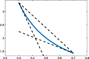
The nonlinearities appearing in power flow are of the form x ² or xy for some variables x,y. We use the following convex envelopes as relaxations of these nonlinear terms:

$$\begin{array}{@{}rcl@{}} \text{SqRel}\left({y,[{{y}}^{L},{{y}}^{U}]}\right)=\left\{x:\begin{array}{l} x \geq y^{2}\\ x \leq \left({{{y}}^{L}+{{y}}^{U}}\right)y-{{y}}^{L}{{y}}^{U} \end{array} \right\} \end{array} $$

(14a)

$$\begin{array}{@{}rcl@{}} \text{McCormick}\left({y,z,[{{y}}^{L},{{y}}^{U}],[{{z}}^{L},{{z}}^{U}]}\right)=\left\{x: \begin{array}{l} x \geq {{y}}^{L}z + {{z}}^{L}y - {{y}}^{L}{{z}}^{L}\\ x \geq {{y}}^{U}z + {{z}}^{U}y - {{y}}^{U}{{z}}^{U}\\ x \leq {{y}}^{L}z - {{z}}^{U}y + {{y}}^{L}{{z}}^{U}\\ x \leq {{z}}^{L}y - {{y}}^{U}z + {{z}}^{L}{{y}}^{U} \end{array} \right\} \end{array} $$

(14b)

1.2 A.2 Interval DP Relaxation

In this section, we describe a concrete implementation of the interval relaxation procedure (13a):

$$\begin{array}{@{}rcl@{}} &&\underset{s_{i},\{S_{k},\mathfrak{v}_{k},\text{Sq}^{P}_{k},,\text{Sq}^{P}_{k},\text{Prod}^{\mathfrak{v},\mathfrak{i}}_{k}\}_{k\in \mathcal{C}\left({i}\right)\cup\{i\}}}{\text{Extremize}} \{\mathfrak{v}_{i},P_{i},Q_{i},a_{i}\left({t}\right)p_{i}+b_{i}\left({t}\right)q_{i}+c_{i}\left({t}\right)\} \end{array} $$

(15a)

$$\begin{array}{@{}rcl@{}} && \text{Subject to} \\ && P_{i} = p_{i}+\sum\limits_{k \in \mathcal{C}\left({i}\right)}\left({P_{k}-\mathfrak{i}_{k}r_{k}}\right) \end{array} $$

(15b)

$$\begin{array}{@{}rcl@{}} && Q_{i} = q_{i}+\sum\limits_{k \in \mathcal{C}\left({i}\right)}\left({Q_{k}-\mathfrak{i}_{k}x_{k}}\right) \end{array} $$

(15c)

$$\begin{array}{@{}rcl@{}} && \mathfrak{v}_{i} = \mathfrak{v}_{k}+\mathfrak{i}_{k}\left({{r_{k}^{2}}+{x_{k}^{2}}}\right)-2\left({P_{k}r_{k}+Q_{k}x_{k}}\right),k \in \mathcal{C}\left({i}\right) \end{array} $$

(15d)

$$\begin{array}{@{}rcl@{}} && \sqrt{{P_{k}^{2}}+{Q_{k}^{2}}} \leq \sqrt{\mathfrak{v}_{k}\mathfrak{i}_{k}}\quad k\in \mathcal{C}\left({i}\right)\cup\{i\} \end{array} $$

(15e)

$$\begin{array}{@{}rcl@{}} && \text{Sq}^{P}_{k}+\text{Sq}^{Q}_{k}=\text{Prod}^{\mathfrak{v},\mathfrak{i}}_{k} \quad k\in \mathcal{C}\left({i}\right)\cup\{i\} \end{array} $$

(15f)

$$\begin{array}{@{}rcl@{}} && \text{Sq}^{P}_{k} \in \text{SqRel}\left({P_{k},P\left({\mathbb{I}_{k}}\right)}\right) \quad k\in \mathcal{C}\left({i}\right)\cup\{i\} \end{array} $$

(15g)

$$\begin{array}{@{}rcl@{}} && \text{Sq}^{Q}_{k} \in \text{SqRel}\left({Q_{k},Q\left({\mathbb{I}_{k}}\right)}\right) \quad k\in \mathcal{C}\left({i}\right)\cup\{i\} \end{array} $$

(15h)

$$\begin{array}{@{}rcl@{}} && \text{Prod}^{\mathfrak{v},\mathfrak{i}}_{k} \in \text{McCormick}\left({\mathfrak{v}_{k},\mathfrak{i}_{k},\mathfrak{v}\left({\mathbb{I}_{k}}\right),\mathfrak{i}\left({\mathbb{I}_{k}}\right)}\right)\quad k\in \mathcal{C}\left({i}\right)\cup\{i\} \end{array} $$

(15i)

$$\begin{array}{@{}rcl@{}} &&\mathfrak{v}_{k} \in \mathfrak{v}\left({\mathbb{I}_{k}}\right), \mathfrak{i}_{k} \in \mathfrak{i}\left({\mathbb{I}_{k}}\right),P_{k}\in P\left({\mathbb{I}_{k}}\right),Q_{k}\in Q\left({\mathbb{I}_{k}}\right),k\in\{i\}\cup\mathcal{C}\left({i}\right) \end{array} $$

(15j)

$$\begin{array}{@{}rcl@{}} && p_{i} \in [{{p_{i}}}^{L}\left({t}\right),{{p_{i}}}^{U}\left({t}\right)],q_{i} \in [{{q_{i}}}^{L}\left({t}\right),{{q_{i}}}^{U}\left({t}\right)] \end{array} $$

(15k)

This requires solution of a small number of SOCPs within each DP update (specifically 10 SOCPs in 6d variables where d is the maximum degree of a node in the tree - note that we can always choose d≤2 by modifying the original problem as in lemma 1). Note also that as the intervals $\mathbb {I}_{k}$ get smaller, the relaxation gets tighter - this is formalized in the lemma below:

Lemma 2

The relaxation defined by ( 15a ) is a valid interval relaxation and satisfies the conditions of the definition 5.

Proof

Through this proof, we use $\eta \left ({M}\right )$ to refer to some constant that depends on the number M from assumption 2. Properties (11a), (10b) are obvious since (15a) is a valid relaxation of the problem (12a). The property (10a) follows from the tightness of the McCormick relaxation. If $\mathbb {I}_{i},\left (\mathbb {I}_{k}\right )_{k\in \mathcal {C}(i)}$ are of radius at most 𝜖, we know that

$${{\mathfrak{v}_{k}}}^{L}\mathfrak{i}_{k}+{{\mathfrak{i}_{k}}}^{L}\mathfrak{v}_{k}-{{\mathfrak{v}_{k}}}^{L}{{\mathfrak{i}_{k}}}^{L} \leq \text{Prod}^{\mathfrak{v},\mathfrak{i}}_{k} \leq {{\mathfrak{v}_{k}}}^{U}\mathfrak{i}_{k}+{{\mathfrak{i}_{k}}}^{L}\mathfrak{v}_{k}-{{\mathfrak{v}_{k}}}^{U}{{\mathfrak{i}_{k}}}^{L}$$

so that the range of $\text {Prod}^{\mathfrak {v},\mathfrak {i}}_{k}$ is of size at most

$$\left({{{\mathfrak{v}_{k}}}^{U}-{{\mathfrak{v}_{k}}}^{L}}\right)\left({\mathfrak{i}_{k}-{{\mathfrak{i}_{k}}}^{L}}\right)\leq \left({{{\mathfrak{v}_{k}}}^{U}-{{\mathfrak{v}_{k}}}^{L}}\right)\left({{{\mathfrak{i}_{k}}}^{U}-{{\mathfrak{i}_{k}}}^{L}}\right)\leq \eta \epsilon$$

since $\mathfrak {i}_{k}$ has upper and lower bounds depending on the problem data. Thus, we know that $\text {Prod}_{k}^{\mathfrak {v},\mathfrak {i}}$ is at most η(M)𝜖 away from $\mathfrak {v}_{k}\mathfrak {i}_{k}$. Similarly, Sq^P _k is at most η(M)𝜖 away from ${P_{k}^{2}}$, Sq^Q _k is at most η(M)𝜖 away from ${Q_{k}^{2}}$. Combining these results, we get the that (10a) holds. □

1.3 A.3 Bound-tightening procedure

We use a scheme similar to the one described in [8] that infers bounds on the variables $\mathfrak {v}_{i},P_{i},Q_{i}, \mathfrak {i}_{i}$ given the constraints in the ACOPF problem (??). Let $\text {Conv}\left ({\mathbf {S}_{i}}\right )$ denote the convex hull of the set S _i . We use a convex relaxation of the constraints (2a) that depends on the variable bounds. We then iterate this procedure where we use a relaxation to infer tighter bounds, and then tighten the relaxation using the inferred bounds. In practice, we find that the procedure converges in a few iterations typically to a stable set of bounds.

The nonconvex constraint ${P_{k}^{2}}+{Q_{k}^{2}}=\mathfrak {v}_{k}\mathfrak {i}_{k}$ can be relaxed to a convex constraint: $\sqrt {{P_{k}^{2}}+{Q_{k}^{2}}}\leq \sqrt {\mathfrak {i}_{k}\mathfrak {v}_{k}}$. This can be tightened by replacing the nonlinear terms in the equation $(P_{k})^{2}+(Q_{k})^{2}=\mathfrak {v}_{k}\mathfrak {i}_{k}$ with their McCormick envelopes. Plugging all this into a single formulation, we obtain:

$$\begin{array}{@{}rcl@{}} \underset{\mathfrak{v},\mathfrak{i},S,s,\text{Sq}^{P},\text{Sq}^{Q},\text{Prod}^{\mathfrak{v},\mathfrak{i}}}{\text{Extremize}} &&\{\mathfrak{v}_{i},\mathfrak{i}_{i},P_{i},Q_{i}\}_{i=1}^{n} \end{array} $$

(16a)

$$\begin{array}{@{}rcl@{}} \text{ Subject to} && S_{i}\,-\,\sum\limits_{k \in \mathcal{C}\left({i}\right)} \left({S_{k}\,-\,\mathfrak{i}_{k}z_{k}}\right) \in \text{Conv}\left({\mathbf{S}_{i}}\right), i \in \{0,\ldots,n\} \end{array} $$

(16b)

$$\begin{array}{@{}rcl@{}} && \mathfrak{v}_{i} \,=\, \mathfrak{v}_{k}+\mathfrak{i}_{k}|z_{k}|^{2}\,-\,2\left({P_{k}r_{k}\,+\,Q_{k}x_{k}}\right), i\in \{0,\ldots,n\}, k \in \mathcal{C}\left({i}\right) \end{array} $$

(16c)

$$\begin{array}{@{}rcl@{}} && \sqrt{{P_{k}^{2}}\,+\,{Q_{k}^{2}}} \leq \sqrt{\mathfrak{v}_{k}\mathfrak{i}_{k}}, k\in \{1,\ldots,n\} \end{array} $$

(16d)

$$\begin{array}{@{}rcl@{}} & &\text{Sq}^{P}_{k}\,+\,\text{Sq}^{Q}_{k}\,=\,\text{Prod}^{\mathfrak{v},\mathfrak{i}}_{k} \quad k\in \{1,\ldots,n\} \end{array} $$

(16e)

$$\begin{array}{@{}rcl@{}} & &\text{Sq}^{P}_{k} \!\in\! \text{SqRel}\left({P_{k},[{{P_{k}}}^{L},{{P_{k}}}^{U}]}\right), k\in \{1,\ldots,n\} \end{array} $$

(16f)

$$\begin{array}{@{}rcl@{}} & &\text{Sq}^{Q}_{k} \!\in\! \text{SqRel}\left({Q_{k},[{{Q_{k}}}^{L},{{Q_{k}}}^{U}]}\right), k\!\in\! \{1,\ldots,n\} \end{array} $$

(16g)

$$\begin{array}{@{}rcl@{}} & &\text{Prod}^{\mathfrak{v},I}_{k} \!\in\! \text{McCormick}\left(\mathfrak{v}_{k},\mathfrak{i}_{k},[{\mathfrak{v}_{k}}^{L},{\mathfrak{v}_{k}}^{U}],[{\mathfrak{i}_{k}}^{L}, {\mathfrak{i}_{k}}^{U}]\right), k\!\in\! \{1,\ldots,n\} \end{array} $$

(16h)

Each minimum/maximum value involves solving a Second Order Cone Program (SOCP) and can be done in parallel over the variables involved. This entire procedure can be viewed as a mapping:

$$\left(\begin{array}{cccccc} {{\mathfrak{v}}}^{L} & {{\mathfrak{v}}}^{U} & {{S}}^{L} & {{S}}^{U} & {{\mathfrak{i}}}^{L} & {{\mathfrak{i}}}^{U} \end{array}\right)_{t} \mapsto \left(\begin{array}{cccccc} {\mathfrak{v}}^{L} & {\mathfrak{v}}^{U} & {\mathfrak{v}}^{L} & {\mathfrak{v}}^{U} & {\mathfrak{i}}^{L} & {\mathfrak{i}}^{U} \end{array}\right)_{t+1}$$

We iterate this mapping until there the improvement in bounds is smaller than some threshold. The obtained bounds are used to redefine the domains $\mathcal {X}_{i}$ for each of the variables.

1.4 A.4 Proof of Lemma 1

We describe a transformation that takes a node i with m children and adds at most $r=\lceil \log _{2}\left ({m}\right )\rceil$ additional buses to create a new network where each node has at most 2 children. We add children in “levels” p=1,…,r: At level 1, we add children c ₁₀,c ₁₁ connected to bus i by 0-impedance transmission lines. We have the following constraints between i and its children ${\mathcal {C}\left ({i}\right )}^{\prime }=\{c_{10},c_{11}\}$:

$$\begin{array}{@{}rcl@{}} S_{i} & =&s_{i}+\sum\limits_{k \in {\mathcal{C}\left({i}\right)}^{\prime}}S_{k} \\ \mathfrak{v}_{i} & =&\mathfrak{v}_{k}, k \in \mathcal{C}\left({i}\right)^{\prime} \\ \mathfrak{i}_{k}\mathfrak{v}_{k} &=& |S_{k}|^{2}, k \in {\mathcal{C}\left({i}\right)}^{\prime} \end{array} $$

At any level p≤r, all nodes are of the form $c_{i_{1}{\ldots } i_{p}}$. We add its children $\mathcal {C}\left ({c_{i_{1}{\ldots } i_{p}}}\right )=\{c_{i_{1}{\ldots } i_{p} 0},c_{i_{1}{\ldots } i_{p} 1}\}$ connected to it by 0-impedance lines with the constraints:

$$\begin{array}{@{}rcl@{}} S_{c_{i_{1}{\ldots} i_{p}}} & =&\sum\limits_{k \in \mathcal{C}\left({c_{i_{1}{\ldots} i_{p}}}\right)}S_{k} \\ \mathfrak{v}_{c_{i_{1}{\ldots} i_{p}}} & =&\mathfrak{v}_{k}, k \in \mathcal{C}\left({c_{i_{1}{\ldots} i_{p}}}\right) \\ \mathfrak{i}_{k}\mathfrak{v}_{k} &=& |S_{k}|^{2}, k \in \mathcal{C}\left({c_{i_{1}{\ldots} i_{p}}}\right) \end{array} $$

At the final level p=r−1, every node is of the form $c_{i_{1}{\ldots } i_{r-1}}$ and its children are picked from the set of original children $\mathcal {C}(i)$. One way of doing this is to assign children in order: $\mathcal {C}\left (c_{10\ldots 0}\right )=\{c_{1},c_{2}\},\mathcal {C}\left ({c_{10{\ldots } 1}}\right )=\{c_{3},c_{4}\},\ldots$. Then, we add the balance equations:

$$\begin{array}{@{}rcl@{}} S_{c_{i_{1}i_{2}{\ldots} i_{r-1}}} & =&\sum\limits_{k \in \mathcal{C}\left({c_{i_{1}i_{2}{\ldots} i_{r-1}}}\right)}\left({S_{k}}\right) \\ \mathfrak{v}_{i} & =&\mathfrak{v}_{k}, k \in \mathcal{C}\left({i}\right)^{\prime} \\ \mathfrak{i}_{k}\mathfrak{v}_{k} &= &|S_{k}|^{2}, k \in {\mathcal{C}\left({i}\right)}^{\prime} \end{array} $$

Adding the power balance equations at all the intermediate buses, we recover the original power balance condition

$$s_{i}=\sum\limits_{k \in \mathcal{C}\left({i}\right)} \left({S_{k}-z_{k}\mathfrak{i}_{k}}\right) $$

Further, we have that $\mathfrak {v}_{i}=\mathfrak {v}_{c_{i_{1}i_{2}{\ldots } i_{p}}}$ for every 1≤p≤r−1.

1.5 A.5 Proof of Theorem 2

Proof

Through this proof, we will use $\zeta \left ({M}\right )$ to denote an arbitrary function of M. The proof of the algorithm breaks down to three key statements:

• 1  The size of the messages |η ⁱ| is bounded by $\frac {\zeta \left ({M}\right )}{\epsilon ^{3}}$.

• 2  For each message, $\text {Rad}\left ({\beta ^{i}\left ({t}\right )}\right )\leq \zeta \left ({M}\right )\epsilon ,t=1\ldots ,|\beta ^{i}|$.

• 3  In the interval DP update Algorithm 2 makes at most $\frac {\zeta \left ({M}\right )}{\epsilon ^{5}}$ calls to the PropBound routine.

Proof of 1,2

For the leaf nodes, the size of the messages is bounded by $|\mathbf {S}_{i}|\left (\frac {{\mathfrak {v}_{i}}^{U}-{\mathfrak {v}_{i}}^{L}}{\epsilon }+1\right )\leq \frac {\zeta \left ({M}\right )}{\epsilon }$ (since ${{\mathfrak {v}}}^{U}_{i}\leq M, {{\mathfrak {v}_{i}}}^{L} \geq \frac {1}{M},|\mathbf {S}_{i}|\leq M$). Since 0<𝜖<1, this is smaller than $\frac {\zeta \left ({M}\right )}{\epsilon ^{3}}$. Further, since ${{p_{i}}}^{U}\left ({t}\right )-p_{i}\left ({t}\right ),{{q_{i}}}^{U}\left ({t}\right )-q_{i}\left ({t}\right )\leq \frac {1}{M}$, we know that $\text {Rad}\left ({\beta ^{i}\left ({t}\right )}\right )\leq \epsilon$ for each t=1,…,|β ⁱ|. For non-leaf node, the size of the messages is bounded by the size of $|\text {Partition}\left (\mathcal {X}_{i},\epsilon \right )|\leq \frac {\zeta (M)}{\epsilon ^{3}}$. Further, since $\beta ^{i}\left ({t}\right ) \subset \mathbb {I}_{i} \in \text {Partition}\left ({\mathcal {X}_{i},\epsilon }\right )$, we know that $\text {Rad}\left ({\beta ^{i}\left ({t}\right )}\right )\leq \epsilon$.

Thus, using (11a), the error of the PF equations $|p_{i}-p_{i}\left ({\beta _{i},\beta _{\mathcal {C}\left ({i}\right )}}\right )|,|q_{i}-q_{i}\left ({\beta _{i},\beta _{\mathcal {C} \left ({i}\right )}}\right )|,|\mathfrak {v}_{i}-\mathfrak {v}_{i}\left ({\beta _{k}}\right )|$ can be bounded by ζ(M)𝜖. This proves claim 1 of the theorem. Further, since at each step we propagate all interval regions consistent with at least one interval value of the child, the optimal solution to the original problem is feasible for the interval relaxation. Thus, for each we have that $c_{i}\left (p_{i}^{\ast },q_{i}^{\ast }\right )\leq c_{i}\left (p_{i}^{OPT},q_{i}^{OPT}\right )$. Adding this over all i gives us claim 2 of the theorem.

Finally, we show that the DP update can be implemented with $\frac {\zeta \left ({M}\right )}{\epsilon ^{5}}$ calls to the PropBound routine. In the loops in algorithm 1, we are implicitly looping over possible interval values of $\mathfrak {v}_{i},P_{i},Q_{i},\mathfrak {v}_{j},P_{j},Q_{j},\mathfrak {v}_{k},P_{k},Q_{k}$. However, these variables are linked by the constraints:

$$\begin{array}{@{}rcl@{}} P_{i} &=&p_{i}+\left({P_{k}-r_{k} \frac{{P_{k}^{2}}+{Q_{k}^{2}}}{\mathfrak{v}_{k}}}\right)+\left({P_{j}-r_{j} \frac{{P_{j}^{2}}+{Q_{j}^{2}}}{\mathfrak{v}_{j}}}\right) \\ Q_{i} & =&q_{i}+\left({Q_{k}-x_{k} \frac{{P_{k}^{2}}+{Q_{k}^{2}}}{\mathfrak{v}_{k}}}\right)+\left({Q_{j}-x_{j} \frac{{P_{j}^{2}}+{Q_{j}^{2}}}{\mathfrak{v}_{j}}}\right) \\ \mathfrak{v}_{i} & =&\mathfrak{v}_{k}+\left({r_{k}^{2}}+{x_{k}^{2}}\right)\frac{\left({P_{k}^{2}}+{Q_{k}^{2}}\right)}{\mathfrak{v}_{k}}-2\left(P_{k}r_{k}+Q_{k}x_{k}\right) \\ \mathfrak{v}_{i} & =&\mathfrak{v}_{j}+\left({r_{j}^{2}}+{x_{j}^{2}}\right)\frac{\left({P_{j}^{2}}+{Q_{j}^{2}}\right)}{\mathfrak{v}_{j}}-2\left(P_{j}r_{j}+Q_{j}x_{j}\right) \end{array} $$

Thus, if p _i ,q _i are fixed, the 9 variables are constrained to lie on a 5-dimensional manifold (since there are 4 non-redundant . This suggests that we only need to do an exhaustive search over a 5-dimensional space rather than a 9 dimensional space.

Suppose $p_{i}\in [{{p_{i}}}^{L}\left ({t}\right ),{{p_{i}}}^{U}\left ({t}\right )],q_{i}\in [{q_{i}}^{L}(t), {q_{i}}^{U}(t)]$ and we fix particular interval values (of radius smaller than 𝜖) for variables $\mathfrak {v}_{i},P_{k},Q_{k},P_{j},Q_{j}$. Then, from the first two equations, we know that P _i ,Q _i must lie in an interval of size ζ(M)𝜖 (since p _i ,q _i lie in intervals of size $\zeta \left ({M}\right )$). Thus, we need to loop over at most $\zeta \left ({M}\right )$ possible values of P _i ,Q _i . Similarly, if $\mathfrak {v}_{i},P_{k},Q_{k}$ are fixed to interval values of radius 𝜖, the third equation says that $\mathfrak {v}_{k}$ must lie in an interval of size $\zeta \left ({M}\right )\epsilon$, and similarly if $\mathfrak {v}_{i},P_{j},Q_{j}$ are fixed to intervals of radius of 𝜖, $\mathfrak {v}_{j}$ must lie in an interval of size $\zeta \left ({M}\right )\epsilon$. Thus, we need to loop over at most $\zeta \left ({M}\right )$ possible values of $\mathfrak {v}_{j},\mathfrak {v}_{k},P_{i},Q_{i}$ once the values of $\mathfrak {v}_{i},P_{k},Q_{k},P_{j},Q_{j}$ are fixed to intervals of radius 𝜖. Finally, the total number of loops in algorithm 2 is at most $\frac {\zeta (M)}{\epsilon ^{5}}$. Adding this over all nodes of the network, we get the third claim of Theorem 2. □

References

Achterberg, T. (2009). SCIP: solving constraint integer programs. Mathematical Programming Computation, 1(1), 1–41.
Baran, M. E., & Wu, F. F. (1989). Optimal capacitor placement on radial distribution systems. IEEE Transactions on Power Delivery, 4(1), 725–734.
Bienstock, D., & Munoz, G. (2015). LP approximations to mixed-integer polynomial optimization problems ArXiv e-prints.
Bienstock, D., & Verma, A. (2015). Strong NP-hardness of AC power flows feasibility. arXiv:http://arXiv.org/abs/1512.07315.
Bonami, P., Biegler, L. T., Conn, A. R., Cornuéjols, G., Grossmann, I. E., Laird, C. D., & Lee, J., Lodi, A., Margot, F., Sawaya, N., et al. (2008). An algorithmic framework for convex mixed integer nonlinear programs. Discrete Optimization, 5(2), 186–204.
Bose, S., Gayme, D., Chandy, K., & Low, S. (2015). Quadratically constrained quadratic programs on acyclic graphs with application to power flow. IEEE Transactions on Control of Network Systems, 2(3), 278–287. doi:http://dx.doi.org/10.1109/TCNS.2015.2401172.
Carpentier, J. (1962). Contribution to the economic dispatch problem. Bulletin de la Société Française des Electriciens, 3(8), 431–447.
Coffrin, C., Hijazi, H. L., & Van Hentenryck, P. (2015). Strengthening convex relaxations with bound tightening for power network optimization. In Principles and Practice of Constraint Programming (pp. 39–57): Springer.
Dechter, R. (2003). Constraint processing.
Dunning, I., Huchette, J., & Lubin, M. (2015). JuMP: A modeling language for mathematical optimization. arXiv:1508.01982 [math.OC].
Gamarnik, D., Shah, D., & Wei, Y. (2012). Belief propagation for min-cost network flow: Convergence and correctness. Operations Research, 60(2), 410–428.
Gan, L., Li, N., Topcu, U., & Low, S. H. (2015). Exact convex relaxation of optimal power flow in radial networks. IEEE Transactions on Automatic Control, 60 (1), 72–87.
Johnson, J. K. (2008). Convex relaxation methods for graphical models: Lagrangian and maximum entropy approaches. Ph.D. thesis Massachusetts Institute of Technology.
Kakade, S. M., Kearns, M., & Ortiz, L. E. (2004). Graphical economics. In International Conference on Computational Learning Theory (pp. 17–32): Springer.
Kearns, M., Littman, M. L., & Singh, S. (2001). Graphical models for game theory. In Proceedings of the Seventeenth Conference on Uncertainty in Artificial Intelligence (pp. 253–260): Morgan Kaufmann Publishers Inc.
Koller, D., & Friedman, N. (2009). Probabilistic graphical models: principles and techniques: MIT Press.
Kschischang, F. R., Frey, B. J., & Loeliger, H. A. (2001). Factor graphs and the sum-product algorithm. IEEE Transactions on Information Theory, 47(2), 498–519.
Lavaei, J., Tse, D., & Zhang, B. (2013). Geometry of power flows and optimization in distribution networks.
Lehmann, K., Grastien, A., & Van Hentenryck, P. (2016). AC-feasibility on tree networks is NP-hard. IEEE Transactions on Power Systems, 31(1), 798–801. doi:10.1109/TPWRS.2015.2407363.
Low, S. H. (2014). Convex relaxation of optimal power flow, part i: Formulations and equivalence. arXiv preprint arXiv:1405.0766.
Low, S. H. (2014). Convex Relaxation of Optimal Power Flow, Part II: Exactness. ArXiv eprints.
Ortiz, L. E. (2014). On sparse discretization for graphical games. arXiv:1411.3320.
Ortiz, L. E., & Irfan, M. T. (2016). FPTAS for mixed-strategy nash equilibria in tree graphical games and their generalizations. arXiv:1602.05237.
Pai, M., & Chatterjee, D. (2014). Computer techniques in power system analysis. India: McGraw-Hill Education.
Sojoudi, S., & Lavaei, J. (2014). Exactness of semidefinite relaxations for nonlinear optimization problems with underlying graph structure. SIAM Journal on Optimization, 24(4), 1746–1778.
Sontag, D. A. (2010). Approximate inference in graphical models using LP relaxations: Ph.D. thesis Massachusetts Institute of Technology.
Vigerske, S., & Gleixner, A. (2016). SCIP: Global optimization of mixed-integer nonlinear programs in a branch-and-cut framework.
Vittal, V., & Bergen, A. R. (1999). Power systems analysis: Prentice Hall.
Wainwright, M. J., & Jordan, M. I. (2008). Graphical models, exponential families, and variational inference. Foundations and Trends \({\circledR }\) in Machine Learning, 1(1-2), 1–305.
Author information
Authors and Affiliations
Corresponding author
Additional information
This work was supported by Skoltech through collaboration agreement 1075-MRA. The work at LANL was carried out under the auspices of the National Nuclear Security Administration of the U.S. Department of Energy under Contract No. DE-AC52-06NA25396.