Systematic simulations of FFP scattering by a star–planet pair

Abstract

The increasing number of free-floating planets discovered in recent years confirms earlier theoretical predictions and leads us to believe that the possibility of such an object intruding an existing planetary system is not negligible, especially in dense clusters. We present a theoretical dynamical study on the interaction of a free-floating planet (hereafter FFP) with an initially bound star–planet pair consisting of a Jupiter-sized planet (hereafter BP) orbiting a Sun-like star. Our results could serve as a base for analytical, or semi-analytical, studies on the three-dimensional three-body scattering problem. In our three-dimensional models, thousands of different trajectories for an incoming FFP with initially parabolic velocity are integrated, in order to investigate the interaction between the objects. The study is based on two independent approaches, in order to corroborate the significance of the results. In the first approach, the FFP interacts with a Solar-like system (hereafter SlS) consisting of the Sun and Jupiter at $5.2\,\mathrm{AU}$. In the second, we compute the trajectories of a FFP interacting with a closely bound exoplanetary system (hereafter ES) with the Jupiter-sized planet at an orbit of $1\,\mathrm{AU}$ around its host, Sun-like star. For both approaches, the simulations have five free parameters, namely the initial phase of the BP, $\phi _{BP}$, the mass, $m_{FFP}$, the initial inclination, $i_{FFP}$, the orientation of the velocity vector of the FFP and the impact parameter $d_{FFP}=d$. We focus on three possible final states, namely “flyby,” “capture” and “exchange.” One can observe that the overall picture does not change between the two models used. We present a statistical analysis of the data and the probabilities for the different outcomes for both. Capture and flyby are dominant, in almost equal parts, while the probability for an exchange is rather low. A close look of the orbital elements in case of a capture of the FFP provides more information on the dynamical behavior of the two models, allowing us to draw more precise conclusions, when it comes to the similarities and differences between them. Different mass, as well as different orientation of the velocity vector of the incoming planet, does affect the final outcome quantitatively and qualitatively, in both cases.

Appendices

Exoplanetary system—ES

According to—biased¹³—observations of exoplanetary systems,¹⁴ the Jupiter–mass BP is initially set on an orbit close to the star with $r_0= 1$ AU.

The initial values of the inclination for the trajectory of the FFP are varied from $0^{\circ }$ to $45^{\circ }$. Any inclination above $45^{\circ }$ is not taken into account due to the fact that for these high initial inclinations the total distance from the star–planet pair increases substantially, a fact that affects the velocity reached when encountering the system. This would make the comparison with the SlS model, where the total distance from the star is a fixed value, more difficult. This setup is illustrated in Fig. 26.

x-, y- and z-values have the unit $\,\mathrm{AU}$ for the ES case, while the velocities of the objects are given in AU / days.

Fig. 26

ES: initial positions of the three bodies: the Sun-like star is placed at the origin, the bound Jupiter-sized planet is initially on a circular orbit with $r_{0} = 1$ AU around the star and the incoming FFP is started from a fixed x-distance of $x_{0}$ = 40 AU with a parabolic velocity. The initial state of the system is determined by the initial phase $\phi _{BP}$ of the BP and the y-and z-position of the FFP. In this work, the y-position of the FFP is referred to as impact parameter d of the incoming planet

With the x-position of the FFP fixed to 40, the other initial conditions are the following: The starting point of the BP is changed by varying the initial phase of the BP from $0^{\circ } \le \phi \le 360^{\circ }$. Therefore, the initial coordinates of the BP in the ES case are calculated as follows:

• $x=r_{0} \cos (\phi _{BP}) ; \, y=r_0 \sin (\phi _{BP}); \, z=0$

• ${\dot{x}}=-k \sin (\phi _{BP}); \, {\dot{y}}= k \cos (\phi _{BP}) \,\, \mathrm {and} \,\, {\dot{z}}=0$,

with $\phi _{BP}$ being the initial phase of the BP and k, the Gaussian gravitational constant. The incoming FFP holds the following initial conditions:

• $x = -40r_{0} ; \, y=d; \, z=\tan (i_{FFP}) \cdot x$

• ${\dot{x}} = v \cos (i_{FFP}); \, {\dot{y}}=0 \,\, \mathrm {and} \,\, {\dot{z}}= -v \sin (i_{FFP})$.

The FFP is started on a trajectory parallel to the projected x-axis in a plane that is inclined with the value $i_{FFP}$ to the xy-plane. The initial velocity v of the FFP is calculated through Eq. 1 for each initial position of the FFP.

In total, the ES scenario contains

• 360 initial positions for the BP ($\phi _{BP}$ from $0^{\circ }$ to $360^{\circ }$ with $\Delta \phi _{BP}=1^{\circ }$)

• 140 initial y-positions for the FFP ($-7 \le d \le 7$ with $\Delta d=0.1 AU$)

• 180 initial z-positions for the FFP ($0^{\circ }$ to $45^{\circ }$ with $\Delta i=0.25^{\circ }$),

which gives a total of 9,072,000 initial conditions.

Solar system—SS

The initial conditions for the BP and the star are the same as in the ES case (see Chapter A). The system of units where $G=M_{star}=M_{\odot }=r_{0}=1$ places the BP at a distance of $\mathbf {r_{0}}$, with an initial velocity $\mathbf {v_{0}}$ that corresponds to a circular orbit around the star, with $T=2\pi$ and $|\mathbf {v_{0}}|=1$.

In contrast to the ES, where the x-distance of the FFP to the center of mass is fixed, in the SlS scenario the FFP is coming from a fixed total distance (“infinity”), equal to $|\mathbf {r}|=|40\mathbf {r_{0}}|$, with a parabolic velocity $|\mathbf {v}|$ with respect to the star (see Sect. 2.2).

Fig. 27

Isolated grid of initial positions with $0<x<40r_{0}$, $-7r_{0}<y<7r_{0}$, $0<z<40r_{0}$. The RGB lines correspond to the triorthogonal xyz axes system, respectively

Fig. 28

Computation of w angle: in this setup $0^{\circ }\le w\le 20^{\circ }$. If we combine this angle and the coordinates of the velocity vector, we derive $\omega$, the angle that provides the orientation of the velocity vector on the xz-plane: $170^{\circ }+\theta {'}<\omega <190^{\circ }+\theta {'}$. We must note that $\theta =\theta {'}$ only when $\phi =0^{\circ }$

Because of the symmetry, we need only one hemisphere in the SlS scenario, which we choose to be the “above” (positive values of z). Taking advantage of the motion of the BP, we can further restrict ourselves, to only one quarter of the sphere, i.e., $x,(-y,y),z$ (see Fig. 27).

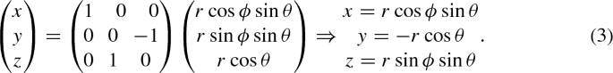
The classical formulation of spherical coordinates does not provide the constant surface density on the region of the grid of initial positions of the FFP we will use, which is a necessity in order to proceed. We use the rotation matrix $Z_{1}X_{2}Z_{3}$, to ensure that both the star–BP and the star–FFP system are counterclockwise¹⁵.

In the SlS case, each initial position on the grid defines a plane parallel to the xz-plane. The initial velocity vector of the FFP at each point will be split into two components $v_{x}$, $v_{z}$ with $v_{y}=0$. We are able to initially use only these two components, by taking advantage of the circular motion of the BP around the star. The “impact parameter” (in the remaining two dimensions) for the velocity vector will here be defined by the radius R, $0\le {R}\le {7r_{0}}$, of the circle with center at $(0,[-y,y],0)$ on each plane. The range of R corresponds to an angle w of the velocity vector of range $0^{\circ }\le w\le 20^{\circ }$ (Fig. 28). With the help of some imagination, the locus of the “impact parameter” is a set of homocentric cylinders (side surface) with axes that coincide with the y-axis of the system. The $\omega$ angle is used to set the direction of the velocity vector toward a circular section of the cylinder (orientation), of range $170^{\circ }+\theta {'}<\omega <190^{\circ }+\theta {'}$ (Fig. 28), with:

$$\begin{aligned} \sin (90^{\circ }-\theta {'})=\frac{\sin (90^{\circ }-\theta )}{\sqrt{\sin ^{2}(90^{\circ }-\theta )+\cos ^{2}(90^{\circ }-\theta )\cos ^{2}\phi }}, \end{aligned}$$

(4)

where $\theta$ is the polar angle and $\phi$ the azimuthal angle of each initial position.

Finally, the total number of initial conditions for one value of the mass of the FFP is:

• 29241 initial positions of the FFP (grid). The range of the phase angle, $\phi _{FFP}$, is $\sim -10^{\circ }-\sim 10^{\circ }$, and the range of the azimuthal angle, $\theta$, is $0^{\circ }-90^{\circ }$ which corresponds to the interval set for the projection of the impact parameter on the y-axis. This number of initial positions is obtained for a step of $0.25^{\circ }$ for both angles.

• 21 velocity vectors for the FFP for each initial position with w (angle of the velocity vector) in $0^{\circ } \le \omega \le 20^{\circ }$ and $\Delta \omega$ = $1^{\circ }$. To make it easier to reference, we use the notation v1-v21, for each one of the velocity vectors, with v1 being close to the lower limit, $\omega = 0^{\circ }$ (i.e. $170^{\circ } + \theta ')$ v2 corresponds to $\omega = 1^{\circ }(170^{\circ } + (20^{\circ } = \theta '))$, and a “special case”-v11 pointing at the center of the reference frame (0,0,0) with $\omega = 10^{\circ }$ (Fig. 28).

• 180 initial positions for the BP $0^{\circ }\le \phi _{BP} \le 360^{\circ }$ with $\Delta \phi _{BP}$ = $2^{\circ }$.

Therefore we integrated $29241\times 21\times 180=\mathbf {110,530,980}$ orbits in all, sufficient enough to extract safe statistical results.

References

Bihain, G., Rebolo, R., Zapatero, O.M., Bejar, V.J.S.R., Villo-Perez, I., Diaz-Sanchez, A., et al.: Candidate free-floating super-Jupiters in the young \(\sigma \) Orionis open cluster. A&A 506, 1169–1182 (2009)
Bleher, S., Grebogi, C., Ott, E.: Bifurcation to chaotic scattering. Physica D Nonlinear Phenom. 46, 87 (1990)
Donnison, J.R.: The stability of masses during three-body encounters. Celest. Mech. 32, 145–162 (1984a)
Donnison, J.R.: The stability of planetary star systems during encounters with a third star. Mon. Not. R. Astron. Soc. 210, 915–927 (1984b)
Donnison, J.R.: The Hill stability of a binary or planetary system during encounters with a third inclined body. Mon. Not. R. Astron. Soc. 369, 1267–1280 (2006)
Donnison, J.R.: The Hill stability of a binary or planetary system during encounters with a third inclined body moving on a hyperbolic orbit. Planet. Space Sci. 56, 927–940 (2008)
Donnison, J.R.: The Hill stability of inclined bound triple star and planetary systems. Planet. Space Sci. 57, 771–783 (2009)
Donnison, J.R.: The Hill stability of inclined small mass binary systems in three-body systems with special application to triple star systems, extrasolar planetary systems and Binary Kuiper Belt systems. Planet. Space Sci. 58, 1169–1179 (2010)
Durand-Manterola, H.J.: Free-floating planets: a viable option for panspermia (2010)
Fogg, M.J.: Interstellar planets. Comments Astrophys. 14(6), 357–375 (1990)
Fogg, M.J.: Free-floating planets: their origin and distribution. M.Sc. Astrophysics Project, August 2002. University of London, Queen Mary College (2002)
Hadjidemetriou, J.D.: Binary systems with decreasing mass, 1966b. Z. Astrophys. 63, 116 (1966)
Hairer, E., Wanner, G.: Solving ordinary differential equations II. Stiff and differential—algebraic problems., Springer Series in Computational Mathematics, vol 14, 2nd edn. Springer 1991 (1996)
Han, C., Chung, S.J., Kim, D., Park, B.G., Ryu, Y.H., Kang, S., et al.: Gravitational microlensing: a tool for detecting and characterizing free-floating planets. Astrophys. J 604, 372–378 (2004)
Han, C.: Secure Identifcation of free-floating planets. Astrophys. J 644, 1232–1236 (2006)
Hanslmeier, A., Dvorak, R.: Numerical integration with Lie series. Astron. Astrophys. 132, 203 (1984)
Hoyle, F.: On the fragmentation of gas clouds into galaxies and stars. Astorophys J. 118.513H (1953)
Hurley, J.R., Shara, M.M.: Free-floating planets in stellar clusters: not so surprising. Astrophys. J. 565, 1251–1256 (2002)
Kroupa, P., Bouvier, J.: On the origin of brown dwarfs and free-floating planetary-mass objects. MNRAS 346, 369–380 (2003)
Larson, R.B.: The evolution of protostars-theory. Fundam. Cosmic Phys. 1, 1–70 (1973)
Lissauer, J.J.: Urey prize lecture: on the diversity of plausible planetary systems. Icarus 114, 217–236 (1995)
Low, C., Lynden-Bell, D.: The minimum Jeans mass or when fragmentation must stop. MNRAS 176, 367–390 (1976)
Marchal C.: The three-body problem. ISBN:0-444-87440-2(vol. 4) (1990)
Mroz P. et al.: No large population of unbound or wide-orbit Jupiter-mass planets, astro-ph.EP, 24 Jul (2017)
Padoan, P., Nordlund, A.: The stellar initial mass function from turbulent fragmentation. Astrophys. J 576(2), 870–879 (2002)
Padoan, P., Nordlund, A.: The “mysterious” origin of brown dwarfs. Astrophys. J 617(1), 559–564 (2004)
Padoan, P., et al.: Two regimes of turbulent fragmentation and the stellar initial mass function from primordial to present-day star formation. Astrophys. J. 661, 972–981 (2007)
Quanz, S.P., et al.: Direct imaging constraints on planet populations detected by microlensing. A&A 541, A133 (2012)
Rees, M.J.: Opacity-limited hierarchical fragmentation and the masses of protostars. MNRAS 176, 483–486 (1976)
Silk, J.: On the fragmentation of cosmic gas clouds. II-Opacity-limited star formation. Astrophys. J Part 1 1(214), 152–160 (1977)
Varvoglis, H., Sgardeli, V., Tsiganis, K.: Interaction of free-floating planets with a star-planet pair. Celest. Mech. Dyn. Astron. 113, 387–40 (2012)
Smith, K.W., Bonnell, I.A.: Free-floating planets in stellar clusters? Mon. Not. R. Astron. Soc. 322, L1–L4 (2001)
Sumi, T., Kamiya, K., Bennett, D.P., et al.: Unbound or distant planetary mass population detected by gravitational microlensing. Nature 473, 349 (2011)
Veras, D., et al.: The great escape: how exoplanets and smaller bodies desert dying stars. Mon. Not. R. Astron. Soc. 417, 2104–2123 (2011)
Whitworth, A.P., Goodwin, S.P.: The formation of brown dwarfs. Astron. Nachr. AN 326(10), 899–904 (2005)
Whitworth, A.P., Stamatellos, D.: The minimum mass for star formation, and the origin of binary brown dwarfs. A&A. 458, 817–829 (2006)
Whitworth, A.P., Zinnecker, H.: The formation offree-floating brown dwarves and planetary-mass objects by photo-erosion of prestellar cores. A&A. 427, 299–306 (2004)
Zapatero, O., et al.: Discovery of young, isolated planetary mass objects in the sigma Orionis star cluster. Science 290, 103–107 (2000)
Zapatero Osorio, M.R., Bejar, V.J.S., Pena Ramirez, K.: Optical and near-infrared spectroscopy of free-floating planets in the sigma Orionis cluster. Mem. Soc. Astron. Ital. 84, 926 (2013)
Zapatero Osorio, M.R., Galvez Ortiz, M.C., Bihain, G., Bailer-Jones, C.A.L., Rebolo, R., Henning, T., et al.: Search for free-floating planetary-mass objects in the Pleiades. A&A 568, 77 (2014)
Zinnecker, H.: A free-floating planet population in the Galaxy? ASP Conf. Ser. 239, 2000 (2000)
Acknowledgements
B. Loibnegger acknowledges support by the Austrian Science Fund (FWF) through grant S11603-N16. V. Doultsinou would like to thank the HellasGRID AUTh team for the extra sources and technical support.
Author information
Authors and Affiliations
Corresponding author
Ethics declarations
Conflict of Interest
The authors declare that they have no conflict of interest.
Additional information
Publisher's Note
Springer Nature remains neutral with regard to jurisdictional claims in published maps and institutional affiliations.