On the Sample Complexity of the Linear Quadratic Regulator

Abstract

This paper addresses the optimal control problem known as the linear quadratic regulator in the case when the dynamics are unknown. We propose a multistage procedure, called Coarse-ID control, that estimates a model from a few experimental trials, estimates the error in that model with respect to the truth, and then designs a controller using both the model and uncertainty estimate. Our technique uses contemporary tools from random matrix theory to bound the error in the estimation procedure. We also employ a recently developed approach to control synthesis called System Level Synthesis that enables robust control design by solving a quasi-convex optimization problem. We provide end-to-end bounds on the relative error in control cost that are optimal in the number of parameters and that highlight salient properties of the system to be controlled such as closed-loop sensitivity and optimal control magnitude. We show experimentally that the Coarse-ID approach enables efficient computation of a stabilizing controller in regimes where simple control schemes that do not take the model uncertainty into account fail to stabilize the true system.

Appendices

Proof of Lemma 1

First, recall Bernstein’s lemma. Let $X_1, \ldots , X_p$ be zero-mean independent r.v.s satisfying the Orlicz norm bound $||X_i ||_{\psi _1} \le K$. Then as long as $p \ge 2 \log (1/\delta )$, with probability at least $1-\delta$,

$$\begin{aligned} \sum _{i=1}^{p} X_i \le K \sqrt{2n \log (1/\delta )} \,. \end{aligned}$$

Next, let Q be an $m \times n$ matrix. Let $u_1, \ldots , u_{M_\varepsilon }$ be a $\varepsilon$-net for the m-dimensional $\ell _2$ ball, and similarly let $v_1,\ldots , v_{N_\varepsilon }$ be a $\varepsilon$ covering for the n-dimensional $\ell _2$ ball. For each $||u ||_2=1$ and $||v ||_2=1$, let $u_i$, $v_j$ denote the elements in the respective nets such that $||u - u_i ||_2 \le \varepsilon$ and $||v - v_j ||_2 \le \varepsilon$. Then,

$$\begin{aligned} u^*Q v&= (u - u_i + u_i)^*Q v = (u - u_i)^*Q v + u_i^*Q ( v - v_j + v_j ) \\&= (u - u_i)^*Q v + u_i^*Q ( v - v_j ) + u_i^*Q v_j \,. \end{aligned}$$

Hence,

$$\begin{aligned} u^*Q v \le 2 \varepsilon ||Q ||_2 + u_i^*Q v_j \le 2 \varepsilon ||Q ||_2 +\max _{1 \le i \le M_\varepsilon , 1 \le j \le N_\varepsilon } u_i^*Q v_j \,. \end{aligned}$$

Since u, v are arbitrary on the sphere,

$$\begin{aligned} ||Q ||_2 \le \frac{1}{1-2\varepsilon } \max _{1 \le i \le M_\varepsilon , 1 \le j \le N_\varepsilon } u_i^*Q v_j \,. \end{aligned}$$

Now we study the problem at hand. Choose $\varepsilon = 1/4$. By a standard volume comparison argument, we have that $M_\varepsilon \le 9^m$ and $N_\varepsilon \le 9^n$, and that

$$\begin{aligned} \left\| \sum _{k=1}^{N} f_k g_k^* \right\| _2 \le 2 \max _{1 \le i \le M_\varepsilon , 1 \le j \le N_\varepsilon } \sum _{k=1}^{N} (u_i^*f_k) (g_k^*v_j) \,. \end{aligned}$$

Note that $u_i^*f_k \sim N(0, u_i^*\Sigma _f u_i)$ and $g_k^*v_j \sim N(0, v_j^*\Sigma _g v_j)$. By independence of $f_k$ and $g_k$, $(u_i^*f_k)(g_k^*v_j)$ is a zero mean sub-exponential random variable, and therefore, $||(u_i^*f_k)(g_k^*v_j) ||_{\psi _1} \le \sqrt{2} ||\Sigma _f ||_2^{1/2} ||\Sigma _g ||_2^{1/2}$. Hence, for each pair $u_i, v_j$ we have with probability at least $1 - \delta /9^{m+n}$,

$$\begin{aligned} \sum _{k=1}^{N} (u_i^*f_k) (g_k^*v_j) \le 2||\Sigma _f ||_2^{1/2}||\Sigma _g ||_2^{1/2} \sqrt{N (m + n) \log (9/\delta )} \,. \end{aligned}$$

Taking a union bound over all pairs in the $\varepsilon$-net yields the claim.

Proof of Proposition 3

For this proof, we need a lemma similar to Lemma 1. The following is a standard result in high-dimensional statistics [58], and we state it here without proof.

Lemma 7

Let $W \in {\mathbb {R}}^{N \times n}$ be a matrix with each entry i.i.d. ${\mathcal {N}}(0, \sigma _w^2)$. Then, with probability $1 - \delta$, we have

$$\begin{aligned} \Vert W\Vert _2 \le \sigma _w(\sqrt{N} + \sqrt{n} + \sqrt{2 \log (1/\delta )}). \end{aligned}$$

As before we use Z to denote the $N \times (n+ p)$ matrix with rows equal to $z_\ell ^\top = \begin{bmatrix} (x^{(\ell )})^\top&(u^{(\ell )})^\top \end{bmatrix}$. Also, we denote by W the $N \times n$ matrix with columns equal to $w^{(\ell )}$. Therefore, the error matrix for the ordinary least squares estimator satisfies

$$\begin{aligned} E = \begin{bmatrix} ({\widehat{A}}- A)^\top \\ ({\widehat{B}}- B)^\top \end{bmatrix} = (Z^\top Z)^{-1} Z^\top W, \end{aligned}$$

when the matrix Z has rank $n+ p$. Under the assumption that $N \ge n+ p$ we consider the singular value decomposition $Z = U \Lambda V^\top$, where $V, \Lambda \in {\mathbb {R}}^{(n+ p) \times (n+ p) }$ and $U \in {\mathbb {R}}^{N \times (n+ p)}$. Therefore, when $\Lambda$ is invertible,

$$\begin{aligned} E = V (\Lambda ^\top \Lambda )^{-1} \Lambda ^\top U^\top W = V \Lambda ^{-1} U^\top W. \end{aligned}$$

This implies that

$$\begin{aligned} E E^\top&= V \Lambda ^{-1} U^\top W W^\top U \Lambda ^{-1} V^\top \preceq \Vert U^\top W\Vert _2^2 V \Lambda ^{-2} V^\top = \Vert U^\top W\Vert _2^2 (Z^\top Z)^{-1}. \end{aligned}$$

Since the columns of U are orthonormal, it follows that the entries of $U^\top W$ are i.i.d. ${\mathcal {N}}(0, \sigma _w^2)$. Hence, the conclusion follows by Lemma 7.

Derivation of the LQR Cost as an ${\mathcal {H}}_2$ Norm

In this section, we consider the transfer function description of the infinite horizon LQR optimal control problem. In particular, we show how it can be recast as an equivalent ${\mathcal {H}}_2$ optimal control problem in terms of the system response variables defined in Theorem 1.

Recall that stable and achievable system responses $({\varvec{\Phi }}_x,{\varvec{\Phi }}_u)$, as characterized in Eq. (23), describe the closed-loop map from disturbance signal $\mathbf {w}$ to the state and control action $(\mathbf {x}, \mathbf {u})$ achieved by the controller $\mathbf {K} = {\varvec{\Phi }}_u {\varvec{\Phi }}_x^{-1}$, i.e.,

$$\begin{aligned} \begin{bmatrix} \mathbf {x} \\ \mathbf {u} \end{bmatrix} = \begin{bmatrix} {\varvec{\Phi }}_x \\ {\varvec{\Phi }}_u \end{bmatrix} \mathbf {w}. \end{aligned}$$

Letting ${\varvec{\Phi }}_x = \sum _{t=1}^\infty \Phi _x(t) z^{-t}$ and ${\varvec{\Phi }}_u = \sum _{t=1}^\infty \Phi _u(t) z^{-t}$, we can then equivalently write for any $t \ge 1$

$$\begin{aligned} \begin{bmatrix} x_t \\ u_t \end{bmatrix} = \sum _{k=1}^t\begin{bmatrix} \Phi _x(k) \\ \Phi _u(k) \end{bmatrix} w_{t-k}. \end{aligned}$$

(47)

For a disturbance process distributed as $w_t {\mathop {\sim }\limits ^{{{\mathrm{i.i.d.}}}}}{\mathcal {N}}(0,\sigma _w^2 I_n)$, it follows from Eq. (47) that

$$\begin{aligned} {\mathbb {E}}\left[ x_t^*Q x_t\right]&= \sigma _w^2\sum _{k=1}^t {{\,\mathrm{{{\mathbf {T}}}{{\mathbf {r}}}}\,}}(\Phi _x(k)^*Q\Phi _x(k)) \,, \\ {\mathbb {E}}\left[ u_t^*R u_t\right]&= \sigma _w^2\sum _{k=1}^t {{\,\mathrm{{{\mathbf {T}}}{{\mathbf {r}}}}\,}}(\Phi _u(k)^*R\Phi _u(k)) \,. \end{aligned}$$

We can then write

$$\begin{aligned} \lim _{T\rightarrow \infty } \frac{1}{T} \sum _{t=1}^T {\mathbb {E}}\left[ x_t^*Q x_t + u_t^*R u_t\right]&= \sigma _w^2\left[ \sum _{t=1}^\infty {{\,\mathrm{{{\mathbf {T}}}{{\mathbf {r}}}}\,}}(\Phi _x(t)^*Q\Phi _x(t)) + {{\,\mathrm{{{\mathbf {T}}}{{\mathbf {r}}}}\,}}(\Phi _u(t)^*R\Phi _u(t))\right] \\&= \sigma _w^2\sum _{t=1}^\infty \left\| \begin{bmatrix} Q^\frac{1}{2}&0 \\ 0&R^\frac{1}{2} \end{bmatrix}\begin{bmatrix} \Phi _x(t) \\ \Phi _u(t) \end{bmatrix} \right\| _F^2 \\&= \frac{\sigma _w^2}{2\pi } \int _{{\mathbb {T}}} \left\| \begin{bmatrix} Q^\frac{1}{2}&0 \\ 0&R^\frac{1}{2} \end{bmatrix}\begin{bmatrix} {\varvec{\Phi }}_x \\ {\varvec{\Phi }}_u \end{bmatrix} \right\| _F^2 \; dz \\&=\sigma _w^2 \left\| \begin{bmatrix} Q^\frac{1}{2}&0 \\ 0&R^\frac{1}{2} \end{bmatrix}\begin{bmatrix} {\varvec{\Phi }}_x \\ {\varvec{\Phi }}_u \end{bmatrix} \right\| _{{\mathcal {H}}_2}^2 \,, \end{aligned}$$

where the second to last equality is due to Parseval’s theorem.

Proof of Theorem 4

To understand the effect of restricting the optimization to FIR transfer functions, we need to understand the decay of the transfer functions ${\mathfrak {R}}_{{\widehat{A}}+{\widehat{B}}K_\star }$ and $K_\star {\mathfrak {R}}_{{\widehat{A}}+{\widehat{B}}K_\star }$. To this end, we consider $C_\star > 0$ and $\rho _\star \in (0, 1)$ such that $\Vert (A+ BK_\star )^t \Vert _2 \le C_\star \rho _\star ^t$ for all $t \ge 0$. Such $C_\star$ and $\rho _\star$ exist because $K_\star$ stabilizes the system $(A, B)$. The next lemma quantifies how well $K_\star$ stabilizes the system $({\widehat{A}}, {\widehat{B}})$ when the estimation error is small.

Lemma 8

Suppose $\epsilon _A + \epsilon _B \Vert K_\star \Vert _2 \le \frac{1 - \rho _\star }{2 C_\star }$. Then,

$$\begin{aligned} \Vert ({\widehat{A}}+ {\widehat{B}}K_\star )^t \Vert _2 \le C_\star \left( \frac{1 + \rho _\star }{2} \right) ^t \; \text {, for all } \; t \ge 0. \end{aligned}$$

Proof

The claim is obvious when $t = 0$. Fix an integer $t \ge 1$ and denote $M = A+ BK_\star$. Then, if $\Delta = \Delta _A + \Delta _B K_\star$, we have ${\widehat{A}}+ {\widehat{B}}K_\star = M + \Delta$.

Consider the expansion of $(M+\Delta )^t$ into $2^t$ terms. Label all these terms as $T_{i,j}$ for $i=0,\ldots , t$ and $j=1,\ldots , {t \atopwithdelims ()i}$ where i denotes the degree of $\Delta$ in the term. Since $\Delta$ has degree i in $T_{i,j}$, the term $T_{i,j}$ has the form $M^{\alpha _1} \Delta M^{\alpha _2} \Delta \ldots \Delta M^{\alpha _{i + 1}}$, where each $\alpha _k$ is a nonnegative integer and $\sum _k \alpha _k = t - i$. Then, using the fact that $||M^k ||_2 \le C_\star \rho _\star ^k$ for all $k \ge 0$, we have $||T_{i,j} ||_2 \le C^{i+1} \rho ^{t-i} ||\Delta ||_2^i$. Hence by triangle inequality:

$$\begin{aligned} ||(M + \Delta )^t ||_2&\le \sum _{i=0}^{t} \sum _{j} ||T_{i,j} ||_2 \\&\le \sum _{i=0}^{t} {t \atopwithdelims ()i} C_\star ^{i+1} \rho _\star ^{t-i} ||\Delta ||^i_2 \\&= C_\star \sum _{i=0}^{t} {t \atopwithdelims ()i} (C_\star ||\Delta ||_2)^i \rho _\star ^{t-i} \\&= C_\star (C_\star ||\Delta ||_2 + \rho _\star )^t \\&\le C_\star \left( \frac{1 + \rho _\star }{2} \right) ^t \,, \end{aligned}$$

where the last inequality uses the fact $||\Delta ||_2 \le \epsilon _A + \epsilon _B ||K_\star ||_2 \le \frac{ 1 -\rho _\star }{2C_\star }$. $\square$

For the remainder of this discussion, we use the following notation to denote the restriction of a system response to its first L time steps:

$$\begin{aligned} {\varvec{\Phi }}_{x}(1:L) = \sum _{t=1}^L \frac{1}{z^t}\Phi _x(t), \ {\varvec{\Phi }}_{u}(1:L) = \sum _{t=1}^L \frac{1}{z^t}\Phi _u(t). \end{aligned}$$

(48)

To prove Theorem 4, we must relate the optimal controller $K_\star$ with the optimal solution of the optimization problem (42). In the next lemma, we use $K_\star$ to construct a feasible solution for problem (42). As before, we denote $\zeta = (\epsilon _A + \epsilon _B ||K_\star ||_2) \Vert {\mathfrak {R}}_{A+ BK_\star } \Vert _{{\mathcal {H}}_\infty }$.

Lemma 9

Set $\alpha = 1/2$ in problem (42), and assume that $\epsilon _A + \epsilon _B \Vert K_\star \Vert _2 \le \frac{1 - \rho _\star }{2 C_\star }$, $\zeta < 1/5$, and

$$\begin{aligned} L \ge \frac{4 \log \left( \frac{C_\star }{\zeta } \right) }{1 - \rho _\star }. \end{aligned}$$

(49)

Then, optimization problem (42) is feasible, and the following is one such feasible solution:

$$\begin{aligned}&\widetilde{{\varvec{\Phi }}}_x = {\mathfrak {R}}_{{\widehat{A}}+{\widehat{B}}K_\star }(1:L),~~ \widetilde{{\varvec{\Phi }}}_u = K_\star {\mathfrak {R}}_{{\widehat{A}}+{\widehat{B}}K_\star }(1:L),\nonumber \\&{\widetilde{V}}= - {\mathfrak {R}}_{{\widehat{A}}+{\widehat{B}}K_\star }(L+1),~~{{\tilde{\gamma }}} = \frac{4 \zeta }{1 - \zeta }. \end{aligned}$$

(50)

Proof

From Lemma 8 and the assumption on $\zeta$, we have that $||({\widehat{A}}+ {\widehat{B}}K_\star )^t ||_2 \le C_\star \left( \frac{1 + \rho _\star }{2} \right) ^t$ for all $t \ge 0$. In particular, since ${\mathfrak {R}}_{{\widehat{A}}+ {\widehat{B}}K_\star } (L + 1) = ({\widehat{A}}+ {\widehat{B}}K_\star )^{L}$, we have $||{{\widetilde{V}}} || = ||({\widehat{A}}+ {\widehat{B}}K_\star )^L || \le C_\star \left( \frac{1 + \rho _\star }{2} \right) ^L \le \zeta$. The last inequality is true because we assumed L is sufficiently large.

Once again, since ${\mathfrak {R}}_{{\widehat{A}}+ {\widehat{B}}K_\star } (L + 1) = ({\widehat{A}}+ {\widehat{B}}K_\star )^{L}$, it can be easily seen that our choice of $\widetilde{{\varvec{\Phi }}}_x$, $\widetilde{{\varvec{\Phi }}}_u$, and ${{\widetilde{V}}}$ satisfy the linear constraint of problem (42). It remains to prove that

$$\begin{aligned} \sqrt{2}\left\| \begin{bmatrix}{\epsilon _A}{{\varvec{\Phi }}_x}\\ {\epsilon _B}{{\varvec{\Phi }}_u}\end{bmatrix} \right\| _{{\mathcal {H}}_\infty } + ||{{\widetilde{V}}} ||_{2} \le {\tilde{\gamma }} < 1. \end{aligned}$$

The second inequality holds because of our assumption on $\zeta$. We already know that $||{{\widetilde{V}}} ||_{2} \le \zeta$. Now, we bound:

$$\begin{aligned} \left\| \begin{bmatrix}{\epsilon _A}{\widetilde{{\varvec{\Phi }}}_x}\\ {\epsilon _B}{ \widetilde{{\varvec{\Phi }}}_u}\end{bmatrix} \right\| _{{\mathcal {H}}_\infty }&\le (\epsilon _A +\epsilon _B||K_\star ||_{2})\Vert {\mathfrak {R}}_{{\widehat{A}}+ {\widehat{B}}K_\star }(1:L) \Vert _{{\mathcal {H}}_\infty } \\&\le (\epsilon _A +\epsilon _B ||K_\star ||_{2})(\Vert {\mathfrak {R}}_{{\widehat{A}}+ {\widehat{B}}K_\star } \Vert _{{\mathcal {H}}_\infty } + \Vert {\mathfrak {R}}_{{\widehat{A}}+ {\widehat{B}}K_\star } (L + 1 : \infty ) \Vert _{{\mathcal {H}}_\infty }). \end{aligned}$$

These inequalities follow from the definition of $(\widetilde{{\varvec{\Phi }}}_x, \widetilde{{\varvec{\Phi }}}_u)$ and the triangle inequality.

We recall that ${\mathfrak {R}}_{{\widehat{A}}+ {\widehat{B}}K_\star } = {\mathfrak {R}}_{A+ BK_\star } (I + {\varvec{\Delta }})^{-1}$, where ${\varvec{\Delta }}= - (\Delta _A + \Delta _B K_\star ) {\mathfrak {R}}_{A+ BK_\star }$. Then, since $\Vert {\varvec{\Delta }} \Vert _{{\mathcal {H}}_\infty } \le \zeta$ (due to Proposition 4), we have $\Vert {\mathfrak {R}}_{{\widehat{A}}+ {\widehat{B}}K_\star } \Vert _{{\mathcal {H}}_\infty } \le \frac{1}{1 - \zeta } \Vert {\mathfrak {R}}_{A+ BK_\star } \Vert _{{\mathcal {H}}_\infty }$.

We can upper bound

$$\begin{aligned}&\Vert {\mathfrak {R}}_{{\widehat{A}}+ {\widehat{B}}K_\star }(L + 1 : \infty ) \Vert _{{\mathcal {H}}_\infty } \le \sum _{t = L + 1}^\infty ||{\mathfrak {R}}_{{\widehat{A}}+ {\widehat{B}}K_\star }({t}) ||_{2}\\&\quad \le C_\star \left( \frac{1 + \rho _\star }{2}\right) ^L \sum _{t = 0}^\infty \left( \frac{1 + \rho _\star }{2}\right) ^t = \frac{2 C_\star }{1 - \rho _\star } \left( \frac{1 + \rho _\star }{2}\right) ^L. \end{aligned}$$

Then, since we assumed that $\epsilon _A$ and $\epsilon _B$ are sufficiently small and that L is sufficiently large, we obtain

$$\begin{aligned} (\epsilon _A +\epsilon _B ||K_\star ||_{2}) \Vert {\mathfrak {R}}_{{\widehat{A}}+ {\widehat{B}}K_\star }(L + 1 : \infty ) \Vert _{{\mathcal {H}}_\infty } \le \zeta . \end{aligned}$$

Therefore,

$$\begin{aligned} \left\| \begin{bmatrix}{\epsilon _A}{\widetilde{{\varvec{\Phi }}}_x}\\ {\epsilon _B}{ \widetilde{{\varvec{\Phi }}}_u}\end{bmatrix} \right\| _{{\mathcal {H}}_\infty }&\le \frac{\zeta }{1 - \zeta } + \zeta \le \frac{2\zeta }{1 - \zeta }. \end{aligned}$$

The conclusion follows. $\square$

Proof of Theorem 4

As all of the assumptions of Lemma 9 are satisfied, optimization problem (42) is feasible. We denote $({\varvec{\Phi }}_x^\star , {\varvec{\Phi }}_u^\star , V_\star , \gamma _\star )$ the optimal solution of problem (42). We denote

$$\begin{aligned} \hat{{\varvec{\Delta }}}:= \Delta _A {\varvec{\Phi }}_{x}^\star + \Delta _B {\varvec{\Phi }}_{u}^\star + \frac{1}{z^L}V_\star . \end{aligned}$$

Then, we have

$$\begin{aligned} \begin{bmatrix} zI - A&- B\end{bmatrix} \begin{bmatrix} {\varvec{\Phi }}_{x}^\star \\ {\varvec{\Phi }}_{u}^\star \end{bmatrix} = I + \hat{{\varvec{\Delta }}}. \end{aligned}$$

Applying the triangle inequality, and leveraging Proposition 4, we can verify that

$$\begin{aligned} \Vert \hat{{\varvec{\Delta }}} \Vert _{{\mathcal {H}}_\infty } \le \sqrt{2}\left\| \begin{bmatrix}\epsilon _A {\varvec{\Phi }}_{x}^\star \\ \epsilon _B {\varvec{\Phi }}_{u}^\star \end{bmatrix} \right\| _{{\mathcal {H}}_\infty } + ||V_\star ||_{2} \le \gamma _\star < 1, \end{aligned}$$

where the last two inequalities are true because the optimal solution is a feasible point of the optimization problem (42).

We now apply Lemma 4 to characterize the response achieved by the FIR approximate controller $\mathbf {K}_L$ on the true system $(A,B)$:

$$\begin{aligned} J(A,B,\mathbf {K}_L)&= \left\| \begin{bmatrix} Q^\frac{1}{2}&0 \\ 0&R^\frac{1}{2} \end{bmatrix} \begin{bmatrix}{\varvec{\Phi }}_{x}^\star \\ {\varvec{\Phi }}_{u}^\star \end{bmatrix}(I+\hat{{\varvec{\Delta }}})^{-1} \right\| _{{\mathcal {H}}_2}\\&\le \frac{1}{1-\gamma _\star }\left\| \begin{bmatrix} Q^\frac{1}{2}&0 \\ 0&R^\frac{1}{2} \end{bmatrix} \begin{bmatrix}{{\varvec{\Phi }}_{x}^\star }\\{{\varvec{\Phi }}_{u}^\star }\end{bmatrix} \right\| _{{\mathcal {H}}_2}. \end{aligned}$$

Denote by $(\widetilde{{\varvec{\Phi }}}_x, \widetilde{{\varvec{\Phi }}}_u, {\widetilde{V}}, \tilde{\gamma })$ the feasible solution constructed in Lemma 9, and let $J_L( {\widehat{A}}, {\widehat{B}}, K_\star )$ denote the truncation of the LQR cost achieved by controller $K_\star$ on system $({\widehat{A}}, {\widehat{B}})$ to its first L time steps.

Then,

$$\begin{aligned} \frac{1}{1-\gamma _\star }\left\| \begin{bmatrix} Q^\frac{1}{2}&0 \\ 0&R^\frac{1}{2} \end{bmatrix} \begin{bmatrix}{{\varvec{\Phi }}_{x}^\star }\\{{\varvec{\Phi }}_{u}^\star }\end{bmatrix} \right\| _{{\mathcal {H}}_2}&\le \frac{1}{1- \tilde{\gamma }}\left\| \begin{bmatrix} Q^\frac{1}{2}&0 \\ 0&R^\frac{1}{2} \end{bmatrix} \begin{bmatrix}{\widetilde{{\varvec{\Phi }}}_x}\\{ \widetilde{{\varvec{\Phi }}}_u}\end{bmatrix} \right\| _{{\mathcal {H}}_2}\\&= \frac{1}{1- {\tilde{\gamma }}} {J_L({\widehat{A}},{\widehat{B}},K_\star )} \\&\le \frac{1}{1- {\tilde{\gamma }}} {J({\widehat{A}},{\widehat{B}},K_\star )} \\&\le \frac{1}{1- {\tilde{\gamma }}} \frac{1}{1-\Vert {\varvec{\Delta }} \Vert _{{\mathcal {H}}_\infty }}{J_\star }, \end{aligned}$$

where ${\varvec{\Delta }}= - (\Delta _A + \Delta _B K_\star ) {\mathfrak {R}}_{A+ BK_\star }$. The first inequality follows from the optimality of $({\varvec{\Phi }}_{x}^\star ,{\varvec{\Phi }}_{u}^\star ,V_\star , \gamma _\star )$, the equality and second inequality from the fact that $(\widetilde{{\varvec{\Phi }}}_x, \widetilde{{\varvec{\Phi }}}_u)$ are truncations of the response of $K_\star$ on $({\widehat{A}},{\widehat{B}})$ to the first L time steps, and the final inequality by following similar arguments to the proof of Theorem 3, and in applying Theorem 2.

Noting that

$$\begin{aligned} \Vert {\varvec{\Delta }} \Vert _{{\mathcal {H}}_\infty } = \left\| ({\Delta _A}+{\Delta _B}K_\star ){\mathfrak {R}}_{A+ BK_\star } \right\| _{{\mathcal {H}}_\infty } \le \zeta < 1, \end{aligned}$$

we then have that

$$\begin{aligned} {J(A,B,\mathbf {K}_L)} \le \frac{1}{1- {\tilde{\gamma }}} \frac{1}{1-\zeta }{J_\star }, \end{aligned}$$

Recalling that ${\tilde{\gamma }} = \frac{4 \zeta }{1 - \zeta }$, we obtain

$$\begin{aligned} \frac{J(A,B,\mathbf {K}_L) - J_\star }{J_\star } \le \frac{1 - \zeta }{1- 5\zeta } \frac{1}{1-\zeta } - 1 = \frac{5 \zeta }{(1 - 5\zeta )} \le 10 \zeta , \end{aligned}$$

where the last equality is true when $\zeta \le 1/10$. The conclusion follows. $\square$

A Common Lyapunov Relaxation for Proportional Control

We unpack each of the norms in (44) as linear matrix inequalities. First, by the KYP Lemma, the ${\mathcal {H}}_\infty$ constraint is satisfied if and only if there exists a matrix $P_\infty$ satisfying

$$\begin{aligned}&\begin{bmatrix} ({\widehat{A}}+{\widehat{B}}K)^* P_\infty ({\widehat{A}}+{\widehat{B}}K)-P_\infty&({\widehat{A}}+{\widehat{B}}K)^*P_\infty \\ P_\infty ({\widehat{A}}+{\widehat{B}}K)&P_\infty \end{bmatrix}\\&+ \begin{bmatrix} \gamma ^{-2} \begin{bmatrix} \tfrac{\epsilon _A}{\sqrt{\alpha }} \\ \tfrac{\epsilon _B}{\sqrt{1-\alpha }} K\end{bmatrix}^* \begin{bmatrix} \tfrac{\epsilon _A}{\sqrt{\alpha }} \\ \tfrac{\epsilon _B}{\sqrt{1-\alpha }} K\end{bmatrix}&0\\ 0&- I \end{bmatrix} \preceq 0 \,. \end{aligned}$$

Applying the Schur complement Lemma, we can reformulate this as the equivalent matrix inequality

$$\begin{aligned} \begin{bmatrix} -P_\infty ^{-1}&0&0&({\widehat{A}}+{\widehat{B}}K)&I\\ 0&-\gamma ^2 I&0&\tfrac{\epsilon _A}{\sqrt{\alpha }} I&0\\ 0&0&-\gamma ^2 I&\tfrac{\epsilon _B}{\sqrt{1-\alpha }} K&0\\ ({\widehat{A}}+ {\widehat{B}}K)^*&\tfrac{\epsilon _A}{\sqrt{\alpha }} I&\tfrac{\epsilon _B}{\sqrt{1-\alpha }} K^*&-P_\infty&0\\ I&0&0&0&-I \end{bmatrix} \preceq 0 \,. \end{aligned}$$

Then, conjugating by the matrix ${\text {diag}}(I,I,P_\infty ^{-1},I)$ and setting $X_\infty = P_\infty ^{-1}$, we are left with

$$\begin{aligned} \begin{bmatrix} -X_\infty&0&0&({\widehat{A}}+{\widehat{B}}K)X_\infty&I\\ 0&-\gamma ^2 I&0&\tfrac{\epsilon _A}{\sqrt{\alpha }} X_\infty&0\\ 0&0&-\gamma ^2 I&\tfrac{\epsilon _B}{\sqrt{1-\alpha }} KX_\infty&0\\ X_\infty ({\widehat{A}}+ {\widehat{B}}K)^*&\tfrac{\epsilon _A}{\sqrt{\alpha }} X_\infty&\tfrac{\epsilon _B}{\sqrt{1-\alpha }} X_\infty K^*&-X_\infty&0\\ I&0&0&0&-I \end{bmatrix} \preceq 0 \,. \end{aligned}$$

Finally, applying the Schur complement lemma again gives the more compact inequality

$$\begin{aligned} \begin{bmatrix} -X_\infty +I&0&0&({\widehat{A}}+{\widehat{B}}K)X_\infty \\ 0&-\gamma ^2 I&0&\tfrac{\epsilon _A}{\sqrt{\alpha }} X_\infty \\ 0&0&-\gamma ^2 I&\tfrac{\epsilon _B}{\sqrt{1-\alpha }} KX_\infty \\ X_\infty ({\widehat{A}}+ {\widehat{B}}K)^*&\tfrac{\epsilon _A}{\sqrt{\alpha }} X_\infty&\tfrac{\epsilon _B}{\sqrt{1-\alpha }} X_\infty K^*&-X_\infty \\ \end{bmatrix} \preceq 0 \,. \end{aligned}$$

For convenience, we permute the rows of this inequality and conjugate by ${\text {diag}}(I,I,\sqrt{\alpha }I,\sqrt{1-\alpha } I )$ and use the equivalent form

$$\begin{aligned} \begin{bmatrix} -X_\infty +I&({\widehat{A}}+{\widehat{B}}K)X_\infty&0&0 \\ X_\infty ({\widehat{A}}+{\widehat{B}}K)^*&-X_\infty&\epsilon _A X_\infty&\epsilon _B X_\infty K^* \\ 0&\epsilon _A X_\infty&-\alpha \gamma ^2 I&0\\ 0&\epsilon _B KX_\infty&0&-(1-\alpha )\gamma ^2 I \end{bmatrix} \preceq 0 \,. \end{aligned}$$

For the ${\mathcal {H}}_2$ norm, we have that under proportional control K, the average cost is given by ${\text {Trace}}((Q +K^*R K)X_2)$ where $X_2$ is the steady-state covariance. That is, $X_2$ satisfies the Lyapunov equation

$$\begin{aligned} X_2 = ({\widehat{A}}+{\widehat{B}}K) X_2({\widehat{A}}+{\widehat{B}}K)^* +I \,. \end{aligned}$$

But note that we can relax this expression to a matrix inequality

$$\begin{aligned} X_2 \succeq ({\widehat{A}}+{\widehat{B}}K) X_2({\widehat{A}}+{\widehat{B}}K)^* +I \,, \end{aligned}$$

(51)

and ${\text {Trace}}((Q +K^*R K)X_2)$ will remain an upper bound on the squared ${\mathcal {H}}_2$ norm. Rewriting this matrix inequality with Schur complements and combining with our derivation for the ${\mathcal {H}}_\infty$ norm, we can reformulate (44) as a nonconvex semidefinite program

$$\begin{aligned} \mathop {{\text {minimize}}}\limits _{X_2,X_\infty ,K,\gamma }&\frac{1}{(1-\gamma )^2} {\text {Trace}}((Q +K^*R K)X_2) \nonumber \\ \text{ subject } \text{ to }&\begin{bmatrix} X_2 -I&({\widehat{A}}+{\widehat{B}}K)X_2 \\ X_2({\widehat{A}}+{\widehat{B}}K)^*&X_2\end{bmatrix}\succeq 0\nonumber \\&\begin{bmatrix} X_\infty -I&({\widehat{A}}+{\widehat{B}}K)X_\infty&0&0 \\ X_\infty ({\widehat{A}}+{\widehat{B}}K)^*&X_\infty&\epsilon _A X_\infty&\epsilon _B X_\infty K^* \\ 0&\epsilon _A X_\infty&\alpha \gamma ^2 I&0\\ 0&\epsilon _B KX_\infty&0&(1-\alpha )\gamma ^2 I \end{bmatrix} \succeq 0 \,. \end{aligned}$$

(52)

The common Lyapunov relaxation simply imposes that $X_2 = X_\infty$. Under this identification, we note that the first LMI becomes redundant and we are left with the SDP

$$\begin{aligned} \begin{array}{ll} \mathop {{\text {minimize}}}\limits _{X,K,\gamma } &{}\frac{1}{(1-\gamma )^2} {\text {Trace}}((Q +K^*R K)X) \\ \text{ subject } \text{ to } &{}\begin{bmatrix} X-I &{} ({\widehat{A}}+{\widehat{B}}K)X &{} 0 &{} 0 \\ X({\widehat{A}}+{\widehat{B}}K)^* &{} X &{} \epsilon _A X &{} \epsilon _B X K^* \\ 0 &{} \epsilon _A X &{} \alpha \gamma ^2 I &{} 0\\ 0 &{} \epsilon _B KX &{} 0 &{} (1-\alpha )\gamma ^2 I \end{bmatrix} \succeq 0 \,. \end{array} \end{aligned}$$

Now though this appears to be nonconvex, we can perform the standard variable substitution $Z=KX$ and rewrite the cost to yield (45).

Numerical Bootstrap Validation

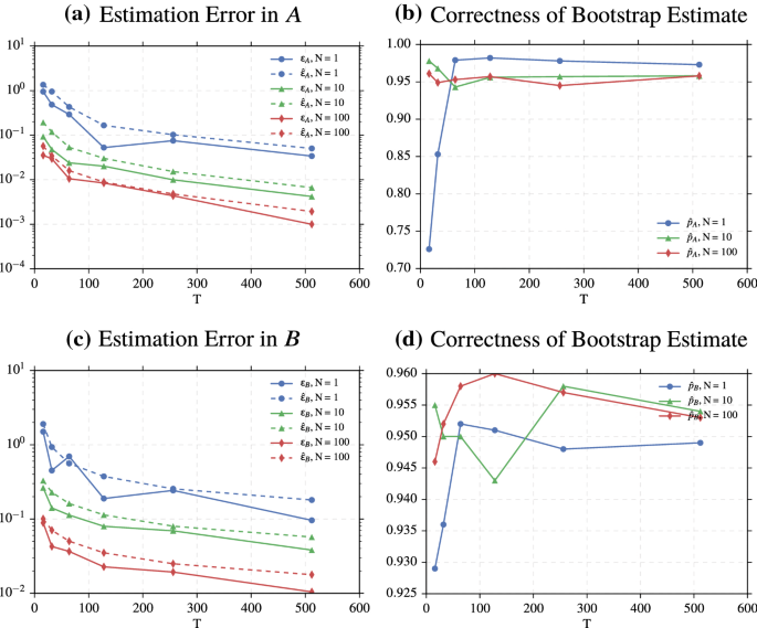
We evaluate the efficacy of the bootstrap procedure introduced in Algorithm 2. Recall that even though we provide theoretical bounds in Proposition 1, for practical purposes and for handling dependent data, we want bounds that are the least conservative possible.

For given state dimension $n$, input dimension $p$, and scalar $\rho$, we generate upper triangular matrices $A\in {\mathbb {R}}^{n\times n}$ with all diagonal entries equal to $\rho$ and the upper triangular entries i.i.d. samples from ${\mathcal {N}}(0,1)$, clipped at magnitude 1. By construction, matrices will have spectral radius $\rho$. The entries of $B\in {\mathbb {R}}^{n\times p}$ were sampled i.i.d. from ${\mathcal {N}}(0,1)$, clipped at magnitude 1. The variance terms $\sigma _u^2$ and $\sigma _w^2$ were fixed to be 1.

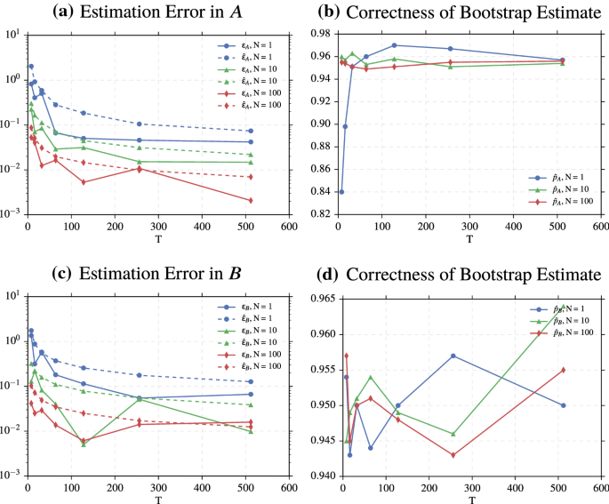
Recall from Sect. 2.3 that M represents the number of trials used for the bootstrap estimation, and ${{\widehat{\epsilon }}}_A$, ${{\widehat{\epsilon }}}_B$ are the bootstrap estimates for $\epsilon _A$, $\epsilon _B$. To check the validity of the bootstrap procedure, we empirically estimate the fraction of time $A$ and $B$ lie in the balls $B_{{\widehat{A}}}({\widehat{\epsilon }}_A)$ and $B_{{\widehat{B}}}({\widehat{\epsilon }}_B)$, where $B_{X}(r) = \{X':\Vert X' - X \Vert _2 \le r\}$.

Our findings are summarized in Figs. 5 and 6. Although not plotted, the theoretical bounds found in Sect. 2 would be orders of magnitude larger than the true $\epsilon _A$ and $\epsilon _B$, while the bootstrap bounds offer a good approximation.

Fig. 5

In these simulations: $n= 3$, $p= 1$, $\rho = 0.9$, and $M = 2000$. In (a), the spectral distances to $A$ (shown in the solid lines) are compared with the bootstrap estimates (shown in the dashed lines). In (b), the probability $A$ lies in $B_{{\widehat{A}}}({\widehat{\epsilon }}_A)$ estimated from 2000 trials. In (c), the spectral distances to $B_*$ are compared with the bootstrap estimates. In (d), the probability $B$ lies in $B_{{\widehat{B}}}({\widehat{\epsilon }}_B)$ estimated from 2000 trials

Fig. 6

In these simulations: $n= 6$, $p= 2$, $\rho = 1.01$, and $M = 2000$. In (a), the spectral distances to $A$ are compared with the bootstrap estimates. In (b), the probability $A$ lies in $B_{{\widehat{A}}}({\widehat{\epsilon }}_A)$ estimated from 2000 trials. In (c), the spectral distances to $B$ are compared with the bootstrap estimates. In (d), the probability $B$ lies in $B_{{\widehat{B}}}({\widehat{\epsilon }}_B)$ estimated from 2000 trials

Experiments with Varying Rollout Lengths

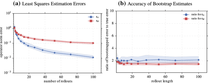
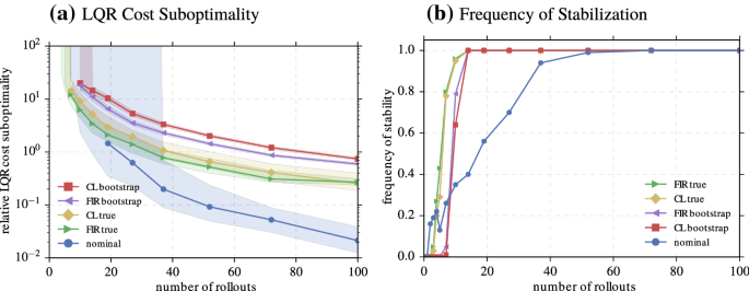
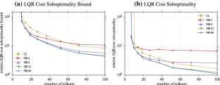
Here we include results of experiments in which we fix the number of trials ($N=6$) and vary the rollout length. Figure 7 displays the estimation errors. The estimation errors on $A$ decrease more quickly than in the fixed rollout length case, consistent with the idea that longer rollouts of easily excitable systems allow for better identification due to higher signal-to-noise ratio. Figure 8 shows that stabilizing performance of the nominal is somewhat better than in the fixed rollout length case (Fig. 2). This fact is likely related to the smaller errors on the estimation of $A$ (Fig. 7).

Fig. 7

The resulting errors from 100 identification experiments with a total of $N=6$ rollouts are plotted against the length rollouts. In (a), the median of the least squares estimation errors decreases with T. In (b), the ratio of the bootstrap estimates to the true estimates. Shaded regions display quartiles

Fig. 8

Performance of controllers synthesized on the results of the 100 identification experiments is plotted against the length of rollouts. In (a), the median sub-optimality of nominal and robustly synthesized controllers are compared, with shaded regions displaying quartiles, which go off to infinity when stabilizing controllers are not frequently found. In (b), the frequency synthesis methods found stabilizing controllers

References

Y. Abbasi-Yadkori and C. Szepesvári. Regret Bounds for the Adaptive Control of Linear Quadratic Systems. In Proceedings of the 24th Annual Conference on Learning Theory, pages 1–26, 2011.
M. Abeille and A. Lazaric. Thompson sampling for linear-quadratic control problems. In AISTATS 2017-20th International Conference on Artificial Intelligence and Statistics, 2017.
M. Abeille and A. Lazaric. Improved regret bounds for thompson sampling in linear quadratic control problems. In International Conference on Machine Learning, pages 1–9, 2018.
J. Anderson and N. Matni. Structured state space realizations for sls distributed controllers. In 2017 55th Annual Allerton Conference on Communication, Control, and Computing (Allerton), pages 982–987. IEEE, 2017.
M. ApS. The MOSEK optimization toolbox for MATLAB manual. Version 8.1 (Revision 25)., 2015. URL http://docs.mosek.com/8.1/toolbox/index.html.
F. Borrelli, A. Bemporad, and M. Morari. Predictive control for linear and hybrid systems. Cambridge University Press, New York, NY, USA, 2017.
G. E. Box, G. M. Jenkins, G. C. Reinsel, and G. M. Ljung. Time series analysis: forecasting and control. John Wiley & Sons, 2015.
R. P. Braatz, P. M. Young, J. C. Doyle, and M. Morari. Computational complexity of \(\mu \) calculation. IEEE Transactions on Automatic Control, 39 (5): 1000–1002, 1994.
S. J. Bradtke, B. E. Ydstie, and A. G. Barto. Adaptive linear quadratic control using policy iteration. In Proceedings of 1994 American Control Conference-ACC’94, volume 3, pages 3475–3479. IEEE, 1994.
M. C. Campi and E. Weyer. Finite sample properties of system identification methods. IEEE Transactions on Automatic Control, 47 (8): 1329–1334, 2002.
J. Chen and G. Gu. Control-Oriented System Identification: An \(\cal{H}_\infty \) Approach. Wiley, 2000.
J. Chen and C. N. Nett. The Caratheodory-Fejer problem and \(H_\infty \) identification: a time domain approach. In Proceedings of 32nd IEEE Conference on Decision and Control, pages 68–73. IEEE, 1993.
M. A. Dahleh and I. J. Diaz-Bobillo. Control of uncertain systems: a linear programming approach. Prentice-Hall, Inc., Upper Saddle River, NJ, USA, 1994.
S. Dean, S. Tu, N. Matni, and B. Recht. Safely Learning to Control the Constrained Linear Quadratic Regulator. arXiv:1809.10121, 2018.
J. Doyle. Analysis of feedback systems with structured uncertainties. IEE Proceedings D - Control Theory and Applications, 129(6), 1982. ISSN 0143-7054. https://doi.org/10.1049/ip-d.1982.0053.
Y. Duan, X. Chen, R. Houthooft, J. Schulman, and P. Abbeel. Benchmarking deep reinforcement learning for continuous control. In International Conference on Machine Learning, pages 1329–1338, 2016.
B. Dumitrescu. Positive trigonometric polynomials and signal processing applications, volume 103. Springer Science & Business Media, 2007.
B. Efron. Bootstrap Methods: Another Look at the Jackknife, pages 569–593. Springer New York, New York, NY, 1992. https://doi.org/10.1007/978-1-4612-4380-9_41.
M. K. H. Fan, A. L. Tits, and J. C. Doyle. Robustness in the presence of mixed parametric uncertainty and unmodeled dynamics. IEEE Transactions on Automatic Control, 36(1), 1991. ISSN 0018-9286. https://doi.org/10.1109/9.62265.
M. Fazel, R. Ge, S. Kakade, and M. Mesbahi. Global convergence of policy gradient methods for the linear quadratic regulator. In Proceedings of the 35th International Conference on Machine Learning, volume 80, pages 1467–1476. PMLR, 10–15 Jul 2018.
E. Feron. Analysis of robust \({\cal{H}}_2\) performance using multiplier theory. SIAM Journal on Control and Optimization, 35 (1): 160–177, 1997. 10.1137/S0363012994266504.
C.-N. Fiechter. PAC adaptive control of linear systems. In Proceedings of the Tenth Annual Conference on Computational Learning Theory, COLT ’97, pages 72–80, New York, NY, USA, 1997. ACM. https://doi.org/10.1145/267460.267481.
A. Goldenshluger. Nonparametric estimation of transfer functions: rates of convergence and adaptation. IEEE Transactions on Information Theory, 44 (2): 644–658, 1998. https://doi.org/10.1109/18.661510.
A. Goldenshluger and A. Zeevi. Nonasymptotic bounds for autoregressive time series modeling. Ann. Statist., 29 (2): 417–444, 04 2001. 10.1214/aos/1009210547.
P. Hall. The Bootstrap and Edgeworth Expansion. Springer Science & Business Media, 2013.
M. Hardt, T. Ma, and B. Recht. Gradient descent learns linear dynamical systems. The Journal of Machine Learning Research, 19 (1): 1025–1068, 2018.
E. Hazan, K. Singh, and C. Zhang. Learning linear dynamical systems via spectral filtering. In Advances in Neural Information Processing Systems, pages 6702–6712, 2017.
E. Hazan, H. Lee, K. Singh, C. Zhang, and Y. Zhang. Spectral filtering for general linear dynamical systems. In Advances in Neural Information Processing Systems, pages 4634–4643, 2018.
A. J. Helmicki, C. A. Jacobson, and C. N. Nett. Control oriented system identification: a worst-case/deterministic approach in \(\cal{H}_\infty \). IEEE Transactions on Automatic Control, 36 (10): 1163–1176, 1991. 10.1109/9.90229.
M. Ibrahimi, A. Javanmard, and B. V. Roy. Efficient reinforcement learning for high dimensional linear quadratic systems. In F. Pereira, C. J. C. Burges, L. Bottou, and K. Q. Weinberger, editors, Advances in Neural Information Processing Systems 25, pages 2636–2644, 2012.
N. Jiang, A. Krishnamurthy, A. Agarwal, J. Langford, and R. E. Schapire. Contextual decision processes with low Bellman rank are PAC-learnable. In Proceedings of the 34th International Conference on Machine Learning, volume 70, pages 1704–1713. PMLR, 06–11 Aug 2017.
E. Jonas, Q. Pu, S. Venkataraman, I. Stoica, and B. Recht. Occupy the cloud: Distributed computing for the 99%. In Proceedings of the 2017 Symposium on Cloud Computing, pages 445–451. ACM, 2017. 10.1145/3127479.3128601.
V. Kuznetsov and M. Mohri. Generalization bounds for non-stationary mixing processes. Machine Learning, 106 (1): 93–117, 2017. https://doi.org/10.1007/s10994-016-5588-2.
S. Levine, C. Finn, T. Darrell, and P. Abbeel. End-to-end training of deep visuomotor policies. Journal of Machine Learning Research, 17 (1): 1334–1373, Jan. 2016.
W. Li and E. Todorov. Iterative Linear Quadratic Regulator Design for Nonlinear Biological Movement Systems. In International Conference on Informatics in Control, Automation and Robotics, 2004.
L. Ljung. System Identification: Theory for the User. Prentice-Hall, Inc., Upper Saddle River, NJ, USA, 1999.
J. Löfberg. YALMIP : A toolbox for modeling and optimization in MATLAB. In IEEE International Symposium on Computer Aided Control System Design, 2004.
N. Matni, Y. Wang, and J. Anderson. Scalable system level synthesis for virtually localizable systems. In 2017 IEEE 56th Annual Conference on Decision and Control (CDC), pages 3473–3480, Dec 2017. https://doi.org/10.1109/CDC.2017.8264168.
D. J. McDonald, C. R. Shalizi, and M. Schervish. Nonparametric risk bounds for time-series forecasting. Journal of Machine Learning Research, 18 (1): 1044–1083, Jan. 2017.
A. Megretski and A. Rantzer. System analysis via integral quadratic constraints. IEEE Transactions on Automatic Control, 42(6): 819–830, June 1997. https://doi.org/10.1109/9.587335.
V. Mnih, K. Kavukcuoglu, D. Silver, A. A. Rusu, J. Veness, M. G. Bellemare, A. Graves, M. Riedmiller, A. K. Fidjeland, G. Ostrovski, S. Petersen, C. Beattie, A. Sadik, I. Antonoglou, H. King, D. Kumaran, D. Wierstra, S. Legg, and D. Hassabis. Human-level control through deep reinforcement learning. Nature, 518: 529–533, 02 2015.
M. Mohri and A. Rostamizadeh. Stability bounds for stationary \(\phi \)-mixing and \(\beta \)-mixing processes. Journal of Machine Learning Research, 11: 789–814, 2010.
Y. Ouyang, M. Gagrani, and R. Jain. Control of unknown linear systems with thompson sampling. In 2017 55th Annual Allerton Conference on Communication, Control, and Computing (Allerton), pages 1198–1205, Oct 2017. https://doi.org/10.1109/ALLERTON.2017.8262873.
A. Packard and J. Doyle. The complex structured singular value. Automatica, 29 (1): 71 – 109, 1993. https://doi.org/10.1016/0005-1098(93)90175-S.
F. Paganini. Necessary and sufficient conditions for robust \({\cal{H}}_2\) performance. In Proceedings of 1995 34th IEEE Conference on Decision and Control, volume 2, pages 1970–1975 vol.2, Dec 1995. https://doi.org/10.1109/CDC.1995.480635.
J. Pereira, M. Ibrahimi, and A. Montanari. Learning networks of stochastic differential equations. In Advances in Neural Information Processing Systems, pages 172–180, 2010.
R. Postoyan, L. Buşoniu, D. Nešić, and J. Daafouz. Stability analysis of discrete-time infinite-horizon optimal control with discounted cost. IEEE Transactions on Automatic Control, 62 (6): 2736–2749, June 2017. https://doi.org/10.1109/TAC.2016.2616644.
L. Qiu, B. Bernhardsson, A. Rantzer, E. Davison, P. Young, and J. Doyle. A formula for computation of the real stability radius. Automatica, 31 (6): 879 – 890, 1995. https://doi.org/10.1016/0005-1098(95)00024-Q.
D. J. Russo, B. Van Roy, A. Kazerouni, I. Osband, and Z. Wen. A tutorial on thompson sampling. Foundations and Trends on Machine Learning, 11(1): 1–96, 2018. https://doi.org/10.1561/2200000070.
J. Shao and D. Tu. The Jackknife and Bootstrap. Springer Science & Business Media, 2012.
D. Silver, A. Huang, C. J. Maddison, A. Guez, L. Sifre, G. van den Driessche, J. Schrittwieser, I. Antonoglou, V. Panneershelvam, M. Lanctot, S. Dieleman, D. Grewe, J. Nham, N. Kalchbrenner, I. Sutskever, T. Lillicrap, M. Leach, K. Kavukcuoglu, T. Graepel, and D. Hassabis. Mastering the game of go with deep neural networks and tree search. Nature, 529: 484–489, 01 2016.
M. Simchowitz, H. Mania, S. Tu, M. I. Jordan, and B. Recht. Learning without mixing: Towards a sharp analysis of linear system identification. In Proceedings of the 31st Conference On Learning Theory, volume 75, pages 439–473. PMLR, 06–09 Jul 2018.
M. Sznaier, T. Amishima, P. Parrilo, and J. Tierno. A convex approach to robust \({\cal{H}}_2\) performance analysis. Automatica, 38 (6): 957 – 966, 2002. https://doi.org/10.1016/S0005-1098(01)00299-0.
S. Tu, R. Boczar, A. Packard, and B. Recht. Non-Asymptotic Analysis of Robust Control from Coarse-Grained Identification. arXiv:1707.04791, 2017.
A. W. Van Der Vaart and J. A. Wellner. Weak Convergence and Empirical Processes. Springer Science & Business Media, 1996.
R. Vershynin. Introduction to the non-asymptotic analysis of random matrices. arXiv:1011.3027, 2010.
M. Vidyasagar and R. L. Karandikar. A learning theory approach to system identification and stochastic adaptive control. Journal of Process Control, 18 (3): 421 – 430, 2008. https://doi.org/10.1016/j.jprocont.2007.10.009.
M. J. Wainwright. High-Dimensional Statistics: A Non-Asymptotic Viewpoint. Cambridge Series in Statistical and Probabilistic Mathematics. Cambridge University Press, 2019. https://doi.org/10.1017/9781108627771.
Y. Wang, N. Matni, and J. C. Doyle. A system level approach to controller synthesis. IEEE Transactions on Automatic Control, pages 1–1, 2019. https://doi.org/10.1109/TAC.2018.2890753.
F. Wu and A. Packard. Optimal lqg performance of linear uncertain systems using state-feedback. In Proceedings of 1995 American Control Conference - ACC’95, volume 6, pages 4435–4439, June 1995. https://doi.org/10.1109/ACC.1995.532775.
D. Youla, H. Jabr, and J. Bongiorno. Modern wiener-hopf design of optimal controllers–part ii: The multivariable case. IEEE Transactions on Automatic Control, 21 (3): 319–338, 1976. https://doi.org/10.1109/TAC.1976.1101223.
P. M. Young, M. P. Newlin, and J. C. Doyle. \(\mu \) analysis with real parametric uncertainty. In Proceedings of the 30th IEEE Conference on Decision and Control, volume 2, pages 1251–1256, Dec 1991. https://doi.org/10.1109/CDC.1991.261579.
B. Yu. Rates of convergence for empirical processes of stationary mixing sequences. The Annals of Probability, 22 (1): 94–116, 1994.
K. Zhou, J. C. Doyle, and K. Glover. Robust and Optimal Control. Prentice-Hall, Inc., Upper Saddle River, NJ, USA, 1996.
Acknowledgements
We thank Ross Boczar, Qingqing Huang, Laurent Lessard, Michael Littman, Manfred Morari, Andrew Packard, Anders Rantzer, Daniel Russo, and Ludwig Schmidt for many helpful comments and suggestions. We also thank the anonymous referees for making several suggestions that have significantly improved the paper and its presentation.
Author information
Authors and Affiliations
Corresponding author
Additional information
Communicated by Michael Overton.
Publisher's Note
Springer Nature remains neutral with regard to jurisdictional claims in published maps and institutional affiliations.
This work was generously supported in part by NSF award CCF-1359814, ONR awards N00014-14-1-0024 and N00014-17-1-2191, the DARPA Fundamental Limits of Learning Program, a Sloan Research Fellowship, and a Google Faculty Award. SD is additionally supported by an NSF Graduate Research Fellowship under Grant No. DGE 1752814. NM is additionally supported by grants from the AFOSR and NSF, and by gifts from Huawei and Google.