
Abstract
Two simulation experiments were conducted to verify whether the idea of virtual force scatter plot algorithm, used for searching solutions of the facility layout problems, may be used as an input to the classical CRAFT and simulated annealing (SA) algorithms. The proposed approach employs a regular grid for specifying possible locations of objects. Three independent variables were investigated in the first experiment, namely, (1) the size of the problem: 16, 36 and 64 objects, (2) the type of links between objects: grid, line, and loop, and (3) the shape of the possible places in which the objects can be situated: circle, row and square. The patterns of possible location places were also adapted to the analysis of examples taken from literature, included in the second experiment. The gathered data were statistically analyzed. The results shows substantial decrease in goal function means for all of the examined experimental conditions, if the proposed starting solutions are applied to the CRAFT algorithm. The application of the approach to SA is profitable in specific tasks. The presented comparative numerical results show, in which circumstances the proposed method is superior over various genetic algorithms and other hybrid approaches. Overall, the experimental data investigation demonstrates the usefulness of the proposed method and encourages further research in this direction.
1 Introduction
Generally, the facility layout problem (FLP) deals with looking for the best arrangement of objects in available places, subject to existing relationships between objects and various constraints. The problem is certainly of major interest for scientists and practitioners from such areas as logistics, production engineering, or ergonomic workplace design. The main purpose of facilities layout optimization in these areas is the costs minimization of their common functioning. In industrial engineering and, particularly, in logistics, one looks for such locations of machinery, equipment and workplaces in the production space, that ensures material handling and employees’ movement costs minimization.
Facilities layout models may be used in many practical human factors and ergonomics studies for optimizing individual workplaces, especially man–machine interactions. An optimal interface allows for minimizing psychophysical cost of an operator functioning in the man–machine system, by providing best possible locations of control and information devices, in relation to themselves and to the human-being. Optimization criteria in this field often cover the number and the quality of necessary body movements, extremities moves as well as human visual system engagement (e.g., the number and duration of fixations and saccades). Concepts and optimization models in these areas are presented, for instance, in the works of Sargent et al. (1997), Holman et al. (2003), Paquet and Lin (2003), Lin and Wu (2010) and Jung et al. (2012). In the domain of human resources management, mutual locations of persons in, e.g., an open space office, based on frequency of their necessary contacts, can rationalize company’s processes. Optimization of employees’ work places can also be performed by taking into account informal contacts extracted from the socio-matrix, called the Moreno matrix (Moreno 1934). Various types of such matrices are described in Klüver and Stoica (2003). Tompkins and White, already in 1984, specified a number of various types of relationships that could be used as inputs to the facilities layout problem. They identified relationships regarding the following areas: facilities, flow, control, process and service, organization and personnel, environment.
Though the facilities layout concept seems to be simple, it has been shown (Sahni and Gonzalez 1976) that the optimal solution cannot be obtained in polynomial time, which means that the FLP belongs at least to the class of NP-complete problems. As a result, a number of diverse heuristic approaches have been elaborated. They search for acceptable solutions in reasonable time for problems involving many objects. Systematic and comprehensive reviews of developments and advancements in this regard are provided, for instance, by Kusiak and Heragu (1987), Meller and Gau (1996), Singh and Sharma (2006), Drira et al. (2007), or Moslemipour et al. (2012).
1.1 Hybrid approaches and initial solutions
In approaches classified as improvement algorithms, as well as in most metaheuristics, final solutions depend, to a significant extent, on initial conditions. These initial solutions are generated for traditional algorithms, usually, at random. The need for developing heuristics for creating better starting points is rational and was suggested, among others, by Singh and Sharma (2006), and Drira et al. (2007). One of the first proposals in this trend was demonstrated by Liggett (1981). He showed that a combination of the improvement procedure (a variation of the classical pair exchange algorithm), starting from the initial construction solution, provides better results than for a random starting solution. However, the effectiveness of hybrid algorithms depended on the nature of the relationships matrix. The author examined problems widely known in the literature, introduced by Steinberg (1961) and Nugent et al. (1968), which differed considerably in their flow dominance (FD) values (Vollmann and Buffa 1966). This indicator is computed by dividing the standard deviation of the relationships matrix values by their average. It reflects the variability of the relationships level and, thus, shows how strong the results may be influenced by changes in location of objects, strongly or weakly connected with others. The Liggett’s experimental results demonstrated that the quality of the FLP with a low flow dominance indicator increases, if the hybrid approach is applied. When the flow dominance is high, the construction algorithm gives results that can hardly be improved.
A comparison of 12 algorithms made by Kusiak and Heragu (1987), demonstrated the dominance of four hybrid algorithms in solving Nugent’s et al. (1968) test problems having small flow dominance value over construction and improvement type algorithms with random initial solutions. The solution quality criterion in this work was computed by dividing the goal function value by the lower bound, and expressed in percentages. For instance, for the 30 objects’ problem solved by construction and improvement (CRAFT) methods, the quality criterion amounted to 142.5%. The hybrid facility layout by analysis of clusters (FLAC) approach (Scriabin and Vergin 1985) allowed for obtaining a much better value of 137.6%.
Apart from hybrid approaches that link various improvement algorithms based on changing pairs with different ways of obtaining initial solutions, there are also hybrid techniques involving the SA metaheuristic (Kirkpatrick et al. 1983). The SA is similar to improvement methods in that, it is based on a gradual enhancement of the goal function but allows for changes to the worse. Thanks to this feature, it may avoid the entrapment in one local minimum. Originally, and in first applications to FLP (Burkard and Rendl 1984; Wilhelm and Ward 1987), SA starts from a random initial solution. Heragu and Alfa (1992) proposed a two-stage algorithm in which the initial solution is generated by a modified penalty (MP) algorithm and only then, SA is applied. A combination of MP and SA proved to be successful as it produced many best solutions to FLP benchmarks problems those days. Similar hybrid approach was published by Singh and Sharma (2008). Their SA application was tested on a widely known Nugent’s et al. (1968) FLP, and occurred to be better than many previous ones. Various hybrid approaches including SA are still being developed. Recently, for instance, Leitold et al. (2018) proposed an algorithm integrating SA and dynamic programming for working time line balancing.
Initial solutions’ generation is also subject to examination by some authors of the latest genetic algorithms. For instance, Liu and Sun (2012) used cluster analysis for creating initial chromosomes’ structures in the first generation of solutions. Their experimental research outcomes showed that this approach provides better results than previous genetic algorithms. Another idea of creating initial chromosomes for a classical genetic algorithm, was put forward by Sadrzadeh (2012). In this case, the facilities with stronger relationships are grouped together. The grouping is used in heuristic crossover and mutation operators. The author demonstrated that his proposal generates better results for two FLP examples, solved earlier by algorithms employing random starting solutions. Moreover, the Sadrzadeh (2012) technique yielded the best known solution for the FLP presented in the Kazerooni et al. (1995) work. Lately, the idea of using other than random starting solutions is applied in many other hybrid approaches, e.g., Kierkosz and Luczak (2014), Hiermann, et al. (2015), or Ranjbar et al. (2018).
1.2 Scatter plot concepts
Unlike other concepts, scatter plot approaches allow for unconstrained location of objects on a plane, instead of placing them in predefined places. Thus, the solution is presented in a form of irregular shapes resembling scatter plots. Objects’ adjacencies in this type of algorithm correspond to objects’ relationships. The idea of scattered plots was originally put forward by Drezner in the article published in 1980 and later developed and analyzed in his further works from 1987 and 2010. In Drezner’s deterministic algorithm for finding optimal scatter plots, the final objects’ coordinates are computed by means of eigenvectors of the specifically transformed flow-matrix.
Similar idea was also proposed by Scriabin and Vergin (1985). In their hybrid approach, they used the modified multidimensional scaling method for finding initial solutions. The multidimensional scaling is usually used for conducting cluster analyses of data structures and is based on finding eigenvectors of the matrix containing dissimilarities between items. In the Scriabin and Vergin (1985) approach the dissimilarities’ matrix was constructed based on the objects’ relationships array.
Another algorithm in this trend was presented by Grobelny (1999). In his approach, the scattered plot is generated by mimicking physical processes in which the final state results from two different forces acting on every object, placed initially at the center of a plane. One vector starts from the center of the plane and, in the first step, is directed towards a randomly chosen point on the plane. The second force depends on strengths of connections with other items. The resultant vectors of these two forces specify positions of objects in the next step. The final scatter plot is produced by repeatedly calculating these forces for all objects, and moving them to their new locations. Since one of the components of the movement direction vector is determined at random, every solution is different but in all cases the objects’ mutual relationships are conserved.
2 The goal and contribution of the research
As it was mentioned in the literature review, heuristics often seem to be sensitive both to the input data structure, and starting conditions. Thus, in this paper, we propose the idea of using virtual force algorithm generated scatter plots (Grobelny 1999) as initial solutions for two regular modular-grid-based facility layout optimization algorithms, namely CRAFT and SA. We additionally, show in which circumstances such an approach is especially useful.
Effectiveness and optimization results quality of this proposal are thoroughly examined for various types of typical models of production and ergonomic systems as well as practical FLP analyzed extensively in the literature. For this purpose, two simulation experiments were designed and conducted:
The first experiment involves systematic investigation of classic production and maintenance processes with known optimal goal function values. They include diverse number of objects, structures of the relationships matrix, and layouts of possible locations of objects.
In the second experiment, the proposed hybrid approach is applied to various real-life FLPs taken from literature, for which the best known solutions were available. To compare our results with the previous ones we chose only regular-grid-based examples. We analyze the practical problems not only on their original layouts but also in configurations used in the first experiment.
All the data from both simulation experiments are formally, statistically compared with solutions obtained when the initial arrangement is generated randomly. The obtained results show a significant advantage of the proposed hybrid approach over the classical one, where the starting solution is randomly generated. In particular:
Applying the scatter plot algorithm with CRAFT provided optimal solutions in most of the conditions examined in the first experiment, and best known results in the second experiment. In all cases solutions obtained by our approach were better than those with random initial layouts.
Scatter plots with SA generated better than randomly initialized results for specific relations between input data and the production system structure. The proposed hybrid approach not only systematically provides optimal and/or best results, but also is stable which manifests itself by smaller values of MSDs.
3 Methodology
3.1 CRAFT and simulated annealing implementations
3.1.1 Craft
In this study, the CRAFT version proposed in the work of Buffa et al. (1964) was employed. Generally, this relatively simple, and well known algorithm is based on either two way or three way exchanges of objects’ locations. The procedure involves examining all possible changes at each step, and identifying the best one in terms of improving the goal function value. Then, the current layout is updated, and in the next step, again, all possible exchanges are considered. The whole procedure is repeated until it is not possible to obtain any improvement of the goal function value. The classical implementation starts from a random distribution of objects, on a regular grid, where the distance between adjacent objects amounts to one. In our implementation, we included pairwise changes of objects’ locations.
3.1.2 Simulated annealing
The SA algorithm was implemented in accordance with the idea put forward, for the first time, in the seminal paper of Kirkpatrick et al. (1983) that was directly inspired by the article of Metropolis et al. (1953). In general, the procedure is based on imitating the metal particles’ movements during the annealing process. In the algorithm, the movement is simulated by changing places of objects’ locations, and involves either pairs or triplets. The process runs in a changeable temperature (T) which is decreased in every step. If, in a given step, the change in objects’ places improves the solution then it is accepted. However, even if the change does not decrease the goal function value, it can still be accepted with the following probability P:
where ∆ denotes the value by which the goal function would be increased by this specific change of objects places. In other words, the greater the value of ∆, the greater is the probability of this solution being rejected. This is known as the Metropolis acceptance rule (Metropolis et al. 1953), which implies that the smaller the increase of the ∆ value, the more likely the new solution is selected, and the lower the value of T (and greater the number of trials), the less likely the given solution is accepted (Heragu and Alfa 1992).
The practical SA implementation requires defining the initial temperature (Ti), the epoch length, the cooling (annealing) schedule, and the termination criterion. The review of various approaches to specifying these parameters is presented by Singh and Sharma (2008), and our SA version is based on these experiences.
Kirkpatrick et al. (1983) recommend accepting worse solutions with the probability of about 0.8 in the first step of the SA procedure. To conform to this suggestion, we used the idea of computing the initial temperature Ti based on the assumed probability and the approximated average ∆ value for a given FLP. The value is established by performing N2 (N is the number of all objects) random changes of objects pairs and computing the mean value of ∆’s. A similar approach was also used by Singh and Sharma (2008).
The number of repetitions (objects’ pair changes) in a given temperature (the epoch length) was proportional to the number of objects in a problem y × N (where y is a multiplicative coefficient). Analogous solution was applied in the works of Wilhelm and Ward (1987) or Heragu and Alfa (1992).
The cooling scheme was specified like in the paper of Heragu and Alfa (1992), namely Tj = r × Tj−1, with r = 0.9. The final temperature Tf is computed taking into account the assumed number of steps i according to the formula Tf = 0.9(i−1) × Ti. Thus, reaching the final temperature which is achieved after performing the specified number of steps, is the stopping criterion.
A number of preliminary runs of the SA algorithm for experimental conditions, where optimal or best solutions are known, allowed for setting the reasonable values for the remaining two parameters. As a result of these observations i was set at 100 while y at 10.
3.2 Initial solution based on scatter plot generation
The idea of the Links algorithm, originally proposed by Grobelny (1999), is based on a simulation of the physical process inspired by the big bang. All objects at the beginning of the simulation are located in the middle of a square piece of a plane. Then, a randomly chosen target point on a plane is assigned to each item. During next steps, every object moves towards a direction which is a sum of the following two vectors of forces:
A dispersing force vector acting along straight line from the middle to a given object is proportional to maximal value in the relationships matrix and a current distance to the randomly determined value in the first step of the algorithm. Also, in the first step, a random target point is assigned to each object, and they move towards these targets by a distance equal to 1% of the plane diagonal length.
An attracting force vector acting towards other objects being a sum of vectors, directed towards every other object and proportional to relationship values with these objects and distances between them. The situation between a pair of objects resembles the model of ideal spring, where the relationship between these objects corresponds to the string stiffness constant.
The geometric idea of how the procedure works is illustrated in Fig. 1, where AB is a vector of the force proportional to the link between A and B from Table 1; AC denotes a vector of the force proportional to the link between A and C; ABC is the sum of vectors AB and AC; AP is a vector of the force proportional to the maximal value of links from Table 1, directed along the straight line, from the plane center (PC) to the object’s center, and proportional to the distance between the object’s center, and the distance value randomly generated in the first step; F denotes the sum of all vectors in a given step which specifies the movement direction in the next step.

The geometric illustration of determining the force F influencing the A object movement in a given step
Based on an only very simple example with three objects having relationships presented in Table 1, the graphics demonstrates the way of obtaining the resultant force vector for the A object at a given step of the procedure.
Every object has a circular buffer zone specified as a percentage of the plane dimension. This concept allows taking into account approximate objects’ dimensions. If any object enters this zone the attraction force between these objects stops working. The same mechanism is also applied to distances randomly chosen in the first step. The final distribution of objects on the plane is obtained when neither of objects moves or after the specified number of steps.
The obtained solution depends naturally on the relationship matrix. Generally, the algorithm will tend to place objects with strong relationships close to each other. Given big discrepancies between relationship matrices, such as their extremely different flow dominance values, it was necessary to introduce additional two parameters controlling the objects’ movements: (i) the coefficient specifying a single step distance covered by the object when the unit force vector is applied, and (ii) the relative weights of the dispersing and attracting forces used in the procedure: α and 1 − α, where α takes the values between 0 and 1. The latter coefficients have particular meaning for diverse structures of relationships and their values. For instance, when the FD value is small, which indicates big density of connections between objects along with small variability of their relationships levels, the attracting vector is usually directed towards the center of the group. In this situation, to obtain a reasonable scatter plot solution, the dispersing vector should be relatively stronger to counterbalance the mutual objects’ attractions. In the current research, the abovementioned parameters were determined by means of the trial and error technique.
3.3 Assigning scatter plot results to regular grids
After performing the Links procedure, it is necessary to convert the obtained solution to the regular grid structure characteristic of the CRAFT and SA algorithms. A similar operation was also necessary in the work of Scriabin and Vergin (1985). In this study, two methods were developed to cope with this problem. In the first approach, we simply successively assigned objects to the nearest empty cell in a regular grid which was superimposed on the earlier obtained scatter plot. The second technique is the extension of the first one. The assignment procedure is repeated after rotating the scatter plot solution plane around its center by the specified angle. In this study, the rotation by 5° was applied. Preliminary simulations proved that this value was a good compromise between the speed and obtaining decent goal function values. From among all of the obtained assignments, the one with the best goal function value is finally accepted. The procedures are illustrated in Figs. 2, 3 and 4.

The assignment procedure of the exemplary scatter plot solution to the regular grid

The assignment order procedure of objects from Fig. 2 after the 45° rotation

The final solution obtained for the 45° rotated scattered plane from the example demonstrated in Fig. 3
3.4 Dependent measures
In all experiments, the following objective function was used as a dependent measure:
where Dp(i)p(j) is obtained according to the Minkowski metric formula (cf. Wikipedia 2019):
where k denotes the dimension and r specifies the particular metric. The latter parameter amounts to one in the current research. This metric is also called rectilinear, city block, or Manhattan. The Lij shows the relationship strength between the given pair of objects.
4 Simulation experiments
All the algorithms and simulation experiments were implemented and run in Borland Delphi 2005, version 9.0.
4.1 Experiment 1: typical models of production layouts
4.1.1 Independent variables
Three factors were manipulated as the independent variables, that is, (1) the objects’ available locations on the plane, (2) the structure of relationships between objects, and (3) the number of objects in the problem. The levels of these effects are specified in the following paragraphs.
Possible objects’ locations on the plane (OL). Theoretically, the number of available locations for objects is infinite. It is, naturally, not feasible to examine all possibilities, therefore, we restricted our study only to the layouts that have their significant practical meaning. In the current experiment, we focused on the structures reflecting typical organizations of material handling systems (Kusiak and Heragu 1987; Drira et al. 2007). Three geometrical layouts were taken into consideration, that is: (i) a single straight row arrangement (row, Fig. 5) characteristic, for instance, of the partly or fully automated production or assembly lines, Automated Guided Vehicle or a series of activities performed sequentially by a worker on a control panel, (ii) an open field having the rectangular (or square) shape (square, Fig. 6) typical for visual inspections of information panels or gantry robots in logistics and used when the available space is limited, and finally (iii) the circular arrangement, for example, commonly applied to work organized in cells or when material handling is based on logistics trains (circle, Fig. 7).
Fig. 5 
The single row layout for possible locations of 16 objects
Fig. 6 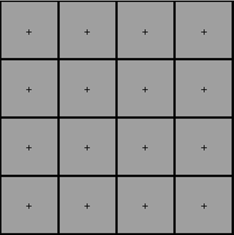
The square layout for 16 possible object locations
Fig. 7 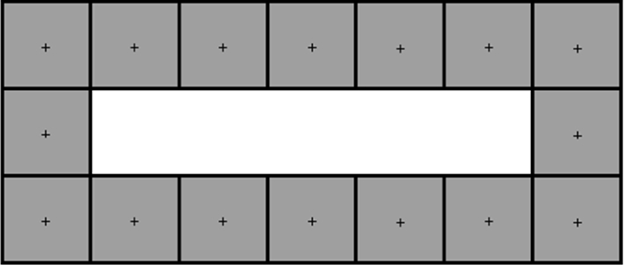
The circular layout for possible location of 16 objects
The relationship type between objects (RO). For each of the defined geometrical layout of possible objects’ locations, the objects’ links were specified in such a way that the optimal arrangements are known. Elaborated relationships’ matrices contained only values of zero and one and reflected either the situation when the adjacency of the two specific objects is required (1) or not (0). Three versions of objects’ relationships included: (i) the line structure (an example including 16 objects is presented in Fig. 8) designed for the single row layout, (ii) the grid type of relationships (Fig. 9) prepared for the square layout, and (iii) loop shaped links for the circle layout (Fig. 10).
Fig. 8 
Line type links for the 16 objects problem
Fig. 9 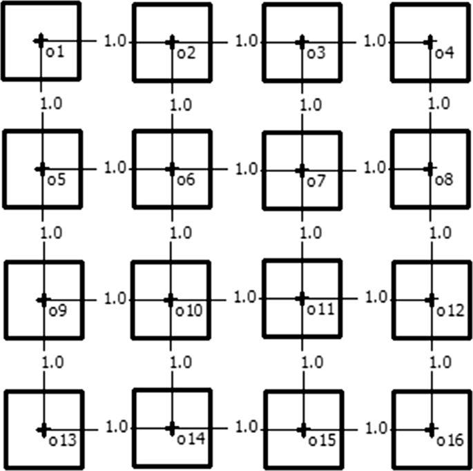
Grid type links for the 16 objects problem
Fig. 10 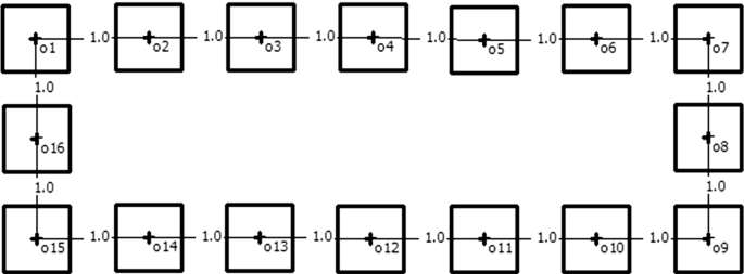
Loop type links for the 16 objects problem
The problem size (PS). As it was already mentioned the facility layout issues are difficult to solve optimally, so the problems considered in the literature include, usually, a moderate number of objects. There is a group of rather small problems having typically not more than a dozen or so items for which the optimal solution is known. Somewhat bigger practical problems are used as benchmarks for comparing the effectiveness and efficiency of various algorithms—they generally do not exceed 30 elements. Bigger problems are rarely used. Based on this analysis, and taking into account the nature of the possible location of objects specified in the first variable, we decided to investigate three types of problem sizes (PS): the small one including 16 objects, the medium—with 36 items and, finally, the large one involving as many as 64 elements.


4.1.2 Experimental design and procedure
A full experimental design was applied which means that all combinations of the factors’ levels were studied. Given the factors and their levels described above, 27 experimental test problems were produced: Objects layout (3) × Relationships type (3) × Problem size (3) = 27. The designed examples had a medium and high flow dominance value ranging from 2.0 to 5.6.
For each test problem, we examined the effectiveness of classical CRAFT and our implementation of SA algorithms, starting from three different initial solutions. These two algorithms were applied for (i) random initial layouts, (ii) layouts obtained by applying the Links algorithm followed by a simple conversion to regular grid (Links), and (iii) the conversion involving plane rotations (RotLinks). This produced six different simulation routines: Algorithm (2) × Initial solution (3). The simulations were repeated 100 times for each of Test problems (27) × Simulation routines (6) experimental conditions = 162. All goal function values along with the best layout obtained for a given experimental condition were recorded.
The Links algorithm parameters were determined after a series of pilot simulations, and were selected so that the algorithm was able to best reproduce desired layouts for the test problems with known optimal values. Figures 11 and 12 demonstrate layouts including 36 objects having the grid type of relationship obtained after performing the Links algorithm with different values of the attracting and dispersing force parameters. It can easily be observed that the solution from the second figure is more appropriate as it better reflects the grid nature of the connections between items.

Results of Links algorithm for a grid type links between 36 objects for scattering coefficients: 0.5 and 0.5

Results of Links algorithm for a grid type links between 36 objects for scattering coefficients: 0.2 and 0.8
For all experimental conditions the square plane was used and the following Links parameters were applied: the virtual force coefficient—10% of the plane dimension and dispersing/attracting force coefficients—0.2 and 0.8 respectively. The neutral zone was set at 5% of the plane dimension for all 16 objects examples and also for 36 and 64 objects examples with squared links connections. The value of neutral zone of 3% was found as the appropriate one for the 36 elements example with linear pattern links connections and 64 elements tasks having circular links patterns. For 64 elements tasks having a linear structure of connections, the neutral zone was fixed at 2% of the plane dimension.
4.1.3 Results and discussion
The basic descriptive statistics obtained in this experiment are put together in Table 2. Generally, the analysis of the results shows considerable improvements in average goal function values for the CRAFT algorithm, if the Links or RotLinks solutions, instead of the random one, were used as starting points. The results exhibit a similar pattern in all of the 27 test problems. Almost every time, the best mean result was registered when the RotLinks initial solution was applied. In couple of cases, the difference between outcomes obtained after Links and RotLinks procedures were statistically irrelevant. The relative discrepancies expressed in percentages between mean goal function values registered for different initial solutions are presented in Table 3. In the same table, statistical significances of differences were also provided.
The results of the Simulated Annealing algorithm were, on average, better than those obtained by the CRAFT algorithm. Only for small layouts with 16 items, the mean goal function values obtained by CRAFT with RotLinks initial solutions were not statistically worse than the solutions provided by SA. The influence of the better than random initial solutions on the final results is in most cases weak or none. However, in two cases, namely the combination of the grid type of relationships on a square layout with 36 and 64 objects, the improvement is large.
For 64 objects and the combination of the line type relationship and row type layout, the influence of initial solution is statistically significant.
Moreover, for the grid on the square test problem with 64 objects, the mean results obtained by CRAFT followed by RotLink are statistically significantly better than the average goal function values in SA for any type of initial solutions. The observed outcomes show that the effectiveness of examined initial solutions is limited when the SA is concerned and depends very much on the test problem structure. The best obtained solutions for each of examined test FLPs in Experiment 1 are provided in Supplementary material A.
4.2 Experiment 2: comparative analysis with examples from literature
4.2.1 Experimental design and procedure
In the first experiment we systematically examined various types of FLPs with a single value connections. Although we referred to layouts of practical significance, it seemed it would be interesting to investigate how CRAFT and our implementation of SA along with different types of initial solutions perform when applied to real life problems. Therefore, in the second experiment we focused on practical examples widely analyzed in the literature and frequently used as benchmarks. In the second experiment’s conditions we used original numbers of objects along with their relationships structures. Apart from possible locations used in studies reported in earlier papers, we also investigated additional layouts to obtain a variety of test problems similar to those examined in the first experiment. We chose four problems having various flow dominance values ranging from 1.1 to 4.2.
The first example was taken from the work of Chan and Tansri (1994) with the flow dominance value of 1.9. The optimal solution for this problem involving 9 elements on the square 3 × 3 grid is known. We also analyzed this case on the row and circle layouts. The second problem deals with placing 24 machines on the 5 × 6 rectangular grid and has the flow dominance value of 4.2, which is the biggest used in the current experiment. The data for this example was taken from Kazerooni et al. (1995). Just like in the previous case, apart from the original possible positions, we also examined row and circle layouts. The third problem was originally analyzed in the work of El-Baz (2004) and entailed arranging 12 objects on the production line. The value of flow dominance amounted to 1.7. We also examined rectangular and circular layouts. As a fourth example, we decided to use the biggest problem investigated by Nugent et al. (1968) including 30 items, arranged in the form of a rectangular 5 × 6 grid. Problems analyzed in this work have generally small values of the flow dominance coefficient and are often examined in works focused on determining how this parameter influences the solutions from various algorithms (e.g., Kusiak and Heragu 1987). The selected problem has the flow dominance value equal 1.1, which is the lowest among all examined examples in the second experiment. All of the selected examples were also previously solved by means of genetic algorithms, thus it was interesting to make comparisons between the classical algorithms enhanced with heuristically determined initial solutions, with the outcomes of the latest proposals based on genetic approaches. The problems initially examined by Nugent et al. (1968), were also studied by means of multiple different classical approaches, thus, historical data were also available.
The experimental procedure was identical as the one used in the first experiment, that is, the CRAFT algorithm and SA approach were applied to a random initial layout, the layout obtained by applying Links, and finally to the initial solution provided by Links with a rotation procedure. The simulation was repeated 100 times for each of the test examples. Goal function values and the best layouts were recorded. Like in the first experiment, also in this case the Links and RotLinks approaches required specifying parameters regarding the virtual force and the relationship between the dispersing and contracting forces. The heuristic rule applied here was meant to obtain as stable scatter plots as possible after not more than 200 steps with objects that do not superimpose. After conducting preliminary test experiments we set the virtual force value at 5% of the plane width for all the experiment 2 conditions. The dispersing force weight amounted to 0.2 for examples 1–3—as a result, the weight attributed to the contracting force amounted to 0.8. For the Nugent et al. (1968) problem with 30 objects, the dispersing force weight was set at 0.8, thus the contracting force weight equaled 0.2.
4.2.2 Results and discussion
Main descriptive statistics for all 12 conditions in Experiment 2 are given in Table 4. The results qualitatively replicate the results from the first experiment showing significant improvements in the mean goal function values for CRAFT when the Links or RotLinks initial solutions were applied. In all cases, this algorithm performed better if the initial solution was provided by the scatter plot algorithm than if the random starting solution was used. Only for some cases, the differences between Links and Rotlinks mapping were statistically irrelevant.
The results obtained by our implementation of SA are somewhat surprising. In all experimental conditions, the results obtained by SA are on average markedly better than CRAFT outcomes with or without the scatter plot prompt, and they do not depend on types of applied initial solutions. The detailed relative improvements in the mean goal function values depending on the starting arrangements obtained randomly and by means of scatter plots are put together in Table 5.
The obtained data for the four classical and based on a regular grid data were contrasted with the results reported in previous research. Naturally, we compared only the original arrangements of possible objects’ locations, since results regarding layouts examined additionally in the present experiment were not analyzed before. Table 6 includes the best and average goal function values from Experiment 2 and previous studies. One may easily observed that mean GF values are comparable but our best results are always either better or equal to the best solutions provided in the literature. The best obtained arrangements for all problems examined in Experiment 2 are presented in figures included in Supplementary material B.
Particular attention should be paid to the advantage of applied in this study approaches over solutions obtained by various versions of genetic algorithms. Only in the case of Kazerooni et al. (1995), the genetic algorithm from the work of Sadrzadeh (2012) gives better mean results than the average values from our investigation, but the best result from 100 runs of the Links + SA procedure is the best solution of all known and amounts to 11,402. Moreover, both Rotlinks + CRAFT, and SA with and without prompts provide better solutions for the El-Baz (2004) example than those reported previously. SA gives even better average results than the best GA implementation. The FLP with 30 items described in the work of Nugent et al. (1968) was subject to examination in numerous studies. The proposed in this paper implementation of the SA approach allowed for obtaining the best known solution both with random and scatter plot initial solutions, and the best mean solutions available in earlier research.
5 General discussion and conclusions
In general, the demonstrated experimental results confirm the effectiveness of the presented approach and the implementation of the SA procedure. Though, we examined a limited number of possible locations on a regular grid of relatively moderate complexity, our test problems and real life examples deal with typical situations occurring in logistics. The use of unitary relationships between objects has also its practical relevance, as they may be applicable in situations where the knowledge about the process structure is not very precise. In such a case, the expert knowledge about the relationships may be modeled using ones for denoting the necessary adjacency of objects and zeros, if such an adjacency is not required.
The use of scatter plots for generating initial solutions seem to be especially profitable in combination with CRAFT since, in every case, the average results are better as compared to the random starting arrangements. On the other hand, our implementation of SA does not benefit much from the better than random initial solutions. Notwithstanding, in most cases the mean goal function values obtained with scatter plots are also slightly better than those with random initial solutions but the difference is statistically insignificant.
Very good results obtained for literature examples in the second experiment, suggest that from the practical point of view, one should make about 100 simulations for a given problem. Though the mean values are not always satisfactory, we were able to produce the best known results in each of the examined examples. Such an outcome might probably be possible because of the quality of the generated scatter plot initial solution as well as the random component which is included in the Links procedure. Every time the second algorithm starts with a relatively good solution and, what is important, the initial solution is different each time.
Our implementation of SA provided the best results almost in each of examined problems. The application of scatter plots as initial solutions, apart from some exceptions, had a small effect on the final SA results. This probably results from the general idea included in this algorithm, where the random component allows from jumping out of the local minimum. The concept of the SA presented in the current study is closely related to the proposal of hybrid Modified SA algorithm presented by Singh and Sharma (2008). This research approach with random initial solution allowed for obtaining the same, or in one case even better (Nugent 30), results than those reported by Singh and Sharma (2008). Because our implementation similarly like in the cited work is based on dynamic and automatic determination of the starting temperature and the cooling scheme, it would be interesting to directly compare these versions of SA without the initial solutions. Unfortunately, Singh and Sharma (2008) reported only the results regarding the initial solution generated according to their procedure and final results after applying their implementation of the SA. Because the authors did not show how their version of SA works with random initial solution it is not clear whether or not the initial solutions had any significant effect on the final results. What is more, one may speculate that, given our outcomes, it is quite possible that their initial solutions did not considerably affect the results.
We have not explicitly analyzed the robustness of the proposed approach in terms of its tolerance or resistance to changes in the environment or errors in tasks parameters (e.g., in relationship matrix). However, one of the aspects of robustness is the computational stability of an algorithm (cf. Kuchta 2011). Tables 2 and 4 include MSE values, which can be treated as a possible measure of such a stability. Given this interpretation, the application of scatter plot initial solutions, in general, increased the robustness of SA, as the MSD values for most experimental conditions were lower in relation to MSDs for random starting layouts.
Although in the presented experiments the efficiency of the applied algorithms, in terms of the time needed to find final solutions, were not precisely analyzed, we have noted the approximate times for the most challenging conditions. For the problems involving 30 and 64 items, a considerable difference was observed between CRAFT and our implementation of SA. The latter case occurred to be more time consuming. Admittedly CRAFT computation complexity confined its practical application to problems with 40 or less objects in the late 1980s (Kusiak and Heragu 1987), but in our experiments 100 runs for the 64 items problems with random initial solutions lasted less than 40 min (2400 s), on an average personal computer with 4 MB RAM and Intel Core Duo CPU P7350 2 GHz. When the sequence of RotLinks + CRAFT or Links + CRAFT is applied the time needed decreases to less than 20 min (1200 s).
Examples including 30 objects with a random initial arrangement were completed usually after about 2 min and, if scatter plots were used for creating initial solutions, the time necessary for obtaining the final result did not exceed 60 s. The huge decrease in completion times along with a considerable improvement in mean goal function values may have a big significance while applying the CRAFT algorithm in practice especially to very large FLPs.
The proposed SA implementation occurred to be decidedly more demanding. Given the parameters used in our experiments and the automatic procedures used for determining initial temperature and the cooling scheme, times for the biggest 64 items problems amounted to about 120 min (7200 s). However, from the practical point of view even such times are acceptable in real process designs, all the more that times for 36 objects were much shorter and the procedure was finished in less than 60 min (3600 s) The overall time for the SA was not affected by the applied type of initial solutions.
The obtained results, particularly the improvements in the CRAFT algorithm, encourage further investigations of various algorithms in conjunction with the proposed ways of generating starting arrangements.
The examined here, meta-heuristic SA approach provides benefits only in three of our test problems. This, in turn, suggests that SA might be susceptible to various initial solutions for very specific data structures and possible location layouts. In this study, the improvements were observed solely for grid relationships arranged on a square layout involving either 36 or 64 objects, and linear relationships on a row layout for 64 objects. This outcome shows another interesting area of further research which may be focus on identifying such FLP properties that would provide the answer when generating initial solutions for SA helps to obtain better final results. One should also remember that our data shows that the application of scatter plot starting arrangements increase the probability of receiving best solutions, though the average results are not much affected and the completion time is not considerably longer.
In the conducted experiments, the flow dominance level was not strictly controlled, however we put an effort to select real-life examples with diverse values of this parameter ranging from 1.1 to 4.2. A cursory analysis of the results from Table 5, which shows the percentage decrease of the mean goal function values after applying various types of initial solutions followed by CRAFT partially, confirm the conviction of better effectiveness of improvement type algorithms for problems having small FD values. For instance, in the Nugent et al. (1968) for 30 objects example (FD = 1.1), all improvements obtained by applying scatter plot initial solutions, though statistically significant, are moderate and not bigger than 1.4%. On the other hand, in the case of (Kazerooni et al. 1995) where FD was much bigger (4.2), the improvement level is as big as 22%. Such a relationship was not observed for the SA results. Future research may, thus, be directed to a systematic search for relationships between various parameters characterizing links’ matrix and the effectiveness and efficiency of various heuristics and meta-heuristics.
Our concept of using scatter plots for providing initial solutions to CRAFT and SA might also be applied to other approaches. The verification whether such a hybrid procedure with Links and RotLinks is effective in genetically based algorithms could be especially interesting in prospective studies. Recently, the hybrid proposal in this area was presented by Sadrzadeh (2012). The author elaborated a heuristic based on a table containing flows and costs in descending order for creating starting population of chromosomes. The results provided by Sadrzadeh (2012) are the best found by procedures based on genetic algorithms. Furthermore, the promising results of using scatter based initial arrangements for CRAFT encourage to continue research involving other classical approaches, for example, those described in the review paper of Kusiak and Heragu (1987).
Simulation experiments and performed comparisons could be broaden by including more types of FLPs. However, the specificity of our research involving initial solution generation, regular modular grid, and typical production systems layouts, significantly restrict available approaches that are appropriate for comparison purposes.
The production organization optimization has usually such ergonomic consequences as decreasing accidents threats, reducing biological costs related with material handling, or necessity of contacting with other persons. Though there are numerous potential applications of facilities layout in companies on diverse levels, unfortunately there is little empirical research that analyzes algorithms and their combinations in typical manufacturing and logistic problems. Our research extends the body of knowledge in this regard. From a managerial perspective, the results show that for typical manufacturing or maintenance processes and conventional models of facilities arrangements, the proposed hybrid algorithms, usually, provide optimal solutions. The obtained outcomes also allow us to assume that an efficient and cheap algorithm (CRAFT) supplemented with the scatter-plot-based initial solution generator is as good in the analyzed experimental conditions as computationally complex genetic algorithms.
It should be stressed that this study outcomes are interesting not only for manufacturing, logistics, or production organization context at the factory level, but also reflect problems existing in the human-factors field. A good example here is the human–machine or human–computer interface design where the logic of a single operator task may be modeled as a sequence of activities, parallel activities or individual target movements like switching on or off, performed with a given probability.
One of the reasons that possibly restrict applying sophisticated algorithms developed in the facilities layout domain to typical human factors problems may lie in the lack of knowledge of their very wide potential scope of usage. Possibly another reason that existing mathematical methods are not commonly applied in the human factor field, is the complexity of this type of theoretical problems. Apart from practical and theoretical contribution, the present study may also increase the awareness of human factors and ergonomics experts and researchers of possible applications of formal facilities layout models and extend the knowledge about various methods and approaches in this field.
References
Buffa ES, Armour GC, Vollmann TE (1964) Allocating facilities with CRAFT. Harvard Bus Rev 42(2):136–158
Burkard RE, Rendl F (1984) A thermodynamically motivated simulation procedure for combinatorial optimization problems. Eur J Oper Res 17(2):169–174. https://doi.org/10.1016/0377-2217(84)90231-5
Chan KC, Tansri H (1994) A study of genetic crossover operations on the facilities layout problem. Comput Ind Eng 26(3):537–550. https://doi.org/10.1016/0360-8352(94)90049-3
Drezner Z (1980) DISCON: a new method for the layout problem. Oper Res 28(6):1375–1384. https://doi.org/10.1287/opre.28.6.1375
Drezner Z (1987) A heuristic procedure for the layout of a large number of facilities. Manage Sci 33(7):907–915. https://doi.org/10.1287/mnsc.33.7.907
Drezner Z (2010) On the unboundedness of facility layout problems. Math Methods Oper Res 72(2):205–216. https://doi.org/10.1007/s00186-010-0317-2
Drira A, Pierreval H, Hajri-Gabouj S (2007) Facility layout problems: a survey. Ann Rev Control 31(2):255–267. https://doi.org/10.1016/j.arcontrol.2007.04.001
El-Baz MA (2004) A genetic algorithm for facility layout problems of different manufacturing environments. Comput Ind Eng 47(2–3):233–246. https://doi.org/10.1016/j.cie.2004.07.001
Grobelny J (1999) Some remarks on scatter plots generation procedures for facility layout. Int J Prod Res 37(5):1119–1135. https://doi.org/10.1080/002075499191436
Heragu SS, Alfa AS (1992) Experimental analysis of simulated annealing based algorithms for the layout problem. Eur J Oper Res 57(2):190–202. https://doi.org/10.1016/0377-2217(92)90042-8
Hiermann G, Prandtstetter M, Rendl A, Puchinger J, Raidl GR (2015) Metaheuristics for solving a multimodal home-healthcare scheduling problem. CEJOR 23(1):89–113. https://doi.org/10.1007/s10100-013-0305-8
Holman GT, Carnahan BJ, Bulfin RL (2003) Using linear programming to optimize control panel design from an ergonomics perspective. Proc Hum Factors Ergon Soc Ann Meet 47(10):1317–1321. https://doi.org/10.1177/154193120304701047
Jung K, Kim J, You T, Lee B, Lee W, Park S, You H (2012) A characteristic analysis of ergonomic console layout studies using optimization techniques. J Ergon Soc Korea 31(6):733–740
Kazerooni M, Luonge L, Abhary K (1995) Cell formation using genetic algorithms. Int J Flex Autom Integr Manuf 3(3–4):283–299
Kierkosz I, Luczak M (2014) A hybrid evolutionary algorithm for the two-dimensional packing problem. CEJOR 22(4):729–753. https://doi.org/10.1007/s10100-013-0300-0
Kirkpatrick S, Gelatt CD, Vecchi MP (1983) Optimization by simulated annealing. Science 220(4598):671–680. https://doi.org/10.1126/science.220.4598.671
Klüver J, Stoica C (2003) Simulations of group dynamics with different models. J Artif Soc Soc Simul 6(4). http://jasss.soc.surrey.ac.uk/6/4/8.html
Kuchta D (2011) A concept of a robust solution of a multicriterial linear programming problem. CEJOR 19(4):605–613. https://doi.org/10.1007/s10100-010-0150-y
Kusiak A, Heragu SS (1987) The facility layout problem. Eur J Oper Res 29(3):229–251. https://doi.org/10.1016/0377-2217(87)90238-4
Leitold D, Vathy-Fogarassy A, Abonyi J (2018) Empirical working time distribution-based line balancing with integrated simulated annealing and dynamic programming. CEJOR. https://doi.org/10.1007/s10100-018-0570-7
Liggett RS (1981) The quadratic assignment problem: an experimental evaluation of solution strategies. Manage Sci 27(4):442–458. https://doi.org/10.1287/mnsc.27.4.442
Lin C-J, Wu C (2010) Improved link analysis method for user interface design—modified link table and optimisation-based algorithm. Behav Inf Technol 29(2):199–216. https://doi.org/10.1080/01449290903233892
Liu X, Sun X (2012) A multi-improved genetic algorithm for facility layout optimisation based on slicing tree. Int J Prod Res 50(18):5173–5180. https://doi.org/10.1080/00207543.2011.654011
Mak KL, Wong YS, Chan FTS (1998) A genetic algorithm for facility layout problems. Comput Integr Manuf Syst 11(1–2):113–127. https://doi.org/10.1016/S0951-5240(98)00018-4
Meller RD, Gau K-Y (1996) The facility layout problem: recent and emerging trends and perspectives. J Manuf Syst 15(5):351–366. https://doi.org/10.1016/0278-6125(96)84198-7
Metropolis N, Rosenbluth AW, Rosenbluth MN, Teller AH, Teller E (1953) Equation of state calculations by fast computing machines. J Chem Phys 21(6):1087–1092. https://doi.org/10.1063/1.1699114
Moreno JL (1934) Who shall survive. Nervous and mental disease monograph 58. Nervous and Mental Disease Publishing Co, Washington DC
Moslemipour G, Lee TS, Rilling D (2012) A review of intelligent approaches for designing dynamic and robust layouts in flexible manufacturing systems. Int J Adv Manuf Technol 60(1–4):11–27. https://doi.org/10.1007/s00170-011-3614-x
Nugent CE, Vollmann TE, Ruml J (1968) An experimental comparison of techniques for the assignment of facilities to locations. Oper Res 16(1):150–173. https://doi.org/10.1287/opre.16.1.150
Paquet V, Lin L (2003) An integrated methodology for manufacturing systems design using manual and computer simulation. Hum Factors Ergon Manuf Serv Ind 13(1):19–40. https://doi.org/10.1002/hfm.10026
Picone CJ, Wilhelm WE (1984) A perturbation scheme to improve Hillier’s solution to the facilities layout problem. Manage Sci 30(10):1238–1249. https://doi.org/10.1287/mnsc.30.10.1238
Ranjbar K, Khaloozadeh H, Heydari A (2018) A novel mixed Spider’s web initial solution and data envelopment analysis for solving multi-objective optimization problems. CEJOR. https://doi.org/10.1007/s10100-018-0566-3
Sadrzadeh A (2012) A genetic algorithm with the heuristic procedure to solve the multi-line layout problem. Comput Ind Eng 62(4):1055–1064. https://doi.org/10.1016/j.cie.2011.12.033
Sahni S, Gonzalez T (1976) P-complete approximation problems. J ACM 23(3):555–565. https://doi.org/10.1145/321958.321975
Sargent TA, Kay MG, Sargent RG (1997) A methodology for optimally designing console panels for use by a single operator. Hum Factors J Hum Factors Ergon Soc 39(3):389–409. https://doi.org/10.1518/001872097778827052
Scriabin M, Vergin RC (1985) A cluster-analytic approach to facility layout. Manage Sci 31(1):33–49. https://doi.org/10.1287/mnsc.31.1.33
Shayan E, Chittilappilly A (2004) Genetic algorithm for facilities layout problems based on slicing tree structure. Int J Prod Res 42(19):4055–4067. https://doi.org/10.1080/00207540410001716471
Singh SP, Sharma RRK (2006) A review of different approaches to the facility layout problems. Int J Adv Manuf Technol 30(5–6):425–433. https://doi.org/10.1007/s00170-005-0087-9
Singh SP, Sharma RRK (2008) Two-level modified simulated annealing based approach for solving facility layout problem. Int J Prod Res 46(13):3563–3582. https://doi.org/10.1080/00207540601178557
Steinberg L (1961) The backboard wiring problem: a placement algorithm. SIAM Rev 3(1):37–50. https://doi.org/10.1137/1003003
Tompkins JA, White JA (1984) Facilities planning. Wiley, Hoboken
Vollmann TE, Buffa ES (1966) The facilities layout problem in perspective. Manage Sci 12(10):B-450. https://doi.org/10.1287/mnsc.12.10.b450
Wikipedia (2019) Minkowski distance. https://en.wikipedia.org/wiki/Minkowski_distance. Accessed 4 April 2019
Wilhelm MR, Ward TL (1987) Solving quadratic assignment problems by ‘simulated annealing’. IIE Trans 19(1):107–119. https://doi.org/10.1080/07408178708975376
Acknowledgements
The work was partially financially supported by the Polish National Science Center Grant No. 2011/03/B/HS4/04532.
Author information
Authors and Affiliations
Corresponding author
Additional information
Publisher's Note
Springer Nature remains neutral with regard to jurisdictional claims in published maps and institutional affiliations.
Electronic supplementary material
Below is the link to the electronic supplementary material.
Rights and permissions
Open Access This article is distributed under the terms of the Creative Commons Attribution 4.0 International License (http://creativecommons.org/licenses/by/4.0/), which permits unrestricted use, distribution, and reproduction in any medium, provided you give appropriate credit to the original author(s) and the source, provide a link to the Creative Commons license, and indicate if changes were made.
About this article

Cite this article
Grobelny, J., Michalski, R. Effects of scatter plot initial solutions on regular grid facility layout algorithms in typical production models. Cent Eur J Oper Res 28, 601–632 (2020). https://doi.org/10.1007/s10100-019-00632-1
Published:
Issue Date:
DOI: https://doi.org/10.1007/s10100-019-00632-1