Shipbuilding capacity optimization using shipbuilding demand forecasting model

Abstract

The shipbuilding industry has been drastically affected by demand fluctuations. Currently, it faces intense global competition and a crisis because of an imbalance between supply and demand. This imbalance of supply and demand is caused by an excess of shipbuilding capacity. The Organisation for Economic Co-operation and Development has considered adjusting the shipbuilding capacity to reduce the imbalance based on the demand forecast. On the other hand, demand forecast of shipbuilding is a complex issue because the demand is influenced indirectly by adjustments in shipbuilding capacity. Therefore, it is important to examine the influence of construction capacity adjustments on the future demand of ships based on demand forecasting for the sustainable growth of the shipbuilding industry. In this study, shipbuilding capacity adjustment is considered using a proposed simulation system based on a demand-forecasting model. Additionally, the system dynamics model of a previous study is improved by developing a ship price-prediction model for evaluating the shipbuilding capacity-adjustment scenario. We conduct simulations using the proposed demand-forecasting model and system to confirm the effectiveness of the proposed model and system. Furthermore, several shipbuilding capacity-adjustment scenarios are discussed using the proposed system.

1 Introduction

1.1 Importance of shipbuilding capacity adjustment

In the shipbuilding industry, the change in demand, i.e., orders for newly built ships, has been extremely drastic. From 2005 to 2008, orders increased rapidly because of the growth of seaborne cargo traffic, and the shipbuilding industry received the largest number of orders in its history. Therefore, the construction capacity of shipyards, particularly in China and South Korea, increased rapidly, and many new ships have been built. Meanwhile, orders for new ships decreased rapidly after 2011. In the case of China, many shipyards became bankrupt, and the government decided to assist only the most excellent shipyards in their own country. Similarly, in South Korea, the government assists the shipbuilding industry to continue the business. At the same, time in Japan, some shipyards have established agreements of cooperation to keep a strong international competitiveness.

The shipbuilding industry thus currently faces intense global competition and a crisis because of an imbalance between supply and demand. This imbalance is caused by an excess of shipbuilding capacity. For this reason, the Organisation for Economic Co-operation and Development (OECD) working party on shipbuilding has discussed the oversupply of shipbuilding capacity and assessed policy responses for governments [1]. Thus, adjustment of shipbuilding capacity is one of the most urgent issues and important subjects in shipbuilding industry today. However, no study regarding a shipbuilding capacity-reduction scenario considers future demand changes. On the other hand, forecast of shipbuilding demands is a complex issue because the demand is influenced indirectly by the adjustment of shipbuilding capacity. Therefore, it is necessary to consider the complex causal relationship in the market before implementing a shipbuilding capacity adjustment.

1.2 Related studies

Various studies on analyzing and modeling of shipbuilding markets have been conducted. Tayler [2], Nielsen et al. [3], the Japan Maritime Research Institute SD Study Group [4] developed a model to forecast ship order and fleet volume, etc. These studies focused on the demand and supply balance of the maritime market and considered the causal relation between its elements. Sakalayen et al. [5] focused on bulk carrier new building market, and formulated ship quantity order fluctuations using Newton’s law of gravitation. Then, they developed a prediction model for the newbuilding order by applying the multivariate autoregressive integrated moving average model.

As research focusing on the analysis of ship prices, Beenstock [6,7,8] et al. developed a model to forecast the price of newbuilding ships and second-hand ships as a part of developing a maritime market model that considered the demand and supply of the maritime industry. Jin [9] focused on the tanker market and developed a model to forecast newbuilding ship price considering orders, shipbuilding capacity in shipyards, and other relevant maritime market factors. Similarly, Koyama et al. [10] and Nagatsuka et al. [11] analyzed ship price and order books in shipyards, and found a relationship between these factors. In recent years, Gourdon [12] analyzed the price and cost determinants of new ships as a part of analyzing market-distorting factors in the shipbuilding industry with a focus on government interventions. As shown in above, research on the modeling of the shipbuilding market has been continuously conducted, and a model to forecast ship prices is also being studied.

To support decision-making for complex problems in the shipbuilding market fields, some studies have discussed policy or strategy decision-making for shipbuilding, considering the market influence. Won [13] suggested a South Korean shipbuilders strategy based on shipbuilding market forecasting results and financial information analysis in South Korea. Concretely, they suggested that South Korean shipbuilders focus on offshore units, explore new market demand, and consider business diversification. Paul [14] discussed a marketing strategy for shipyards, considering both external and internal factors for the shipbuilding market. These studies discussed qualitative policies or strategy for shipyards based on statistics data.

In addition, the following studies discussed policy influence or future demand change quantitatively using system dynamics in the shipbuilding field. Jun et al. [15] demonstrated and quantified the factors that influenced ship safety and ship accidents based on the application of system dynamics. As a result, the authors made policy recommendations for both the government and marine industry in South Korea. Lee [16] developed a tanker industry model, forecasting the tanker demand for newly built ships, in which complex relations between sea cargo movement, orders for new ships, and construction and scrapping of ships were considered simultaneously. Shin et al. [17] developed an empirical model to explain the changing global competition in the shipbuilding industry using the Cournot oligopoly with Choquet Expected Utility (CEU) theory.

As shown above, some studies [13, 14] have focused on part of the policies or strategies for shipyards. However, none of these studies is quantitative and based on future demand. Additionally, some studies [15,16,17] focus on the optimal policies or demand forecasting for shipyards based on the model. However, these are not discussing the oversupply of shipbuilding capacity issues. On the other hand, Paul [18] focused on public assistance behind the oversupply of shipbuilding capacity. He analyzed the structure of the shipbuilding market based on statistical data and discussed the influence government subsidies have on the shipbuilding market. However, no shipbuilding capacity-reduction scenario considers future demand changes. Thus, there is no thorough method to support decision-making for governments and shipyards considering the shipbuilding market. The shipbuilding capacity-reduction scenario is not discussed enough despite the market emergency.

Incidentally, research to support decision-making based on prediction models has been progressing in other fields. Some studies have proposed a method to decide optimal policies or strategies by combining optimization methods and a prediction model. Elmahdi et al. [19] developed an irrigation demand-management model using system dynamics, and the optimal allocation of cropping areas was determined by combining this model with a linear objective optimization approach. McSharry [20] proposed cost-effective investment for reducing malaria expansion in Bolivia using system dynamics and a genetic algorithm.

1.3 Research objective

In this study, we focus on the imbalances of supply and demand of the shipbuilding industry. The simulation system to consider the shipbuilding capacity adjustment is developed using the proposed demand-forecasting model and optimization method. Concretely, we refer to trends in other fields of research [19, 20]. Thus, we develop our simulation system to adjust the shipbuilding capacity by combining our proposed demand-forecasting model with optimization methods. Additionally, to implement a simulation system that considers shipbuilding capacity adjustments, the system dynamics model of previous studies is improved by developing a ship price-prediction model based on knowledge from previous studies.

Thereafter, we conduct simulations using the proposed system and model to confirm their effectiveness. Then, the impacts of expansion and decrease of construction capacity on the shipbuilding market are evaluated with various simulations. We have documented interim reports [21, 22] about this study. Finally, we summarize the results from these previous studies.

As described in Sect. 1.1, the shipbuilding market constitutes a complex system. In recent years, a system engineering approach has been introduced effectively for analysis and decision-making of issues with complicated causal relationships. In the field of shipbuilding, Hiekata et al. [23] have proposed a method for evaluating the impact of IoT technology in the maritime industry using the system engineering method. The authors [24] developed the shipbuilding demand-forecasting model using system dynamics, which is one of the system engineering approaches. Based on this background, we use a system engineering method to solve the supply and demand problem of ships in this study. It should be noted that the authors position this study as relevant to the field of systems engineering, as it assists in the decision-making of how capacity should be adjusted in the shipbuilding market.

2 Theoretical background

2.1 Overview of our demand-forecasting model

As mentioned in Sect. 1.3, we developed a demand-forecasting model for shipbuilding in consideration of the shipbuilding market characteristics using system dynamics [25] in a previous study [24]. We developed system dynamics models for demand forecasting of shipbuilding and confirmed the validity of the proposed models.

The target ship type is the bulk carrier. The target cargo commodities include iron ore, coal, and grain. The demand-forecasting model of our previous study [24] is shown in Fig. 1. As shown in the figure, this system dynamics model consists of the following four sub-models:

• 1. Cargo transportation-prediction model: This model forecasts the amount of sea cargo movement based on world GDP and cargo transportation distance.

• 2. Order prediction model: This model forecasts the number of orders for ships based on sea cargo movement, ship bottoms, ship price, and order books at shipyards.

• 3. Construction model: This model determines the amount of ship construction. The ordered ships are placed on the shipping market after several years. The construction capacity and the order books at shipyards influence the construction period. This model controls these amounts and timings.

• 4. Scrap model: This model determines the monthly amount of scrapped ships based on the condition of the shipping market.

Fig. 1

Overview of demand-forecasting models in our previous study [24]

World GDP, cargo transportation distance, and ship price are difficult to forecast. Therefore, these variables are treated as exogenous variables and are set by system users. By inputting these variables and initial values at the start of the simulation (bottoms, order books, construction capacity, and amount of ships under construction), the number of orders, amount of construction, scrap, etc., are forecasted.

2.2 Overview of construction model

In this section, we explain the basic concept of the construction model and clarify the calculation of the construction capacity, because the construction capacity is fundamental factor in this study.

The orders for new ships are added to the order books in shipyards. The amount of construction is determined based on the order books and construction capacity. Using Eqs. 1 and 2, the amounts in order books and in construction are calculated. There is a certain time delay between order books and the amount of ship construction in Eq. 2:

$${\text{Ob}}_{t + 1}^{j} = {\text{Ob}}_{t}^{j} + {\text{Or}}_{t}^{j} - C_{t}^{j} ,$$

(1)

$$C_{t}^{j} = f\left( {{\text{Ob}}_{t - n}^{j} } \right),$$

(2)

where Ob represents the order books (DWT) at shipyards, Or is the number of orders (DWT), C is the amount of ship construction (DWT), n is the construction period of ships depending on ship size, j is the ship size (1: capesize, 2: panamax, 3: handymax, 4: handysize), and t is internal time in the simulation (months).

The relation between order books and construction is shown in Fig. 2. As shown in the figure, the following relations can be assumed between the two factors:

• (a) Ordinary condition (Fig. 2a): Shipyards decide the amount of ship construction based on their order books. A linear relation is assumed between the order books and the amount of construction.

• (b) Full operation (Fig. 2b): When the amount in order books increases, the shipyards construct ships at full construction capacity. In such a case, the amount of construction does not increase even when the order book level increases.

• (c) Expansion of construction capacity (Fig. 2c): When the amounts in the order books increase further from the state of full operation, the shipyard invests in plants and equipment, and its construction capacity is enhanced. A linear relation is assumed between the order books and the construction capacity. There is a certain time delay between order book and construction capacity expansion. The amount of ship construction increases in conjunction with the construction capacity.

• (d) Decrease in orders (Fig. 2d): The amount of construction decreases when the amount in order books decreases. However, construction capacity remains at an expanded level. A linear relation is assumed between the order books and construction.

Fig. 2

Overview of construction model in our previous study [24]

The amount of construction and construction capacity is calculated using this model and inputting initial value of construction capacity at the start of simulation.

2.3 Limitations of our previous study

As discussed previously, the adjustment of shipbuilding capacity is one of high urgency and an important problem in the shipbuilding industry today. However, the adjustment of shipbuilding capacity was not discussed in the previous study because the purpose of that study [24] was to develop a long-term demand-forecasting model for the shipbuilding market and forecast the total number of orders, total amount of construction, etc. To realize this, in the previous study, the entire shipbuilding industry was represented by the construction model, and the perspective of differences in countries and competition of shipyards were not included.

As mentioned in Sect. 2.2, construction capacity indicates the limitation of the amount of maximum construction of ships; therefore, this construction capacity influences the amount of ship construction directly. The number of ship orders is calculated using sea cargo movement and ship bottoms; therefore, the amount of ship construction influences the number of orders indirectly. As a result, construction capacity influences the whole of the maritime market. In addition, construction capacity influences ship price, as shown in the previous study [9]. From the above, construction capacity is a very important factor because this influences not only shipyards, but also the whole maritime market. However, in the previous model, construction capacity is decided by order books in the construction model. It was difficult to discuss changes in market conditions due to appropriate adjustment of construction capacity. Therefore, it is necessary to study the optimal shipbuilding capacity adjustment.

In addition, it is necessary to consider the future profit to decide optimal shipbuilding capacity adjustment. The ship price is necessary to calculate shipyard profit. However, ship prices were not a target in our previous study. Therefore, the ship price was inputted into the demand-forecasting model as an exogenous variable by system users.

To discuss the above, we developed a simulation system that includes the following characteristics:

• A ship price-prediction model is newly defined to forecast ship prices. The ship price-prediction model was integrated into the previous demand-forecasting model.

• We developed the system to consider that optimal shipbuilding capacity adjustment is developed using the proposed demand-forecasting model and optimization methods.

The difference of the simulation system between this study and the previous study is summarized in below:

• This study develops the system to consider optimal shipbuilding capacity adjustment.

• The forecasting model in the previous study is modified to add the ship price-prediction model.

• Some simulations were executed using the proposed model, and we evaluated the impacts of expansion and reduction of construction capacity on the shipbuilding market.

2.4 Overview of the proposed system

2.4.1 Problem definition

To consider the optimal adjustment of shipbuilding capacity, we formulated this problem as an optimization problem, with the profit of the shipbuilding market as the objective function. In this formulation, we consider how to adjust shipbuilding capacity from the viewpoint of the entire world. By adjusting the shipbuilding capacity of the entire world, we grasp the broader insights of the sustainable development of the shipbuilding industry from the viewpoints of the entire world. Along with this, as in the previous study, the proposed system does not include viewpoints such as differences in countries and competition in shipyards.

As mentioned in Sect. 2.3, the number of orders, ship prices, etc., is influenced by shipbuilding capacity. To consider shipbuilding market fluctuation by this factor, a shipbuilding capacity-adjustment system is developed by combining the proposed demand-forecasting model and optimization method.

2.4.2 Basic concept of the system

The basic concept of the shipbuilding capacity-adjustment system is shown in Fig. 3. The design plan of the construction capacity expansion or reduction is created in the upper problem. Then, the design plan is fed into the demand-forecasting model and the demand-forecasting simulation is conducted in the lower problem. Forecasting results are calculated by the simulation. A fitness value for the upper problem is calculated using the forecasting results. After that, an optimization calculation is executed in the upper problem. Thereby, the optimally applied timing and quantity of shipbuilding capacity expansion or reduction can be planned. Simulated annealing [26] is applied in the optimization calculation. The construction capacity is considered as a design variable and the optimal shipbuilding capacity adjustment is planned.

Fig. 3

Optimization problem in this study

3 Overview of upper problem

3.1 Formulation of upper problem

The optimal timing and quantity of construction capacity expansion are planned in the upper problem. The design variable, objective function, and constraint condition are as follows. The symbols of the formulation are defined in Table 1.

• Design variable: Monthly changes of the construction capacity are considered as design variables. This construction capacity is set based on the size of ships in Eqs. 3 and 4. This design plan is updated monthly.

• Objective function: The objective function is set as the maximum shipbuilding industry profit for the simulation span in Eqs. 5–10. This is the rough estimate profit in the market. Orders and ship price are used in the calculations for the lower problem. The cost calculation refers to Refs. [27,28,29,30,31].

• Constraint condition: The minimum annual profit Mp for the shipbuilding industry is set in Eq. 11. This is inputted by system users.

$${\text{Ep}} = \left[ {{\text{ep}}_{t}^{j} } \right],$$

(3)

$${\text{Cap}}_{t + 1}^{j} = {\text{Cap}}_{t}^{j} + {\text{ep}}_{t + 1}^{j} ,$$

(4)

$$\max ({\text{Profit}}) = \sum\limits_{t} {\left( {{\text{Income}}_{t} - {\text{Cost}}_{t} } \right)} ,$$

(5)

$${\text{Income}}_{t} = {\text{Or}}_{t} \times {\text{Sp}}_{t} ,$$

(6)

$${\text{Cost}}_{t} = {\text{Cs}}_{t} + {\text{IC}}_{t} ,$$

(7)

$${\text{Cs}}_{t} = \alpha \times {\text{stp}} \times \sum\limits_{j} {\left( {{\text{LW}}^{j} \times \frac{{C_{t}^{j} }}{{{\text{size}}^{{_{j} }} }}} \right)} ,$$

(8)

$${\text{LW}}^{j} = \left( {{\text{size}}^{j} \times {0}{\text{.13}} + {3423}{\text{.5}}} \right)$$

(9)

$${\text{IC}}_{t} = \sum\limits_{j} {\beta \times {\text{ep}}_{t}^{j} } ,$$

(10)

$${\text{Aprofit}} \ge {\text{Mp}}.$$

(11)

Table 1 Symbols of formulation [Eqs. 3–11]

3.2 Optimization method

3.2.1 Simulated annealing

Simulated annealing [26], which simulates the annealing process of metal, is used as a general-purpose approximate solution for solving optimization problems, such as combinatorial optimization problems. Simulated annealing is introduced as a stochastic equation that depends on temperature parameters to allow the solution to become worse than the current solution. By this equation, it was possible to prevent falling into a local solution and realize a global solution search.

3.2.2 Calculation flow

The calculation flow of simulated annealing is shown (1–8) and in Fig. 4.

Fig. 4

Flow of simulated annealing

• 1. Set the initial parameter

  The temperature parameters (initial temperature T₀, iteration time It, cooling time Ct, and temperature reduction coefficient γ) are set.

• 2. Generate the design plan

  The initial design plan Ep⁰ is generated when the temperature is T₀ (initial temperature). In other cases, a new design plan Ep′ is generated using a local search algorithm based on the design plan for the present status. The structure of the design plan and the local search algorithm are as follows:

  • Structure of the design plan:

  The structure of the design plan is shown in Fig. 5a. Each array expresses the expansion of the capacity rate for each ship size. The construction capacity-expansion rate, with maximum 10 and minimum 0, is stored in each array. In the case of considering construction capacity reduction, the construction capacity-expansion rate with maximum 0 and minimum − 10, is stored in each array. The bit size of each size of the ships is determined based on simulation span that system user sets. The change of each size of the expansion capacity is expressed by converting this design plan using Eq. 12 and the upper limitation of the expansion capacity in 1 month from Table 2. For example, the design plan for Capesize, the second bit from the begging (internal simulation time t = 2) is “5.” The maximum expansion capacity of Capesize in 1 month is 235,000 (DWT); therefore, 117,500 (DWT) is the expansion capacity in t = 2. As a result, the design plan in Fig. 5a converts to the change of expansion capacity in Fig. 5b. It should be noted that the upper limitation of the expansion capacity in each array is set to twice the estimation results, based on the actual results. By giving a range to the expansion amount, it is possible to consider the appropriateness of the current expansion speed. Additionally, initial plan Ep⁰ is set capacity expansion and reduction does not occurred. Therefore, Ep⁰ in each array is set as 0.

  $${\text{ep}}_{t}^{j} = \frac{{{\text{rate}}_{t}^{j} }}{10} \times {\text{le}}^{j} ,$$

  (12)

  where ep is the expansion capacity for each size of ships (DWT), rate is the expansion rate of the design plan (–), le the upper limitation of expansion capacity (DWT), t is internal time in the simulation (months), and j is the ship size (1: capesize, 2: panamax, 3: handymax, 4: handysize).

  Fig. 5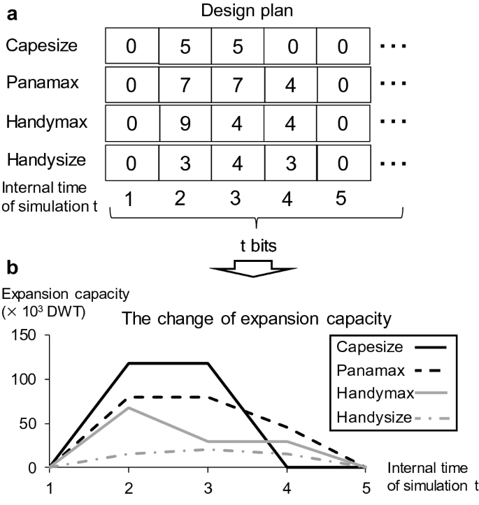

  

  Structure of design plan

  Table 2 Upper limitation of expansion capacity

  • Local search algorithm

  It is necessary that the local search algorithm searches neighboring solutions to the current solution in simulated annealing. We search neighbor solutions using five local search methods in this study. We select these methods at random:

  • (a) Swap: We select 2 bits on the design plan at random and interchange the values (Fig. 6a).

  • (b) Bit change: We select 1 bit on the design plan at random, and the values are changed at random (Fig. 6b).

  • (c) Insert: We select 1 bit and insert a point at random and the selected bit is inserted into that point (Fig. 6c).

  • (d) Reverse: We select 2 bits (start and end) on the design plan at random; the sequence of the internal bits is reversed (Fig. 6d).

  • (e) Infection: We select 1 bit on the design plan at random and the values of the surrounding 2 bits change to this value (Fig. 6e).

  Fig. 6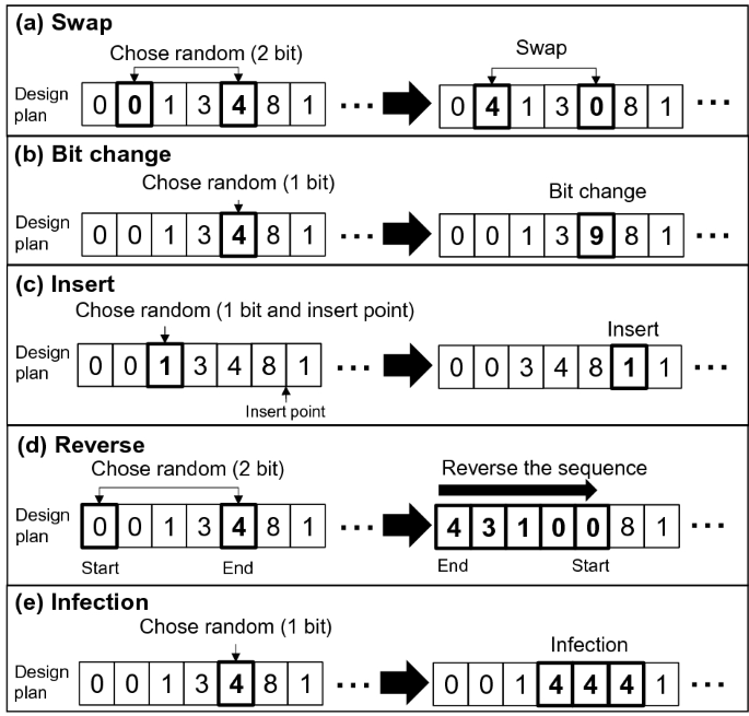

  

  Local search method

• 3. Evaluation

  The demand-forecasting simulation is conducted using the proposed demand-forecasting model in the lower problem. After that, the objective function is calculated using the result of the demand-forecasting simulation and Eq. 5. The details are discussed in Sect. 4.

• 4. Acceptable criterion

• 5. Transition

  The difference of profit Δp is determined using Eq. 13 in the new design plan. After that, we use the Metropolis criterion [26] as an acceptable criterion in Eq. 14. The Metropolis criterion is a criterion for determining whether to transition to the next state.

  $$\Delta p = \frac{{{\text{profit}}^{a} - {\text{profit}}^{a + 1} }}{{{\text{profit}}^{a} }},$$

  (13)
  $$Ap = \left\{ {\begin{array}{*{20}l} 1 & {{\text{if}}(\Delta p < 0)} \\ {\exp \left( {\frac{ - \Delta p}{T}} \right)} & {{\text{otherwise}}} \\ \end{array} ,} \right.$$

  (14)

  where profit is the total profit of the shipbuilding industry (USD), Δp is the difference in profit (–), T is the temperature (–), Ap is the acceptable probability (–), and a is the iteration time (–).

  If Δp improves (Δp becomes minus), Ap becomes “1” and the design plan Ep is updated to a new design plan. Otherwise, if Δp does not improve (Δp becomes plus), the design plan Ep is updated stochastically. In the case of a high temperature, the acceptable probability becomes high, and the design plan Ep easily moves toward a small profit. On the other hand, in the case of a low temperature, the acceptable probability becomes low, and the design plan Ep becomes difficult to move toward a small profit. Using this criterion, it can prevent falling into a local solution. The best design plan is saved and updated.

• 6. Cooling criterion

• 7. Cooling

  Cooling is conducted when the iteration time reaches the maximum in the cooling time k. This maximum cooling time is inputted by system users.

  In the cooling step, the temperature T^k+1 is calculated using Eq. (15). To keep the convergence of the solution, we avoid sharp drops of temperature in the simulated annealing algorithm. Therefore, in general, the temperature coefficient γ is set to over 0.8 and less than 1[32].

  $$T^{{_{{^{k + 1} }} }} = \gamma \times T^{{_{{^{k} }} }} ,$$

  (15)

  where T is the temperature (–), γ is the temperature coefficient (–), and k is the cooling time (–).

• 8. Stop criterion

  The algorithm is stopped when the cooling time reaches the maximum.

4 Overview of lower problem

4.1 Improvement of system dynamics model

In the lower problem, the demand-forecasting simulation is conducted using the proposed demand-forecasting model based on the simulation span, simulation scenarios (world GDP and cargo transportation distance scenarios), and initial values at the start of the simulation (bottoms, order books, construction capacity, and amount of ships under construction). The number of orders, amount of construction, ship price, etc., are then forecasted. The exogenous variables, simulation span, and initial values at the start of the simulation are set by the system user in advance. Based on the predicted values output from the SD model, the calculation of the objective function (Eq. 5) and the judgment of the constraint conditions (Eq. 11) are performed. It is possible to forecast construction capacity using the construction model of our previous study [24]. However, the demand-forecasting simulation is conducted using a design plan of construction capacity in the case of a construction capacity-control problem. Thus, the internal calculation of construction capacity by construction model is not conducted. As mentioned in Sect. 2.2, the construction model in the SD model has modeled characteristics of capacity expansion for shipbuilding based on actual results. By replacing the construction model with a design plan in optimization, we consider the fluctuation of the shipbuilding market when the construction capacity is expanded, which is different from the past characteristics.

It is necessary to develop the ship price prediction model and improve the demand-forecasting model to calculate the object functions and to check the constraint condition. Therefore, the demand-forecasting model is improved by developing the ship price-prediction model. This ship price model was integrated into the previous demand-forecasting model. The overview of the entire demand-forecasting model, integrated with the ship price-prediction model, is shown in Fig. 7. We define the backlog of the shipyards Bl, which means the stock rate of the order books. The backlog Bl is calculated using the order books, construction capacity, and period of facility expansion. The ship price is calculated using this backlog. The number of orders and the amount of construction, scrap, etc., are forecasted using this model by inputting only world GDP and cargo transportation distance.

Fig. 7

Overview of demand-forecasting model in this study

4.2 Development of ship the price-prediction model

Ship price fluctuates by internal influences in the shipbuilding market and external influences such as modification of international rules. Koyama et al. [10] and Nagatsuka et al. [11] focus on how the ship price fluctuates by internal influences on the shipbuilding market. They indicate that there is a strong correlation between the order books at the shipyards and the ship price. However, the data utilized in these studies are annual data and limited to shipbuilders in Japan. Accordingly, it is difficult to apply to a demand-forecasting model, because we target monthly demand forecasting and the worldwide market in this study. We refer to these studies [10, 11], and analyze the relation between order books at shipyards, construction capacity in shipyards, and the ship price based on latest market data. The ship price-prediction model is developed based on the analysis result. It is difficult to forecast the ship price fluctuation caused by the external influence. Therefore, we focus on the relation between ship price and the internal influences on the shipbuilding market.

The calculation equation for the backlog Bl and the ship price are defined in Eqs. 16 and 17

$${\text{Bl}}_{t} = \frac{{{\text{Ob}}_{t} }}{{f_{1} ({\text{Cp}}_{t} ,{\text{ep}})}},$$

(16)

$${\text{Sp}}_{t} = f_{2} ({\text{Bl}}_{t} ),$$

(17)

where Bl is the backlog at the shipyards (year), Ob the order books in the shipyards (DWT), f₁ the function to calculate annual construction capacity (–), Cp the construction capacity at the current month (DWT), and ep the period of facility expansion (month). Here, Sp is the ship price (index), f₂ is the function to calculate the ship price (–), and t is the internal time in the simulation (months).

The relation between the backlog and ship price is shown in Fig. 8. The ship price is forecasted using the characteristics developed below. It should be noted that “Ship price” denotes the average price for each ship size. The unit for the ship price is the index value (index), which is the definition used in the Clarkson Shipping Intelligence Network [33]. This ship price index is calculated in the lower problem. It converts to the average ship price (USD/DWT) using the relation in Fig. 9. The ship price (index) and average ship price (USD/DWT) consider all ship sizes (i.e., Capesize, Panamax, Handymax, and Handysize).

• 1. Rising period: The ship price increases as the backlog increases. The ship price increases rapidly when the backlog is between 1 and 3 years. However, the rate of the rising speed becomes gentler when the backlog is over 3 years.

• 2. Falling period: Ship price decreases as the backlog decreases. This is caused by the rapid expansion of construction capacity in the shipyards. The ship price decreases rapidly when the backlog is over 3.2 years. However, the ship price becomes constant when the backlog is between 3.2 years and 2.8 years. Additionally, if the backlog is less than 2.8 years, the ship price starts to fall.

• 3. Forced falling period: When the backlog at shipyards becomes nearly 1 year, the ship price is forced into falling by the shipyards to keep the amounts of order books considering a likely future recession. Additionally, when the ship price reaches the bottom, it enters the rising period (1).

Fig. 8

Relation between the backlog and ship price

Fig. 9

Relation between index and USD/DWT

These relations are defined using the following data from the Clarkson Shipping Intelligence Network [33]:

• 1. The amounts of order books (DWT) from 1998 to 2012.

• 2. The amounts of construction capacity (DWT) from 1998 to 2012; these are the analysis results in the previous study [24].

• 3. Ship price (Index) from 1998 to 2012.

4.3 Sub-model validation of ship price-prediction model

To confirm the validity of the proposed sub-model of ship price-prediction model, we conducted a demand-forecasting simulation from January 1998 to December 2012. The input data and outputs for the simulation are:

• The amounts of order books (DWT) from January 1998 to December 2012;

• The amounts of construction capacity (DWT) from January 1998 to December 2012.

The simulation results for the sub-model are shown in Fig. 10. In the figure, the solid line shows the simulation results, whereas the dotted line shows actual results. The sub-model for the ship price-prediction model reproduced the rapid increases and decrease in ship price from 2002 to 2005, from 2006 to 2008, and from 2008 to 2011. Thus, the proposed sub-model can reproduce the trends of the actual results; therefore, the validity of the proposed sub-model is confirmed.

Fig. 10

Simulation results of the ship price sub-model

4.4 Entire model validation

To confirm the validity of the entire proposed model, including the ship price-prediction model, we conducted a demand-forecasting simulation from January 1998 to December 2012. The input data for the simulation were as follows:

• Input scenario: from January 1998 to December 2012

  • 1. World GDP (actual data)

  • 2. Cargo transportation distance (actual data)

• Initial value:

  • 1. Bottoms: 2.65 × 10⁸ (DWT)

  • 2. Order books: 2.62 × 10⁷ (DWT)

  • 3. Construction capacity: 2.09 × 10⁶ (DWT)

  • 4. Ship amount under construction: 9.60 × 10⁶ (DWT)

The simulation results for the ship price and orders are shown in Fig. 11. In the figure, black solid lines show the simulation results while gray dotted lines show actual results. Clearly, the almost trend of ship price can be simulated well (Fig. 11 left). Additionally, the trend of orders can be simulated (Fig. 11 right). Focused on ship price forecasting results, the reproducibility of simulation is reduced. There is a difference between the simulation and actual results around 2002, from 2004 to 2005, and around 2008 compared with Fig. 10. This is the influence that the simulation result, especially the simulation results for orders, did not reproduce the short-term change with the proposed model. As a result, the difference between simulation results and actual results develops by this difference in accumulation.

Fig. 11

Simulation results for ship price and orders (1998–2012)

To confirm the number of months for which the proposed model reproduced the actual trend for price and ship orders, we conducted a correlation analysis between the simulation and actual results. The purpose of correlation analysis is to analyze how the output predicted values could reproduce the actual trends. We will verify the fineness of the model by correlation analysis. The moving average was taken against actual results for ship price and orders. The results are shown in Fig. 12. The solid gray lines in Fig. 11 show actual results by taking the moving average. The correlation coefficient for ship price was at a maximum (0.96 (–)) when the moving average period spanned 2 months. The correlation coefficient for the ship price decreases gradually when the moving average period is longer than 2 months. The correlation coefficient for orders was a maximum (0.89 (–)) when the moving average period spanned 6 months. Both the correlation coefficients for orders and ship price show high values. From these results, the proposed model can forecast the average trend for orders for 6 months and the average trend in ship price for 2 months. The moving average period set to 2 months is almost the same as without a moving average period. Therefore, the actual results without moving average (dotted lines), and the moving average of the actual results (gray solid lines) for ship price, are almost the same results as in Fig. 11.

Fig. 12

Results of correlation analysis on ship price and orders (1998–2012); (left: analysis result for ship price, right: analysis result for orders)

Based on the above discussion, the proposed entire model can reproduce the trends of the actual results; therefore, the validity of the entire proposed model is confirmed.

5 Case study

5.1 Past simulation

To consider the optimal timing and magnitude of the construction capacity expansion, we conducted optimization simulations. How the construction capacity expansion speed changes short-term and long-term and the effectiveness of the rapid construction capacity increase are verified by this simulation.

The simulation case, input scenario, initial value, constraint condition, and simulated annealing parameters are as follows:

• Simulation case

  Case 1: The simulation span is set from 2004 to 2011.

  Case 2: The simulation span is set from 2004 to 2020. The world GDP growth rate is set to 3.5% and the cargo transportation distance was assumed to be constant after 2016.

• Input scenario: from January 2004 to December 2015

  • 1. World GDP (actual data)

  • 2. Cargo transportation distance (actual data)

• Initial value:

  • 1. Bottoms: 3.02 × 10⁸ (DWT)

  • 2. Order books: 5.58 × 10⁷ (DWT)

  • 3. Construction capacity: 2.09 × 10⁶ (DWT)

  • 4. Ship amount under construction: 1.50 × 10⁷ (DWT)

• Constraint condition

  • 1. Constraint condition Mp is set to 1.0 × 10¹⁰ (USD)

• Simulated annealing parameters

  • 1. Initial temperature T₀: 0.15 (–)

  • 2. Iteration time It: 20 (times)

  • 3. Cooling time Ct: 150,000 (times)

  • 4. Temperature reduction coefficient γ: 0.999 (–)

The optimization results of the simulation for construction capacity and orders are shown in Fig. 13. For Case 1, the construction capacity optimization is executed until 2011 and construction capacity was assumed to be constant after 2013. The actual results are shown from 2004 to 2012. The construction capacity is expanded in conjunction with a rapid increase in orders from 2007 to 2008. Compared with the actual results, the trends of orders and construction capacity agree well. However, the number of orders remains at low levels after 2012 because of the excessive supply of ship bottoms.

Fig. 13

Optimization results for construction capacity and orders (2004–2020)

For Case 2, the construction capacity increases around 2007 and then becomes constant after 2010. Compared with Case 1, the construction capacity expansion starts quickly, and the maximum amount of construction capacity is 48.0% lower. The simulation results for orders are changed by this influence. For example, the number of orders decreases from 2007 to 2009 by a decrease in the construction capacity. After 2012, the shipbuilding industry takes constant orders. The start and end of the construction capacity expansion are almost identical with the start and end of the rapid increase in orders.

The optimization results for the profit of the shipbuilding industry are shown in Fig. 14. When we compare the actual result with Case 1, we see that the profit of the shipbuilding industry increases from 2007 to 2008 in conjunction with the orders. The trends of the profit agree well between the actual results and Case 1. The total profit for the shipbuilding industry is 4.05 × 10¹¹ (USD) in Case 1. However, the shipbuilding industry is in deficit around 2012 because of an excessive supply of ship bottoms. Similarly, the profits remain at a low level and continue to show a deficit after 2012. Therefore, the total profits decrease (3.37 × 10¹¹ (USD)) when the simulation span is from 2004 to 2020 in Case 1.

Fig. 14

Optimization results for profit (2004–2020)

On the other hand, the shipbuilding industry can acquire a sustainable profit in Case 2, because the construction capacity expansion is decreased and gentler. The total profit for the shipbuilding industry is 4.20 × 10¹¹ (USD). Comparing Cases 1 and 2, the shipbuilding industry makes more profits when the simulation span becomes long term.

The rapid expansion of the construction capacity is effective in obtaining a great profit in the 7 years from 2004 to 2011. However, the rapid expansion of construction capacity is not effective in the long term. Additionally, the oversupply of shipbuilding capacity does not occur if the expansion is stopped when the rapid increase of orders from 2006 to 2008 is over. From these results, we conclude that the current recession would not have occurred if the construction capacity expansion had been appropriately controlled.

5.2 Future simulation

To consider the optimal timing and amount of construction capacity reduction in the future, we performed further optimization simulations. The input scenario, initial values, and simulation cases are described below. The simulated annealing parameters are the same as in Sect. 5.1, and the constraint condition Mp is not considered in the simulation because it is difficult to satisfy the constraint condition based on 2013.

• Simulation case

  Case 3: Construction capacity is assumed constant from 2013 to 2030.

  Case 4: Considering construction capacity reduction

• Input scenario: from January 2013 to December 2030

  • 1. World GDP (actual data until 2015)

  • 2. World GDP growth rate: 3.5% after 2016

  • 3. Cargo transportation distance: actual data until 2015 and assumed constant after 2016

• Initial value:

  • 1. Bottoms: 6.92 × 10⁸ (DWT)

  • 2. Order books: 1.27 × 10⁸(DWT).

  • 3. Construction capacity: 1.14 × 10⁷ (DWT).

  • 4. Ship amount under construction: 4.84 × 10⁷ (DWT).

The optimization results of the construction capacity are shown in Fig. 15 left. The maximum construction capacity continues constantly until 2030 in Case 3. In Case 4, the construction capacity continues to decrease until 2017, when it becomes almost constant. Compared with Case 3, the construction capacity decreases by 59.6% in Case 4. The optimization results for profits are changed by this influence.

Fig. 15

Optimization results for construction capacity and profit (2013–2030)

The optimization results for the profit of the shipbuilding industry are shown in Fig. 15, right. The difference in profits was approximately 9 times between Case 3 (0.92 × 10¹⁰ (USD)) and Case 4 (8.40 × 10¹⁰ (USD)). The total profits increase by ship construction capacity decrease. In Case 3, the shipbuilding industry is in a deficit from 2015 to 2019, and the profits are changed at low levels after 2020. In Case 4, the shipbuilding industry is in a deficit from 2015 to 2018, and the profits continuously increase after 2023. The comparison results of Case 3 and Case 4 are summarized below:

• The shipbuilding market recovers faster, and the deficit is smaller in Case 4 compared with Case 3.

• There is a big difference in profits after 2023 between Case 3 and Case 4, which is due to the increase in ship prices resulting from a decrease in construction capacity.

Thus, the more shipbuilding capacity is reduced, the more profit the shipbuilding industry makes.

From the results in Sects. 5.1 and 5.2, we can consider the optimal timing and magnitude of construction capacity expansion or reduction influence on the shipbuilding market using the proposed system.

5.3 Analysis of the impact of changing problem settings

5.3.1 Change of configuration problems

For Sects. 5.1 and 5.2, the optimization simulation was executed from the shipbuilding industry aspects. However, the shipping industry aspects are not considered in these simulations. In this section, we include the shipping industry aspects and consider how this changes the shipbuilding demand-forecasting simulation. Furthermore, the expansion of the construction capacity is replaced with the construction model by the system dynamics model, and the difference from the optimization result is considered.

Incidentally, the ship running distance is defined and used to forecast shipbuilding demand. This ship running distance shows the sailing distance of ships in 1 month and indicates the condition of the shipping market. The ship running distance is calculated based on the amount of cargo transportation (tons-miles) and ship bottoms.

The relation between the ship running distance and the orders for new ships is shown in Fig. 16. As shown in the figure, the number of orders increases as the ship runningdistance gradually increases in the ordinary condition. On the other hand, when the ship running distance continues to increase, the operation of ships reaches a critical limit. In such a case, the number of orders increases rapidly. Thus, the amounts of transportation demand and ship supply become imbalanced because the ship bottoms are insufficient. Therefore, the number of orders increases rapidly, and it is necessary to consider the ship running distance and adjust the ship bottoms to realize stable transportation in the shipping industry.

Fig. 16

Relation between ship running distance and total order rate

We add Eq. (18) below, considering the ship running distance as a constraint condition. Cp is the critical limit of the ship’s operation. In summary, the ship bottoms become sufficient by this constraint condition.

$${\text{SRD}}_{t} \le {\text{Cp,}}$$

(18)

where SRD is the ship running distance in 1 month (mile), Cp the critical limit of ship running distance for ship operation (mile), and t the internal time in the simulation (months).

5.3.2 Simulation result

To consider the influence of the configuration problem, we conducted optimization simulations. The simulation cases and constraint conditions were as follows. The input scenarios, initial values, and simulated annealing parameters are the same as in Sect. 5.1.

• Simulation case

  Case 5:The simulation span is set from 2004 to 2020. The world GDP growth rate is set to 3.5%, and the cargo transportation distance is assumed constant after 2016.

  Case 6: The simulation span is set from 2004 to 2020. Capacity expansion was executed based on the construction model in the system dynamics model (Fig. 7). The scenario of the world GDP growth and the cargo transportation distance is the same with Case 5. Optimization calculation is not conducted; therefore, a constraint condition is not applied.

• Constraint condition

  • 1. Constraint condition Cp is set to 2250.00 (miles).

  • 2. Constraint condition MP in Eq. 11 is not set.

The simulation results for the construction capacity are shown in Fig. 17 left. Case 2 is the optimization results that only consider shipbuilding aspects as in Sect. 5.1. In Case 5, the construction capacity results are expanded from 2004 to 2006, and the construction capacity expansion becomes constant after 2007. The construction capacity increases gently after 2010. The shipbuilding capacity increases at an earlier time of the simulation compared with Case 2. The capacity-expansion speed is slower than in Case 2. The maximum construction capacity is almost the same as for Case 2. Conversely, construction capacity expansion results in Case 6 became almost the same trend as the actual result. The construction capacity expansion stopped around 2011 and resumed around 2012 in Case 6. The maximum construction capacity is about the same as the actual results because the construction model in the system dynamics model has modeled the actual shipbuilding capacity based on the actual results. As a result, the transition of the construction model after 2013 will be constant.

Fig. 17

Optimization results for construction capacity and orders (2004–2020)

The simulation results for orders are shown in Fig. 17 right. For Case 5, more ships are added into the ship bottoms from 2004 to 2005 by the shipbuilding capacity expansion. As a result, the shipping company can use more ships than the actual result in 2008. Therefore, the rapid increase in orders is significantly suppressed. In Case 6, the simulation results on orders the same as the actual tendency became almost equal from 2004 to 2012. The amount of ship bottoms becomes insufficient; a rapid increase in orders occurs.

The optimization results for the ship running distance are shown in Fig. 18 left. The constraint condition Cp is satisfied in Case 5. This is because the amounts of ship construction increase from 2004 to 2005 by an early construction capacity expansion. By this influence, the tightness of ship bottoms is relieved compared with the actual result and Case 2. On the other hand, the constraint condition is not satisfied from 2007 to 2008 in the actual results and Case 2, Case 6.

Fig. 18

Optimization results for ship running distance and profit (2004–2020)

The optimization results for profit are shown in Fig. 18, right. The total profit for the shipbuilding industry is 3.97 × 10¹¹ (USD) in Case 5. However, the total profits in Case 5 are 5.5% lower than for Case 2. Total shipbuilding profits are decreased because the tightness of ship bottoms is relieved.

Case 6 has the same tendency as the actual results and can secure a large profit in the short term. However, it is in deficit in 2011–2013 and 2016–2018, and it has not been able to secure sufficient profit since 2011. The total profit for the shipbuilding industry is 2.55 × 10¹¹ (USD) in Case 6.

From the above, the simulation results are significantly different between the case considering only shipbuilding industry aspects and the case considering both shipbuilding and shipping industry aspects. Additionally, we compared the simulation results using the system dynamics model and optimization and considered the differences. As a result, the optimization expansion scenario can be obtained even if the simulation conditions are changed. Thus, it can be applied to various problems depending on the setting of the system user.

5.4 Discussion

In this section, we consider the simulation results of Sects. 5.1–5.3. Table 3 summarizes the objective of simulation for each simulation case of Sects. 5.1–5.3.

Table 3 Objective of each simulation case

In Sect. 5.1, Case 1 and Case 2 were compared, and the changes in shipbuilding capacity expansion due to different simulation periods were compared. As a result, the actual results and Case 1 show almost the same construction capacity expansion, and the shipbuilding market is to pursue short-term profits. Conversely, Case 2 has secured long-term profits by stopping the expansion of construction capacity in 2010. As shown in Case 2, a long-term analysis of the impact of capacity expansion is necessary from 2010 to stop the expansion of construction capacity. A forecast model for the shipbuilding market is considered essential to make such decisions.

In Sect. 5.2, we examined the impacts of shipbuilding construction capacity reduction to recover the market. As a result, the shipbuilding market will be able to secure profits by sharply reducing construction capacity. From this result, it is considered unhealthy in the entire shipbuilding market by subsidy or financial support from the government. It is necessary to formulate rules for shipyard support.

In Sect. 5.3, we analyzed the characteristics of the expansion of the construction capacity to analyze the impact of changing the problem settings. Case 5 is a simulation that prevents a shortage of vessels in shipping by not causing vessels' order explosion. In this case, it is necessary to expand the shipbuilding capacity at an early stage and slowly. In Case 6, a simulation was also performed when the construction model was replaced in the system dynamics model in the previous study. Since Case 6 models the expansion of shipbuilding capacity in actual results, simulation results become the same as actual results until 2012. In addition, there is no significant difference between the results of Case 6 and the results of Case 1 until 2011; the construction capacity and order quantity are almost the same. From these results, the system dynamics model (Case 6) and Case 1 are expanding the construction in pursuit of short-term profits.

Considering the above results comprehensively, we notice that Case 2 is considered a scenario in which profits can be obtained even after 2012 while securing profits in the shipbuilding market. To realize this scenario, it is necessary to make a different decision from the actual expansion of construction capacity. In addition, through these discussions, it was shown that the proposed method and model could be used to study scenarios that consider the sustainable development of the shipbuilding market. The proposed model and system can be used by international organizations such as OECD wp6 and the governments of shipbuilding countries for policy planning.

As mentioned in Sect. 2.4, we focused on the entire shipbuilding capacity and formulated the shipbuilding adjustment problem as an optimization problem. From this point of view in the formulation, it is difficult to consider the market fluctuation caused by differences in the strategy of each country. Similarly, it is also difficult to consider competition between shipyards and the difference in strategy. On the other hand, as pioneer research, Shin et al. [17] developed an empirical model of national competition in the shipbuilding industry using the Cournot oligopoly with Choquet Expected Utility (CEU) theory, as mentioned in Sect. 1.2. By incorporating the model of this research and upgrading the model in consideration of the difference in ship production costs, it may be possible to consider the optimal shipbuilding strategy for shipyards and the country. Additionally, maritime industry consists not only of shipyards, but also ship owners, operators, shippers, the ship equipment industry, etc., and it is also important to consider these stakeholders from a whole maritime industry aspect. In this study, we executed a simulation that prevented a shortage of vessels in shipping by avoiding an order explosion for vessels in Case 5. However, the logistic service and freight rate were not considered in this study. To consider the many stakeholders, the method of systems engineering was considered to be effective. In recent years, Hiekata et al. [23] developed a system to support the introduction of Internet of things (IoT) technologies in the maritime industry by considering the relations between stakeholders using the stake holder value network [34] and object-process methodology [35]. When using systems engineering techniques, it is necessary to improve the model to support multiple stakeholders in the maritime industry.

6 Conclusion

In this study, we developed a simulation system to consider shipbuilding capacity adjustment for the shipbuilding industry and discussed optimal shipbuilding capacity-adjustment scenarios using the proposed system. The key findings are as follows:

• 1. We developed a simulation system to consider the shipbuilding capacity adjustment using an optimization method. We described the proposed demand-forecasting model, provided an overview of the system, and formulated it as an optimization problem.

• 2. To predict ship prices, we examined causal relations between order books in shipyards, construction capacity, and ship price, defining a new ship price-prediction model. Additionally, the ship price-prediction model was integrated into the previous demand-forecasting model.

• 3. To confirm the validity of the proposed ship price-prediction model and the entire demand-forecasting model, we performed demand-forecasting simulations.

• 4. To consider the optimal timing and quantity of construction capacity expansion or reduction, we conducted optimization simulations. We showed that the shipbuilding industry grew continuously by proper control of construction capacity expansion or reduction. The effectiveness of the proposed system was also shown by the simulation.

• 5. To confirm the effectiveness of the proposed system, we executed a simulation in different scenario settings. The characteristics of the simulation results were analyzed by comparing the case considering only shipbuilding industry aspects, the case considering both shipbuilding and shipping industry aspects, and the case using a construction model in a previous study.

We focused on the imbalances of supply and demand of the shipbuilding industry and developed a shipbuilding capacity-adjustment system. Therefore, in future work, we will improve the system so it will be able to consider optimal strategy based on competition between countries or shipyards. Additionally, the target industry of the shipbuilding capacity-adjustment system was only the shipbuilding industry. Therefore, it was difficult to consider the influence of some stakeholders, such as the shipping industry and the ship equipment industry. We will develop a system that takes the influence of these stakeholders into account. Furthermore, the proposed model predicts the amount of sea cargo movement using GDP and cargo transportation distance. However, it is difficult to predict these values because of some uncertainty involved. In future work, we are considering handling these uncertainties.

References

Organisation for Economic Cooperation and Development (OECD) (2017) Imbalances in the shipbuilding industry and assessment of policy responses, C/WP6(2016)6/final
Taylor AJ (1975) The dynamics of supply and demand in shipping. Dynamica 2:62–71
Nielsen KS, Kristensen NE, Bastiansen E, Skytte P (1982) Forecasting the market for ships. Long Range Plan 15:70–75
Japan Maritime Research Institute SD Study Group (1978) SD model of maritime transportation and shipbuilding. Japan Maritime Research Institute the Bulletin, 142 (In Japanese)
Sakalayen QMH, Duru O, Hirata E (2021) An econophysics approach to forecast bulk shipbuilding orderbook: an application of Newton’s law of gravitation. Marit Bus Rev 6(3):234–255
Beenstock M (1985) A theory of ship prices. Marit Policy Manag 12:215–225
Beenstock M, Vergottis A (1989) An econometric model of the world shipping market for dry cargo, freight and shipping. Appl Econ 21:339–356
Beenstock M, Vergottis A (1989) An econometric model of the world tanker market. JTEP 23:263–280
Jin D (1993) Supply and demand of new oil tankers. Marit Policy Manag 20(3):215–227
Koyama T, Watanabe I, Hattori K (1993) Analysis on order books at shipyards in Japan and system dynamics model. Jpn Marit Res Inst Bull 93–154:1–73 (In Japanese)
Nagatsuka S, Nakahara T (2003) Analysis and transition on the change of newbuilding price of ships. Jpn Marit Res Inst Bull 2003–236:1–55 (In Japanese)
Gourdon K (2019) An analysis of market-distorting factors in shipbuilding: the Role of Government interventions, OECD Science, technology and industry policy papers, vol 67. OECD Publishing, Paris
Won DH (2010) A study of Korean shipbuilders' strategy for sustainable growth. Diss. Massachusetts Institute of Technology
Paul WS (1995) Marketing strategy for merchant shipbuilders. Soc Nav Archit Mar Eng 26:1–14
Jun WJ, Ying W, Gi TY (2016) Ship safety policy recommendations for Korea: application of system dynamics. Asian J Shipp Logist 32(2):73–79
Lee T (2004) The dynamics of the oil tanker industry. Diss. Massachusetts Institute of Technology
Shin J, Lim Y-M (2014) An empirical model of changing global competition in the shipbuilding industry. Marit Policy Manag 1:515–527
Paul WS (2017) Competition and subsidy in commercial shipbuilding, Diss. Newcastle University
Elmahdi A, Malano H, Etchells T, Khan S (2005) System dynamics optimisation approach to irrigation demand management. In: MODSIM 2005 international congress on modelling and simulation, modelling and simulation Society of Australia and New Zealand, pp 196–202
McSharry P (2004) Optimization of system dynamics models using genetic algorithms, submitted to World Bank Report
Wada Y, Hamada K, Hirata N (2017) A study on the application of system dynamics model for demand forecasting of ships. Conference Proceedings of the Japan Society of Naval Architects and Ocean Engineers, 24, Annual Spring Meeting, 2017 (In Japanese)
Wada Y, Hamada K, Hirata N (2017) A study on the improvement and application of system dynamics model for demand forecasting of ships. International conference on computer applications in shipbuilding 2017, 1, pp 51–60
Hiekata K, Wanaka S, Mitsuyuki T et al (2020) Systems analysis for deployment of internet of things (IoT) in the maritime industry. J Mar Sci Technol 26:459–469
Wada Y, Hamada K, Hirata N, Seki K, Yamada S (2018) A system dynamics model for shipbuilding demand forecasting. J Mar Sci Technol 23(2):236–252
Meadows DH, Meadows DL, Randers J, Behrens WW III (1972) The limits to growth. Universe Books, Cambridge
Kirkpatrick S, Galatt DC, Vecchi MP (1983) Optimization by simulated annealing. Science 220(4598):671–680
Ministry of land, infrastructure transport and tourism (2016) Foreign exchange tolerance of Japanese shipbuilding industry analysis of shipbuilding cost structure (In Japanese)
Ministry of Economy, Trade and Industry (2015) Current status and problems of steel industry (mainly on blast furnaces) (In Japanese)
The Shipbuilders’ Association of Japan (2008) SAJ news, 112 (In Japanese)
Shipbuilding text research group (2001) Basic knowledge of merchant ship design, Seizando, Tokyo (In Japanese)
The Shipbuilders’ Association of Japan (2009) The shipbuilders association of Japan news, 124 (In Japanese)
Miki M, Ueda Y, Hiroyasu T (2008) Effectiveness of simulated annealing with advanced adaptive neighborhood for a real optimization problem—application to gain flattening filter. IPSJ J 49(10):3567–3575 (In Japanese)
Clarksons, Clarksons Shipping Intelligence Network. http://www.clarksons.net. Accessed 4 Oct 2013
Cameron B, Crawley E, Loureiro G, Rebentisch E (2008) Value flow mapping: using networks to inform stakeholder analysis. Acta Astronaut 62:324–333
Dori D (2002) Object-process methodology: a holistic systems paradigm. Springer, Berlin
Acknowledgements
This work was supported by JSPS KAKENHI Grant number JP21K04501, JP20H00286 and JP20H02371.
Author information
Authors and Affiliations
Corresponding author
Additional information
Publisher's Note
Springer Nature remains neutral with regard to jurisdictional claims in published maps and institutional affiliations.
Rights and permissions
This article is published under an open access license. Please check the 'Copyright Information' section either on this page or in the PDF for details of this license and what re-use is permitted. If your intended use exceeds what is permitted by the license or if you are unable to locate the licence and re-use information, please contact the Rights and Permissions team.
About this article
Cite this article
Wada, Y., Hamada, K. & Hirata, N. Shipbuilding capacity optimization using shipbuilding demand forecasting model. J Mar Sci Technol 27, 522–540 (2022). https://doi.org/10.1007/s00773-021-00852-8
Received:
Accepted:
Published:
Issue Date:
DOI: https://doi.org/10.1007/s00773-021-00852-8