Various dimensional colour image encryption based on non-overlapping block-level diffusion operation

Abstract

This paper proposes a colour image encryption scheme to encrypt colour images of arbitrary sizes. In this scheme, a fixed block size (3 × 8) based block-level diffusion operation is performed to encrypt arbitrary sized images. The proposed technique overcomes the limitation of performing block-level diffusion operations in arbitrary sized images. This method first performs bit-plane decomposition and concatenation operation on the three components (blue, green, and red) of the colour image. Second it performs row and column shuffling operation using the Logistic-Sine System. Then the proposed scheme executes block division and fixed block-level diffusion (exclusive-OR) operation using the key image generated by the Piece-wise Linear Chaotic Map. At last, the cipher image is generated by combining the diffused blocks. In addition, the SHA-256 hashing on plain image is used to make chaotic sequences unique in each encryption process and to protect the ciphertext against the known-plaintext attack and the chosen-plaintext attack. Simulation results and various parameter analysis demonstrate the algorithm’s best performance in image encryption and various common attacks.

1 Introduction

Nowadays, lots of image data are being communicated through the internet. Security of those image data is of utmost importance. To achieve this, various conventional encryption techniques (Coppersmith 1994; Pub 2001) are used. But these techniques are not provided an efficient level of security to secure images because of high correlation among adjacent pixels and the large data requirement in images (Gao et al. 2006; Gupta et al. 2016).

To solve the above problem, it is important to focus on methods that satisfy the need of efficient security to images. Chaos system based algorithms have gathered much attention of a large number of researches in recent years. There are several inherent features of chaos systems such as sensitivity to initial values, randomness, ergodicity, determinacy, and non-periodicity. It is because of these features that the chaos based encryption system is found more reliable and suitable for high-security encryption (Guesmi et al. 2016a). Researchers have developed various chaos based encryption systems.

In 2012, Wei et al. (2012) suggested a combined DNA and hyper-chaotic map based colour image encryption technique. In this technique, authors used equal sized blocks (4 × 4) to perform the block diffusion operation. In 2014, Liu et al. (2014) developed an image encryption technique using chaos. In this scheme, authors used fixed sized blocks (8 × 8) to perform block diffusion operation. In 2016, Belazi et al. (2016) suggested a substitution-permutation based image encryption technique using chaos. In this technique also the block (fixed size 8 × 8) based operations are executed.

In all the above techniques (Wei et al. 2012; Liu et al. 2014; Belazi et al. 2016), one common problem is that the fixed sized blocks for diffusion operation is only applicable for fixed sized images. That means the image size should be exactly divisible by the block size. This problem can be overcome by the proposed technique. In this technique, the block of size (3 × 8) is used in block diffusion operation to encrypt arbitrary size images.

This paper contributes the followings.

• The chaotic map “Piece-wise Linear Chaotic Map (PWLCM)” is utilized to generate a block of size (3 × 8) to perform the block diffusion operation. The generated block is termed as key image.

• The chaotic map “Logistic-Sine System (LSS)” is utilized to perform the row-column shuffling operation.

• The hash algorithm “SHA-256” is utilized to generate hash based keys.

The rest part of the paper is as follows. Section 2 introduces all the chaotic maps used in this scheme. Section 3 illustrates the proposed method. Section 4 throws light on the result and security analysis with different images. Lastly the conclusion remarks in Sect. 5.

2 Preliminaries

2.1 PWLCM system

As compared to Logistic map, the PWLCM system is less sensitive towards external perturbations. Due to this characteristic, in recent encryption algorithms, PWLCM system is used (Li et al. 2005; Wang and Yang 2012; Patro and Acharya 2018). The mathematical expression for PWLCM system is

$$p_{n + 1} = \left\{ {\begin{array}{*{20}l} {\frac{{p_{n} }}{u}} \hfill & {\quad if \quad 0 \le p_{n} < u} \hfill \\ {\frac{{p_{n} - u}}{0.5 - u}} \hfill & {\quad if \quad u \le p_{n} < 0.5} \hfill \\ {\left( {1 - p_{n} } \right)} \hfill & {\quad if \quad 0.5 \le p_{n} < 1} \hfill \\ \end{array} } \right.$$

(1)

where, $p_{n}$ (termed as “initial value”) and $u$ (termed as “system parameter”) lies in the range (0, 1) and (0, 0.5), respectively.

2.2 L SS map

The LSS map is derived by integrating two existing 1D chaotic maps such as Sine and Logistic. The resulting 1D chaotic system is found to have excellent chaotic properties with improved uniform distribution variant density function. Individually the 1D chaotic maps; Sine and Logistic do not have a uniform distribution, but their combination shows a simple and highly reliable system. The mathematical expression for LSS map is as follows (Zhou et al. 2014).

$$q_{n + 1} = \left( {v \times q_{n} \left( {1 - q_{n} } \right) + \left( {4 - v} \right)\sin \left( {\pi q_{n} } \right)/4} \right) mod 1$$

(2)

where, $q_{n}$ (termed as “initial value”) and $v$ termed as “system parameter”) lies in the range (0, 1) and (0, 4), respectively.

2.3 Secure hash algorithm

Secure Hash Algorithm (also referred as a file check function) has come up to meet the rising cyber attacks of the 21st century. The family of secure hash algorithms is SHA-0, 1, 2 and 3, where as SHA-256 hash algorithm is a member of SHA-2. SHA-256 algorithm sets up a uniquely exclusive 256-bit hash of fixed size. Hash function generates hash as a simplex criterion which means a hash cannot be decrypted back thus making it important for applications like digital signatures, encryption key management, password logins, etc. In this paper, SHA-256 is used to generate the keys of the algorithm.

3 Proposed methodology

This section presents a proposed colour image encryption algorithm based on non-overlapping block-level diffusion operation. Figure 1 shows the image encryption system. Followings are the steps of image encryption system.

Fig. 1

Colour image encryption system

• 1. Input an $M_{CI} \times N_{CI}$ sized colour image $I_{CI}$.

• 2. Generate hash value of 256-bits of image $I_{CI}$ using the “Secure Hash Algorithm SHA-256″. Then generate 64-hex value from the hash output of 256-bits. The hex value is represented as,

  $$hs = hs_{1} ,hs_{2} ,hs_{3} , \ldots ,hs_{63} ,hs_{64} \;and\;each\;hs_{i} \left( {1 \le i \le 64} \right)is\;expressed\;as\;\left\{ {hs_{i,0} , hs_{i,1 ,} hs_{i,2 ,} hs_{i,3} } \right\}$$

• 3. Separate Blue ($B_{CI}$), Green ($G_{CI}$), and Red ($R_{CI}$) components of the image $I_{CI}$.

• 4. Generate bit-planes of $R_{CI}$, $G_{CI}$, and $B_{CI}$ using “Binary Bit-plane Decomposition” technique by,

  $$\left\{ {\begin{array}{*{20}c} {R1_{CI} = bitget\left( {R_{CI} ,1} \right)} \\ {R2_{CI} = bitget\left( {R_{CI} ,2} \right)} \\ {\begin{array}{*{20}c} {R3_{CI} = bitget\left( {R_{CI} ,3} \right)} \\ {R4_{CI} = bitget\left( {R_{CI} ,4} \right)} \\ {\begin{array}{*{20}c} {R5_{CI} = bitget\left( {R_{CI} ,5} \right)} \\ {R6_{CI} = bitget\left( {R_{CI} ,6} \right)} \\ {\begin{array}{*{20}c} {R7_{CI} = bitget\left( {R_{CI} ,7} \right)} \\ {R8_{CI} = bitget\left( {R_{CI} ,8} \right)} \\ \end{array} } \\ \end{array} } \\ \end{array} } \\ \end{array} } \right.$$

  where, $\left( {R1_{CI} ,R2_{CI} ,R3_{CI} ,R4_{CI} ,R5_{CI} ,R6_{CI} , R7_{CI} , R8_{CI} } \right)$ are the bit-planes of $R_{CI}$ only. The function “bitget” generates the image bit-planes.

  Similarly, generate bit-planes of $G_{CI}$ and $B_{CI}$ using the same “Binary Bit-plane Decomposition” technique. The generated bit-planes of $G_{CI}$ and $B_{CI}$ are $\left( {G1_{CI} ,G2_{CI} ,G3_{CI} ,G4_{CI} ,G5_{CI} ,G6_{CI} , G7_{CI} , G8_{CI} } \right)$ and $\left( {B1_{CI} ,B2_{CI} ,B3_{CI} ,B4_{CI} ,B5_{CI} ,B6_{CI} , B7_{CI} ,B8_{CI} } \right)$, respectively.

• 5. Horizontally concatenate the $R_{CI}$ component bit-planes $\left( {R1_{CI} ,R2_{CI} ,R3_{CI} ,R4_{CI} ,R5_{CI} ,R6_{CI} , R7_{CI} , R8_{CI} } \right)$ by,

  $$R_{horz} = horzcat\left( {R1_{CI} ,R2_{CI} ,R3_{CI} ,R4_{CI} ,R5_{CI} ,R6_{CI} , R7_{CI} , R8_{CI} } \right)$$

  where, $R_{horz}$ is the horizontally concatenated output of size $M_{CI} \times 8N_{CI}$. The function “horzcat” horizontally concatenates the matrices.

  Similarly, horizontal concatenate the $G_{CI}$ and $B_{CI}$ component bit-planes to generate $G_{horz}$ and $B_{horz}$ of size $M_{CI} \times 8N_{CI}$, respectively.

• 6. Vertically concatenate $R_{horz}$, $G_{horz}$, and $B_{horz}$ by,

  $$RGB_{vert} = vertcat\left( {R_{horz} , G_{horz} , B_{horz} } \right)$$

  In the above expression, the concatenated output is denoted as $RGB_{vert}$ of size $3M_{CI} \times 8N_{CI}$. The function “vertcat” vertically concatenates the matrices.

• 7. Generate the key parameters of Logistic-Sine System-1.

  $$\left\{ {\begin{array}{*{20}l} {r1 = r + \left( {\left( {\frac{{mod\left( {\left( {hs_{1} + hs_{2} + \cdots + hs_{11} } \right),256} \right)}}{{2^{9} }}} \right) \times 0.1} \right)} \hfill \\ {x1\left( 1 \right) = x\left( 1 \right) + \left( {\left( {\frac{{mod\left( {\left( {hs_{12} + hs_{13} + \cdots + hs_{22} } \right),256} \right)}}{{2^{9} }}} \right) \times 0.1} \right)} \hfill \\ \end{array} } \right.$$

  (3)

  where, $x\left( 1 \right)$ (termed as “initial value”) and $r$ (termed as “system parameter”) are the original key parameters and $x1\left( 1 \right)$ (termed as “initial value”) and $r1$ (termed as “system parameter”) are the generated key parameters.

• 8. Generate a sequence $x1$ by iterating the Eq. (2) $3M_{CI}$ times.

• 9. Generate index values of the chaotic sequence $x1$ by,

  $$\left( {x1st,x1inx} \right) = sort\left( {x1} \right)$$

  where, $x1st$ is the sorted sequence of $x1$ and $x1inx$ is the sequence which stores the corresponding indexed values of $x1st$.

• 10. Using the indexed values of $x1inx$, execute the row shuffling operation. Let $RS_{CI}$ is the output of the row shuffling operation.

• 11. Generate the key parameters of Logistic-Sine System-2.

  $$\left\{ {\begin{array}{*{20}l} {r2 = r + \left( {\left( {\frac{{mod\left( {\left( {hs_{23} + hs_{24} + \cdots + hs_{33} } \right),256} \right)}}{{2^{9} }}} \right) \times 0.1} \right)} \hfill \\ {x2\left( 1 \right) = x\left( 1 \right) + \left( {\left( {\frac{{mod\left( {\left( {hs_{34} + hs_{35} + \cdots + hs_{44} } \right),256} \right)}}{{2^{9} }}} \right) \times 0.1} \right)} \hfill \\ \end{array} } \right.$$

  (4)

  where, $x\left( 1 \right)$ (termed as “initial value”) and $r$ (termed as “system parameter”) are the original key parameters and $x2\left( 1 \right)$ (termed as “initial value”) and $r2$ (termed as “system parameter”) are the generated key parameters.

• 12. Generate a sequence $x2$ by iterating the Eq. (2) $8N_{CI}$ times.

• 13. Generate index values of the chaotic sequence $x2$ by,

  $$\left( {x2st,x2inx} \right) = sort\left( {x2} \right)$$

  where, $x2st$ is the sorted sequence of $x2$ and $x2inx$ is the sequence which stores the corresponding indexed values of $x2st$.

• 14. Using the indexed values of $x2inx$, execute the column shuffling operation of $RS_{CI}$. Let $CS_{CI}$ is the output of the column shuffling operation.

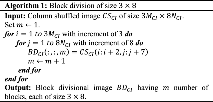
• 15. Divide $CS_{CI}$ into blocks of size $3 \times 8$. The reason for using block division of size $3 \times 8$ is that, for any sized colour image, it has three colour components and eight bit-planes. Hence the block size is $3 \times 8$. The block divisional output is denoted as $BD_{CI}$. Algorithm 1 shows the process of block division operation.

  

• 16. Generate the key parameters of PWLCM system.

  $$\left\{ {\begin{array}{*{20}l} {mue = mue1 + \left( {\left( {\frac{{mod\left( {\left( {hs_{45} + hs_{46} + \cdots + hs_{54} } \right),256} \right)}}{{2^{9} }}} \right) \times 0.1} \right)} \hfill \\ {y1\left( 1 \right) = y\left( 1 \right) + \left( {\left( {\frac{{mod\left( {\left( {hs_{55} + hs_{56} + \cdots + hs_{64} } \right),256} \right)}}{{2^{9} }}} \right) \times 0.1} \right)} \hfill \\ \end{array} } \right.$$

  (5)

  where, $y\left( 1 \right)$ (termed as “initial value”) and $mue1$ (termed as “system parameter”) are the original key parameters and $y1\left( 1 \right)$ (termed as “initial value”) and $mue$ (termed as “system parameter”) are the generated key parameters.

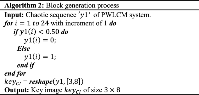
• 17. Generate a sequence $y1$ by iterating the Eq. (1) 24 times.

• 18. Generate a block of size $3 \times 8$ using the sequence $y1$. The generated block is also known as key image of the algorithm. Algorithm 2 shows the block generation process.

  

• 19. Execute diffusion operation (exclusive-OR) in block level between block components of ${\text{BD}}_{\text{CI}}$ and the key image ${\text{key}}_{\text{CI}}$. First execute diffusion operation between the first block component of ${\text{BD}}_{\text{CI}}$ and the key image ${\text{key}}_{\text{CI}}$. Second execute XOR operation between the output of the first XOR operation and the second block component of ${\text{BD}}_{\text{CI}}$. Third execute XOR operation between the output of the second XOR operation and the third block component of ${\text{BD}}_{\text{CI}}$. Likewise diffuse all the block components of ${\text{BD}}_{\text{CI}}$.

• 20. Combine all the diffused block components to generate a block diffused image ${\text{CBD}}_{\text{CI}}$.

• 21. Separate the three sections of bit planes. Each section contains eight bit planes. The three sections of bits planes are denoted as ${\text{CCR}}_{\text{CI}}$, ${\text{CCG}}_{\text{CI}}$, and ${\text{CCB}}_{\text{CI}}$. The separation process is as follows.

  $$\left\{ {\begin{array}{*{20}l} {CCR_{CI} = CBD_{CI} \left( {1:M_{CI} ,:} \right)} \hfill \\ {CCG_{CI} = CBD_{CI} \left( {M_{CI} + 1:2 \times M_{CI} ,:} \right)} \hfill \\ {CCB_{CI} = CBD_{CI} \left( {2 \times M_{CI} + 1:3 \times M_{CI} ,:} \right)} \hfill \\ \end{array} } \right.$$

• 22. Separate eight bit planes of each of the sections ${\text{CCR}}_{\text{CI}}$, ${\text{CCG}}_{\text{CI}}$, and ${\text{CCB}}_{\text{CI}}$. The bit plane separation process of ${\text{CCR}}_{\text{CI}}$ is as follows.

  $$\left\{ \begin{aligned} CCR1_{CI} = CCR_{CI} \left( {:,1:N_{CI} } \right) \hfill \\ CCR2_{CI} = CCR_{CI} \left( {:,N_{CI} + 1:2 \times N_{CI} } \right) \hfill \\ CCR3_{CI} = CCR_{CI} \left( {:,2 \times N_{CI} + 1:3 \times N_{CI} } \right) \hfill \\ CCR4_{CI} = CCR_{CI} \left( {:,3 \times N_{CI} + 1:4 \times N_{CI} } \right) \hfill \\ CCR5_{CI} = CCR_{CI} \left( {:,4 \times N_{CI} + 1:5 \times N_{CI} } \right) \hfill \\ CCR6_{CI} = CCR_{CI} \left( {:,5 \times N_{CI} + 1:6 \times N_{CI} } \right) \hfill \\ CCR7_{CI} = CCR_{CI} \left( {:,6 \times N_{CI} + 1:7 \times N_{CI} } \right) \hfill \\ CCR8_{CI} = CCR_{CI} \left( {:,7 \times N_{CI} + 1:8 \times N_{CI} } \right) \hfill \\ \end{aligned} \right.$$

  where, $CCR1_{CI} ,CCR2_{CI} ,CCR3_{CI} ,CCR4_{CI} , CCR5_{CI} , CCR6_{CI} , CCR7_{CI} ,CCR8_{CI}$ are the eight separated bit planes of $CCR_{CI}$ only.

  Similarly, the eight separated bit planes of $CCG_{CI}$ and $CCB_{CI}$ are $\left( {CCG1_{CI} ,CCG2_{CI} ,CCG3_{CI} ,CCG4_{CI} , CCG5_{CI} , CCG6_{CI} ,CCG7_{CI} ,CCG8_{CI} } \right)$ and $\left( {CCB1_{CI} , CCB2_{CI} , CCB3_{CI} , CCB4_{CI} ,CCB5_{CI} ,CCB6_{CI} , CCB7_{CI} , CCB8_{CI} } \right)$, respectively.

• 23. Combine the bit planes ${\text{CCR}}1_{\text{CI}} , {\text{CCR}}2_{\text{CI}} , {\text{CCR}}3_{\text{CI}} ,{\text{CCR}}4_{\text{CI}} , {\text{CCR}}5_{\text{CI}} , {\text{CCR}}6_{\text{CI}} , {\text{CCR}}7_{\text{CI}} ,{\text{CCR}}8_{\text{CI}}$ to generate ${\text{CCCR}}_{\text{CI}}$(termed as “Red component”) of the cipher image. Similarly, combine the bit planes ${\text{CCG}}1_{\text{CI}} ,{\text{CCG}}2_{\text{CI}} ,{\text{CCG}}3_{\text{CI}} ,{\text{CCG}}4_{\text{CI}} , {\text{CCG}}5_{\text{CI}} , {\text{CCG}}6_{\text{CI}} , {\text{CCG}}7_{\text{CI}} ,{\text{CCG}}8_{\text{CI}}$ to generate ${\text{CCCG}}_{\text{CI}}$ (termed as “Green component”) of the cipher image and also combine the bit planes ${\text{CCB}}1_{\text{CI}} , {\text{CCB}}2_{\text{CI}} , {\text{CCB}}3_{\text{CI}} , {\text{CCB}}4_{\text{CI}} ,{\text{CCB}}5_{\text{CI}} ,{\text{CCB}}6_{\text{CI}} ,{\text{CCB}}7_{\text{CI}} ,{\text{CCB}}8_{\text{CI}}$ to generate ${\text{CCCB}}_{\text{CI}}$ (termed as “Blue component”) of the cipher image.

• 24. Combine ${\text{CCCR}}_{\text{CI}}$, ${\text{CCCG}}_{\text{CI}}$, and ${\text{CCCB}}_{\text{CI}}$ to generate the final cipher image ${\text{CCC}}_{\text{CI}}$. The combination process is as follow.

  $$\left\{ {\begin{array}{*{20}c} {CCC_{CI} \left( {:,:,1} \right) = CCCR_{CI} } \\ {CCC_{CI} \left( {:,:,2} \right) = CCCG_{CI} } \\ {CCC_{CI} \left( {:,:,3} \right) = CCCB_{CI} } \\ \end{array} } \right.$$

The decryption operation is executed on reversing the execution of encryption operation.

4 Computer simulations and security analysis

Both the simulation results and security analysis are carried out using the MATLAB software on a system having 4 GB RAM, 3.40 GHz i7 processor, Windows 8 operating system. The proposed algorithm uses the secret keys as $r = 3.972924167297667, x\left( 1 \right) = 0.577329938623444$ for LSS, $mue1 = 0.373493255061675, y\left( 1 \right) = 0.239854976873737$ for PWLCM system. In this paper, three colour test images of various sizes are used to execute the simulation operation. The images are “Lena”, “Tree”, and “Satellite” of sizes $512 \times 512$, $256 \times 256$, and $1024 \times 1024$, respectively. The images are acquired from “USC-SIPI image database” (USC-SIPI 1977). The simulation outputs are shown in Fig. 2. In this simulation outputs, the encrypted images look like noisy output of the original image which proves the good encryption results of the proposed algorithm. In the simulation outputs, it is also observed the similar outputs of plain and decrypted images. This proves the proper decryption of cipher images using the proposed decryption algorithm.

Fig. 2

Simulation outputs: a–c original “Tree”, “Lena”, and “Satellite” images, respectively; d–f ciphered “Tree”, “Lena”, and “Satellite” images, respectively; g–i decrypted “Tree”, “Lena”, and “Satellite” images, respectively

The security analysis based on the simulation outputs are as follows.

4.1 Key space analysis

It is the set of distinct keys that an algorithm can use for encryption and decryption operation (Patro and Acharya 2019). For an efficient algorithm, a key space must be larger than $2^{128}$. The keys used in this algorithm are

• (a) The key parameters $\left( {r,x\left( 1 \right)} \right)$ of LSS map.

• (b) The key parameters $\left( {mue1,y\left( 1 \right)} \right)$ of PWLCM system.

• (c) Hash values generated from the given image.

In this scheme, $10^{15}$ is the key space used for each of the key parameters of chaotic maps (LSS and PWLCM). This is because 64-bit floating point standard is used by the algorithm and the IEEE suggested a key space of $10^{15}$ for the 64-bit floating-point standard (Floating-point Working Group 1985). The key space for chaotic maps is $\left( {10^{15} \times 10^{15} } \right) \times \left( {10^{15} \times 10^{15} } \right) = 10^{60}$. In addition to $10^{60}$, $2^{128}$ is another key space used for the “Secure Hash Algorithm SHA-256″ for resisting the best attack in the algorithm. This rises the key space to $10^{60} \times 2^{128}$ which comes out to be $1.2446 \times 2^{327}$. Therefore, the overall key space is larger than $2^{128}$ which to provide an efficient level of security (Kulsoom et al. 2016; Patro et al. 2017). Table 1 present the key space comparison results. As compared to the schemes in Guesmi et al. (2016b), Wu et al. (2017), and Teng et al. (2018), the proposed scheme provides a better key space.

Table 1 Key space comparison results

4.2 Statistical attack analysis

4.2.1 Histogram analysis

It is the graphical analysis of analyzing the statistical attack. It represents the frequency distribution of occurrence of different valued pixels. For histogram analysis, two criterions must be followed by all the image encryption algorithms (Wang and Zhang 2016; Patro et al. 2019a). Those are,

• Histograms of original and cipher images must be largely different from each other,

• Uniform distribution of gray level pixel values in cipher images.

Figure 3 shows the histogram plot of “Lena” image. By observing the original and cipher image histogram plots, it is realized that, both the histogram plots are totally different from each other. In the encrypted image histogram plots, the uniformity of pixel gray values is also observed. Figure 3 also shows the similar frequency distribution of pixels values in the histogram of plain and decrypted images which confirms zero loss of the output of the encryption scheme. This proves the efficient resistance of statistical attack using our algorithm.

Fig. 3

Histogram plots of “Lena” image: a–c original R, G, B images, respectively; d–f ciphered R, G, B images, respectively; g–i decrypted R, G, B images, respectively

4.2.2 Histogram variance analysis

Histogram variance is the type of security analysis which quantitatively analyzes the statistical attack. It measures the amount of uniformity of pixel gray values in cipher images. Lower the value of histogram variance, higher is the grayscale uniformity (Chai et al. 2017). The histogram variance is expressed as,

$$var\left( Z \right) = \frac{1}{{p^{2} }}\mathop \sum \limits_{i = 1}^{p} \mathop \sum \limits_{j = 1}^{p} \frac{{\left( {z_{i} - z_{j} } \right)^{2} }}{2}$$

(6)

where, $p$ is the grayscale value, $z_{i}$, $z_{j}$ is the amount of pixels in grayscale values $i$ and $j$, respectively, and $\left\{ {z_{i} ,z_{j} } \right\} \in Z$.

The variance comparison result is shown in Table 2. In the table, it is observed the lesser variance of encrypted “Lena” image of our scheme than the schemes of Chai et al. (2017) and Zhang and Wang (2014). It proves the higher uniformity of pixel gray values in encrypted images of our algorithm.

Table 2 Variance comparison results

4.2.3 Correlation analysis

It measures the association of adjacent pixels in images. In original images, there is high association of neighboring pixels, where as there is low association of neighboring pixels in cipher images. The correlation value is nearer to $+ 1$ for high association of neighboring pixels, where as it is nearer to 0 for low association of neighboring pixels. In an efficient scheme, the correlation of neighboring pixels of cipher images must be very close to $0$. In this encryption algorithm, randomly 10,000-pairs of neighboring pixels are selected to perform the correlation analysis. It is measured by,

$$corr_{cd} = \frac{{\frac{1}{M}\mathop \sum \nolimits_{i = 1}^{M} \left( {c_{i} - E\left( c \right)} \right)\left( {d_{i} - E\left( d \right)} \right)}}{{\sqrt {\frac{1}{M}\mathop \sum \nolimits_{i = 1}^{M} \left( {c_{i} - E\left( c \right)} \right)^{2} } \times \sqrt {\frac{1}{M}\mathop \sum \nolimits_{i = 1}^{M} \left( {d_{i} - E\left( d \right)} \right)^{2} } }}$$

(7)

where, $c, d$ is the pixel gray values of neighboring pixels, $M$ is the total number of selected pixels, $E\left( c \right), E\left( d \right)$ is the mean value of $c$ and $d$, respectively, and $corr_{cd}$ is the correlation between $c$ and $d$.

Expressions of $E\left( c \right)$ and $E\left( d \right)$ are

$$E\left( c \right) = \frac{1}{M}\mathop \sum \limits_{i = 1}^{M} c_{i}$$

(8)

and

$$E\left( d \right) = \frac{1}{M}\mathop \sum \limits_{i = 1}^{M} d_{i}$$

(9)

Table 3 shows the comparison of correlation results. It is quite clear from the table that there is high association of neighboring pixels in original images and low association of neighboring pixels in encrypted images along diagonal, vertical, and horizontal directions. In the table, it is also observed that there is lower value of correlation of neighboring pixels in encrypted “Lena” image using the proposed scheme than the schemes of Guesmi et al. (2016b), Wu et al. (2017), and Teng et al. (2018). This proves the enough efficient resistance of statistical attack in the proposed algorithm.

Table 3 Correlation coefficient comparison results

Figure 4 shows the correlation plot of “Lena” image. In the correlation plot, it is observed that the correlation distribution is uniform in encrypted images (weak correlation), where as the correlation distribution is linear in original images (strong correlation). This proves the efficient resistance of statistical attack in the proposed algorithm.

Fig. 4

Correlation plot of “Lena” image: original images a–c horizontal, vertical, and diagonal directions, respectively; encrypted images d–f horizontal, vertical, and diagonal directions, respectively

4.3 Differential attack analysis

In the analysis of differential attack, basically, two measures were used. Those measures are termed as “Number of Pixel Change Rate (NPCR)” and “Unified Average Changing Intensity (UACI)”. Expressions for NPCR and UACI are,

$$NPCR_{rgb} = \frac{{\mathop \sum \nolimits_{i,j} D_{rgb} \left( {i,j} \right)}}{{M_{rgb} \times N_{rgb} }} \times 100$$

(10)

$$UACI_{rgb} = \frac{1}{{M_{rgb} \times N_{rgb} }}\left[ {\mathop \sum \limits_{i,j} \frac{{\left| {C_{rgb1} \left( {i,j} \right) - C_{rgb2} \left( {i,j} \right)} \right|}}{255}} \right] \times 100$$

(11)

where, $M_{rgb} \times N_{rgb}$ is the image size, $NPCR_{rgb}$, $UACI_{rgb}$ is the NPCR and UACI of RGB image, respectively, $C_{rgb1} \left( {i,j} \right)$ is the original cipher image, $C_{rgb2} \left( {i,j} \right)$ is the cipher image after changing one pixel value in plain image, $D_{rgb} \left( {i,j} \right)$ is defined by

$$D_{rgb} \left( {i,j} \right) = \left\{ {\begin{array}{*{20}c} {0 if C_{rgb1} \left( {i,j} \right) = C_{rgb2} \left( {i,j} \right)} \\ {1 if C_{rgb1} \left( {i,j} \right) \ne C_{rgb2} \left( {i,j} \right)} \\ \end{array} } \right.$$

(12)

For an image, the NPCR and UACI values are expected to 0.996094 and 0.334635, respectively. Higher the value of NPCR and UACI from their expected values, stronger is the resistance to differential attack (Zhu 2012; Patro et al. 2019b). Table 4 presents the minimum (Min.), maximum (Max.), and average (Avg.) NPCR and UACI results of various test images using the proposed scheme. All three values (Min., Max., and Avg.) of NPCR and UACI are calculated by randomly changing 100 pixel values in the original image. In the table, it is clear that the average NPCR and UACI values are larger than their expected values for all the test images, which make it dependable for providing enough security to resist differential attack. Table 5 shows the NPCR and UACI comparison results of the proposed scheme with the schemes of Guesmi et al. (2016b), Wu et al. (2017), and Teng et al. (2018). In the table, it is seen that the NPCR and UACI values are higher than their expected values for all the algorithms.

Table 4 NPCR and UACI results of the proposed scheme

Table 5 Comparison of avg. NPCR_R,G,B and UACI_R,G,B of “Lena” image

4.4 Information entropy analysis

Entropy is the degree of randomness or the degree of uncertainty of pixels in an image. The greater is the randomness or entropy of an image, the stronger is the security of the data or information. Ideally, the entropy of a 256-grayscale image is 8. Closer the value to 8, higher is the randomness of pixels (Patro et al. 2019a). It is calculated by,

$$H\left( u \right) = \mathop \sum \limits_{i = 1}^{{2^{v} - 1}} p\left( {u_{i} } \right)log_{2} \frac{1}{{p\left( {u_{i} } \right)}}$$

(13)

where, $u$ is the information source, $H\left( u \right)$ is the entropy of information source $u$, $p\left( {u_{i} } \right)$ is the probability of the symbol $u_{i}$, and $v$ is the number of bits to represent each of the pixel gray values.

Table 6 presents the entropy results of various test images and also presents the comparison entropy results of cipher “Lena” image. The results show that the proposed scheme has better entropy results for all the test images and also better than the schemes of Guesmi et al. (2016b), Wu et al. (2017), and Teng et al. (2018). It concludes that the proposed scheme strongly resists the entropy attack.

Table 6 Comparison of information entropy

4.5 Key sensitivity analysis

Key sensitivity describes the sensitivity of keys in the encryption system. It should be sensitive towards a slight change in the key, large changes in the cipher image. For an efficient encryption algorithm, keys should be sensitive to strongly resist the brute-force attack. In this algorithm, the key sensitivity is performed by changing just one key in $10^{ - 15}$ position and keeping the rest same. It can be verified by observing the difference image of original cipher image and changed cipher image and by calculating the NPCR and UACI of original and changed cipher image.

Figure 5 shows the key sensitivity analysis results of “Lena” image by changing key from $x\left( 1 \right)$ to $x\left( 1 \right) + 10^{ - 15}$. In Fig. 5, the sub-figure (a) is the original “Lena” image, the sub-figure (b) is the original “Lena” cipher image, the sub-figure (c) is the changed cipher image by changing key $x\left( 1 \right)$ in $10^{ - 15}$ position and the sub-figure (d) is the difference image of original cipher image and changed cipher image. By observing the difference image, it is realized that there is large difference of original and changed cipher image. Likewise the key sensitivity is analyzed to the other keys of the algorithm. It proves that the keys are highly sensitive to the proposed algorithm. The NPCR and UACI of original and changed cipher images for the key $x\left( 1 \right)$ is calculated as 99.6529% and 33.4939%, respectively. Likewise the NPCR and UACI is calculated for the other keys of the algorithm. An encryption algorithm is highly key sensitive when the NPCR and UACI of original and changed cipher image are higher than 90% and 30%, respectively. By observing the NPCR and UACI results, it is realized that the proposed algorithm is highly key sensitive to all the keys.

Fig. 5

Key sensitivity results of “Lena” image: a original “Lena” image, b original cipher image, c changed cipher image by changing key from $x\left( 1 \right)$ to $x\left( 1 \right) + 10^{ - 15}$, d difference of b, c

4.6 Known—plaintext and chosen—plaintext attack analysis

Basically, most of the image encryption algorithms have been broken by known-plaintext attack and chosen-plaintext attack. In this proposed cryptosystem, the chaotic map (LSS and PWLCM) based keys are generated from the given initial values and system parameters of their corresponding maps and the 256-bit hash values of plain image. When the plain images change, its key values are also change. For different key values, different chaotic sequences are produced and also different cipher images are obtained. Hence, attackers cannot obtain cipher images by selecting some known plain images. This concludes that the proposed algorithm strongly resists known-plaintext attack and chosen-plaintext attack.

4.7 Computational complexity and time-complexity analysis

In any image encryption algorithm, the main time consuming part is its chaotic sequence generation, permutation and diffusion processes. In this algorithm, two 1D chaotic maps such as LSS and PWLCM system are used to generate chaotic sequences; LSS map based bit-level row-column shuffling operation is performed to shuffle the pixels and PWLCM system based block-wise bit-XOR diffusion operation is performed to diffuse the pixels. The proposed algorithm uses colour images of size $\left( {{\text{M}}_{\text{IC}} \times {\text{N}}_{\text{IC}} } \right)$ to perform the encryption and decryption operation.

In the stage of chaotic sequence generation, the computational complexity to generate chaotic sequence of LSS map is $O\left( {3M_{CI} } \right)$ and $O\left( {8N_{CI} } \right)$ and PWLCM system is $O\left( {24} \right)$. So, the total computational complexity and time complexity to generate chaotic sequences are ${\text{O}}\left( {3M_{CI} + 8N_{CI} + 24} \right)$.

In the stage of row-column permutation operation, the computational complexity to perform row shuffling operation is $O\left( {3M_{CI} } \right)$ and column shuffling operation is $O\left( {8N_{CI} } \right)$. So the total computational complexity to perform row-column permutation operation is ${\text{O}}\left( {3M_{CI} + 8N_{CI} } \right)$. Since one-stage of row-column permutation operation is performed in this algorithm; hence, the time complexity to perform permutation operation is ${\text{O}}\left( {3M_{CI} + 8N_{CI} } \right)$.

In the diffusion stage, bit-XOR based block-diffusion operation is performed. The computational complexity to perform bit-XOR operation of two numbers having ${\text{n}}$-bits is ${\text{O}}\left( {\text{n}} \right)$. In this algorithm, ${\text{M}}_{\text{IC}} \times {\text{N}}_{\text{IC}}$ times two $3 \times 8$ sized blocks are diffused; hence, the computational complexity to perform block diffusion operation is ${\text{O}}\left( {8 \times 24 \times \left( {{\text{M}}_{{{\text{IC}}}} \times {\text{N}}_{{{\text{IC}}}} } \right)} \right) = O\left( {192{\text{M}}_{{{\text{IC}}}} {\text{N}}_{{{\text{IC}}}} } \right)$. Since one-stage of block diffusion operation is performed in this algorithm, the time complexity to perform diffusion operation is ${\text{O}}\left( {192\left( {{\text{M}}_{\text{IC}} \times {\text{N}}_{\text{IC}} } \right)} \right)$.

The overall computational complexity to perform encryption of $\left( {{\text{M}}_{\text{IC}} \times {\text{N}}_{\text{IC}} } \right)$ size colour image is ${\text{O}}\left( {3{\text{M}}_{{{\text{CI}}}} + 8{\text{N}}_{{{\text{CI}}}} + 24 + 3{\text{M}}_{{{\text{CI}}}} + 8{\text{N}}_{{{\text{CI}}}} + 192{\text{M}}_{{{\text{IC}}}} {\text{N}}_{{{\text{IC}}}} } \right) \approx O\left( {{\text{M}}_{{{\text{IC}}}} {\text{N}}_{{{\text{IC}}}} } \right)$. The overall time complexity to perform encryption of $\left( {{\text{M}}_{\text{IC}} \times {\text{N}}_{\text{IC}} } \right)$ size colour images is ${\text{O}}\left( {{\text{M}}_{{{\text{IC}}}} {\text{N}}_{{{\text{IC}}}} } \right)$. This much of computational can time complexities are either similar or lesser than the complexities of other colour image encryption algorithms. It proves that the proposed algorithm is computationally efficient to encrypt arbitrary sized colour images.

5 Conclusion

This paper proposes an arbitrary sized colour image encryption technique using non-overlapped fixed block sized block-level diffusion operation. This technique first performs row-column shuffling operation and then performs block-level diffusion operation. The proposed technique uses bit operation to execute the block-level diffusion operation. Simulation results yield the better encryption output of the proposed scheme. The comparisons of security analyses show the stronger security of the proposed scheme. All these features reveal that the proposed scheme is suitable for arbitrary sized colour image encryption.

References

Belazi A, El-Latif AAA, Belghith S (2016) A novel image encryption scheme based on substitution-permutation network and chaos. Sig Process 128:155–170
Chai X, Chen Y, Broyde L (2017) A novel chaos-based image encryption algorithm using DNA sequence operations. Opt Laser Eng 88:197–213
Coppersmith D (1994) The data encryption standard (DES) and its strengths against attacks. IBM J Res Dev 38(3):243–250
Floating-point Working Group (1985) IEEE standard for binary floating-point arithmetic. ANSI. IEEE Std, pp 754–1985
Gao H, Zhang Y, Liang S, Li D (2006) A new chaotic algorithm for image encryption. Chaos Solitons Fractals 29:393–399
Guesmi R, Amine M, Farah B, Kachouri A, Samet M (2016a) Hash key-based image encryption using crossover operator and chaos. Multimed Tools Appl 75:4753–4769
Guesmi R, Farah MAB, Kachouri A, Samet M (2016b) A novel chaos-based image encryption using DNA sequence operation and Secure Hash Algorithm SHA-2. Nonlinear Dyn 83(3):1123–1136
Gupta A, Thawait R, Patro KAK (2016) A novel image encryption based on bit-shuffled improved tent map. Int J Control Theory Appl 9(34):1–16
Kulsoom A, Xiao D, Abbas SA (2016) An efficient and noise resistive selective image encryption scheme for gray images based on chaotic maps and DNA complementary rules. Multimed Tools Appl 75(1):1–23
Li S, Chen G, Mou X (2005) On the dynamical degradation of digital piecewise linear chaotic maps. Int J Bifurc Chaos 15(10):3119–3151
Liu H, Kadir A, Niu Y (2014) Chaos-based color image block encryption scheme using S-box. AEU-Int J Elect Commun 68(7):676–686
Patro KAK, Acharya B (2018) Secure multi–level permutation operation based multiple colour image encryption. J Inform Sec Appl 40:111–133
Patro KAK, Acharya B (2019) An efficient colour image encryption scheme based on 1-D chaotic maps. J Inform Sec Appl 46:23–41
Patro KAK, Banerjee A, Acharya B (2017) A simple, secure and time efficient multi-way rotational permutation and diffusion based image encryption by using multiple 1-D chaotic maps. In: International Conference on Next Generation Computing Technologies. Springer, Singapore, pp 396–418
Patro KAK, Acharya B, Nath V (2019) Secure multilevel permutation-diffusion based image encryption using chaotic and hyper-chaotic maps. Microsyst Technol. https://doi.org/10.1007/s00542-019-04395-2
Patro KAK, Acharya B, Nath V (2019b) A secure multi-stage one-round bit-plane permutation operation based chaotic image encryption. Microsyst Tech 25:1–8
Pub NF (2001) 197: advanced encryption standard (AES). Federal Inform Process Stand Publ 197:441-0311
Teng L, Wang X, Meng J (2018) A chaotic color image encryption using integrated bit-level permutation. Multimed Tool Appl 77(6):6883–6896
USC-SIPI (1977) Image database for research in image processing, image analysis, and machine vision. http://sipi.usc.edu/database/. Accessed 08 July 2016
Wang X-Y, Yang L (2012) Design of pseudo-random bit generator based on chaotic maps. Int J Mod Phys B 26(32):1250208
Wang X, Zhang HL (2016) A novel image encryption algorithm based on genetic recombination and hyper-chaotic systems. Nonlinear Dyn 83(1–2):333–346
Wei X, Guo L, Zhang Q, Zhang J, Lian S (2012) A novel color image encryption algorithm based on DNA sequence operation and hyper-chaotic system. J Syst Softw 85(2):290–299
Wu X, Wang K, Wang X, Kan H (2017) Lossless chaotic color image cryptosystem based on DNA encryption and entropy. Nonlinear Dyn 90(2):855–875
Zhang YQ, Wang XY (2014) A symmetric image encryption algorithm based on mixed linear–nonlinear coupled map lattice. Inform Sci 273:329–351
Zhou Y, Bao L, Chen CLP (2014) A new 1D chaotic system for image encryption. Sig Process 97:172–182
Zhu C (2012) A novel image encryption scheme based on improved hyperchaotic sequences. Opt Commun 285(1):29–37
Author information
Authors and Affiliations
Corresponding author
Additional information
Publisher's Note
Springer Nature remains neutral with regard to jurisdictional claims in published maps and institutional affiliations.
Rights and permissions
About this article
Cite this article
Patro, K.A.K., Acharya, B. & Nath, V. Various dimensional colour image encryption based on non-overlapping block-level diffusion operation. Microsyst Technol 26, 1437–1448 (2020). https://doi.org/10.1007/s00542-019-04676-w
Received:
Accepted:
Published:
Issue Date:
DOI: https://doi.org/10.1007/s00542-019-04676-w