Discrete constant mean curvature nets in space forms: Steiner’s formula and Christoffel duality

Abstract

We show that the discrete principal nets in quadrics of constant curvature that have constant mixed area mean curvature can be characterized by the existence of a Königs dual in a concentric quadric.

1 Introduction

A variety of approaches have been pursued to obtain a notion of discrete minimal and, more generally, discrete constant mean curvature surfaces in Euclidean space and in spaces of constant curvature. Two fundamentally different starting points arise from the physical interpretation of constant mean curvature surfaces as critical points of an area functional and, on the other hand, from an integrable systems viewpoint. One principal difference of the two approaches is that, in the former approach, the underlying combinatorial structure is naturally that of a simplicial surface, cf [13, Def 2], whereas the integrable systems approach, discretizing particular coordinate systems, demands a quadrilateral structure of the discrete surface, cf [2].

Restricting to quadrilateral meshes and, in particular, to planar quadrilaterals (discrete conjugate nets) or quadrilaterals that have a circumcircle (discrete curvature line nets), as we shall below, may at first sight appear to be a severe restriction. However, it turns out that every surface patch can be approximated by discrete nets with these properties, cf [4, Sects 5.3 and 5.6], reflecting the existence of the corresponding parametrizations in the smooth case. In fact, integrable discrete nets and discretizations of their smooth counterparts in computer graphics are often visually indistinguishable, reflecting a particular strength of these integrable discretizations: the fact that these are structure preserving discretizations, respecting key aspects of the geometry. The apparent restriction of topology that is implied by the use of a “global” parameter net can also be overcome, for example, by using more general “quadgraphs” ($2$-dimensional cell complexes with quadrilateral $2$-cells) for a discrete domain manifold, where singularities of the parameter net are modelled by vertices with valences different from 4, though this has so far only been investigated in special cases, cf [3].

Despite their differences — regarding initial approach as well as desired results — the rich theory of constant mean curvature surfaces in space forms suggests exploitation of central properties of the surface class in either approach. For example, the Lawson correspondence between constant mean curvature surfaces in different space forms has been crucial in the construction of simplicial constant mean curvature surfaces in Euclidean space from simplicial minimal surfaces in $S^3$, cf [8, Sect 3], as well as in a definition of constant mean curvature nets in space forms via their conformal deformation¹ (Calapso transformation) as special isothermic nets, cf [6, Sect 5].

In this paper we provide a simple geometric characterization of discrete constant mean curvature surfaces in spaces of constant curvature from an integrable systems point of view, as “special” discrete isothermic nets.

While there are no conceptual problems arising from the ambient curvature $\kappa$ in the variational approach, see [13, Def 3], the original ideas to define discrete constant mean curvature surfaces in Euclidean space from [1, Sect 4] and [9, Sect 5] cannot easily be generalized to curved ambient geometries. A key feature in the integrable systems approach to constant mean curvature surfaces and to isothermic surfaces is the existence of Bäcklund and Darboux transformations, respectively, alongside Bianchi permutability theorems, which allow to construct discrete analogues of the smooth surfaces by repeated transformations. Characterizing (or defining) constant mean curvature surfaces in terms of the isothermic transformation theory, via the existence of distinguished transforms as in [1] and [9], links in well with the theory and allows to easily specialize the transformation theory of discrete isothermic surfaces to discrete constant mean curvature surfaces. Using the conformal deformation of isothermic nets, these characterizations of minimal and constant mean curvature surfaces in Euclidean space lead to characterizations in space forms via spherical or antipodal Darboux transforms — as long as the Lawson invariant $H^2+\kappa \ge 0$: from [6] we learn that these distinguished transforms are determined by solving a quadratic equation with discriminant $H^2+\kappa$, so that in the case $H^2+\kappa <0$ the sought surfaces become complex conjugate.

An alternative characterization of constant mean curvature surfaces in the context of the isothermic transformation theory, via “linear conserved quantities”, has recently been given in [6, Sect 5]. While allowing a uniform definition of discrete constant mean curvature nets in spaces of constant curvature and tying in very well with the transformation theory this approach uses the full power of the isothermic transformations, hence lacks the immediacy of the original ideas.

On the other hand, curvatures of circular surfaces with respect to arbitrary Gauss maps based on Steiner’s formula were introduced in [14, Sect 3] and [15]. A curvature theory for general polyhedral surfaces based on the notions of parallel surfaces and mixed area is developed in [5, Def 8], see also [4, Def 4.45]. Embedding an ambient constant curvature geometry into a linear space then allows to define these mixed area curvatures also for discrete conjugate or principal nets in space forms, cf [12, Sect 6.3], thereby leading to a simple definition of discrete constant mean curvature surfaces in space forms. The necessity² to embed the ambient space form geometry into an affine space suggests that, again, Möbius geometry is a natural realm to work in. A purely sphere geometric treatment of constant mean curvature nets and, more generally, discrete linear Weingarten surfaces can be obtained in the realm of Lie sphere geometry, see [7].

In the present paper we show that the discrete principal nets in a quadric of constant curvature that have constant mixed area mean curvature (see Def 2.3 and 3.2) can be characterized by the existence of a Königs dual in a “concentric quadric” (see Def 3.3). In this way, we obtain a characterization that is very close to the original definition of constant mean curvature surfaces in Euclidean space from [2] or [9]. On the other hand, we obtain the same class of “constant mean curvature nets” in space forms as have been defined in [6] since they are characterized by constant mixed area mean curvature, see [7].

Despite the fact that setup and some notions in the text are motivated by Möbius geometric considerations, the key arguments are of an affine nature: both, a quadric of constant curvature (and its concentric quadrics) as well as the Königs dual, rely on a choice of an affine subgeometry of the projective space that Möbius geometry is modelled on. Thus no knowledge of Möbius geometry will be required to follow our main line of thought. However, for full appreciation of the geometric interrelations, some familiarity with Möbius geometry and, in particular, the theory of discrete isothermic surfaces will be useful; for background material the interested reader is referred to [10].

2 Königs duality

Throughout the paper any occurring discrete net will be a (discrete) conjugate net, that is, a quadrilateral net with planar faces. For simplicity we shall restrict to $\mathbb {Z}^2$ as a domain, though most of what follows remains valid with only few adjustments when $\mathbb {Z}^2$ is replaced by a more general quadgraph, that is, a $2$-dimensional cell complex with quadrilateral $2$-cells.

Thus let $s:\mathbb {Z}^2\rightarrow {\mathbb {R}\!\textit{P}}^4$ denote a discrete Königs net, that is, a discrete conjugate net so that, at each vertex $s_i$, $i\in \mathbb {Z}^2$, the intersection points of pairs of diagonals of the four incident quadrilaterals of $s_i$ are coplanar [4, Thm 2.26], see Fig 1.

Projecting to an affine subgeometry, the resulting Königs net $\mathfrak {s}:\mathbb {Z}^2\rightarrow \mathfrak {E}^4$ in affine space admits a dual Königs net $\mathfrak {s^*}:\mathbb {Z}^2\rightarrow \mathfrak {E}^4$, cf Fig 2:

2.1 Def. Two conjugate nets $\mathfrak {s,s^*}:\mathbb {Z}^2\rightarrow \mathfrak {E}^4$ in an affine space $\mathfrak {E}^4$ are called Königs dual if they are edge-parallel and have parallel non-corresponding diagonals.

In fact, the existence of such a dual $\mathfrak {s^*}$ for a discrete conjugate net $\mathfrak {s}$ characterizes Königs nets, cf [4, Def 2.22].

Fig. 1

Königs net

Fig. 2

Dual quadrilaterals

In what follows we adopt the following notations, cf [4, Def 2.23]:

2.2 Def. A discrete $1$-form is a map $(ij)\mapsto \omega _{ij}$ which assigns values (in a vector space) to oriented edges, so that $\omega _{ij}+\omega _{ji}=0$; an edge function is a map $(ij)\mapsto g_{ij}$ which assigns values to unoriented edges, that is, $g_{ij}=g_{ji}$.

Given a map $i\mapsto g_i$ on vertices, its “discrete differential” is obtained by taking differences while the corresponding discrete edge function is obtained by averaging:

$$\begin{aligned} (ij)\mapsto dg_{ij}:=g_j-g_i \,\mathrm{and}\, (ij)\mapsto g_{ij}:={1\over 2}(g_i+g_j) \end{aligned}$$

Note that $dg$ is a discrete $1$-form and that we obtain a discrete Leibniz rule with these notations:

$$\begin{aligned} d(fg)_{ij}=df_{ij}\,g_{ij}+f_{ij}\,dg_{ij}. \end{aligned}$$

As diagonals of elementary quadrilaterals $(ijkl)$ play a prominent role in our analysis, it will be convenient to denote them by $\delta g_{ik} := g_k-g_i.$

Thus the Königs dual $\mathfrak {s}^*$ of a Königs net $\mathfrak {s}$ in $\mathfrak {E}^4$ can be characterized by

$$\begin{aligned} d\mathfrak {s}^*_{ij} \wedge d\mathfrak {s}_{ij} = 0 \,\mathrm{and}\, \delta \mathfrak {s}^*_{ik} \wedge \delta \mathfrak {s}_{jl} = 0 \end{aligned}$$

on all edges $(ij)$ and all elementary quadrilaterals $(ijkl)$, respectively (cf Fig 3). As $\delta \mathfrak {s}_{ik}\wedge \delta \mathfrak {s}^*_{jl} = \delta \mathfrak {s}^*_{ik}\wedge \delta \mathfrak {s}_{jl}$ for edge-parallel nets $\mathfrak {s}$ and $\mathfrak {s}^*$, the fact that non-corresponding diagonals of $\mathfrak {s}$ and $\mathfrak {s}^*$ are parallel can alternatively be characterized by the vanishing of the mixed area³ of corresponding elementary quadrilaterals, cf [4, Thm 4.42]:

Fig. 3

Elementary quadrilateral

2.3 Lemma & Def. Two edge-parallel conjugate nets $\mathfrak {s,s^*}:\mathbb {Z}^2\rightarrow \mathfrak {E}^4$ are Königs dual if and only if, on every elementary quadrilateral $(ijkl)$, their mixed area

$$\begin{aligned} A(\mathfrak {s,s}^*)_{ijkl} : = {1\over 4}\{ \delta \mathfrak {s}_{ik}\wedge \delta \mathfrak {s}^*_{jl} + \delta \mathfrak {s}^*_{ik}\wedge \delta \mathfrak {s}_{jl} \} = 0. \end{aligned}$$

(2.1)

To relate our current approach to discrete constant mean curvature surfaces in space forms to the one given in [6] it will be useful to describe the Königs dual in terms of a Christoffel formula, see [4, Thm 2.31]:

$$\begin{aligned} d\mathfrak {s}^*_{ij} = {1\over \nu _i\nu _j}\,d\mathfrak {s}_{ij}, \end{aligned}$$

(2.2)

where the “Christoffel symbol” $\nu :\mathbb {Z}^2\rightarrow \mathbb {R}$ is a function that scales the affine lift $\mathfrak {s}$ of $s$ to a Moutard lift $\mu = {\mathfrak {s}\over \nu }:\mathbb {Z}^2\rightarrow \mathbb {R}^5,$ that is, $\mu$ satisfies a discrete Moutard equation⁴, $\delta \mu _{ik}\wedge \delta \mu _{jl}=0$, see [4, Thm 2.32].

3 Constant mean curvature via Königs duality

Our aim is to classify Königs nets in a quadric so that the Königs dual of an affine projection takes values in the same — or, more generally, a concentric — quadric. It turns out that this leads to a characterization for constant mean curvature nets in space forms. A natural problem to consider is a classification of the Königs nets that admit a Königs dual in the same quadric: this captures those constant mean curvature nets in space forms with a Lawson invariant $H^2+\kappa >0$, in particular, all spherical constant mean curvature nets and non-minimal constant mean curvature nets in Euclidean geometry, cf [6, Sect 4.3]. To obtain a classification of all constant mean curvature nets, including all constant mean curvature nets in hyperbolic geometry, a wider class of ambient quadrics for the Königs dual needs to be considered: for this reason we consider the “concentric quadrics” below. A detailed analysis of the occurring cases will be formulated in Sect 5 below. As a motivation we consider the case of non-minimal constant mean curvature nets in Euclidean geometry:

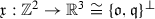
Example. Let $\mathfrak {Q}^3:=\{y\in \mathbb {R}^{4,1}\,|\,(y,y)=0,(y,q)=1\}$, where $\mathfrak {q}\in \mathbb {R}^{4,1}$ is isotropic, so that $\mathfrak {Q}^3\cong \mathbb {R}^3$. Namely, choose an “origin” $\mathfrak {o}\in \mathfrak {Q}^3$ (hence $\mathfrak {o}$ and $\mathfrak {q}$ span a Minkowski $\mathbb {R}^{1,1}\subset \mathbb {R}^{4,1}$) and observe that

(3.1)

is an isometry (in the differential geometric sense), cf [4, §9.3.2]. Suppose that $\mathfrak {s}:\mathbb {Z}^2\rightarrow \mathfrak {Q}^3$ is an affine projection of a Königs net in ${\mathbb {R}\!\textit{P}}^4$ so that its dual $\mathfrak {s}^*:\mathbb {Z}^2\rightarrow \mathfrak {Q}^3$ takes values in the same quadric $\mathfrak {Q}^3$ of (vanishing) constant sectional curvature,

using that $d\mathfrak {s}^*_{ij}={1\over \nu _i\nu _j}d\mathfrak {s}_{ij}$. Thus the stereographic projections of $s$ and $s^*$ are Königs dual circular nets⁵ at a constant distance, that is, they are parallel constant mean curvature nets in $\mathbb {R}^3$, with common Gauß map , in the sense of [9, Sect 5] or [4, Cor 4.53]. Thus requiring the dual of (an affine projection of) a Königs net in the quadric $\mathfrak {Q}^3$ to take values in the same quadric forces (the stereographic projection of) the discrete net to belong to the subclass of constant mean curvature nets. We shall see that this breaking of symmetry is systemic.

Note that this construction yields a transformation⁶ of discrete Königs nets in general quadrics: if the quadric is given as the projective null-cone of a non-degenerate inner product on $\mathbb {R}^5$ then a choice of a Minkowski plane, spanned by vectors $\mathfrak {o,q}$ as above, yields via “stereographic projection” a Königs net whose dual in $\{\mathfrak {o,q}\}^\perp$ lifts back to a Königs net in the quadric.

We aim to provide a similar characterization as the one for constant mean curvature nets in $\mathbb {R}^3$ above in the general case of an ambient space form geometry. Thus we consider the Möbius quadric (see [10, Chap 1] or [4, Sect 9.3])

$$\begin{aligned} S^3 = P(\mathcal{L}^4), \,\mathrm{where}\, \mathcal{L}^4 = \{y\in \mathbb {R}^{4,1}\,|\,(y,y)=0\} \end{aligned}$$

(3.2)

and $(.,.)$ denotes a Minkowski inner product on the space $\mathbb {R}^{4,1}\cong \mathbb {R}^5$ of homogeneous coordinates of ${\mathbb {R}\!\textit{P}}^4$. A Königs net $s:\mathbb {Z}^2\rightarrow S^3\subset {\mathbb {R}\!\textit{P}}^4$ then becomes circular: the intersection of $S^3\subset {\mathbb {R}\!\textit{P}}^4$ with the plane of each face yields the circumcircle of that face. That is, a discrete Königs net in $S^3$ is a discrete isothermic net, cf [4, Sect 4.3]:

3.1 Def. A discrete circular Königs net is called isothermic. A discrete net in $S^3\subset {\mathbb {R}\!\textit{P}}^4$ is isothermic if it is a discrete Königs net.

Alternatively, discrete isothermic nets can be characterized as circular nets so that the (real) cross ratios $[\mathfrak {s}_i,\mathfrak {s}_j,\mathfrak {s}_k,\mathfrak {s}_l]$ on elementary quadrilaterals $(ijkl)$ (as cross ratios of four points on a conic) factorize,

$$\begin{aligned}{}[s_i,s_j,s_k,s_l] = {a_{ij}\over a_{jk}}, \end{aligned}$$

(3.3)

where $(ij)\mapsto a_{ij}$ is an edge labelling, that is, an edge function ($a_{ij}=a_{ji}$) that is constant across opposite edges ($a_{ij}=a_{kl}$), see [4, Thm 4.25].

In consequence, the Christoffel formula (2.2) can be rewritten as (see [4, Thm 4.32])

$$\begin{aligned} d\mathfrak {s}^*= {a_{ij}\over |d\mathfrak {s}_{ij}|^2}\,d\mathfrak {s}_{ij}, \,\mathrm{where}\, a_{ij}={|d\mathfrak {s}_{ij}|^2\over \nu _i\nu _j}. \end{aligned}$$

(3.4)

In the presence of a non-degenerate inner product, an affine subgeometry is given by any choice of a non-zero $\mathfrak {q}\in \mathbb {R}^{4,1}$ via

$$\begin{aligned} \mathbb {R}^4 \cong \mathfrak {E}^4 : = \{\mathfrak {y}\in \mathbb {R}^{4,1}\,|\,(\mathfrak {y,q})=1\}, \end{aligned}$$

and the projection

$$\begin{aligned} \mathfrak {Q}^3 : = \mathcal{L}^4\cap \mathfrak {E}^4 \end{aligned}$$

(3.5)

of $S^3$ to $\mathfrak {E}^4$ is a quadric of constant sectional curvature $\kappa =-(\mathfrak {q,q})$, cf [10, Sect 1.4].

The characterization of Königs duality in Lemma 2.3 now suggests an intimate relation with the mean curvature of a discrete isothermic net defined via mixed areas (2.1):

3.2 Def. Let $\mathfrak {s}:\mathbb {Z}^2\rightarrow \mathfrak {Q}^3$ be a conjugate net; we say that a unit vector field $\mathfrak {n}:\mathbb {Z}^2\rightarrow S^{3,1}=\mathcal{L}^4_1$ (see below) is a Gauß map of $\mathfrak {s}$ if $\mathfrak {n}_i\in T_{\mathfrak {s}_i}\mathfrak {Q}^3$ at all vertices $i\in \mathbb {Z}^2$ and $\mathfrak {s}$ and $\mathfrak {n}$ are edge parallel, that is, if

$$\begin{aligned} (\mathfrak {n,s})\equiv 0 \,\, and \,\, d\mathfrak {n}_{ij} + k_{ij}d\mathfrak {s}_{ij} = 0 \end{aligned}$$

(3.6)

on all edges $(ij)$; the coefficients $k_{ij}$ yield the edge principal curvatures of the pair $(\mathfrak {s,n})$. Then the Gauß and mean curvature $K$ and $H$, respectively, of the pair $(\mathfrak {s,n})$ are defined by the equations

$$\begin{aligned} A(\mathfrak {n,n}) = KA(\mathfrak {s,s}) \,\,\textit{and}\,\, A(\mathfrak {n,s}) = -HA(\mathfrak {s,s}). \end{aligned}$$

A discrete conjugate net in a quadric $\mathfrak {Q}^3$ of constant curvature is circular, as discussed above, hence always admits a Gauss map in the sense of this definition. Note that both, mean and Gauß curvature, are defined on faces of a conjugate or isothermic net in this way.

In the affine subgeometry of $\mathfrak {E}^4$ it also makes sense to consider “concentric quadrics”, see Fig 4.

Fig. 4

Concentric quadrics

3.3 Def. Given an affine projection of $S^3$ to a quadric $\mathfrak {Q}^3$ of constant curvature in an affine subgeometry of ${\mathbb {R}\!\textit{P}}^4$, we define its concentric quadrics as

$$\begin{aligned} \mathfrak {Q}^3_{r,t} := \mathcal{L}^4_t\cap \mathfrak {E}^4_r, \, \textit{where}\,{\left\{ \begin{array}{ll} \mathfrak {E}^4_r := \{\mathfrak {y}\in \mathbb {R}^{4,1}\,|\,(\mathfrak {y,q})=r\}, \\ \mathcal{L}^4_t := \{y\in \mathbb {R}^{4,1}\,|\,(y,y)=t\}. \end{array}\right. } \end{aligned}$$

(3.7)

Note that we consider the full $2$-parameter family of quadrics $\mathfrak {Q}^3_{r,t}$ as “concentric quadrics”, though we shall see below that generically the family is essentially $1$-dimensional when using suitable identifications.

These concentric quadrics lie in parallel affine subgeometries $\mathfrak {E}^4_r$, allowing their identification via projection along $\mathfrak {q}$. The terminology “concentric” is motivated by the case $(\mathfrak {q,q})\ne 0$, where the hyperplanes $\mathfrak {E}^4_r$ inherit a non-degenerate inner product and the points $\mathfrak {c}_r:={r\mathfrak {q}\over (\mathfrak {q,q})}\in \mathfrak {E}^4_r$ can be identified with a common centre of the quadrics⁷:

$$\begin{aligned} \mathfrak {Q}^3_{r,t} = \{ \mathfrak {y\in E}^4_r \,|\, (\mathfrak {y-c}_r,\mathfrak {y-c}_r) = t-{r^2\over (\mathfrak {q,q})} = {r^2+t\kappa \over \kappa } \}. \end{aligned}$$

(3.8)

Thus the quadrics $\mathfrak {Q}^3_{r,t}$ and $\mathfrak {Q}^3_{r',t'}$ with $r^2+t\kappa =r'^2+t'\kappa$ can be identified via parallel projection along $\mathfrak {q}$.

In the degenerate case $(\mathfrak {q,q})=0$ the quadrics $\mathfrak {Q}^3_{r,t}$ can simultaneously and isometrically be parametrized over the Euclidean space $\mathbb {R}^3\cong \{\mathfrak {o,q}\}^\perp$ by

(3.9)

as long as $r\ne 0$, and after choosing⁸ an origin $\mathfrak {o\in Q}^3=\mathfrak {Q}^3_{1,0}$ for the stereographic projection. This shows that the “concentric quadrics” become a translation family of paraboloids. When $r=0$, on the other hand, $\mathfrak {Q}^3_{0,t}$ becomes a circular cylinder of radius $t>0$ and with isotropic generators.

Now suppose that there is an affine projection $\mathfrak {s}:\mathbb {Z}^2\rightarrow \mathfrak {Q}^3$ of our Königs net $s:\mathbb {Z}^2\rightarrow S^3$, so that its Königs dual⁹

$$\begin{aligned} \mathfrak {s}^*:\mathbb {Z}^2\rightarrow \mathfrak {Q}^3_{r,t} \end{aligned}$$

takes values in one of the concentric quadrics $\mathfrak {Q}^3_{r,t}$.

As both $(\mathfrak {s,s}),(\mathfrak {s^*,s^*})\equiv \mathrm{const}$, we learn that $(\mathfrak {s}_{ij},d\mathfrak {s}_{ij}) = (\mathfrak {s}^*_{ij},d\mathfrak {s}^*_{ij}) = 0$ on any edge $(ij)$ of $\mathbb {Z}^2$; hence,

$$\begin{aligned} d(\mathfrak {s,s}^*)_{ij} = (d\mathfrak {s}_{ij},\mathfrak {s}^*_{ij}) + (\mathfrak {s}_{ij},d\mathfrak {s}^*_{ij}) = 0 \end{aligned}$$

since $\mathfrak {s}$ and $\mathfrak {s}^*$ have parallel edges, which shows that:

3.4 Lemma. For Königs dual nets $\mathfrak {s}$ and $\mathfrak {s}^*$ in concentric quadrics we have $(\mathfrak {s,s}^*)\equiv \mathrm{const}$. When $r=1$ then $\mathfrak {s}$ and $\mathfrak {s}^*$ lie in the same affine space $\mathfrak {E}^4$ at constant distance $|\mathfrak {s^*-s}|^2=t-2(\mathfrak {s,s^*})$.

In the positive definite case, where $\mathfrak {s}$ and $\mathfrak {s}^*$ take values in two concentric spheres, this result can alternatively be obtained by a pretty and more geometric argument, cf Fig 5: restricting focus to the plane containing two corresponding edges $d\mathfrak {s}_{ij}$ and $d\mathfrak {s}^*_{ij}$, we obtain a figure of two parallel segments in concentric circles — which therefore form an equilateral trapezoid.

Fig. 5

Constant distance in the sphere case $|\mathfrak {q}|^2<0$

3.5 Thm. If a Königs net $s:\mathbb {Z}^2\rightarrow S^3\subset {\mathbb {R}\!\textit{P}}^4$ admits an affine projection $\mathfrak {s}$ so that its Königs dual $\mathfrak {s}^*$ takes values in a concentric ¹⁰ quadric (3.7) then $\mathfrak {s}$ has constant mean curvature $H$.

In order to prove Thm 3.5 we wish to show that the mixed area mean curvature with respect to a suitable tangent plane congruence $\mathfrak {t}$ for $\mathfrak {s}$ is constant. Thus set

$$\begin{aligned} \mathfrak {t} : = \mathfrak {s}^*+ ({\mathfrak {(}s,s^*)(q,q)}-r)\,\mathfrak {s} - {\mathfrak {(}s,s^*)\,q} \end{aligned}$$

(3.10)

and observe that $\mathfrak {t\in \{s,q\}^\perp }=T_{\mathfrak {s}}\mathfrak {Q}^3$; in particular, $(\mathfrak {t,t})>0$ unless $\mathfrak {t}=0$ since $\mathfrak {Q}^3$ is a Riemannian quadric of constant curvature. As

$$\begin{aligned} (\mathfrak {t,t}) = t - 2r(\mathfrak {s,s^*}) + (\mathfrak {q,q})(\mathfrak {s,s^*})^2 \equiv \mathrm{const}\end{aligned}$$

(3.11)

we learn that $\mathfrak {t}_i\ne 0$ at all points $i\in \mathbb {Z}^2$ except when $\mathfrak {s}$ is “self-dual”, that is, $\mathfrak {s}^*$ is obtained from $\mathfrak {s}$ by a homothety and a translation. Excluding this self-dual case, $\mathfrak {t}$ defines a suitable tangent plane congruence of $\mathfrak {s}$ in the sense that the pair $(\mathfrak {s,t})$ becomes a principal contact element net [4, Def 3.24] or discrete “Legendre map” [7, Def 3.1] as $\mathfrak {t}$ and $\mathfrak {s}$ have parallel edges: with the (edge) principal curvatures $k_{ij}$ defined by $0 = d\mathfrak {t}_{ij} + k_{ij}\,d\mathfrak {s}_{ij},$ cf (3.6), we obtain

$$\begin{aligned} \kappa _{ij} : = \mathfrak {t}_i + k_{ij}\mathfrak {s}_i = \mathfrak {t}_j + k_{ij}\mathfrak {s}_j \end{aligned}$$

as the common (curvature) spheres associated to an edge. Note that, in the non-degenerate case $(\mathfrak {q,q})\ne 0$ and denoting $\mathfrak {c}_r={r\mathfrak {q}\over {\mathfrak {(}q,q)}}$ as before,

$$\begin{aligned} \mathfrak {t} = (\mathfrak {s^*-c}_r) + \{{\mathfrak {(}s,s^*)(q,q)}-r\}(\mathfrak {s-c}_1). \end{aligned}$$

(3.12)

Thus the mixed area mean curvature of $\mathfrak {s}:\mathbb {Z}^2\rightarrow \mathfrak {Q}^3$ with respect to $\mathfrak {n}:={1\over \sqrt{\mathfrak {(}t,t)}}\,\mathfrak {t}$ as a Gauß map is now determined from

$$\begin{aligned} 0 = H\,A(\mathfrak {s,s}) + A(\mathfrak {s,n}) = \{ H + {{\mathfrak {(}s,s^*)(q,q)}-r\over \sqrt{\mathfrak {(}t,t)}} \}\, A(\mathfrak {s,s}) \end{aligned}$$

since $A(\mathfrak {s,s^*})=A(\mathfrak {s,q})=0$. Hence $\mathfrak {s}$ has constant mean curvature with respect to $\mathfrak {n}$, proving Thm 3.5.

4 Königs duality via constant mean curvature

To see that, conversely, every constant mean curvature net $\mathfrak {s}$ in a quadric $\mathfrak {Q}^3$ of constant sectional curvature, given in (3.5), arises via Königs duality in concentric quadrics we shall construct a suitable dual for a given net $\mathfrak {s}:\mathbb {Z}^2\rightarrow \mathfrak {Q}^3$ with Gauß map $\mathfrak {n}$ that has constant mean curvature $H$ in the mixed area sense: $0 = A(\mathfrak {n,s}) + H\,A(\mathfrak {s,s}).$

Thus we use the “mean curvature sphere congruence”¹¹ of the pair $(\mathfrak {s,n})$ to obtain a prototype Königs dual for $\mathfrak {s}$:

4.1 Lemma & Def. Suppose the $(\mathfrak {s,n})$ has constant mean curvature $H$ in a quadric $\mathfrak {Q}^3$ of constant curvature. Then $\mathfrak {s}:\mathbb {Z}^2\rightarrow \mathfrak {E}^4$ has a Königs dual $\mathfrak {z}$ in the parallel affine subgeometry $\mathfrak {E}^4_H$ given by

$$\begin{aligned} \mathfrak {z} : = \mathfrak {n} + H\mathfrak {s}:\mathbb {Z}^2\rightarrow \mathfrak {E}^4_H\subset \mathbb {R}^{4,1} \end{aligned}$$

(4.1)

The sphere congruence $z=\mathbb {R}\mathfrak {z}:\mathbb {Z}^2\rightarrow {\mathbb {R}\!\textit{P}}^4$ will be called the mean curvature sphere congruence of $(\mathfrak {s,n})$.

Clearly $A(\mathfrak {z,s})=0$ and $(\mathfrak {z,q})=H$, so that $\mathfrak {s}$ and $\mathfrak {z}$ are Königs dual nets in the parallel affine subgeometries of $\mathfrak {E}^4$ and $\mathfrak {E}^4_H$, respectively, by Lemma 2.3. This proves Lemma 4.1.

The converse of Thm 3.5 is now a straightforward consequence:

4.2 Thm. Let $\mathfrak {s}:\mathbb {Z}^2\rightarrow \mathfrak {Q}^3$ be a discrete isothermic net in a quadric of constant curvature $\kappa$ with constant mean curvature $H$ with respect to a Gauß map $\mathfrak {n}$. Then its mean curvature sphere congruence $z$ projects to a Königs dual net $\mathfrak {s}^*=\mathfrak {z}$ in a concentric quadric $\mathfrak {Q}^3_{r,t}$.

Namely, $(\mathfrak {z,z})=1$ so that $\mathfrak {s}$ and $\mathfrak {z}$ take values in the concentric quadrics $\mathfrak {Q}^3$ and $\mathfrak {Q}^3_{H,1}$, proving the theorem.

Note that the Königs dual projection of the mean curvature sphere congruence is not unique: as Königs duality is invariant under homotheties and translations, the nets

$$\begin{aligned} \mathfrak {s}^*: = \lambda \mathfrak {z}+\mu \mathfrak {q}:\mathbb {Z}^2\rightarrow \mathfrak {Q}^3_{r,t}, \,\mathrm{where}\, {\left\{ \begin{array}{ll} r=\lambda H-\mu \kappa , \, \\ t=\lambda ^2+2\lambda \mu H-\mu ^2\kappa , \end{array}\right. } \end{aligned}$$

(4.2)

yield Königs duals into a family of concentric quadrics. Identifying parallel affine subgeometries via projection along $\mathfrak {q}$ this is a $1$-parameter family: in the non-flat cases $\kappa \ne 0$ we learn from (3.8) that the translation part given by $\mu$ plays no geometric role as

$$\begin{aligned} \mathfrak {Q}^3_{r,t} = \{ \mathfrak {y\in E}^4_r\,|\, (\mathfrak {y-c}_r,\mathfrak {y-c}_r) = \lambda ^2{H^2+\kappa \over \kappa } \}, \end{aligned}$$

(4.3)

whereas this becomes clear from the parametrizations given in (3.9) in the flat case:

(4.4)

In the case $H=\kappa =0$, where $\mathfrak {s}$ is a discrete Euclidean minimal surface, $\mathfrak {s}^*$ takes values in an isotropic cylinder of radius $\lambda$ and axis $\mathfrak {q}$ and projects to the Euclidean Gauß map of the minimal net in $\mathbb {R}^3$.

Note that we obtain a Königs dual net $\mathfrak {s}^*$ in the original quadric $\mathfrak {Q}^3=\mathfrak {Q}^3_{1,0}$ from (4.2) if and only if the Lawson invariant $H^2+\kappa >0$, with

$$\begin{aligned} \lambda = \pm {1\over \sqrt{H^2+\kappa }} \,\mathrm{and}\, \mu = \mp {1\over \sqrt{H^2+\kappa }(H\pm \sqrt{H^2+\kappa })}. \end{aligned}$$

As we have now identified the Königs nets in a quadric of constant curvature that have a Königs dual in a concentric quadric as the mixed area constant mean curvature nets, it follows from [7] that these are precisely the constant mean curvature nets in the sense of [6].

In fact, our “mean curvature sphere congruence” $\mathfrak {z}$ is that of [6, Def 5.1], cf [7, Expl 4.2], and in case of a positive Lawson invariant $H^2+\kappa >0$ the duals $\mathfrak {s}^*:\mathbb {Z}^2\rightarrow \mathfrak {Q}^3=\mathfrak {Q}^3_{1,0}$ obtained from (4.2) are the “complementary nets” of [6, Sect 4.3]: special Darboux transforms of an isothermic net¹² whose existence is characteristic for discrete isothermic nets of constant mean curvature, cf [9, Sect 5] and our starting example. We omit a detailed analysis to substantiate these claims here, as it would require a discussion of the highly non-trivial techniques introduced in [6], where the reader is referred for further details.

However, as a consequence, examples and constructions of classes of discrete constant mean curvature nets from the latter theory apply in our approach: for example, the discrete minimal catenoid of [11] or, more generally, the construction of discrete constant mean curvature surfaces of revolution in space forms provided there show that our theory is not empty. A less involved example of a dual pair of discrete constant mean curvature nets in the $3$-sphere is discussed below.

5 Discrete cmc surfaces in space forms

Thus we have obtained a characterization of discrete constant mean curvature nets (in the sense of mixed areas) in space forms, that is, simply connected complete spaces of constant sectional curvature (as modeled by our quadrics $\mathfrak {Q}^3=\mathfrak {Q}^3_{1,0}$), via Königs duality:

5.1 Cor. A Königs net $s:\mathbb {Z}^2\rightarrow S^3$ projects to a constant mean curvature net $\mathfrak {s}$ in a quadric $\mathfrak {Q}^3$ of constant curvature if and only if a Königs dual of the projection takes values in a concentric quadric $\mathfrak {Q}^3_{r,t}$; the Gauß map $\mathfrak {n}$ of $\mathfrak {s}$ is obtained by projecting the vector field joining $\mathfrak {s}$ and its dual $\mathfrak {s}^*$ onto the tangent bundle of $\mathfrak {Q}^3$.

In the case $\kappa \ne 0$ of a non-flat ambient geometry, the latter assertion follows directly from (3.12) as

$$\begin{aligned} \mathfrak {t} = (\mathfrak {s^*-c}_r) - (r+\kappa (\mathfrak {s,s^*}))(\mathfrak {s-c}_1) \end{aligned}$$

while, in the case $\kappa =0$ of a flat ambient geometry, the parametrizations (3.9) reduce (3.10) to

Constant mean curvatures surfaces in space forms come in different types, depending on the sign of $H^2+\kappa$ or, equivalently, depending on whether the Gauß equation reduces to the $\sinh$-Gordon equation, the Liouville equation or the $\cosh$-Gordon equation, respectively. We shall see that these types are reflected in the geometry of the Königs dual $\mathfrak {s}^*$ as well. To see this, we first note that $H^2+\kappa ={r^2+t\kappa \over (\mathfrak {t,t})}$ using (3.11); in particular, the sign of $H^2+\kappa$ is the same as that of $r^2+t\kappa$, showing that the ambient geometry of the Königs dual $\mathfrak {s}^*$ is related to the sign of $H^2+\kappa$, see (3.8).

With this in mind we now provide a detailed analysis of the occurring cases, cf Fig 6.

• (i) $H^2+\kappa >0$: these surfaces arise in all space forms.

  • (a) Any constant mean curvature net in a spherical ambient geometry, $\kappa >0$, belongs to this class as $H^2+\kappa >0$. The affine geometries of $\mathfrak {E}^4_r$ are all Euclidean geometries and (4.3) shows that the quadrics $\mathfrak {Q}^3_{r,t}$ are concentric $3$-spheres. Rescaling (in $\mathfrak {E}^4_r$) and shifting $\mathfrak {s}^*$ into $\mathfrak {E}^4$,

    $$\begin{aligned} \mathfrak {s}^*\rightarrow \pm {1\over \sqrt{r^2+t\kappa }}(\mathfrak {s^*-c}_r) + \mathfrak {c}_1 = \pm {1\over \sqrt{H^2+\kappa }}(\mathfrak {z}+{H\over \kappa }\mathfrak {q}) - {1\over \kappa }\mathfrak {q}, \end{aligned}$$

    (5.1)

    yields either of two antipodal Königs duals in $\mathfrak {Q}^3$, that have constant (chordal) distances $\sqrt{{2\over \kappa }(1\mp {H\over \sqrt{H^2+\kappa }})}$ from $\mathfrak {s}$: these form a pair of antipodal Darboux transforms of $\mathfrak {s}$, whose existence also characterizes discrete constant mean curvature nets in a spherical geometry, see [6, Sect 5.2].

    Fig. 6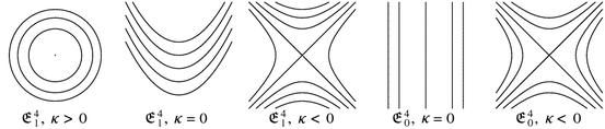

    

    Concentric quadrics

  • (b) In Euclidean geometry, $\kappa =0$, any non-minimal constant mean curvature net belongs to the class under consideration. The affine geometries of $\mathfrak {E}^4_r$ inherit a degenerate metric from $\mathbb {R}^{4,1}$ and from (4.4) we learn that the quadrics $\mathfrak {Q}^3_{r,t}$ are a translation family of paraboloids. Suitably rescaling and shifting $\mathfrak {s}^*$ again,

    $$\begin{aligned} \mathfrak {s}^*\rightarrow {1\over r}(\mathfrak {s}^*- {t\over 2r}\mathfrak {q}) = {1\over H}(\mathfrak {z}-{1\over 2H}\mathfrak {q}), \end{aligned}$$

    (5.2)

    places the Königs dual in $\mathfrak {Q}^3$ at a distance¹³ ${1\over H}$ from $\mathfrak {s}$: using the parametrization

    

    of (3.9), where $\mathfrak {g}$ denotes a Euclidean Gauß map of in $\mathbb {R}^3=\{\mathfrak {o,q}\}^\perp$, we obtain

    

    Thus we recover the characterization of constant mean curvature nets from [2, Sect 4], or from [9, Sect 5] as this Königs dual at constant distance is also a Darboux transform of $s$.

  • (c) In the hyperbolic case, $\kappa <0$, the absolute value of the mean curvature $H$ must be greater than that of a horosphere for a constant mean curvature net to belong to the considered class. Algebraically, the analysis of these nets is identical to the spherical case, but their geometric interpretation becomes different: now the affine geometries of $\mathfrak {E}^4_{r,t}$ inherit a Minkowski inner product from $\mathbb {R}^{4,1}$ and (4.3) shows that the quadrics $\mathfrak {Q}^3_{r,t}$ are two-sheeted hyperboloids. The rescaling and shift from (5.1) places the Königs dual $\mathfrak {s}^*$ in either of the two sheets of $\mathfrak {Q}^3$, so that they are “antipodal”, that is, they can be identified via reflection in the infinity boundary of $\mathfrak {Q}^3$. Consequently, the squares of their constant chordal distances ${2\over \kappa }(1\mp {H\over \sqrt{H^2+\kappa }})$ to $\mathfrak {s}$ have different signs. Again, both are Darboux transforms of $s$, placing us in the situation analyzed in [6, Sect 5.2].

• (ii) $H^2+\kappa =0$: for this to hold we must have $\kappa \le 0$, that is, these surfaces only occur in Euclidean or hyperbolic geometries.

  • (b) In the Euclidean case, $\kappa =0$, we consider minimal nets in $\mathbb {R}^3$: the affine geometry of $\mathfrak {E}^4_0$ inherits again a degenerate inner product and the Königs dual $\mathfrak {s}^*$ of $\mathfrak {s}$ takes values in an isotropic cylinder $\mathfrak {Q}^3_{0,t}\cong S^2(\sqrt{t})\times \mathbb {R}\mathfrak {q}$, $t>0$. Thus, using the parametrization from (3.9) for $\mathfrak {s}:\mathbb {Z}^2\rightarrow \mathfrak {Q}^3=\mathfrak {Q}^3_{1,0}$,

    

    where $\mathfrak {g}:\mathbb {Z}^2\rightarrow S^2$ is a Euclidean Gauß map of that renders into a minimal net in $\mathbb {R}^3$ in the sense of [1, Thm 8]. Note that, while $|\mathfrak {z-s}|^2=-2(\mathfrak {z,s})\equiv 0$, shifting $\mathfrak {s\rightarrow s-o}$ into the parallel affine subgeometry $\mathfrak {E}^4_0$ of $\mathfrak {z}$, their “distance” $|\mathfrak {z-s+o}|^2=(2\mathfrak {g-x,x})$ does not remain constant. Also, in contrast to the case $H^2+\kappa >0$, the Königs dual $\mathfrak {s}^*$ cannot be placed in $\mathfrak {Q}^3$. Consequently, it does not give rise to a Darboux transform of $s$ in the sense of the isothermic transformation theory of discrete isothermic nets in $S^3$.

  • (c) When $\kappa <0$ we are considering “horospherical nets” in a hyperbolic geometry: $\mathfrak {s}$ then has the same constant mean curvature as a horosphere of the ambient hyperbolic geometry. Now the affine subgeometry of $\mathfrak {E}^4_r$ inherits a Minkowski inner product from $\mathbb {R}^{4,1}$ and from (4.3) we find that $\mathfrak {Q}^3_{r,t}$ becomes the light cone of this Minkowski $4$-space. Shifting both, $\mathfrak {s}$ and $\mathfrak {s}^*$ into the same affine plane, say $\mathfrak {E}^4_0$:

    $$\begin{aligned} \mathfrak {s\rightarrow s-c}_1 \,\mathrm{and}\, \mathfrak {s^*\rightarrow s^*-c}_r, \end{aligned}$$

    their distance $|(\mathfrak {s^*-c}_r)-(\mathfrak {s-c}_1)|^2 = {1-2r\over \kappa }-2(\mathfrak {s,s^*})$ in $\mathfrak {E}^4_0$ is constant by Lemma 3.4. On the other hand, $\mathfrak {s},\mathfrak {s-c}_r:\mathbb {Z}^2\rightarrow \mathcal{L}^4$ yield maps into $S^3\subset {\mathbb {R}\!\textit{P}}^4$, allowing to interpret them as Darboux transforms of each other — which recovers the characterization of horospherical nets of [10, §5.7.37] via the existence of a “hyperbolic Gauß map” as a totally umbilic Darboux transform.

• (iii) $H^2+\kappa <0$: these surfaces only occur in hyperbolic geometry and include the interesting case of hyperbolic minimal surfaces, such as the minimal catenoid of [11].

  • (c) As $\kappa <0$, the affine ambient geometry of the Königs dual $\mathfrak {s}^*$ of $\mathfrak {s}$ inherits again a Minkowski inner product. The target quadric $\mathfrak {Q}^3_{r,t}$ of $\mathfrak {s}^*$ now becomes a one-sheeted hyperboloid, see (4.3). Arbitrarily rescaling $\mathfrak {s}^*$ (in $\mathfrak {E}^4_r$) and shifting it into the affine ambient space $\mathfrak {E}^4$ of $\mathfrak {s}$,

    $$\begin{aligned} \mathfrak {s}^*\rightarrow \lambda (\mathfrak {s-c}_r) + \mathfrak {c}_1, \end{aligned}$$

    we obtain a Königs dual pair in $\mathfrak {E}^4$ at a constant distance. However, as in the case of minimal nets in Euclidean geometry, $\mathfrak {s}^*$ cannot be placed in (an affine projection of) the Möbius quadric $S^3\subset {\mathbb {R}\!\textit{P}}^4$, so that an interpretation of the dual as a Darboux transformation of $s:\mathbb {Z}^2\rightarrow S^3$ is not available.

Thus, while in Euclidean and hyperbolic ambient geometries constant mean curvature nets occur in different flavours, a beautiful and simple result emerges in spherical ambient geometry:

5.2 Cor. A Königs net $\mathfrak {s}:\mathbb {Z}^2\rightarrow S^3$ possesses a unit normal field $\mathfrak {n}:\mathbb {Z}^2\rightarrow S^3$ so that $(\mathfrak {s,n})$ has constant mean curvature if and only if $\mathfrak {s}$ admits a (pair of antipodal) Königs dual(s) in $S^3\subset \mathbb {R}^4$.

Example. A simple example, beautifully illustrating this corollary, is given by the Clifford tori in $S^3$. Fixing a timelike vector $\mathfrak {q}\in \mathbb {R}^{4,1}$, $(\mathfrak {q,q})=-1$, the affine hyperplane $\mathfrak {E}^4=\mathfrak {E}^4_1\cong \mathbb {R}^4$ and $\mathfrak {Q}^3=\mathfrak {Q}^3_{1,0}\cong S^3$ becomes the unit sphere in this Euclidean $4$-space. Now let $\varphi ,\psi :\mathbb {Z}\rightarrow \mathbb {R}$ be two (strictly increasing) functions that project to periodic $\mathbb {R}/(2\pi \mathbb {Z})$-valued functions, that is, $\varphi (m+m_0)=\varphi (m)+2\pi$ and $\psi (n+n_0)=\psi (n)+2\pi$ for some $m_0,n_0\in \mathbb {N}$, let $\alpha \in (0,{\pi \over 2})$, and define¹⁴

$$\begin{aligned} \mathfrak {s} : = \left( \begin{array}{c}e^{i\varphi }\cos \alpha \\ e^{i\psi }\sin \alpha \end{array}\right) \,\mathrm{and}\, \mathfrak {n} : = \left( \begin{array}{c}-e^{i\varphi }\sin \alpha \\ e^{i\psi }\cos \alpha \end{array}\right) , \end{aligned}$$

where we identify $\mathbb {R}^4\cong \mathbb {C}^2$. Clearly, $\mathfrak {s,n}:\mathbb {Z}^2\rightarrow S^3$ and $\mathfrak {n}\perp \mathfrak {s}$. Moreover, $\mathfrak {s}$ and $\mathfrak {n}$ are edge parallel,

$$\begin{aligned} 0 = (d\mathfrak {n} + \tan \alpha \,d\mathfrak {s})_{(m,n)(m+1,n)} = (d\mathfrak {n} - \cot \alpha \,d\mathfrak {s})_{(m,n)(m,n+1)}, \end{aligned}$$

when $\varphi =\varphi (m)$ and $\psi =\psi (n)$, so that $\mathfrak {s}$ has (edge) principal curvatures $\tan \alpha$ and $-\cot \alpha$ with respect to $\mathfrak {n}$ as a Gauß map. To determine the (face) mean curvature note that $\mathfrak {s}$ and

$$\begin{aligned} \mathfrak {z} : = \mathfrak {n}-\cot 2\alpha \,\mathfrak {s} = {1\over \sin 2\alpha }\left( \begin{array}{c} -e^{i\varphi }\cos \alpha \\ e^{i\psi }\sin \alpha \end{array}\right) \end{aligned}$$

have parallel opposite diagonals,

$$\begin{aligned} \delta \mathfrak {z}_{(m,n)(m+1,n+1)} \parallel \delta \mathfrak {s}_{(m+1,n)(m,n+1)} \,\mathrm{and}\, \delta \mathfrak {z}_{(m+1,n)(m,n+1)} \parallel \delta \mathfrak {s}_{(m,n)(m+1,n+1)}, \end{aligned}$$

showing that

$$\begin{aligned} 0 = A(\mathfrak {z,s}) = A(\mathfrak {n,s}) - \cot 2\alpha \,A(\mathfrak {s,s}), \,\mathrm{hence}\, H \equiv -\cot 2\alpha . \end{aligned}$$

Note that, in this case, we obtain the mean curvature as the arithmetic mean of the principal curvatures of the edges of a face — in general, this relation is far more intricate, cf [5, Prop 11]. Further, two (antipodal) dual nets of $\mathfrak {s}$ in $S^3\subset \mathbb {R}^4\cong \mathfrak {E}^4$ are obtained as

$$\begin{aligned} \mathfrak {s}^*= \pm \sin 2\alpha \,\mathfrak {z} = \pm (\sin 2\alpha \,\mathfrak {n} - \cos 2\alpha \,\mathfrak {s}). \end{aligned}$$

Note that in the case $\alpha ={\pi \over 4}$ of a minimal (square) Clifford torus $\mathfrak {s}^*=\pm \mathfrak {n}=\pm \mathfrak {z}$. If $\varphi$ or $\psi$ projects to a periodic $\mathbb {R}/(\pi \mathbb {Z})$-valued function, with periods $m_1={m_0\over 2}$ or $n_1={n_0\over 2}$, then the minimal Clifford torus becomes “self-dual” in the sense that

$$\begin{aligned} \mathfrak {s}^*_{m,n} = \pm \mathfrak {s}_{m+m_1,n} \,\mathrm{or}\, \mathfrak {s}^*_{m,n} = \mp \mathfrak {s}_{m,n+n_1}. \end{aligned}$$

References

Bobenko, A., Pinkall, U.: Discrete isothermic surfaces. J. Reine Angew Math. 475, 187–208 (1996)
Bobenko, A., Pinkall, U.: Discretization of surfaces and integrable systems. Oxf. Lect. Ser. Math. Appl. 16, 3–58 (1999)
Bobenko, A., Hoffmann, T., Springborn, B.: Minimal surfaces from circle patterns: geometry from combinatorics. Ann. Math. 164, 231–264 (2006)
Bobenko, A., Suris, Y.: Discrete Differential Geometry. Integrable Structure, Graduate Studies in Mathematics. American Mathematical Society, Providence, RI (2008)
Bobenko, A., Pottmann, H., Wallner, J.: A curvature theory for discrete surfaces based on mesh parallelity. Math. Ann. 348, 1–24 (2010)
Burstall, F., Hertrich-Jeromin, U., Rossman, W., Santos, S.: Discrete surfaces of constant mean curvature. RIMS Kokyuroku 1880, 133–179 (2014)
Burstall, F., Hertrich-Jeromin, U., Rossman, W.: Discrete linear Weingarten surfaces, arXiv:1406.1293 (2014).
Große-Brauckmann, K., Polthier, K.: Numerical examples of compact constant mean curvature surfaces. In: Chow, B. (ed.) Elliptic and Parabolic Methods in Geometry, pp. 23–46. CRC Press, Boca Raton (1996)
Hertrich-Jeromin, U., Hoffmann, T., Pinkall, U.: A discrete version of the Darboux transform for isothermic surfaces. Oxf. Lect. Ser. Math. Appl. 16, 59–81 (1999)
Hertrich-Jeromin, U.: Mathematical Society Lecture Note Series. Introduction to Möbius differential geometry. Cambridge University Press, Cambridge (2003)
Hertrich-Jeromin, U., Rossman, W.: Discrete minimal catenoid in hyperbolic 3-space. Electr Geom Model 2010.11.001 (2010).
Hoffmann, T., Rossman, W., Sasaki, T., Yoshida, M.: Discrete flat surfaces and linear Weingarten surfaces in hyperbolic \(3\)-space. Trans. AMS 364, 5605–5644 (2012)
Pinkall, U., Polthier, K.: Computing discrete minimal surfaces and their conjugates. Exp. Math. 2, 15–36 (1993)
Schief, W.: On the unification of classical and novel integrable surfaces II. Difference geometry. Proc. R. Soc. Lond. A 459, 2449–2462 (2003)
Schief, W.: On a maximum principle for minimal surfaces and their integrable discrete counterparts. J. Geom. Phys. 56, 1484–1495 (2006)
Acknowledgments
We would like to thank F. Burstall and W. Rossman for fruitful and enjoyable discussions. Thanks also go to the referees whose comments greatly helped to improve the text.
Author information
Authors and Affiliations
Corresponding author
Additional information
Partially supported by the DFG Collaborative Research Center TRR 109, “Discretization in Geometry and Dynamics”.
Rights and permissions
About this article
Cite this article
Bobenko, A.I., Hertrich-Jeromin, U. & Lukyanenko, I. Discrete constant mean curvature nets in space forms: Steiner’s formula and Christoffel duality. Discrete Comput Geom 52, 612–629 (2014). https://doi.org/10.1007/s00454-014-9622-5
Received:
Revised:
Accepted:
Published:
Issue Date:
DOI: https://doi.org/10.1007/s00454-014-9622-5
Keywords
- Königs dual
- Christoffel transformation
- Discrete conjugate net
- Space form
- Constant mean curvature