
Abstract
Tree-ring chronologies are the main source for annually resolved and absolutely dated temperature reconstructions of the last millennia and thus for studying the intriguing problem of climate impacts. Here we focus on central Europe and compare the tree-ring based temperature reconstruction with reconstructions from harvest dates, long meteorological measurements, and historical model data. We find that all data are long-term persistent, but in the tree-ring based reconstruction the strength of the persistence quantified by the Hurst exponent is remarkably larger (\(h\cong 1.02\)) than in the other data (\(h=\) 0.52–0.69), indicating an unrealistic exaggeration of the historical temperature variations.We show how to correct the tree-ring based reconstruction by a mathematical transformation that adjusts the persistence and leads to reduced amplitudes of the warm and cold periods. The new transformed record agrees well with both the observational data and the harvest dates-based reconstructions and allows more realistic studies of climate impacts. It confirms that the present warming is unprecedented.
1 Introduction
One of the important questions in global change research is which impact the increase of the recent warming will have on societies and human beings (Stocker et al. 2013). One possibility to study this question is to look at historical developments in relation to annually resolved and absolutely dated temperature reconstructions.
Presently, the main source for these kinds of data are tree-ring chronologies that in some cases cover more than two millennia (Esper et al. 2016). However, the reliability of their high-frequency variability (Matalas 1962; Cook et al. 1999) as well as, their low-frequency variability (von Storch et al. 2004; Moberg 2012; Franke et al. 2013; Bunde et al. 2013) is debated and it is not yet clear to which extent tree-ring chronologies reflect historical reality.
The purpose of this article is to assess and improve tree-ring based reconstructions of temperatures. We focus on central Europe, where the temperatures of the past can be obtained not only from tree-rings (Büntgen et al. 2011), but also from long meteorological measurements (1753-present) (Berkley Earth; Czech Hydrometeorological Institute) as well as from grape and rye harvests date records (Chuine et al. 2004; Labbé and Gaveau 2011; Meier et al. 2007; Wetter and Pfister 2011) that date back up to 1370 and from historical model data (850-1849) (Jungclaus et al. 2010; Earth System Grid Federation).
Figure 1a shows the tree-ring based reconstruction (TRBR) of central European summer temperatures (Büntgen et al. 2011), together with its 30 year moving average that reveals the long-term temperature variations in the record. Particularly large temperature increases occurred between 1340 and 1410 and between 1820 and 1870 that even are comparable in amplitude with the recent warming trend since 1970, indicating that the recent (anthropogenic) warming may not be unprecedented.
To assess if the amplitudes of the warm and cold periods in the reconstructed temperature record reflect reality, we first performed a persistence analysis of the TRBR record and compared it with the results from the other three sources. We find that all records are long-term persistent. The strength of the long-term persistence is quantified by the Hurst exponent h. This exponent was originally introduced by Harold E. Hurst to quantify the persistence in streamflow data of the Nile (Hurst 1951) and has since then been applied to a large number of records in hydrology, climate, financial markets and biology (see, e.g., Bunde et al. 2012). Here we show, that the strength of the long term persistence is remarkably larger in the TRBR record than in the other time series. We demonstrate that it is this overestimation of the long-term persistence that leads to the enormous climate variations in the tree-ring based reconstruction and discuss its potential origin. Finally, we show how the TRBR record can be corrected by a mathematical transformation that reduces the Hurst exponent and leads to reduced amplitudes of the warm and cold periods while leaving their positions unchanged. The transformed record agrees well with both the observational data and the harvest dates based temperature reconstructions and also confirms unprecedented recent warming in central Europe.
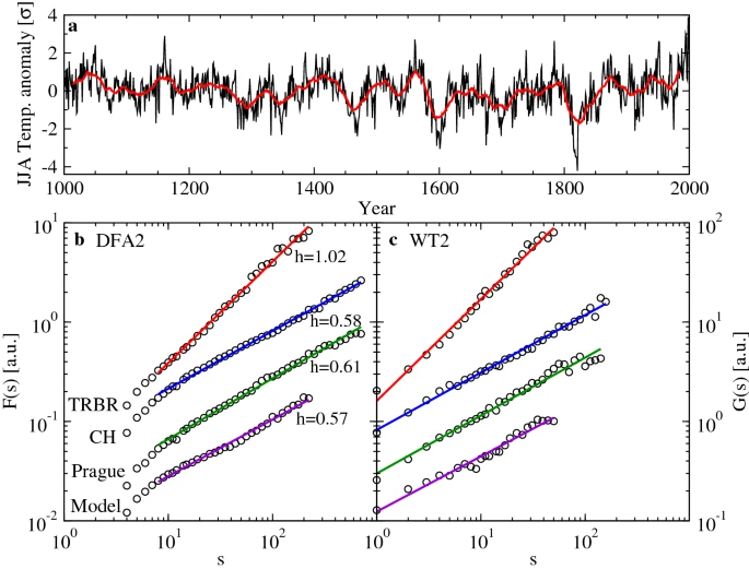
Tree ring-based reconstruction of the central European temperatures in the last millennium. a The reconstructed June-August temperatures in units of the records standard deviation. The red line depicts the moving average over 30 years. b, c The DFA2 fluctuation functions F(s) and the WT2 fluctuation functions G(s), respectively, for the reconstructed data from a, for monthly observational data (Swiss temperatures from Berkeley Earth, station data from Prague) and the MPI-ESM-P-past1000 model output for central European summer temperatures, from top to bottom. For the TRBR and model data, the time scale s is in years, while for the two observational records, it is in months. Note that in the double logarithmic presentation, the asymptotic slopes (Hurst exponents h) for the reconstruction data (\(h\cong 1\)) and the observational and model data (\(h\cong 0.6\)) differ strongly
2 Data and methods
2.1 Data
Tree-ring data: We consider the tree ring-based reconstruction (TRBR) of central European summer temperature variability by Büntgen et al. (2011), which reconstructs the June-August temperature over nearly the past 2500 years. A description of the methodology used can be found in Büntgen et al. (2011). The TRBR data set can be obtained from the NOAA paleoclimatology datasets (National Centers for Environmental Information). Here we focus on the last millennium, where also temperature reconstructions based on harvest dates are available. The data are displayed in Fig. 1a.
Harvest dates: The 4 harvest date records (Burgundy, Dijon and Swiss grape harvest data as well as rye harvest data) considered here specify, in each year, the calendar date where the harvest begins. From the records one can reconstruct the temperatures during the growth season in central Europe (Chuine et al. 2004; Labbé and Gaveau 2011; Meier et al. 2007; Wetter and Pfister 2011). (i) The Burgundy data set (Chuine et al. 2004) ranges from 1370 to 2003 and reconstructs the April–August temperatures. There exists one gap (1978) that we interpolated linearly. (ii) The French Dijon grape data set (Labbé and Gaveau 2011) is between 1385 and 1906 and represents the April-September temperatures. Since the Dijon data set has large gaps before 1448 we concentrated on the time span between 1448 and 1906. There are only short gaps that we filled by linear interpolation. (iii) The Swiss grape data set (Meier et al. 2007) is from the Swiss Plateau region and north-western Switzerland and ranges from 1480 to 2006 and reconstructs the April–August temperatures. (iv) The rye harvest data set (Wetter and Pfister 2011) is based on harvest dates in northern Switzerland and southwestern Germany. The data are between 1454 and 1970 and reconstruct the March–July temperatures.
Observational and model temperature data: We consider the long observational monthly temperature records for France and Switzerland that have been established by the Berkeley Earth analysis (Berkley Earth). The records range from 1753 to 2013. We also consider a long observational record from Prague (1775–2018) (Czech Hydrometeorological Institute). From the monthly data, we also obtain the mean June–August temperatures. Since these summer temperature time series are too short for a reliable DFA2 persistence analysis, which requires more than about 400 data points, we analyzed the complete monthly time series, which provide upper bounds for the seasonal Hurst exponents (see below). We also consider the central European summer temperatures from the output of the past 1000 (850–1849) run of the MPI-ESM-P general circulation earth system model (Jungclaus et al. 2010). We obtained the data from (Earth System Grid Federation).
2.2 Persistence analysis
It is well known that hydroclimatic records like temperature data and river flows are long-term persistent (Hurst 1951; Mandelbrot and Wallis 1969; Salas et al. 1980; Pelletier and Turcotte 1997; Koscielny-Bunde et al. 1998; Eichner et al. 2003; Koscielny-Bunde et al. 2006; Mudelsee 2007; Franzke 2010; Mudelsee 2013; Yuan and Fu 2014; Blesic et al. 2019; Yuan et al. 2019). The long-term persistence of temperature and river flow data represents an efficient testbed for model outputs, as well as reconstructions (Meko and Graybill 1995; Govindan et al. 2002; Livina et al. 2007; Ault et al. 2013).
In long-term persistent records \(\lbrace {y_i}\rbrace , i=1,\dots ,N\) with zero mean the power spectral density S(f) decays with increasing frequency f as \(S(f)\sim f^{-\beta }\) (see, e.g. Turcotte 1997). For white noise, \(\beta =0\). Records with \(0<\beta <1\) are stationary and can be characterized by an autocorrelation function C(s) with time lag s that decays by a power law, \(C(s)\sim (1-\gamma )s^{-\gamma }\), with \(\gamma =1-\beta\).
As a consequence of the long-term persistence, long-lasting deviations from the mean appear that lead to a characteristic mountain-valley structure in the record. With an increasing persistence, this mountain-valley structure becomes more pronounced, and the likelihood of encountering large mountains and deep valleys increases. Accordingly, it depends on the strength of the persistence, if a trend may be considered as natural or not (Lennartz and Bunde 2009b; Tamazian et al. 2015), and the prerequisite for comparing trends in different records is that both records have the same persistence characterized by the same \(\gamma\)-value.
Since both S(f) and C(s) exhibit large finite-size effects and are affected by external deterministic trends, one cannot use C(s) nor S(f) to reliably estimate the persistence of short records where N is of the order of \(10^3\). Here, to reveal the memory in the data, we followed (Bunde et al. 2013) and used wavelet (WT2) and detrended fluctuation analysis (DFA2), where fluctuation functions F(s) and G(s) are calculated. In long-term persistent data both fluctuation functions show power-law behavior \(\sim s^h\), \(h=(2-\gamma )/2\), but on complementary time scales s: WT2 on short time scales and DFA2 on longer time scales. For \(\gamma =1\) (white noise), \(h=1/2\).
Accordingly, the deviation of the (Hurst) exponent h from 1/2 quantifies the strength of the long-term persistence of a time series: h well above 1/2 signifies stronger long-term persistence with a pronounced mountain-valley structure, while \(h=1/2\) corresponds to white noise or short memory processes, e.g., an autoregressive process of first order, where the autocorrelation function decays exponentially. Thus, the question if an observed trend in a record is natural or not depends essentially on the Hurst exponent h of the record.
In both DFA2 and WT2 one measures the variability of a record by studying the fluctuations in segments of the record as a function of the segment length s. Accordingly, one first divides the record into non-overlapping windows \(\nu\) of lengths s.
In WT2 (see, e.g., Koscielny-Bunde et al. 1998; Bunde et al. 2013) one determines, in each segment \(\nu\), the mean value \(\bar{y}_{\nu }\) of the data and considers the linear combination \(\varDelta _\nu ^{(2)} = \bar{y}_{\nu }(s) - 2\bar{y}_{\nu +1}(s)+\bar{y}_{\nu +2}\). Then one averages \((\varDelta _\nu ^{(2)})^2\) over all segments \(\nu\), takes the square root and multiplies by s to arrive at the desired fluctuation function G(s). For white noise data, \(G(s)\sim s^{1/2}\). For long-term persistent records, we have
The exponent h can be associated with the Hurst exponent and is related to the correlation exponent \(\gamma\) and the spectral exponent \(\beta\) by \(h = 1-\gamma /2 = (1+\beta )/2\). For spectral exponents \(\beta\) above 1, corresponding to Hurst exponents above 1, the data are non stationary. A well-known example is a simple random walk, where \(\beta =2\) and \(h=1.5\).
In DFA2 (Kantelhardt et al. 2001) one focuses, in each segment \(\nu\), on the cumulated sum \(Y_i\) of the data and determines the variance \(F_{\nu }^2(s)\) of the \(Y_i\) around the best polynomial fit of order 2. After averaging \(F_{\nu }^2(s)\) over all segments \(\nu\) and taking the square root, we arrive at the desired fluctuation function F(s). One can show that for long-term persistent records,
Accordingly, F(s) and G(s) show the same power-law dependence on complementing time scales.By construction, linear (deterministic) trends in the data are eliminated, which is particularly important when determining long-term persistence in the presence of climate change. By evaluating both functions, we can measure long-term persistence from very short (\(s=1\)) towards very large (\(s=N/4\)) time scales.
We estimated the error bars for DFA2 and WT2 by creating long (\(N=2^{21}\)) synthetic records (Turcotte 1997) with prescribed Hurst exponents between \(h=0.2\) and \(h=1.5\) and analyzing by DFA2 and WT2 short subrecords with the same lengths as the original records. We identified the cases when the subrecords’ Hurst exponents were within \(\pm 0.01\) of the empirical (observational) data’s Hurst exponent and determined the distribution of the prescribed Hurst exponents, which correspond to these cases. The standard deviation of this distribution is taken as the error bar. For the shortest record (\(N=459\)) we obtain \(\varDelta h=0.06\), while for the longest record (\(N=3132\)) \(\varDelta h=0.03\).
For seasonal records comprised only of a subset of a year, e.g., summer temperatures June–August as in the tree-ring data or April–August as in the Burgundy data, the obtained Hurst exponent constitutes only a lower bound for the full years Hurst exponent. For an estimate of this effect, we have created synthetic full year records and analyzed the corresponding seasonal subrecords. For example, for the tree-ring data where \(N=1000\) and \(h=1.02\) the annual Hurst exponent is around \(h=1.1\), while for the Burgundy data with \(N=634\) and \(h=0.55\) the annual Hurst exponent is around \(h=0.64\).
We like to note that the Hurst exponent was first determined via a rescaled range (R/S) analysis (Hurst 1951) and is also referred to as Hurst coefficient. In a (R/S) analysis (for a review see, e.g., (Salas et al. 1980)) one considers how the range R of the cumulated sum Y, divided by the standard deviation of the data, scales with the considered segment length (period) s. For long-term persistent records, (R/S) scales as,
Compared with DFA2, drawbacks of the (R/S) analysis are (1) strong finite-size effects and (2) the dependence on external linear trends. DFA2 can also be generalized easily to study nonlinear correlations in a record (Kantelhardt et al. 2001).
3 Results
3.1 Long-term persistence
The result of the DFA2 and WT2 analysis of the tree ring-based summer temperatures of central Europe in the last millennium is shown in Fig. 1b, c. In the double logarithmic presentation, the asymptotic part of the DFA2 fluctuation function F(s) and the WT2 fluctuation function G(s) are straight lines, confirming the power-law behavior of F(s) and G(s), with slope \(h\cong 1.02\). Accordingly, the reconstructed temperature reveals a very high long-term persistence at the border towards non-stationarity. We compare this result with long monthly observational temperature records from Switzerland (1753–2013) and Prague (1775–2018) as well as with a long climate model simulation output (850–1849). For these records, the DFA2 analysis yields \(h=0.58, 0.61, 0.57\), respectively. The WT2 analysis yields \(h=0.58,0.58,0.56\), with the differences to the DFA2 analysis being within the error bars (\(\varDelta h\approx \pm 0.03\)). These values are consistent with numerous observational temperature records from the last century, where the Hurst exponent typically ranges between 0.55 and 0.75 (see, e.g., Koscielny-Bunde et al. 1998; Eichner et al. 2003). Thus the long-term persistence of the tree-ring data is considerably above the long-term persistence of the observational records.
However, since the observational data cover only a relatively short period, between 1753 and present, we cannot exclude a priori that the persistence of the central European temperatures might have changed over time or might depend on the regarded time scale, as suggested for precipitation records in Markonis and Koutsoyiannis (2016). To study this possibility, we expanded the time window by studying several harvest date based temperature reconstructions from central Europe, which go back up to 1370 (see Data and Methods section). Figure 2a–c show the graphs of the three harvest date proxy temperatures we considered. Figure 2d shows the negative harvest date anomalies for the Dijon grapes where a temperature reconstruction has not been performed. We include the Dijon record in our study since for the other 3 harvest data sets the negative harvest date anomalies and the reconstructed temperature anomalies based on them show the same structure, when the anomalies are plotted in units of their standard deviation from the mean. As in Fig. 1, the red curves denote the 30-year moving average revealing the long-term summer temperature variations. Figure 2e, f show the result of our DFA2 and WT2 persistence analysis. The figure shows that the fluctuation functions are characterized by Hurst exponents between \(h=0.52\) and \(h=0.69\), in agreement with the observational data and considerably below the tree-ring data.
3.2 Climate variations since 1753
For a more direct evaluation of the long-term summer temperature variations suggested by the tree-ring and harvest-date based proxies, we next compare the 30-year moving averages of the proxy data and the observed temperature records. For obtaining a coherent picture, before determining the moving average, we normalized each data set with respect to the period 1753–2000 by subtracting its mean and dividing by its standard deviation.

Harvest date based temperature reconstructions. Temperature anomalies based on a rye harvest dates from northern Switzerland and southwestern Germany (1454–1970), b grape harvest dates in Switzerland (1480–2006) and c grape harvest dates in Burgundy (1370–2003). d The inverted harvest date anomalies in Dijon (1385–1906). All anomalies are shown in units of their standard deviation from the mean. The red lines are moving averages over 30 years. e, f The DFA2 fluctuation functions F(s) (with Hurst exponents) and WT2 fluctuation functions G(s) of the records from (a–d). The WT2 Hurst exponents are \(h=0.59,0.63,0.54\) and 0.52 from top to bottom

Long-term summer temperature variations in Switzerland and France. 30-year moving averages of the observational temperatures (Berkeley Earth) of Switzerland (red), France (orange) and the temperature reconstructions based on tree rings (black), Swiss grape harvest dates (brown) and Burgundy harvest dates (blue). Note that the moving averages of both observational records are nearly identical; indeed, their correlation coefficient is close to 1
Figure 3 shows that between 1870 and 1988, the TRBR data reflect quite well (up to some offset) the observed long-term summer temperature variations, overestimating only slightly the depth of the valley around 1910. In this time window, the temperature reconstruction based on the tree rings appears to be superior to the harvest date based reconstructions. Between 1790 and 1870, however, the agreement is not so good. The TRBR curve runs through a valley as the observational curve does, but considerably exaggerates the depth of the valley. In contrast, the harvest date proxies only run through a shallow minimum, remarkably close to the observational data. The figure suggests that the TRBR data describes the appearance of warm and cold periods in the past properly, but, due to its considerably enhanced long-term persistence, overestimates the strengths of the cold and warm periods considerably.
3.3 Correction of the long-term persitence
To correct the enhanced long-term persistence in the TRBR, we are interested in a mathematical transformation of the data, which lowers the natural long-term persistence while leaving the gross features of the record, the positions of the warm and cold periods, unchanged. We performed the following mathematical transformation to change the original TRBR Hurst exponent \(h_0=1.03\) to \(h_1=0.60\) and thus to be in line with the observational, harvest and model data. Since this transformation is only suitable for altering a record’s natural long-term persistence, i.e., in the absence of external trends, we transformed the TRBR data between 1000 and 1990, before the current anthropogenic trend became relevant.
The transformation starts with calculating the Fourier transform \(y_0(f)\) of the TRBR data \(y_0(i)\). By definition, y(f) is related to the power spectrum S(f) by \(S(f)= \vert y(f)\vert ^2\sim f^{-(2h_0-1)}\). Next, we define \(y_1(f)=y_0(f) f^{(h_0-h_1)}\). Finally, we transform \(y_1(f)\) back to time space. The resulting record \(y_1(i)\) has the desired properties: It is long-term correlated with Hurst exponent \(h_1\) since its power spectrum scales as \(S_1(f)= \vert y_1(f)\vert ^2\sim \vert y_0(f)\vert ^2 f^{2(h_0-h_1)}\sim f^{-(2h_0-1)}f^{2(h_0-h_1)} \sim f^{-(2h_1-1)}\). This transformation reduces the height of warm periods and depths of cold periods but leaves their position unchanged.
Figure 4a compares the transformed TRBR data (blue) with \(h_1=0.6\) with the original TRBR data (black). The bold lines are the 30-year moving averages. The figure shows that by the transformation the structure of the original TRBR data is conserved, but the climate variations characterized by the depths of the minima and the heights of the maxima are reduced.

Original and transformed tree-ring proxy temperature record. a Compares the original TRBR record for the period 1000–1990, where the Hurst exponent h is 1.03 (black), with the transformed TRBR record, where \(h\equiv h_1=0.6\) (blue). For better visibility, the transformed TRBR record has been shifted downward by 5 units of its standard deviation. b How the magnitudes of the cold periods in the transformed TRBR record decrease with decreasing Hurst exponent \(h_1\). The magnitudes are quantified by the differences of the 30 year moving averages between the beginning and the end of the respective periods. c Compares the 30-year moving averages of the original and the transformed TRBR record (\(h=0.6\)) with the 30-year moving average of the observational temperatures from Switzerland. The comparison shows that the transformed TRBR record fits quite nicely with the observational data
To see how the strength of the long-term variations in the transformed TRBR data depends on their Hurst exponent \(h_1\), we have determined, in the 30-year moving average, the temperature differences in 4 periods (1415–1465, 1515–1536, 1562–1595, 1793–1824) where the greatest changes between 1350 and 1950 occur. The result is shown in Fig. 4b. The figure shows that the temperature difference between the beginning and the end of each period decreases continuously with decreasing h. For h around 0.6, the temperature differences are roughly halved.
Finally, we have compared the natural long-term variations in the transformed TRBR data with those in the observational data of Switzerland in the time interval between 1753 and 1990 (red curve) where anthropogenic effects have not yet become relevant. Figure 4c shows that the overall agreement between both data is very good, in particular in the period between 1790 and 1870, where the original TRBR data failed to reproduce the quite shallow minimum in the observational data. It is evident from Figs. 3 and 4c that the transformed TRBR curve fits best to both kinds of reconstructed and observed data, even though the period between 1870 and 1930 is not as well represented by the transformed TRBR data as the other periods. Interestingly, also the Burgundy and Swiss harvest data show a deviation in the same direction in this period.
4 Discussion
We suggest three possible reasons (or a combination thereof) for too much persistence in tree ring-based temperature reconstructions (i–iii): (i) If the applied standardization method, i.e., tree-ring detrending, is insufficient in removing all of the age-dependent biological growth trends, the resulting chronologies will be characterized by too much persistence. This methodological constraint will be strongest when using RCS-type detrending techniques on composite datasets for which samples are not randomly distributed over time. (ii) Since ring formation partly depends on previous year resources, carbon allocation from former year(s) results in too high persistence. (iii) Since tree growth always depends on soil moisture availability, inertia effects of soil property and water storage increase persistence. All of these factors (i–iii) are particularly strong when using ring width compared to wood density.
Our study is geographically limited to central Europe since long observational temperature records and long harvest date based temperature reconstructions are currently only available for this region. However, the analysis and, if necessary, the adjustment of a record’s long-term persistence is not limited to temperatures and generally applicable to other tree-ring based reconstructions of long-term persistent quantities, e.g., river flows.
In the case of streamflow reconstructions, the problem of persistence biases has gained a lot of attention, since the risk of multi-decadal droughts that can empty reservoirs, depends strongly on the assumed persistence properties (Ault et al. 2013, see also Woodhouse et al. 2006). So far, approaches to address persistence bias in this domain have been limited to short-term persistence. For instance, in Meko et al. (2001) the chronologies have been adjusted to have the same AR(1) coefficient as the observed streamflow.
In contrast, the mathematical transformation suggested here adjusts a record’s long-term persistence, to provide a more realistic reconstruction of the record’s low-frequency part, i.e., the climate variations characterized by, e.g., the 30-year moving average, but not of its high-frequency part. A simultaneous adjustment of a record’s long-term, as well as short-term persistence, might be achieved by a combined application of a fractional autoregressive integrated moving average (FARIMA) and an autoregressive integrated moving average (ARIMA) filtering. This remains for future work.
Since tree ring-based reconstructions play an important role in the understanding of past temperature variability, we suggest the use of the Hurst exponent as a standard practice to assess the reconstructions’ low-frequency properties and to compare the determined values with the Hurst exponents of other respective time series (observational, harvest dates, models). If deviations from the expected values are detected, the data should be transformed to adjust the Hurst exponent. This will lead to a more realistic reconstruction of the record’s low-frequency signal and thus to a better understanding of the climate variations of the past.
References
Ault TR, Cole JE, Overpeck JT, Pederson GT, George SS, Otto-Bliesner B, Woodhouse CA, Deser C (2013) The continuum of hydroclimate variability in western North America during the last millennium. J Clim 26:5863–5878
Berkeley Earth. http://berkeleyearth.org/. Accessed 29 Jan 2019
Blesić S, Zanchettin D, Rubino A (2019) Heterogeneity of scaling of the observed global temperature data. J Clim 32:349–367
Bunde A, Kropp J, Schellnhuber HJ (eds) (2012) The science of disasters: climate disruptions, heart attacks, and market crashes. Springer, Berlin
Bunde A, Büntgen U, Ludescher J, Luterbacher J, von Storch H (2013) Is there memory in precipitation? Nat Clim Change 3:174–175
Büntgen U, Tegel W, Nicolussi K, McCormick M, Frank D, Trouet V, Kaplan JO, Herzig F, Heussner K, Wanner H, Luterbacher J, Esper J (2011) 2500 years of European climate variability and human susceptibility. Science 331:578–582
Chuine I, Yiou P, Viovy N, Seguin B, Daux V, Le Roy Ladurie E (2004) Grape ripening as a past climate indicator. Nature 432:289–290
Cook ER, Meko DM, Stahle DW, Cleaveland MK (1999) Drought reconstructions for the continental United States. J Clim 12:1145–1162
Czech Hydrometeorological Institute, Prague Clementinum. http://portal.chmi.cz/historicka-data/pocasi/praha-klementinum?l=en. Accessed 29 Jan 2019
Earth System Grid Federation. https://esgf-data.dkrz.de/projects/esgf-dkrz/. Accessed 29 Jan 2019
Eichner JF, Koscielny-Bunde E, Bunde A, Havlin S, Schellnhuber HJ (2003) Power-law persistence and trends in the atmosphere: a detailed study of long temperature records. Phys Rev E 68:046133
Esper J, Krusic PJ, Ljungqvist FC, Luterbacher J, Carrer M, Cook E, Davi NK, Hartl-Meier C, Kirdyanov A, Konter O, Myglan V, Timonen M, Treydte K, Trouet V, Villalba R, Yang B, Büntgen U (2016) Ranking of tree-ring based temperature reconstructions of the past millennium. Quat Sci Rev 145:134–151
Franke J, Frank D, Raible CC, Esper J, Brönnimann S (2013) Spectral biases in tree-ring climate proxies. Nat Clim Change 3:360–364
Franzke C (2010) Long-range dependence and climate noise characteristics of Antarctic temperature data. J Clim 23:6074–6081
Govindan RB, Vyushin D, Bunde A, Brenner S, Havlin S, Schellnhuber HJ (2002) Global climate models violate scaling of the observed atmospheric variability. Phys Rev Lett 89:028501
Hurst HE (1951) Long Term storage capacity of reservoirs. Trans Am Soc Civ Eng 116:770–799
Jungclaus JH, Lorenz SJ, Timmreck C, Reick CH, Brovkin V, Six K, Segschneider J, Giorgetta MA, Crowley TJ, Pongratz J, Krivova NA, Vieira LE, Solanki SK, Klocke D, Botzet M, Esch M, Gayler V, Haak H, Raddatz TJ, Roeckner E, Schnur R, Widmann H, Claussen M, Stevens B, Marotzke J (2010) Climate and carbon-cycle variability over the last millennium. Clim Past 6:723–737
Kantelhardt JW, Koscielny-Bunde E, Rego HHA, Havlin S, Bunde A (2001) Detecting long-range correlations with detrended fluctuation analysis. Phys A 295:441–454
Koscielny-Bunde E, Bunde A, Havlin S, Roman E, Goldreich Y, Schellnhuber HJ (1998) Indication of a universal persistence law governing atmospheric variability. Phys Rev Lett 81:729–732
Koscielny-Bunde E, Kantelhardt JW, Braun P, Bunde A, Havlin S (2006) Long-term persistence and multifractality of river runoff records: detrended fluctuation studies. J Hydrol 322:120–137
Labbé T, Gaveau F (2011) The dates of bann harvest in Dijon: critical establishment and archive revision of an old series. Revue Historique 657:19–51
Lennartz S, Bunde A (2009a) Eliminating finite-size effects and detecting the amount of white noise in short records with long-term memory. Phys Rev E 79:066101
Lennartz S, Bunde A (2009b) Trend evaluation in records with long-term memory: application to global warming. Geophys Res Lett 36:L16706
Livina V, Kizner Z, Braun P, Molnar T, Bunde A, Havlin S (2007) Temporal scaling comparison of real hydrological data and model runoff records. J Hydrol 36:186–198
Mandelbrot BB, Wallis JR (1969) Some long-run properties of geophysical records. Water Resour Res 5(2):321–340
Markonis Y, Koutsoyiannis D (2016) Scale-dependence of persistence in precipitation records. Nat Clim Change 6:399–401
Matalas NC (1962) Statistical properties of tree ring data. Hydrol Sci J 7:39–47
Matsoukas C, Islam S, Rodriguez-Iturbe I (2000) Detrended fluctuation analysis of rainfall and streamflow time series. J Geophys Res Atmos 105(D23):29165–29172
Meier N, Rutishauser T, Pfister C, Wanner H, Luterbacher J (2007) Grape harvest dates as a proxy for Swiss April to August temperature reconstructions back to AD 1480. Geophys Res Lett 34:L20705
Meko D, Graybill DA (1995) Tree-ring reconstruction of Upper Gila River discharge. J Am Water Resour Assoc 31:605–616
Meko DM, Therrell MD, Baisan CH, Hughes MK (2001) Sacramento River flow reconstructed to A.D. 869 from tree rings. J Am Water Resour Assoc 37:1029–1039
Moberg A (2012) Comments on reconstruction of the extra-tropical NH mean temperature over the last millennium with a method that preserves low-frequency variability. J Clim 25:7991–7997
Mudelsee M (2007) Long memory of rivers from spatial aggregation. Water Resour Res 43:W01202
Mudelsee M (2013) Climate time series analysis. Springer, Heidelberg
National Centers for Environmental Information, Paleoclimatology Datasets. https://www.ncdc.noaa.gov/data-access/paleoclimatology-data/datasets. Accessed 29 Jan 2019
Pelletier JD, Turcotte DL (1997) Long-range persistence in climatological and hydrological time series: Analysis, modeling and application to drought hazard assessment. J Hydrol 203:198–208
Salas JD, Delleur JW, Yevjevich V, Lane WL (1980) Applied modeling of hydrologic time series. Water Resources Publications Highlands, Ranch
Stocker TF, Qin D, Plattner GK, Tignor M, Allen SK, Boschung J, Nauels A, Xia Y, Bex V, Midgley PM (eds) (2013) Climate change 2013: the physical science basis. A report of Working Group I of the Intergovernmental Panel on Climate Change. Cambridge University Press, Cambridge
Tamazian A, Ludescher J, Bunde A (2015) Significance of trends in long-term correlated records. Phys Rev E 91:032806
Turcotte DL (1997) Fractals and chaos in geology and geophysics. Cambridge University Press, Cambridge
von Storch H, Zorita E, Jones JM, Dimitriev Y, González-Rouco F, Tett SFB (2004) Reconstructing past climate from noisy data. Science 306:679–682
Vyushin D, Zhidkov I, Havlin S, Bunde A, Brenner S (2004) Volcanic forcing improves atmosphere-ocean coupled general circulation model scaling performance. Geophys Res Lett 31:L10206
Wetter O, Pfister C (2011) Spring-summer temperatures reconstructed for northern Switzerland and southwestern Germany form the winter rye harvest dates 1454–1970. Clim Past 7:1307–1326
Woodhouse CA, Gray ST, Meko DM (2006) Updated streamflow reconstructions for the Upper Colorado River Basin. Water Resour Res. https://doi.org/10.1029/2005WR00445
Yuan N, Fu Z (2014) Century-Scale Intensity Modulation of Large-Scale Variability in Long Historical Temperature Records. J Clim 27:1742–1750
Yuan N, Huang Y, Duan J, Zhu C, Xoplaki E, Luterbacher J (2019) On climate prediction: how much can we expect from climate memory? Clim Dyn 52:855–864
Acknowledgements
J. L. thanks for the support by the East Africa Peru India Climate Capacities (EPICC) project. This project is part of the International Climate Initiative (IKI) of the Federal Ministry for the Environment, Nature Conservation and Nuclear Safety (BMU).
Funding
Open Access funding provided by Projekt DEAL.
Author information
Authors and Affiliations
Corresponding author
Additional information
Publisher's Note
Springer Nature remains neutral with regard to jurisdictional claims in published maps and institutional affiliations.
Rights and permissions
Open Access This article is licensed under a Creative Commons Attribution 4.0 International License, which permits use, sharing, adaptation, distribution and reproduction in any medium or format, as long as you give appropriate credit to the original author(s) and the source, provide a link to the Creative Commons licence, and indicate if changes were made. The images or other third party material in this article are included in the article's Creative Commons licence, unless indicated otherwise in a credit line to the material. If material is not included in the article's Creative Commons licence and your intended use is not permitted by statutory regulation or exceeds the permitted use, you will need to obtain permission directly from the copyright holder. To view a copy of this licence, visit http://creativecommons.org/licenses/by/4.0/.
About this article

Cite this article
Ludescher, J., Bunde, A., Büntgen, U. et al. Setting the tree-ring record straight. Clim Dyn 55, 3017–3024 (2020). https://doi.org/10.1007/s00382-020-05433-w
Received:
Accepted:
Published:
Issue Date:
DOI: https://doi.org/10.1007/s00382-020-05433-w