A general account of coinduction up-to

Abstract

Bisimulation up-to enhances the coinductive proof method for bisimilarity, providing efficient proof techniques for checking properties of different kinds of systems. We prove the soundness of such techniques in a fibrational setting, building on the seminal work of Hermida and Jacobs. This allows us to systematically obtain up-to techniques not only for bisimilarity but for a large class of coinductive predicates modeled as coalgebras. The fact that bisimulations up to context can be safely used in any language specified by GSOS rules can also be seen as an instance of our framework, using the well-known observation by Turi and Plotkin that such languages form bialgebras. In the second part of the paper, we provide a new categorical treatment of weak bisimilarity on labeled transition systems and we prove the soundness of up-to context for weak bisimulations of systems specified by cool rule formats, as defined by Bloom to ensure congruence of weak bisimilarity. The weak transition systems obtained from such cool rules give rise to lax bialgebras, rather than to bialgebras. Hence, to reach our goal, we extend the categorical framework developed in the first part to an ordered setting.

1 Introduction

1.1 Coinduction up-to

The rationale behind coinductive up-to techniques is the following. Suppose you have a characterisation of an object of interest as a greatest fixed-point. For instance, behavioural equivalence in CCS is the greatest fixed-point of a monotone function B on relations, describing the standard bisimulation game. This means that to prove two processes equivalent, it suffices to exhibit a relation R that relates them, and which is a B-invariant, i.e., $R\subseteq B(R)$. However, such a task may be cumbersome or inefficient, and one might prefer to exhibit a relation which is only a B-invariant up to some function A, i.e., $R\subseteq B(A(R))$.

Not every function A can safely be used: A should be sound for B, meaning that any B-invariant up to A should be contained in a B-invariant. Instances of sound functions for behavioural equivalence in process calculi usually include transitive closure, contextual closure and congruence closure. The use of such techniques dates back to Milner’s work on CCS [34]. A famous example of an unsound technique is that of weak bisimulation up to weak bisimilarity. Since then, coinduction up-to proved useful, if not essential, in numerous proofs about concurrent systems (see [41] for a list of references); it has been used to obtain decidability results [16], and more recently to improve standard automata algorithms [12].

The theory underlying these techniques was first developed by Sangiorgi [45]. It was then reworked and generalised by one of the authors to the abstract setting of complete lattices [40, 41]. The key observation there, is that the notion of soundness is not compositional: the composition of two sound functions is not necessarily sound itself. The main solution to this problem consists in restricting to compatible functions, a subset of the sound functions which enjoys nice compositionality properties and contains most of the useful techniques.

An illustrative example of the benefits of a modular theory is the following: given a signature ${\varSigma }$, consider the congruence closure function, that is, the function $Cgr$ mapping a relation R to the smallest congruence containing R. This function has proved to be useful as an up-to technique for language equivalence of non-deterministic automata [12]. It can be decomposed into small pieces as follows: $Cgr = Trn \circ Sym \circ Ctx \circ Rfl$, where $Trn$ is the transitive closure, $Sym$ is the symmetric closure, $Rfl$ is the reflexive closure, and $Ctx$ is the context closure associated to ${\varSigma }$. Since compatibility is preserved by composition (among other operations), the compatibility of $Cgr$ follows from that of its smaller components. In turn, transitive closure can be decomposed in terms of relational composition, and contextual closure can be decomposed in terms of the smaller functions that close a relation with respect to ${\varSigma }$ one symbol at a time. Compatibility of these functions can thus be obtained in a modular way.

A key observation in the present work is that when we move to a coalgebraic presentation of the theory, compatible functions generalise to functors equipped with a distributive law (Sect. 3).

1.2 Fibrations and coinductive predicates

Coalgebras are our tool of choice for describing state based systems: given a functor F determining its type (e.g., labeled transition systems, automata, streams), a system is just an F-coalgebra $(X,\xi )$. When F has a final coalgebra $({\varOmega },\omega )$, this gives a canonical notion of behavioural equivalence [27]:

two states $x,y\in X$ are equivalent if they are mapped to the same element in the final coalgebra.

When the functor F preserves weak pullbacks—which we shall assume throughout this introductory section for the sake of simplicity—behavioural equivalence can be characterised coinductively using Hermida–Jacobs bisimulations [23, 51]: given an F-coalgebra $(X,\xi )$, behavioural equivalence is the largest B-invariant for a monotone function B on $\mathsf {Rel}_X$, the poset of binary relations over X. This function B can be decomposed as

$$\begin{aligned} B~\triangleq ~\xi ^*\circ \mathsf {Rel}(F)_X:\mathsf {Rel}_X\rightarrow \mathsf {Rel}_X \end{aligned}$$

Let us explain the notations used here. We consider the category $\mathsf {Rel}$ whose objects are relations $R \subseteq X^2$ and morphisms from $R \subseteq X^2$ to $S \subseteq Y^2$ are maps from X to Y sending pairs in R to pairs in S. For each set X the poset $\mathsf {Rel}_X$ of binary relations over X is a subcategory of $\mathsf {Rel}$, also called the fibre over X. The functor F has a canonical lifting to $\mathsf {Rel}$, denoted by $\mathsf {Rel}(F)$. This lifting restricts to a functor $\mathsf {Rel}(F)_X :\mathsf {Rel}_X \rightarrow \mathsf {Rel}_{FX}$, which in this case is just a monotone function between posets. The monotone function $\xi ^* :\mathsf {Rel}_{FX} \rightarrow \mathsf {Rel}_X$ is the inverse image of the coalgebra $\xi$, mapping a relation $R \subseteq (FX)^2$ to $(\xi \times \xi )^{-1}(R)$.

To express other predicates than behavioural equivalence, one can take arbitrary liftings of F to $\mathsf {Rel}$, different from the canonical one. Any lifting $\overline{F}$ yields a functor B defined as

$$\begin{aligned} B~\triangleq ~\xi ^*\circ \overline{F}_X:\mathsf {Rel}_X\rightarrow \mathsf {Rel}_X \qquad \qquad \qquad \qquad \qquad \qquad \qquad \qquad \,\,\,\, \qquad \qquad \qquad \qquad \qquad \qquad (\dagger ) \end{aligned}$$

The final coalgebra, or greatest fixed-point for such a B is called a coinductive predicate [22, 23]. Considering appropriate liftings $\overline{F}$, one obtains, for instance, various behavioural preorders: similarity on labeled transition systems (LTSs), language inclusion on automata, or lexicographic ordering of streams.

This situation can be further generalised using fibrations. We refer the reader to the first chapter of [26] for a gentle introduction, but Sect. 4 provides all the definitions required for the understanding of our results. The running example of a fibration is the functor $p :\mathsf {Rel}\rightarrow \mathsf {Set}$ mapping a relation $R\subseteq X^2$ to its support set X, see Sect. 4. In this fibration, the inverse image $\xi ^*$ is the reindexing functor of $\xi$.

By choosing a different fibration than $\mathsf {Rel}$, one can obtain coinductive characterisations of objects that are not necessarily binary relations, e.g., unary predicates like divergence, ternary relations, or metrics.

Our categorical generalisation of compatible functions provides a natural extension of this fibrational framework with a systematic treatment of up-to techniques: we provide functors (i.e., monotone functions in the special case of the $\mathsf {Rel}$ fibration) that are compatible with those functors B corresponding to coinductive predicates.

For instance, when the chosen lifting $\overline{F}$ is a fibration map, the functor corresponding to a technique called “up to behavioural equivalence” is compatible (Theorem 6.1). The canonical lifting of a functor is always such a fibration map, so that when F is the functor for LTSs, we recover the soundness of the first up-to technique introduced by Milner, namely “bisimulation up to bisimilarity” [34]. One can also check that another lifting of this same functor but in another fibration yields the divergence predicate, and is a fibration map. We thus obtain the validity of the “divergence up to bisimilarity” technique.

1.3 Bialgebras and up to context

Another important class of techniques comes into play when considering systems with an algebraic structure on the state space (e.g., the syntax of a process calculus). A minimal requirement for such systems usually is that behavioural equivalence should be a congruence. In the special case of bisimilarity on LTSs, several rule formats have been proposed to ensure such a congruence property [1]. At the categorical level, the main concept to study such systems is that of bialgebras. Assume two endofunctors T, F related by a distributive law $\lambda :TF\Rightarrow FT$. A $\lambda$-bialgebra is a triple $(X,\alpha ,\xi )$ consisting of a T-algebra $(X,\alpha )$ and an F-coalgebra $(X,\xi )$, compatible in the sense that a certain diagram involving $\lambda$ commutes. It is well known that in such a bialgebra, behavioural equivalence is a congruence with respect to T [54]. This is actually a generalisation of the fact that bisimilarity is a congruence for all GSOS specifications [6]: GSOS specifications are in one-to-one correspondence with distributive laws between the appropriate functors [4, 54].

This congruence result can be strengthened into a compatibility result [43]: in any $\lambda$-bialgebra, the contextual closure function that corresponds to T is compatible for behavioural equivalence. However [43] deals only with the canonical relational liftings. Using fibrations, we generalise this result to arbitrary liftings, both on the coalgebraic and on the algebraic side. Using other fibrations than $\mathsf {Rel}$ we obtain up to context techniques for arbitrary coinductive predicates, e.g., for unary predicates like divergence. Our framework also encompasses other relations than behavioural equivalence, like the behavioural preorders mentioned above.

The technical device we need to establish this result is that of bifibrations, fibrations p whose opposite functor $p^ op$ is also a fibration. We keep the running example of the $\mathsf {Rel}$ fibration for the sake of clarity; the results are presented in full generality in the remaining parts of the paper. In such a setting, any morphism $f:X\rightarrow Y$ in $\mathsf {Set}$ has a direct image $\coprod _f :\mathsf {Rel}_X\rightarrow \mathsf {Rel}_Y$. Now given an algebra $\alpha :TX\rightarrow X$ for a functor T on $\mathsf {Set}$, any lifting $\overline{T}$ of T gives rise to a functor on the fibre above X, defined dually to $(\dagger )$:

When we take for $\overline{T}$ the canonical lifting of T in $\mathsf {Rel}$, then C is the contextual closure function corresponding to the functor T. We shall see that we sometimes need to consider variations of the canonical lifting to obtain a compatible up-to technique (e.g., up to “monotone” contexts for checking language inclusion of weighted automata—Sect. 8.1).

Now, starting from a $\lambda$-bialgebra $(X,\alpha ,\xi )$, and given two liftings $\overline{T}$ and $\overline{F}$ of T and F, respectively, the question is whether the above functor C is compatible with the functor B defined earlier in $(\dagger )$. The simple condition we give in this paper is the following: the distributive law $\lambda :TF\Rightarrow FT$ should lift to a distributive law $\overline{\lambda }:\overline{T}\,\overline{F}\Rightarrow \overline{F}\,\overline{T}$ (Theorem 6.7).

This condition is always satisfied in the bifibration $\mathsf {Rel}$, when $\overline{T}$ and $\overline{F}$ are the canonical liftings of T and F. Thus we obtain as a corollary the compatibility of bisimulation of up to context in $\lambda$-bialgebras, which is the main result from [43] and appeared in a slightly different form in [33]—soundness was previously observed by Lenisa et al. [31, 32] and then Bartels [4].

1.4 Contributions and applications

The main contributions of this paper are as follows. Firstly, Sect. 6 develops an abstract framework for proving soundness of up-to techniques. Secondly, this allows us to derive the soundness of a wide range of both novel and well-established up-to techniques for arbitrary coinductive predicates. These results are summarised in two tables in Sect. 6.4 and illustrated by examples in Sect. 8. We further extend our results in Sect. 7 to deal with abstract GSOS specifications [29, 54]. Thirdly, in the second part of the paper (Sects. 10–13) we extend our theoretical framework to an ordered setting, to provide up-to techniques for weak bisimulations and simulations.

In Sect. 8.2 we prove the compatibility of a novel technique called “divergence up to behavioural equivalence and left contextual closure”. In this example we use the predicate fibration on $\mathsf {Set}$ that, in general, is suitable to characterise formulas from modal logic as coinductive predicates. (See [17] for an account of coalgebraic modal logic.) One can also change the base category: by considering the fibration of equivariant relations over nominal sets, we show how to obtain up-to techniques for language equivalence of non-deterministic nominal automata [7]. In Sect. 8.3, these techniques allow us to prove the equivalence of two nominal automata using an orbit-finite relation, where the standard method would require an infinite one (recall that the determinisation of a nominal automaton is not necessarily orbit-finite).

The second part of this paper deals with other applications for which an ordered setting is required. The main motivation comes from weak bisimilarity, a behavioural equivalence allowing to abstract over internal transitions, labeled with the special action $\tau$. When the player proposes a transition $\mathop {\rightarrow }\limits ^{a}$, the opponent must answer with a saturated transition $\mathop {\Rightarrow }\limits ^{a}$, which is roughly a transition $\mathop {\rightarrow }\limits ^{a}$ possibly combined with internal actions $\mathop {\rightarrow }\limits ^{\tau }$. This slight dissymmetry results in a much more delicate theory of up-to techniques. For instance, up-to weak bisimilarity and up-to transitive closure are no longer sound for weak bisimulations. And up-to context has to be restricted: the external choice from CCS cannot be freely used [46].

The results we prove in Sects. 6 and 7 require bialgebras and, unfortunately, the saturated transition system does not form a bialgebra. Intuitively, in a bialgebra all and only the transitions of a composite system can be derived from transitions of its components. For the saturated transition relation $\Rightarrow$, one implication fails: a composite system performs weak transitions which are not derived from transitions of its components (see Example 9.2). But the other implication holds, which is made precise by the observation that the saturated transition relation gives rise to a so-called lax bialgebra. This is the key observation that leads to the rather involved refinement we propose in Sect. 10. This allows us to prove in Sect. 11 that up-to context is compatible for lax models of positive GSOS specifications [1] and thus to obtain in Sect. 12 the soundness of up-to context for weak bisimulations in systems specified by the cool rule format from [55].

Finally, in Sect. 13 we consider up-to techniques for similarity. Using the coalgebraic presentation of similarity in terms of lax relation lifting, (see, e.g., [25]) and the infrastructure developed in Sect. 11, we obtain that “up to context” is compatible whenever we start from a monotone distributive law. In the special case of LTSs, this monotonicity condition amounts to the positive GSOS rule format [20]: GSOS without negative premises.

Previous work This paper is an extended version of [10] and [11]. We extended the previous works with careful explanations and detailed proofs, three motivating examples (Sect. 2) and several side results (such as those in Sects. 3.1 and 7).

Outline We present motivating examples in Sect. 2. Then we introduce coinduction and up-to techniques in a categorical setting (Sect. 3), before recalling the basic definitions of fibrations (Sect. 4) and coinductive predicates (Sect. 5). The main results are developed in Sect. 6, where we obtain up-to techniques in a fibrational setting. Sect. 7 is devoted to technical results allowing to import tools from abstract GSOS specifications. At this point we give several examples of our theory at work (Sect. 8). Then we explain the difficulties that arise with weak bisimulation in Sect. 9, which motivates an extension of our framework to an ordered setting (Sect. 10). In Sect. 11 we come back to abstract GSOS specifications in the ordered setting, before dealing with weak bisimulation in Sect. 12, and simulation in Sect. 13. We conclude with directions for future work in Sect. 14. For the sake of clarity, we postponed many proofs to the appendices, whose structure follows that of the main text.

2 Motivating examples

Before starting the main technical development, we present three motivating examples where we provide a coinductive perspective on some classical results of automata theory. First, we recall the basic notions of deterministic automaton, bisimulation and coinduction in a lattice theoretic setting.

A deterministic automaton on the alphabet A is a pair $(X,\langle o,t\rangle )$, where X is a set of states and $\langle o,t\rangle :X \rightarrow 2\times X^A$ is a function with two components: o, the output function, determines if a state x is final ($o(x) = 1$) or not ($o(x) = 0$); and t, the transition function, returns for each input letter $a \in A$ the next state.

Every automaton $(X,\langle o,t\rangle )$ induces a function $[\![ - ]\!]:X \rightarrow 2^{A^*}$ mapping each state of the automaton to the language that it accepts. Formally this function is defined for all $x\in X$, $a \in A$ and $w\in A^*$ as follows.

$$\begin{aligned}{}[\![ x ]\!](\varepsilon )= & {} o(x) \\ [\![ x ]\!](aw)= & {} [\![ t(x)(a) ]\!](w) \end{aligned}$$

Two states $x,y\in X$ are said to be language equivalent, in symbols $x \sim y$, iff $[\![ x ]\!]=[\![ y ]\!]$. Alternatively, language equivalence can be defined coinductively as the greatest fixed-point of a function B on $\mathsf {Rel}_X$, the lattice of relations over X. For all $R\subseteq X^2$, $B:\mathsf {Rel}_X \rightarrow \mathsf {Rel}_X$ is defined as

$$\begin{aligned} B(R)=\{(x,y) \mid o(x)=o(y) \text { and for all } a\in A, \, (t(x)(a), t(y)(a))\in R\}. \end{aligned}$$

Indeed, one can check that B is monotone and that the greatest fixed-point of B, hereafter denoted by $\nu B$, coincides with $\sim$. A post fixed-point of B, i.e., a relation $R\subseteq B(R)$, is called a bisimulation.

The Knaster-Tarski fixed-point theorem characterises $\nu B$ as the union of all post-fixed points of B:

$$\begin{aligned} \nu B= \bigcup \{ R \subseteq X^2 \mid R \subseteq B(R) \}. \end{aligned}$$

This immediately leads to the coinduction proof principle

(1)

which allows to prove $x \sim y$ by exhibiting a bisimulation R such that $\{(x,y)\} \subseteq R$.

For an example of a bisimulation, consider the following deterministic automaton, where final states are overlined and the transition function is represented by labeled arrows. The relation consisting of dashed and dotted lines is a bisimulation witnessing, for instance, that $x\sim u$.

2.1 Hopcroft and Karp’s algorithm

The famous algorithm by Hopcroft and Karp for checking language equivalence [24] relies on coinduction implicitly, long before Milner’s pioneering work on bisimulation. Hopcroft and Karp actually use coinduction up to equivalence closure. Consider the function $Eqv :\mathsf {Rel}_X \rightarrow \mathsf {Rel}_X$ mapping every relation $R\subseteq X^2$ to its equivalence closure. A bisimulation up to $Eqv$ is a relation R such that

$$\begin{aligned} R\subseteq B ( Eqv (R)). \end{aligned}$$

For example, consider the automaton above and the relation R containing only the dashed lines: since $t(x)(b)=y$, $t(u)(b)=w$ and $(y,w)\notin R$, then $(x,u)\notin B(R)$. This means that R is not a bisimulation; however it is a bisimulation up to $Eqv$, since (y, w) belongs to $Eqv (R)$ and (x, u) to $B( Eqv (R))$.

In general, bisimulations up-to can be smaller than plain bisimulation and this feature can have a relevant impact in the performance of algorithms for checking language equivalence. A naive version of Hopcroft and Karp’s algorithm that does not use up-to equivalence might have to explore $n^2$ pairs of states (where n is the number of states) while, by exploiting this technique, Hopcroft and Karp’s algorithm visits at most n pairs (that is the number of equivalence classes). The case of non-deterministic automata is even more impressive: another up-to technique, called up-to congruence, allows for an exponential improvement on the performance of algorithms for checking language equivalence [12]. In Sect. 8.3, we will provide an example of bisimulation up-to congruence in the setting of non-deterministic nominal automata.

2.2 Regular expressions and Kleene algebra

Beyond algorithms, up-to techniques are useful to prove different sorts of properties of systems specified by a given syntax. Indeed, this was the original motivation for the introduction of up-to techniques in Milner’s work on CCS [34]. To keep the presentation simpler and, at the same time, to show to the reader the large spectrum of applications of up-to techniques, we consider regular expressions and we provide coinductive proofs for some of the axioms of Kleene Algebra [30] with respect to the regular language interpretation.

First, recall that regular expressions are generated by the following grammar

$$\begin{aligned} e::= 0 \mid 1 \mid a \mid e+e \mid e\cdot e \mid e^\star \end{aligned}$$

where a ranges over symbols of the alphabet A. To make the notation lighter we will often avoid to write $\cdot$, so that ef stands for $e \cdot f$.

We will prove language equivalence of regular expressions by considering bisimulations on an automaton having as state space the set RE of regular expressions. This automaton is constructed using Brzozowski derivatives [15]. The following inference rules

define the output function $o :RE \rightarrow 2$ as $o(e) = 1$ iff $e{\downarrow }$. The following inference rules

define the transition function $t:RE\rightarrow RE^A$ as $t(e)(a)=e'$ iff $e\mathop {\rightarrow }\limits ^{a}e'$. The above presentation of Brzozowski derivatives by means of inference rules is unusual, but it is convenient here to stress the similarity with GSOS specifications [6] that will be pivotal for our development in Sect. 7.

The deterministic automaton $(RE,\langle o,t\rangle )$ uniquely defines the map $[\![ - ]\!]:RE \rightarrow 2^{A^\star }$ and Kleene Algebra provides a sound and complete axiomatisation for $\sim$. The soundness of these axioms can be now proved by means of coinduction. For instance, commutativity of $+$,

$$\begin{aligned} e+f \sim f+e \end{aligned}$$

is simply proved by checking that the relation $R=\{(e+f,f+e) \mid e,f\in RE \}$ is a bisimulation. Indeed $(e+f){\downarrow } \Leftrightarrow e{\downarrow } \vee f{\downarrow } \Leftrightarrow (f+e){\downarrow }$ and for all $a\in A$,

In a similar way, one can prove that $(RE,+,0)$ is a monoid, but things get trickier for distributivity, for instance on the right:

$$\begin{aligned} e(f+g)\sim ef + eg. \end{aligned}$$

Indeed, let us check whether the relation $R=\{(e(f+g), ef + eg) \mid e,f,g\in RE \}$ is a bisimulation. It is immediate to check that $e(f+g){\downarrow } \Leftrightarrow (ef + eg){\downarrow }$. However, the arriving states after a transition are not related by R, hence R is not a bisimulation.

(2)

However, as we will see below, the relation R is a bisimulation up-to for a particular composite up-to technique. Its components are the function $Bhv :\mathsf {Rel}_{RE} \rightarrow \mathsf {Rel}_{RE} \rightarrow \mathsf {Rel}_{RE}$ defined for all relations $R\subseteq RE^2$ as

$$\begin{aligned} Bhv (R)= \{(e,f)\mid \exists e',f' \text { s.t. } e \sim e' R f' \sim f \} \end{aligned}$$

and the function $Ctx :\mathsf {Rel}_{RE} \rightarrow \mathsf {Rel}_{RE}$ mapping every relation R to its contextual closure $Ctx (R)$. The latter is defined inductively by the following rules.

Now, it is easy to see that the relation $R=\{(e(f+g), ef + eg) \mid e,f,g\in RE \}$ is a bisimulation up to $Bhv \circ Ctx$, meaning that $R\subseteq B ( Bhv ( Ctx (R)))$. Indeed (2) is proved to hold by observing that

$$\begin{aligned} e'(f+g)+o(e)(f'+g') \mathrel { Ctx (R)} (e'f+e'g) +(o(e)f'+o(e)g') \end{aligned}$$

and that $(e'f+e'g) +(o(e)f'+o(e)g') \sim (e'f +o(e)f') + (e'g +o(e)g')$ since, as shown above, $+$ is associative and commutative. Hence, the arriving states in (2) are related by $Bhv \circ Ctx (R)$.

2.3 Arden’s rule

As the last example of this section, we provide a coinductive proof of Arden’s rule. This is usually formulated for arbitrary languages, but we rephrase it here in terms of regular expressions so to reuse the notation introduced so far. The coinductive proof for arbitrary languages is completely analogous, see [42].

Arden’s rule states that, given two expressions k and m, the “behavioural” equation

$$\begin{aligned} e \sim k e+m \end{aligned}$$

has $e=k^\star m$ as solution, i.e., $k^\star m \sim k k^\star m +m$. Furthermore,

• (a) it is the smallest solution (up to $\sim$), namely if $f \sim k f+m$ then $k^\star m \precsim f$;

• (b) if , then it is the unique solution (up to $\sim$), namely if $f \sim k f+m$ then $k^\star m \sim f$.

Here $\precsim$ denotes language inclusion: $e \precsim f$ iff $[\![ e ]\!]\subseteq [\![ f ]\!]$. In order to proceed with a coinductive proof of Arden’s rule, we characterise $\precsim$ as $\nu B'$, the greatest fixed-point of the monotone function $B' :\mathsf {Rel}_{RE} \rightarrow \mathsf {Rel}_{RE}$ mapping $R\subseteq RE^2$ to

$$\begin{aligned} B'(R)=\{(e,f) \mid o(e)\le o(f) \text { and for all } a\in A, \, (t(e)(a), t(f)(a))\in R\}. \end{aligned}$$

One can apply the Knaster-Tarski fixed point theorem to $B'$ so to obtain the analogue of (1) which allows to prove $e \precsim f$ by showing a relation R such that $\{(e,f)\}\subseteq R$ and R is a simulation, i.e., $R\subseteq B'(R)$.

The proof proceeds as follows. First observe that $k^\star m$ is indeed a solution since $k^\star m \sim (k k^\star + 1) m \sim kk^\star m + m$. For (a), we prove that $S = \{(k^\star m,f)\}$ is a simulation up-to. For the outputs, $k^\star m{\downarrow } \Rightarrow m{\downarrow } \Rightarrow (kf+m){\downarrow } \Rightarrow f{\downarrow }$ where the last implication follows from $f \sim k f+m$. For every $a\in A$, we have

(3)

where the leftmost transition is derived as on the left below and $(k'f+o(k) f')+m' \sim f'$ follows from $kf+m\sim f$ and the transition derived on the right below.

Observe that S is not a simulation up to $Bhv \circ Ctx$, since in (3) it is necessary to use $\precsim$. We have to use a further up-to technique $Slf :\mathsf {Rel}_{RE} \rightarrow \mathsf {Rel}_{RE}$ defined for all R as

$$\begin{aligned} Slf (R)= \{(e,f)\mid \exists e',f' \text { s.t. } e \precsim e' \mathrel {R} f' \precsim f \}. \end{aligned}$$

Since $k'f+m' \precsim (k'f+o(k)f')+m' \sim f'$, then $k'f+m' \precsim f'$ and therefore S is a simulation up to $Slf \circ Ctx$, i.e., $S\subseteq B'( Slf ( Ctx (S)))$.

For (b), we assume and $f \sim k f+m$, and we show that $R = \{(k^\star m,f)\}$ is a bisimulation up to $Bhv \circ Ctx$. For the outputs, since $k^\star {\downarrow }$, and $f\sim kf+m$, we have $k^\star m{\downarrow } \Leftrightarrow m{\downarrow } \Leftrightarrow (kf+m){\downarrow } \Leftrightarrow f{\downarrow }$. For every $a\in A$, the transitions are the same as in (3), and the proof that the arriving states are related by $Bhv \circ Ctx (S)$ is similar. The only difference is that the step $k'f+ m' \precsim (k'f+o(k)f')+m'$ is replaced by $k'f+ m' \sim (k'f+o(k)f')+m'$, which is valid since by assumption.

3 Coalgebras and compatible functors

In the previous section, we have seen three examples of coinductive proofs exploiting up-to techniques: bisimulation up to $Eqv$, bisimulation up to $Bhv \circ Ctx$ and simulation up to $Slf \circ Ctx$. Note that, so far, we have no elements to deduce that these coinductive proofs are correct: we need a formal proof principle.

In this paper we provide a framework to prove soundness of (a) different sorts of up-to techniques for (b) different sorts of coinductive properties, like $\sim$ or $\precsim$, defined on (c) different sorts of state based systems. Moreover, (d) we would like to make these proofs modular so to be able to entail the soundness of a composite technique, like $Bhv \circ Ctx$ or $Slf \circ Ctx$, from the soundness of its components.

In order to achieve (a) and (b), we use poset fibrations and coinductive predicates, introduced in Sects. 4 and 5. For (c), we model state machines as coalgebras, and we recall the basic definitions next. For (d), we introduce compatible functors, defined later in this section.

Given an endofunctor F on a category $\mathcal {C}$, an F-coalgebra is a pair $(X, \xi )$ where X is an object of $\mathcal {C}$ and $\xi :X\rightarrow F(X)$ is a morphism. State machines can be thought of as coalgebra for some functor on $\mathsf {Set}$, the category of sets and functions. In this case, X is the set of states of the machine and $\xi$ its transition function (or dynamics) [44]. The functor F represent the type of the machine: for $F=2 \times \mathrm {Id}^A$, F-coalgebras are just deterministic automata. An F-homomorphism from an F-coalgebra $(X,\xi )$ to an F-coalgebra $(Y,\zeta )$ is a morphism $h:\, X \rightarrow Y$ such that $\zeta \circ h = F(h) \circ \xi$. We denote by $\mathsf {Coalg}(F)$ the category of F-coalgebras and their morphisms and by $U:\mathsf {Coalg}(F)\rightarrow \mathcal {C}$ the forgetful functor mapping every coalgebra $(X,\xi )$ to X. An F-coalgebra $({\varOmega },\omega )$ is said to be final if for any F-coalgebra $(X,\xi )$ there exists a unique F-homomorphism $[\![ - ]\!] :X\rightarrow {\varOmega }$. For $\mathcal {C}=\mathsf {Set}$, ${\varOmega }$ can be thought as the set of all F-behaviours and $[\![ - ]\!]$ as the function assigning to each state of the machine its behaviour. Two states $x,y\in X$ are said behaviourally equivalent, written $x\sim y$, iff $[\![ x ]\!]=[\![ y ]\!]$. In the case of deterministic automata behavioural equivalence coincides with language equivalence. Another important example, is that of labeled transition systems (LTSs). These are coalgebras for the functor $FX=(\mathcal {P}_{\omega }X)^L$ where L is a set of labels and $\mathcal {P}_{\omega }$ is the finite powerset functor. In this case behavioural equivalence coincides with the standard notion of bisimilarity.

In our exposition, coalgebras will play a double role:

• 1. as usual, we will view state machines as coalgebras for a functor F on some base category $\mathcal {B}$, with typical choice $\mathcal {B}=\mathsf {Set}$ (or the category $\mathsf {Nom}$ of nominal sets for the example of nominal automata in Sect. 8.3);

• 2. in addition, coalgebras for some monotone function B over some poset category $\mathcal {C}$ will represent invariants.

As a particular instance of the second point, the final B-coalgebra will be the greatest fixed-point of B, namely the coinductive predicate that we are interested in proving. For instance, bisimulations and simulations from the previous section are coalgebras for, respectively, B and $B'$ on the poset category $\mathsf {Rel}_X$, and language equivalence $\sim$ and inclusion $\precsim$ are the respective final coalgebras. The double role of coalgebras is summarised in the following table.

	$F:\mathcal {B}\rightarrow \mathcal {B}$	$B:\mathcal {C}\rightarrow \mathcal {C}$
Coalgebras	Systems	Invariants
Final coalgebra	Behaviour	Coinductive predicate

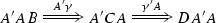
With this perspective in mind, we can rephrase in coalgebraic terms several notions and results developed for coinduction up-to in a lattice-theoretic setting [41]. In particular, up-to techniques can be thought of as functors $A:\mathcal {C}\rightarrow \mathcal {C}$, and B-invariants up to A as BA-coalgebras. For such a functor A to be of interest it has to be B-sound, meaning that it can safely be used to prove the coinductive predicate defined by B. Formally, we say that A is B-sound if there exists a functor $G :\mathsf {Coalg}(BA) \rightarrow \mathsf {Coalg}(B)$ and a natural transformation $\kappa :U\Rightarrow UG$.

(4)

When $\mathcal {C}$ is a partial order, the soundness of A entails that for every B-invariant up-to A, there exists a greater B-invariant. Combined with the coinduction principle (1), this leads to the enhanced principle of coinduction up-to.

It is somehow inconvenient to prove soundness directly since, as we discussed in the Introduction, soundness is not preserved by composition. To avoid this problem, we restrict to those up-to techniques A that are B-compatible, i.e., such that there exists a natural transformation $\gamma :AB \Rightarrow BA$. The most important properties of B-compatible functors, which we show next, are that (a) they are sound (Theorem 3.1), and (b) they are closed under composition and various other operations (Proposition 3.3). The following result generalises [41, Theorem 6.3.9] from lattices to categories.

Theorem 3.1

Let A, B be endofunctors on a category $\mathcal {C}$ with countable coproducts. If A is B-compatible then it is B-sound.

Proof

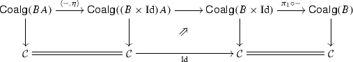
Following the proof of [4, Theorem 3.8], for any BA-coalgebra $\xi$ one can inductively define a family of coalgebras $(\xi _i :A^i X \rightarrow BA^{i+1}X)_{i<\omega }$ by setting $\xi _0 = \xi$ and $\xi _{i+1} = \gamma _{A^{i+1} X} \circ A \xi _i$. Postcomposing with the coproduct injections $\kappa _i :A^i X \rightarrow A^\omega X$ into the coproduct $A^\omega X = \coprod _{i < \omega }A^i X$ yields a cocone $(B\kappa _{i+1} \circ \xi _i :A^i X \rightarrow BA^\omega X)_{i<\omega }$ and hence we obtain from the universal property of the coproduct $A^\omega X$ a B-coalgebra $\xi ^\dagger$ making the next diagram commute.

The mapping $\xi \mapsto \xi ^\dagger$ extends to a functor between the corresponding categories of coalgebras, making the square in the following diagram commute.

We obtain a natural transformation as in (4) using the naturality of $\kappa _0$.

Alternatively, we can replace the countable coproduct $A^\omega$ by the free monad on A, assuming the latter exists. In this case, the result is an instance of the generalised powerset construction [47]. $\square$

To exploit the compositional aspect of compatible up-to techniques to its full potential, it is useful to extend the notion of compatibility to arbitrary functors of type $\mathcal {C}\rightarrow \mathcal {C}'$ rather than just endofunctors.

Definition 3.2

Consider two endofunctors $B:\mathcal {C}\rightarrow \mathcal {C}$ and $B':\mathcal {C}'\rightarrow \mathcal {C}'$. We say that a functor $A:\mathcal {C}\rightarrow \mathcal {C}'$ is $(B,B')$ -compatible when there exists a natural transformation $\gamma :AB\Rightarrow B'A$.

The pair $(A,\gamma )$ is a morphism between endofunctors B and $B'$ in the sense of [32]. Since the examples dealt with in this paper only involve categories which are posets, in these examples we only have one choice of natural transformation $\gamma$, so we omit it from the notation. Moreover, given an endofunctor $B:\mathcal {C}\rightarrow \mathcal {C}$, we will simply write that $A:\mathcal {C}^n\rightarrow \mathcal {C}^m$ is B-compatible, when A is $(B^n,B^m)$-compatible.

The following Proposition generalises the compositionality results for compatible functions on lattices, see [40] or [41, Proposition 6.3.11].

Proposition 3.3

Compatible functors are closed under the following constructions:

• (i) composition: if A is (B, C)-compatible and $A'$ is (C, D)-compatible, then $A'\circ A$ is (B, D)-compatible;

• (ii) pairing: if $(A_i)_{i\in \iota }$ are (B, C)-compatible, then $\langle A_i\rangle _{i\in \iota }$ is $(B,C^\iota )$-compatible;

• (iii) product: if A is (B, C)-compatible and $A'$ is $(B',C')$-compatible, then $A\times A'$ is $(B{\times }B',C{\times }C')$-compatible;

Moreover, for an endofunctor $B :\mathcal {C}\rightarrow \mathcal {C}$,

• (vi) the identity functor $\mathrm {Id}:\mathcal {C}\rightarrow \mathcal {C}$ is B-compatible;

• (v) the constant functor to the carrier of any B-coalgebra is B-compatible, in particular the final one if it exists;

• (vi) the coproduct functor $\coprod :\mathcal {C}^\iota \rightarrow \mathcal {C}$ is $(B^\iota ,B)$-compatible.

Proof

• (i) Given $\gamma :AB\Rightarrow CA$ and $\gamma ':A'C\Rightarrow DA'$ we obtain

  

• (ii) Given natural transformations $\gamma _i:A_iB\Rightarrow CA_i$ for all $i\in \iota$ we obtain a natural transformation

  

• (iii) Given $\gamma :AB\Rightarrow CA$ and $\gamma ' :A'B'\Rightarrow C'A'$ we construct the natural transformation $\gamma \times \gamma ':(A\times A')(B\times B')\Rightarrow (C\times C')(A\times A')$.

Items (vi), (v) and (vi) are trivial. For example, the latter is immediate using the universal property of the coproduct. $\square$

Proposition 3.3 plays a key role in our strategy to prove the soundness of up-to techniques. For instance, to prove B-soundness of the equivalence closure $Eqv :\mathsf {Rel}_X \rightarrow \mathsf {Rel}_X$ (Sect. 2.1), we will first decompose it as $Eqv \triangleq Trn \circ Sym \circ Rfl$, where $Trn , Sym , Rfl :\mathsf {Rel}_X \rightarrow \mathsf {Rel}_X$ are, respectively, functors that map a relation to the transitive, symmetric and reflexive closure. In Sect. 6.2, we will show the B-compatibility of $Trn$, $Sym$ and $Rfl$ (based, in fact, on a further decomposition of $Sym$ and $Rfl$). Then B-compatibility of $Eqv$ follows by Proposition 3.3. Soundness will be a consequence of Theorem 3.1.

3.1 Respectful functors

There exist up-to techniques which are not B-compatible, but are nevertheless B-sound. We will see such an example in Sect. 8.2. In this case, the up-to technique at issue is B-respectful [45], i.e., $B\times \mathrm {Id}$-compatible. A similar problem arises for CCS and more generally, as explained in Sect. 7, it may happen for any GSOS specification. Being B-respectful is a weaker property than B-compatibility that still implies soundness.

Proposition 3.4

Let $A, B :\mathcal {C}\rightarrow \mathcal {C}$ be functors.

• (i) If A is B-compatible then it is $B \times \mathrm {Id}$-compatible.

• (ii) If A is $B \times \mathrm {Id}$-sound and there is a natural transformation $\eta :\mathrm {Id}\Rightarrow A$ then A is B-sound.

• (iii) If A is $B \times \mathrm {Id}$-compatible, then A is B-sound.

Proof

• (i) Given a natural transformation $\gamma :A B \Rightarrow BA$, we have a natural transformation $\langle \gamma \circ A\pi _1, A\pi _2 \rangle :A (B \times \mathrm {Id}) \Rightarrow (B \times \mathrm {Id}) A$.

• (ii) Consider the following diagram.

  

  The existence of the middle square is the $B \times \mathrm {Id}$-soundness of A. The left and right squares are equalities. The above diagram asserts that A is B-sound.

• (iii) Since A is $B\times \mathrm {Id}$-compatible, by Proposition 3.3 the functor $A + \mathrm {Id}$ is also $B \times \mathrm {Id}$-compatible. Hence, by Theorem 3.1, $A+\mathrm {Id}$ is $B \times \mathrm {Id}$-sound. By item (ii), choosing $\eta$ to be the coproduct injection $\kappa _0 :\mathrm {Id}\Rightarrow A + \mathrm {Id}$, we obtain that $A+ \mathrm {Id}$ is B-sound. Using the other coproduct injection $\kappa _1 :A \Rightarrow A + \mathrm {Id}$, this implies that A is B-sound:

  

  where the left square is an equality and the right square comes from the B-soundness of $A+\mathrm {Id}$.$\square$

4 Poset fibrations

Here, we give the basic definitions about fibrations, with the fibration of relations over sets as a running example. We refer the reader to [26] for a more thorough introduction.

An essential example used throughout this paper is that of the fibration of relations over sets $p:\mathsf {Rel}\rightarrow \mathsf {Set}$. The category $\mathsf {Rel}$ has as objects pairs (R, X) where $R\subseteq X^2$ is a relation on X. The morphisms in $\mathsf {Rel}$ are relation preserving maps, that is, a morphism $f:(R,X)\rightarrow (S,Y)$ is a function $f:X\rightarrow Y$ between the underlying sets, such that $(x,y)\in R$ implies $(f(x),f(y))\in Y$. The functor p maps a relation $R\subseteq X^2$ to its underlying set X. Given a set X we denote by $\mathsf {Rel}_X$ the subcategory of $\mathsf {Rel}$ that has as objects pairs (R, X) and whose morphisms are inclusions: they have as underlying arrow the identity on X. That is, $\mathsf {Rel}_X$ is the poset of relations on X ordered by inclusion and seen as a category.

For every function $f:X\rightarrow Y$ in $\mathsf {Set}$ and every relation $S\subseteq Y^2$ we can obtain a relation on X denoted $f^*(S)$ as the inverse image of S: $(x,y)\in f^*(S)$ if and only if $(f(x),f(y))\in S$.

The relation $f^*(S)$ has a universal property: it is the largest among all the relations R on X such that the function f defines a $\mathsf {Rel}$ morphism $f:(X,R)\rightarrow (Y, S)$, i.e., such that $(x,y) \in R$ implies $(f(x),f(y)) \in S$.

The formal definition of a fibration is rather technical, but it essentially captures the idea of having a category of “properties” indexed over a base category. Moreover, for each morphism f in the base category we have a functor $f^*$ satisfying a universal property generalising the one we mentioned above in the special case of relations.

Definition 4.1

Given a functor $p:\mathcal {E}\rightarrow \mathcal {B}$ and an object X of $\mathcal {B}$, the fibre above X is the subcategory $\mathcal {E}_X$ of $\mathcal {E}$ whose objects are mapped by p to X and whose arrows are mapped by p to the identity on X.

Definition 4.2

A functor $p:\mathcal {E}\rightarrow \mathcal {B}$ is called a poset fibration when

• 1. For every object X in $\mathcal {B}$, the fibre $\mathcal {E}_X$ is a poset.

• 2. For every morphism $f:X\rightarrow Y$ in $\mathcal {B}$ and every R in $\mathcal {E}$ with $p(R)=Y$ there exists an object $f^*(R)$ above X (i.e., in $\mathcal {E}_X$) and a map $\widetilde{f_R}:f^*(R)\rightarrow R$ such that every $u:Q\rightarrow R$ in $\mathcal {E}$ sitting above f (i.e., $pu=f$) factors through $\widetilde{f_R}$: there exists a unique map $v:Q\rightarrow f^*(R)$ in $\mathcal {E}_X$ such that $u=\widetilde{f_R}v$.

A map $\widetilde{f_R}$ as above is called a (weak) Cartesian lifting of f and is unique up to isomorphism. If we make a choice of Cartesian liftings, the association $R\mapsto f^*(R)$ gives rise to the so-called reindexing functor $f^*:\mathcal {E}_Y\rightarrow \mathcal {E}_X$. We have that $(\mathrm {id}_X)^*= \mathrm {id}_{\mathcal {E}_X}$, and, since Cartesian liftings are closed under composition, we have $(f\circ g)^*= g^*\circ f^*$.

Remark 4.3

All our proofs work just as fine in the more general setting of arbitrary fibrations, but we considered that the definition of poset fibrations is easier to grasp. For this reason we do not explicitly mention hereafter that the fibrations are posetal, but the reader can safely assume this and skip the rest of the remark. The general definition, see [26], does not require $\mathcal {E}_X$ be a poset, but the maps $\widetilde{f_R}:f^*(R)\rightarrow R$ satisfy a slightly stronger universal property: for any maps $g:Z\rightarrow X$ in $\mathcal {B}$ and for any u sitting above fg, there exists a unique v such that $u=\widetilde{f_R}v$ and $p(v)=g$. Such a map $\widetilde{f_R}$ is called a Cartesian lifting (as opposed to weak Cartesian lifting), and, in general, we have an isomorphism $(f\circ g)^*\cong g^*\circ f^*$ rather than an equality (as is the case in poset fibrations).

Definition 4.4

A functor $p:\mathcal {E}\rightarrow \mathcal {B}$ is called a bifibration if both $p:\mathcal {E}\rightarrow \mathcal {B}$ and $p^ op :\mathcal {E}^ op \rightarrow \mathcal {B}^ op$ are fibrations.

A fibration $p:\mathcal {E}\rightarrow \mathcal {B}$ is a bifibration if and only if each reindexing functor $f^*:\mathcal {E}_Y\rightarrow \mathcal {E}_X$ has a left adjoint $\coprod _f\dashv f^*$, see [26, Lemma 9.1.2].

Example 4.5

The fibration $p:\mathsf {Rel}\rightarrow \mathsf {Set}$ considered in the beginning of this section is a bifibration with the left adjoints $\coprod _f$ given by direct images.

Notice that for any relation R on X, the relation $\coprod _f(R)$ has a similar universal property to the reindexing, namely it is the smallest among all the relations S on Y such that $f:X\rightarrow Y$ maps elements related by R to elements related by S.

Example 4.6

A second example of a bifibration is that of predicates over sets. Let $\mathsf {Pred}$ be the category of predicates whose objects are pairs of sets (P, X) with $P\subseteq X$ and morphisms $f:(P,X)\rightarrow (Q,Y)$ are arrows $f:X\rightarrow Y$ that can be restricted to ${ \left. f \phantom {\big |} \right| _{P} }:P\rightarrow Q$.

The functor mapping predicates to their underlying sets is a bifibration. The fibre $\mathsf {Pred}_X$ sitting above X is the poset of subsets of X ordered by inclusion. The reindexing functors are given by inverse images and their left adjoints by direct images.

Given fibrations $p:\mathcal {E}\rightarrow \mathcal {B}$ and $p':\mathcal {E}'\rightarrow \mathcal {B}$ and $F:\mathcal {B}\rightarrow \mathcal {B}$, we call $\overline{F}:\mathcal {E}\rightarrow \mathcal {E}'$ a lifting of F when $p'\overline{F}=Fp$.

Notice that a lifting $\overline{F}$ restricts to a functor between the fibres $\overline{F}_X:\mathcal {E}_X\rightarrow \mathcal {E}'_{FX}$. When the subscript X is clear from the context we will omit it.

A fibration map from $p:\mathcal {E}\rightarrow \mathcal {B}$ to $p':\mathcal {E}'\rightarrow \mathcal {B}$ is a pair $(\overline{F},F)$ such that $\overline{F}$ is a lifting of F that preserves Cartesian liftings, i.e., for any $\mathcal {B}$-morphism f and Cartesian lifting $\widetilde{f}$ the map $\overline{F}\widetilde{f_R}:\overline{F}f^*(R)\rightarrow \overline{F}R$ is a Cartesian lifting of Ff. This entails that $(Ff)^*\overline{F}\cong \overline{F}f^*$ for any $\mathcal {B}$-morphism f (in fact, in a poset fibration, this isomorphism is an equality). We denote by $\mathsf {Fib}(\mathcal {B})$ the category of fibrations with base $\mathcal {B}$.

Every $\mathsf {Set}$ endofunctor F has a canonical lifting in the fibration $\mathsf {Rel}\rightarrow \mathsf {Set}$, which we call the canonical relation lifting of F and denote by $\mathsf {Rel}(F):\mathsf {Rel}\rightarrow \mathsf {Rel}$. In order to define it, represent $R\in \mathsf {Rel}_X$ as a jointly mono span $X\xleftarrow {\pi _1} R\xrightarrow {\pi _2} X$ and apply F. Then $\mathsf {Rel}(F)(R)$ is obtained as the image of the induced map $FR\rightarrow FX\times FX$. Below, we list a number of important properties of the canonical relation lifting. We use ${\varDelta }_X$ to denote the diagonal relation on X, $R^{-1}$ to denote the converse relation of R and $R \otimes S =\{(x,z) \mid \exists y.~x \mathrel R y \wedge y\mathrel R z\}$ for the composition of relations R and S.

Lemma 4.7

The canonical relation lifting of any $F,G :\mathsf {Set}\rightarrow \mathsf {Set}$ satisfies:

• 1. $\mathsf {Rel}(\mathrm {Id})=\mathrm {Id}$

• 2. $\mathsf {Rel}(F)({\varDelta }_X) = {\varDelta }_{FX}$

• 3. $\mathsf {Rel}(F)(R^{{-1}}) = (\mathsf {Rel}(F)(R))^{{-1}}$

• 4. $\mathsf {Rel}(F)(R \otimes S) \subseteq \mathsf {Rel}(F)(R) \otimes \mathsf {Rel}(F)(S)$

• 5. $\mathsf {Rel}(F)(f^*(R)) \subseteq (Ff)^*\mathsf {Rel}(F)(R)$

• 6. $\mathsf {Rel}(F)(\mathsf {Gr}(f))\subseteq \mathsf {Gr}(Ff)$ where $\mathsf {Gr}(f)$ denotes the graph of a $\mathsf {Set}$-function f.

• 7. $\mathsf {Rel}(FG) = \mathsf {Rel}(F)\mathsf {Rel}(G)$

• 8. $\mathsf {Rel}(F \times G) \cong \mathsf {Rel}(F) \times \mathsf {Rel}(G)$

• 9. Any $\lambda :F \Rightarrow G$ restricts to a natural transformation $\overline{\lambda } :\mathsf {Rel}(F) \Rightarrow \mathsf {Rel}(G)$.

If $F :\mathsf {Set}\rightarrow \mathsf {Set}$ preserves weak pullbacks, then:

• 8. $(\mathsf {Rel}(F),F)$ is a fibration map (i.e., Item 5 above is an equality).

• 9. Item 4 is an equality.

Proof

For 1, 2, 3, 4 and 7, 8, 9 see [27, Propositions 4.4.2, 4.4.3; Exercise 4.4.6]. Items 6, 7 and 8 are standard, but we prove 7 in Lemma 14.1 in “Appendix 1”. $\square$

For a fibration $p :\mathcal {E}\rightarrow \mathcal {B}$ we say that p has fibred finite (co)products if each fibre has finite (co)products, preserved by reindexing functors. If p is a bifibration with fibred finite products and coproducts, and $\mathcal {B}$ has finite products and coproducts, then the total category $\mathcal {E}$ also has finite products and coproducts, strictly preserved by p [26, Propositions 9.1.1 and 9.2.2, Example 9.2.5]. In this paper, we assume the bifibration under consideration to have fibred (co)products only in Sect. 7.

5 Coinductive predicates

In Sect. 3 we have argued that systems are modeled as coalgebras in a certain “base” category, whereas coinductive predicates and invariants are coalgebras in categories of “properties”. As explained in [22, 23], the basic infrastructure for modeling systems and their coinductive properties is provided in a systematic manner by fibrations, as we recall next. Given a fibration $p :\mathcal {E}\rightarrow \mathcal {B}$, the idea is that the systems of interest are modeled as coalgebras for a functor $F :\mathcal {B}\rightarrow \mathcal {B}$. Coinductive predicates for a coalgebra $\xi :X \rightarrow FX$ are then coalgebras themselves, for a functor on the fibre $\mathcal {E}_X$ above X. The key idea is to define such a functor uniformly for each coalgebra by taking a lifting $\overline{F} :\mathcal {E}\rightarrow \mathcal {E}$ of F. Then, given a coalgebra $\xi :X \rightarrow FX$ we define the functor

(5)

The $\overline{F}_{\xi }$-coalgebras are then the invariants of interest, and the final $\overline{F}_{\xi }$-coalgebra, if it exists, is the coinductive predicate defined on $\xi$ by the lifting $\overline{F}$.

Example 5.1

Consider the $\mathsf {Set}$ functor $FX = 2 \times X^A$ of deterministic automata. In Sect. 2 we have defined a monotone function B whose invariants (post-fixed points) are bisimulations on a given deterministic automaton $\xi$, and whose greatest fixed point is language equivalence. This B arises as an instance of (5), by taking the fibration to be the relation fibration $p :\mathsf {Rel}\rightarrow \mathsf {Set}$, and the lifting $\overline{F}$ to be the canonical relation lifting $\mathsf {Rel}(F)$ of F. In this case,

$$\begin{aligned} \mathsf {Rel}(F)(R \subseteq X \times X) = \{((p,\varphi ),(q,\psi )) \mid p = q \text { and } \forall a \in A. \, \varphi (a) \mathrel {R} \psi (a)\}. \end{aligned}$$

It is easy to compute that $\mathsf {Rel}(F)_{\xi }(R) = B(R)$. Hence, $\mathsf {Rel}(F)_{\xi }$-coalgebras are bisimulations on deterministic automata.

In fact, given an arbitrary $\mathsf {Set}$ endofunctor F and a coalgebra $\xi :X \rightarrow FX$, $\mathsf {Rel}(F)_{\xi }$-coalgebras are Hermida–Jacobs bisimulations [23]. But instantiating $\overline{F}$ to a different lifting than the canonical one gives rise to different coinductive predicates.

Example 5.2

Consider the lifting of the functor $FX = 2 \times X^A$ in the relation fibration $p :\mathsf {Rel}\rightarrow \mathsf {Set}$, defined by

$$\begin{aligned} \overline{F}(R \subseteq X \times X) = \{((p,\varphi ),(q,\psi )) \mid p \le q \text { and } \forall a \in A. \, \varphi (a) \mathrel {R} \psi (a)\}. \end{aligned}$$

Then given a deterministic automaton $\xi :X \rightarrow FX$, the functor $\overline{F}_{\xi }$ coincides with the functor $B'$ defined in Sect. 2.3. So, $\overline{F}_{\xi }$-coalgebras are simulations on deterministic automata.

As explained above, a lifting $\overline{F}$ of F defines a functor on the fibre above any F-coalgebra. The following result emphasises that these functors are defined uniformly.

Proposition 5.3

Suppose $(\overline{F},F)$ is a fibration map on a given fibration $p :\mathcal {E}\rightarrow \mathcal {B}$. If $f :X \rightarrow Y$ is a coalgebra homomorphism from $\xi :X \rightarrow FX$ to $\zeta :Y \rightarrow FY$ then there is an adjunction

which lifts the adjunction $\textstyle {\coprod }_f \dashv f^*$.

Proof

Using that $Ff \circ \xi = \zeta \circ f$ (since f is a homomorphism) and that $\overline{F}_X \circ f^* \cong (Ff)^* \circ \overline{F}_Y$ (since $(\overline{F},F)$ is a fibration map) we have the following isomorphism:

$$\begin{aligned} \overline{F}_{\xi } f^* = \xi ^* \overline{F}_X f^* \cong \xi ^* (Ff)^* \overline{F}_Y \cong (Ff \circ \xi )^* \overline{F}_Y = (\zeta \circ f)^* \overline{F}_Y \cong f^* \zeta ^* \overline{F}_Y = f^* \overline{F}_{\zeta }. \end{aligned}$$

The statement of the Lemma now follows from [23, Corollary 2.15]. $\square$

The right adjoint maps the final $\overline{F}_{\zeta }$-coalgebra, i.e., the coinductive predicate defined on $\zeta$ by $\overline{F}$, to the final $\overline{F}_{\xi }$-coalgebra, i.e., the coinductive predicate defined on $\xi$ (which is [22, Proposition 3.11 (ii)]). This captures formally the idea that coinductive predicates, defined in the above way by a functor lifting, are preserved and reflected by coalgebra homomorphisms, if $\overline{F}$ is a fibration map. For the canonical lifting $\mathsf {Rel}(F)$ this is the case whenever F preserves weak pullbacks, see Lemma 4.7. Since bisimilarity on an F-coalgebra $\xi$ is the final $\mathsf {Rel}(F)_{\xi }$-coalgebra, the above proposition is a generalisation of the well-known fact that coalgebra homomorphisms preserve and reflect bisimilarity [44].

6 Up-to techniques in a fibration

Throughout this section we fix a bifibration $p:\mathcal {E}\rightarrow \mathcal {B}$, an endofunctor $F :\mathcal {B}\rightarrow \mathcal {B}$, a lifting $\overline{F}:\mathcal {E}\rightarrow \mathcal {E}$ of F and a coalgebra $\xi :X \rightarrow FX$. As explained in Sect. 5, the studied system $\xi$ lives in the base category $\mathcal {B}$. The lifting $\overline{F}$ defines a coinductive predicate on X as the final coalgebra of the functor $\overline{F}_{\xi } = \xi ^*\circ \overline{F}_X:\mathcal {E}_X \rightarrow \mathcal {E}_X$, and the associated coinductive proof technique amounts to the construction of suitable $\overline{F}_{\xi }$-invariants, i.e., $\overline{F}_{\xi }$-coalgebras.

We instantiate the theory of up-to techniques and compatible functors from the previous section to the category $\mathcal {E}_X$ and the functor $\overline{F}_{\xi }$. In this context, a (potential) up-to technique is a functor $A :\mathcal {E}_X \rightarrow \mathcal {E}_X$. If such a functor A is sound then the construction of $\overline{F}_{\xi }$-invariants up to A is a valid proof technique for the coinductive predicate defined by $\overline{F}_{\xi }$. In this section we introduce three families of up-to techniques A. For each family we provide abstract conditions on the lifting $\overline{F}$ and on A that guarantee their compatibility, and hence their soundness. More specifically, we consider up-to techniques based on behavioural equivalence (Sect. 6.1), transitive and equivalence closure (Sect. 6.2) and contextual closure (Sect. 6.3).

6.1 Compatibility of behavioural equivalence closure

In Sect. 2.2, we have seen that, in coinductive proofs of language equivalence, one can exploit language equivalence itself by using the up-to technique $Bhv$. In [34], Milner introduced up to bisimilarity [34] motivated by a similar intent. From a coalgebraic perspective these two techniques are essentialy the same: both language equivalence and bisimilarity are instances of behavioural equivalence $\sim$, i.e., the kernel of the final morphism $[\![ - ]\!]$.

For a coalgebra $\xi :X \rightarrow FX$, the function $Bhv :\mathsf {Rel}_X \rightarrow \mathsf {Rel}_X$ is defined as

$$\begin{aligned} Bhv (R)= \{(x,y)\mid \exists x',y' \text { s.t. } x \sim x' \mathrel R y' \sim y \}. \end{aligned}$$

By unfolding the definition of $\sim$, this is equivalent to

$$\begin{aligned} Bhv (R)&= \{(x,y) \mid \exists x',y'.\, [\![ x ]\!] =[\![ x' ]\!],\, [\![ y ]\!] =[\![ y' ]\!] \text { and } (x',y') \in R\} \\&= [\![ \{([\![ x' ]\!], [\![ y' ]\!]) \mid (x',y') \in R \} ]\!]^{-1} \\&= [\![ [\![ R ]\!] ]\!]^{-1} \end{aligned}$$

which is just direct image followed by reindexing in the fibration $\mathsf {Rel}\rightarrow \mathsf {Set}$, namely, $[\![ [\![ R ]\!] ]\!]^{-1} = [\![ - ]\!]^* \circ \textstyle {\coprod }_{[\![ - ]\!]} (R)$. This observation allows us to generalise the above function $Bhv$ to an arbitrary bifibration $p :\mathcal {E}\rightarrow \mathcal {B}$, a functor $F :\mathcal {B}\rightarrow \mathcal {B}$ with a final coalgebra, and a coalgebra $\xi :X \rightarrow FX$. In this setting behavioural equivalence closure $Bhv :\mathcal {E}_X\rightarrow \mathcal {E}_X$ is defined as

$$\begin{aligned} Bhv = [\![ - ]\!]^*\circ \textstyle {\coprod }_{[\![ - ]\!]}. \end{aligned}$$

For instance, in the predicate fibration $\mathsf {Pred}\rightarrow \mathsf {Set}$, we have

$$\begin{aligned} Bhv (P) = [\![ [\![ P ]\!] ]\!]^{-1} = [\![ \{[\![ x' ]\!] \mid x' \in P \} ]\!]^{-1} = \{x \mid \exists x' \in P. \, [\![ x ]\!] = [\![ x' ]\!]\}. \end{aligned}$$

The compatibility of $Bhv$ is an instance of:

Theorem 6.1

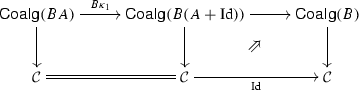
Suppose that $(\overline{F}, F)$ is a fibration map. For any F-coalgebra morphism $f:(X,\xi )\rightarrow (Y,\zeta )$, the functor $f^*\circ \coprod _f$ is $\overline{F}_{\xi }$-compatible.

Proof sketch

We exhibit a natural transformation

$$\begin{aligned} f^*\circ \textstyle {\coprod }_f\circ (\xi ^*\circ \overline{F})\Rightarrow (\xi ^*\circ \overline{F})\circ f^*\circ \textstyle {\coprod }_f \end{aligned}$$

obtained by pasting the 2-cells (a), (b), (c), (d) in the following diagram:

• (a) Since $(\overline{F}, F)$ is a fibration map we have that $\overline{F}f^*\cong (Ff)^*\overline{F}$.

• (b) is a consequence of Lemma 14.3 in “Appendix 2”.

• (c) is a natural isomorphism and comes from the fact that f is a coalgebra map.

• (d) is obtained from (c) using the counit of $\coprod _{f}\dashv f^*$ and the unit of $\coprod _{Ff}\dashv (Ff)^*$.

(Note that this proof decomposes into a proof that $\coprod _f$ is $(\overline{F}_{\xi },\overline{F}_{\zeta })$-compatible, by pasting (b) and (d), and a proof that $f^*$ is $(\overline{F}_{\zeta },\overline{F}_{\xi })$-compatible, by pasting (a) and (c). These two independent results can be composed by Proposition 3.3(i) to obtain the theorem.) $\square$

Corollary 6.2

If F is a $\mathsf {Set}$-functor preserving weak pullbacks then the behavioural equivalence closure functor $Bhv$ is $\mathsf {Rel}(F)_{\xi }$-compatible.

Proof

The result follows from Lemma 4.7 and Theorem 6.1. $\square$

Both the functor $FX=(\mathcal {P}_{\omega }X)^L$ for labeled transition systems and the functor $FX=2\times X^A$ for deterministic automata preserve weak pullbacks. Hence, Corollary 6.2 provides the compatibility of both Milner’s up-to-bisimilarity and $Bhv$ as used in Sect. 2.2.

From Theorem 6.1 we also derive the soundness of up-to $Bhv$ for unary predicates: the monotone predicate liftings used in coalgebraic modal logic [17] are fibration maps [27], so they satisfy the hypothesis of Theorem 6.1.

6.2 Compatibility of equivalence closure

We propose a general approach for deriving the compatibility of the reflexive, symmetric and transitive closure. Composing these functors yields compatibility of the equivalence closure, as outlined in Sect. 3.

For the transitive closure, it suffices to prove that relational composition is compatible. Composition of relations can be expressed in a fibrational setting, by considering the category $\mathsf {Rel}\times _{\mathsf {Set}} \mathsf {Rel}$ obtained as a pullback of the fibration $\mathsf {Rel}\rightarrow \mathsf {Set}$ along itself:

The objects of $\mathsf {Rel}\times _\mathsf {Set}\mathsf {Rel}$ are pairs of relations $R,S \subseteq X \times X$ on a common carrier X. An arrow from $R,S \subseteq X \times X$ to $R',S' \subseteq Y \times Y$ is a pair of morphisms in $\mathsf {Rel}$ above a common $f :X \rightarrow Y$; thus, it is a map $f :X \rightarrow Y$ such that $f(R) \subseteq R'$ and $f(S) \subseteq S'$. Relational composition is a functor $\otimes :\mathsf {Rel}\times _{\mathsf {Set}} \mathsf {Rel}\rightarrow \mathsf {Rel}$ mapping $R,S\subseteq X \times X$ to their composition $R\otimes S$.

The pullback $\mathsf {Rel}\times _\mathsf {Set}\mathsf {Rel}$ above is, in fact, a product in the category $\mathsf {Fib}(\mathsf {Set})$ of fibrations over $\mathsf {Set}$. Indeed, $\mathsf {Rel}\times _\mathsf {Set}\mathsf {Rel}\rightarrow \mathsf {Set}$ is again a fibration. In order to treat not only relational composition but also, e.g., symmetric and reflexive closure, we move to a more general setting of n-fold products. Consider for an arbitrary fibration $\mathcal {E}\rightarrow \mathcal {B}$ its n-fold product in $\mathsf {Fib}(\mathcal {B})$ (see [26, Lemma 1.7.4]), denoted by $\mathcal {E}^{\times _{\mathcal {B}}^n}\rightarrow \mathcal {B}$ and defined by pullback in $\mathsf {Cat}$. This product is computed fibrewise, that is,

$$\begin{aligned} (\mathcal {E}^{\times _{\mathcal {B}}^n})_X = (\mathcal {E}_X)^n \quad \text { and } \quad \mathcal {E}^0 = \mathcal {B}. \end{aligned}$$

Concretely, the objects in $\mathcal {E}^{\times _{\mathcal {B}}^n}$ are n-tuples of objects in $\mathcal {E}$ belonging to the same fibre, and an arrow from $(R_1, \ldots , R_n)$ above X to $(S_1, \ldots , S_n)$ above Y consists of a tuple of arrows $(f_1 :R_1 \rightarrow S_1, \ldots , f_n :R_n \rightarrow S_n)$ that sit above a common $f :X \rightarrow Y$.

It turns out that we can capture composition, relation converse and the functor mapping a set to the diagonal relation as functors of the form $G:\mathcal {E}^{\times _{\mathcal {B}}^n}\rightarrow \mathcal {E}$ that have the additional property to be liftings of the identity functor on $\mathcal {B}$. Given such a functor G, for each X in $\mathcal {B}$ we have a functor $G_X:(\mathcal {E}_X)^n \rightarrow \mathcal {E}_X$.

Proposition 6.3

Let $\overline{F}:\mathcal {E}\rightarrow \mathcal {E}$ be a lifting of a $\mathcal {B}$-functor F and $G:\mathcal {E}^{\times _{\mathcal {B}}n}\rightarrow \mathcal {E}$ be a lifting of the identity, and suppose that for each X in $\mathcal {B}$ there is a natural transformation

$$\begin{aligned} \gamma :G_{FX} \circ (\overline{F}_X)^n \Rightarrow \overline{F}_X \circ G_X : (\mathcal {E}_X)^n \rightarrow \mathcal {E}_{FX}. \end{aligned}$$

Then for any coalgebra $\xi :X \rightarrow FX$, the functor $G_X$ is $\overline{F}_{\xi }$-compatible.

We list several applications of the proposition for the fibration $\mathsf {Rel}\rightarrow \mathsf {Set}$. In this case, a natural transformation $G_{FX} \circ (\overline{F}_X)^n \Rightarrow \overline{F}_X \circ G_X$ exists precisely if for all relations $R_1, \ldots , R_n$ on the carrier X:

$$\begin{aligned} G (\overline{F}(R_1), \ldots , \overline{F}(R_n)) \subseteq \overline{F} G(R_1, \ldots , R_n). \end{aligned}$$

Instantiating this, we obtain as a corollary of Proposition 6.3 concrete compatibility results for functors $\mathsf {Rel}^{\times _\mathsf {Set}^n} \rightarrow \mathsf {Rel}$, including relational composition.

Lemma 6.4

The following hold:

$(n{=}0)$ :

Let $Dia :\mathsf {Set}\rightarrow \mathsf {Rel}$ be the functor mapping each set X to ${\varDelta }_X$, the diagonal relation on X. $Dia _X :1 \rightarrow \mathsf {Rel}_X$ is $\overline{F}_{\xi }$-compatible if

$(n{=}1)$ :

Let $Inv :\mathsf {Rel}\rightarrow \mathsf {Rel}$ be the functor mapping each relation $R\subseteq X^2$ to its converse $R^{-1}\subseteq X^2$. $Inv _X :\mathsf {Rel}_X \rightarrow \mathsf {Rel}_X$ is $\overline{F}_{\xi }$-compatible if for all relations $R\subseteq X^2$

$(n{=}2)$ :

Let $\otimes :\mathsf {Rel}\times _\mathsf {Set}\mathsf {Rel}\rightarrow \mathsf {Rel}$ be the relational composition functor. Then $\otimes _X :\mathsf {Rel}_X \times \mathsf {Rel}_X \rightarrow \mathsf {Rel}_X$ is $\overline{F}_{\xi }$-compatible if for all $R,S\subseteq X^2$

If moreover $T_1,T_2:\mathsf {Rel}_X\rightarrow \mathsf {Rel}_X$ are two $\overline{F}_{\xi }$-compatible functors, their pointwise composition $T_1\otimes T_2=\otimes _X\circ \langle T_1,T_2\rangle$ is $\overline{F}_{\xi }$-compatible by Proposition 3.3 (i,ii).

Consider the reflexive closure functor $Rfl _X$, defined by:

If (*) holds in the above Lemma, then $Dia _X$ is compatible, hence $Rfl _X$ is compatible by Proposition 3.3.

Similarly, the symmetric closure functor $Sym _X :\mathsf {Rel}_X \rightarrow \mathsf {Rel}_X$ is the coproduct of $\mathrm {Id}$ and $Inv _X$, i.e.,

$$\begin{aligned} Sym _X=\coprod \circ \langle \mathrm {Id}, Inv _X\rangle . \end{aligned}$$

Hence by Proposition 3.3, $Sym _X$ is $\overline{F}_{\xi }$-compatible whenever $(*{*})$ holds.

Corollary 6.5

Given a $\mathsf {Set}$-functor F and a relation lifting $\overline{F}$ such that $(*{*}*)$ holds, then the transitive closure functor $Trn _X$ is $\overline{F}_{\xi }$-compatible.

Proof

The transitive closure functor $Trn _X$ is obtained from $\otimes$ in a modular way:

$$\begin{aligned} Trn _X=\coprod _{i\ge 0} (-)^i:\mathsf {Rel}_X\rightarrow \mathsf {Rel}_X \end{aligned}$$

where $(-)^0=\mathrm {Id}$ and $(-)^{i+1}=\mathrm {Id}\otimes (-)^i$. Using item (vi) of Proposition 3.3, it suffices to show that each $(-)^i$ is $\overline{F}_{\xi }$-compatible. This in turn can be proved by induction using item (vi) of Proposition 3.3 and the third part of Lemma 6.4. $\square$

By Proposition 3.3, given the compatibility of $Rfl _X$, $Sym _X$ and $\otimes _X$ (and hence of $Trn _X$), one obtains compatibility of the equivalence closure functor $Eqv _X$, defined by

$$\begin{aligned} Eqv _X = Trn _X \circ Sym _X \circ Rfl _X\,. \end{aligned}$$

From the above considerations we get the following result for the canonical relation lifting of a $\mathsf {Set}$ functor.

Corollary 6.6

If F is a $\mathsf {Set}$-functor then the reflexive and symmetric closure functors $Rfl _X$ and $Sym _X$ are $\mathsf {Rel}(F)_{\xi }$-compatible. Moreover, if F preserves weak pullbacks, then the transitive closure functor $Trn _X$ and the equivalence closure functor $Eqv _X$ are both $\mathsf {Rel}(F)_{\xi }$-compatible.

Proof

By Lemma 4.7, the conditions $(*)$ and $(**)$ from Lemma 6.4 always hold for the canonical lifting $\overline{F}=\mathsf {Rel}(F)$, and $(*{*}*)$ holds when F preserves weak pullbacks. As a consequence of Lemma 6.4 and Corollary 6.5, the functors $Rfl _X$, $Sym _X$ and $Trn _X$ are $\mathsf {Rel}(F)_{\xi }$-compatible. Compatibility of $Eqv _X$ follows since it is a composition of compatible functors, as explained above. $\square$

In particular, the fact that $Eqv _X$ is B-compatible, for the endofunctor B defined in Sect. 2.1, follows from Corollary 6.6 and the characterisation of B given in Example 5.1.

When $\overline{F}_{\xi }$ has a final coalgebra ${\varOmega }$, one can define a “self closure” $\mathcal {E}_X$-endofunctor $Slf =\widetilde{{\varOmega }}\otimes \mathrm {Id}\otimes \widetilde{{\varOmega }}$, where $\widetilde{{\varOmega }}:\mathcal {E}_X\rightarrow \mathcal {E}_X$ is the constant to ${\varOmega }$ functor. Thanks to Proposition 3.3, the functor $Slf$ is $\overline{F}_{\xi }$-compatible whenever $(*{*}*)$ holds. For instance, one can prove compatibility of $Slf$ for the endofuctor $B'$ of Sect. 2.3 by checking that $(*{*}*)$ holds for $\overline{F}$ defined as in Example 5.2.

If $\overline{F}$ is instantiated to the canonical lifting $\mathsf {Rel}(F)$, then ${\varOmega }$ is the bisimilarity relation. In this case, if F preserves weak pullbacks, then ${\varOmega }$ coincides with behavioural equivalence, so then $Slf = Bhv$.

If instead we consider the lifting that yields weak bisimilarity (to be defined in Sect. 9), $Slf$ corresponds to a technique called “weak bisimulation up to weak bisimilarity”, while $Bhv$ corresponds to “weak bisimulation up to (strong) bisimilarity”.

6.3 Compatibility of contextual closure

Up-to context is a technique of pivotal importance for coinductive proofs of systems specified by some syntax, such as process calculi or regular expressions. In these cases, we are in the presence of a coalgebra $\xi :X\rightarrow FX$ equipped with an algebraic structure $\alpha :TX \rightarrow X$, for some functors $F,T :\mathsf {Set}\rightarrow \mathsf {Set}$. The contextual closure $Ctx :\mathsf {Rel}_X \rightarrow \mathsf {Rel}_X$ is defined for all relations $R\subseteq X^2$ as

$$\begin{aligned} Ctx (R)= (\alpha \times \alpha )(\mathsf {Rel}(T)(R)). \end{aligned}$$

When T is the free monad generated by some signature S (i.e., the term monad mapping each set X to the set of S-terms with variables in X) and the algebra is the initial T-algebra $\mu _0:TT0 \rightarrow T0$, $Ctx (R)$ is simply the relation defined by the rules

where f is an arbitrary operator of S of arity n and $s,s_i,t,t_i$ are terms in T0. It is easy to see that this definition generalises the contextual closure introduced for regular expressions in Sect. 2.2.

The notion of contextual closure can be further generalised for an arbitrary bifibration $p:\mathcal {E}\rightarrow \mathcal {B}$, a lifting $\overline{T}$ of the functor $T:\mathcal {B}\rightarrow \mathcal {B}$ and an algebra $\alpha :TX \rightarrow X$ as follows:

(6)

To prove compatibility of this technique, it is essential to require that the algebraic structure $\alpha$ “behaves well” with respect to the coalgebra $\xi$. For this reason, we assume that $(X, \alpha , \xi )$ is a $\rho$ -bialgebra for a distributive law¹ $\rho :TF\Rightarrow FT$, which means that the following diagram commutes:

(7)

Our compatibility theorem requires that $\rho$ lifts to the total category $\mathcal {E}$.

Theorem 6.7

Let $\overline{T},\overline{F}:\mathcal {E}\rightarrow \mathcal {E}$ be liftings of T and F. If $\overline{\rho } :\overline{T}\,\overline{F}\Rightarrow \overline{F}\,\overline{T}$ is a natural transformation sitting above $\rho$, then $\coprod _\alpha \circ \,\overline{T}$ is $\overline{F}_{\xi }$-compatible.

Proof sketch

We exhibit a natural transformation

$$\begin{aligned} (\textstyle {\coprod }_\alpha \circ \overline{T})\circ (\xi ^*\circ \overline{F}) \Rightarrow (\xi ^*\circ \overline{F})\circ (\textstyle {\coprod }_\alpha \circ \overline{T}). \end{aligned}$$

This is achieved in Fig. 1 by pasting five natural transformations, obtained as follows:

• (a) is the counit of the adjunction $\coprod _{\rho _X}\dashv \rho _X^*$.

• (b) comes from $\overline{\rho }$ being a lifting of $\rho$, see Lemma 14.5.

• (c) comes from the bialgebra condition, and the units and counits of the adjunctions $\coprod _{\alpha }\dashv \alpha ^*$, $\coprod _{F\alpha }\dashv (F\alpha )^*$, and $\coprod _{\rho _X}\dashv \rho _X^*$, see Lemma 14.6.

• (d) arises since $\overline{T}$ is a lifting of T, using the universal property of the Cartesian lifting $(T\xi )^*$, see Lemma 14.2.

• (e) comes from $\overline{F}$ being a lifting of F, combined with the unit and counit of the adjunction $\coprod _{\alpha }\dashv \alpha ^*$, see Lemma 14.3.

(As for Theorem 6.1, this proof decomposes into a proof that $\overline{T}$ is $(\overline{F}_{\xi },(T\xi )^*\circ \rho _X^*\circ \overline{F})$-compatible, and a proof that $\coprod _\alpha$ is $((T\xi )^*\circ \rho _X^*\circ \overline{F},\overline{F}_{\xi })$-compatible.) $\square$

Fig. 1

Compatibility of contextual closure in a fibration

When $\overline{F}$ and $\overline{T}$ are the canonical liftings $\mathsf {Rel}(F)$ respectively $\mathsf {Rel}(T)$ in the relation fibration, we get as a corollary the following result, equivalent to Theorem 4 in [43].

Corollary 6.8

If F, T are $\mathsf {Set}$-functors and $(X, \alpha , \xi )$ is a bialgebra for $\rho :T F \Rightarrow F T$, then the contextual closure functor $Ctx$ is $\mathsf {Rel}(F)_{\xi }$-compatible.

Proof

By [27, Exercise 4.4.6], the canonical relation lifting preserves natural transformations, i.e., there is a natural transformation $\overline{\rho } :\mathsf {Rel}(TF) \Rightarrow \mathsf {Rel}(FT)$ above $\rho$. By Lemma 14.1, using that every $\mathsf {Set}$ functor preserves epis, we obtain the desired $\overline{\rho } :\mathsf {Rel}(T)\mathsf {Rel}(F) \Rightarrow \mathsf {Rel}(F)\mathsf {Rel}(T)$. $\square$

Our interest in Theorem 6.7 is not restricted to proving compatibility of up to $Ctx$: taking different liftings $\overline{T}$ yields different types of contextual closure, similar to the fact that taking different liftings $\overline{F}$ yields different coinductive predicates. Indeed, in Sect. 8 we consider the left contextual closure for reasoning about divergence, and the monotone contextual closure for weighted automata; both these variants of the contextual closure (instances of (6)) substantially differ from $Ctx$.

In order to apply Theorem 6.7 in situations where either $\overline{T}$ or $\overline{F}$ is not the canonical relation lifting, one has to exhibit a $\overline{\rho }$ sitting above $\rho$. In $\mathsf {Rel}$, such a $\overline{\rho }$ exists if and only if for all relations $R\subseteq X^2$, the restriction of $\rho _X \times \rho _X$ to $\overline{T}\,\overline{F}R$ corestricts to $\overline{F}\,\overline{T}R$, i.e., $(\rho _X \times \rho _X)(\overline{T}\, \overline{F}(R)) \subseteq \overline{F} \, \overline{T}(R)$, or equivalently, $\coprod _{\rho _X}(\overline{T}\,\overline{F}R)\subseteq \overline{F}\,\overline{T}R$. A similar condition has to be checked in the fibration $\mathsf {Pred}\rightarrow \mathsf {Set}$.

6.4 Summary

We present a short summary of the compatibility results of this section. We assume a bifibration $p :\mathcal {E}\rightarrow \mathcal {B}$, a $\mathcal {B}$-endofunctor F with a lifting $\overline{F}$, and a coalgebra $\xi :X \rightarrow FX$. The definition of $Bhv$ relies on the existence of a final F-coalgebra, where $[\![ - ]\!]$ is the unique morphism to the final coalgebra. For contextual closure we assume a $\mathcal {B}$-endofunctor T with a lifting $\overline{T}$, an algebra $\alpha :TX \rightarrow X$ and a natural transformation $\rho :TF \Rightarrow FT$.

Notation	Definition	Condition $\overline{F}_{\xi }$-compatibility
$Bhv$	$[\![ - ]\!]^* \circ \textstyle {\coprod }_{[\![ - ]\!]}$	$(\overline{F},F)$ is a fibration map
–	$\textstyle {\coprod }_{\alpha } \circ \overline{T}$	$(X,\alpha ,\xi )$ is a $\rho$-bialgebra, and there is a distributive law of $\overline{T}$ over $\overline{F}$ above $\rho$

If p is the relation bifibration $\mathsf {Rel}\rightarrow \mathsf {Set}$, we have the following additional results. For the definition of $Slf$ below, we assume that $\overline{F}_{\xi }$ has a final coalgebra with carrier ${\varOmega }$.

Notation	Definition	Condition $\overline{F}_{\xi }$-compatibility
$Rfl _X$	reflexive closure	${\varDelta }_{FX}\subseteq \overline{F}({\varDelta }_X)$
$Sym _X$	symmetric closure	$(\overline{F}R)^{-1}\subseteq \overline{F}(R^{-1})$ for all $R \subseteq X^2$
$\otimes _X$	rel. composition	$\overline{F}(R) \otimes \overline{F}(S) \subseteq \overline{F}(R\otimes S)$ for all $R,S \subseteq X^2$
$Slf$	$R \mapsto {\varOmega } \otimes R \otimes {\varOmega }$	$\otimes _X$ is $\overline{F}_{\xi }$-compatible
$Trn _X$	transitive closure	$\otimes _X$ is $\overline{F}_{\xi }$-compatible
$Eqv _X$	equivalence closure	$Rfl _X$, $Sym _X$ and $\otimes _X$ are $\overline{F}_{\xi }$-compatible
$Ctx$	$\textstyle {\coprod }_{\alpha } \circ \mathsf {Rel}(T)$	$(X,\alpha ,\xi )$ is a $\rho$-bialgebra

7 Abstract GSOS

We now consider up-to-context techniques to reason about models of abstract GSOS, which provides specification formats for defining operations on coalgebras, and allows us to study operational semantics in a general fashion. An abstract GSOS specification is a natural transformation of the form $\lambda :S(F \times \mathrm {Id}) \Rightarrow FT$, where T is the free monad for S, assumed to exist. The name abstract GSOS is motivated by the fact that, as shown in [29, 54], it generalizes the the standard GSOS specification format [6].

A model of a specification $\lambda$ is a triple $(X,\alpha ,\xi )$, where $\xi :X \rightarrow FX$ is a coalgebra and $\alpha :SX \rightarrow X$ an algebra such that the following diagram commutes:

(8)

where $\alpha ^{\sharp } :TX \rightarrow X$ is the algebra for the free monad T defined as the inductive extension of $\alpha$.

Example 7.1

The concrete GSOS rule format [6] can be retrieved by taking F to be the functor $FX=(\mathcal {P}_{\omega }X)^L$ for labeled transition systems and S to be a polynomial functor representing an algebraic signature. In this case, TX is the set of terms over this signature with variables in X. The notion of model as given in (8) corresponds to the usual notion of model of a GSOS specification. Informally, it means that all and only the transitions of $\xi$ can be derived by instantiating the rules in the specification.

In order to have a concrete grasp, consider the parallel operator of CCS [34], whose semantics is defined by the following GSOS rules:

$$\begin{aligned} \frac{p\mathop {\rightarrow }\limits ^{\mu }p'}{p|q \mathop {\rightarrow }\limits ^{\mu }p'|q} \qquad \frac{q\mathop {\rightarrow }\limits ^{\mu }q'}{p|q \mathop {\rightarrow }\limits ^{\mu }p|q'} \qquad \frac{p\mathop {\rightarrow }\limits ^{a}p'\quad q\mathop {\rightarrow }\limits ^{\overline{a}}q'}{p|q \mathop {\rightarrow }\limits ^{\tau }p'|q'} \end{aligned}$$

where $\mu$ ranges over arbitrary actions, namely inputs $a,b, \dots$ outputs $\overline{a},\overline{b},\dots$ or the internal action $\tau$. Take $SX=X \times X$ (for the binary parallel operator) and $F=(\mathcal {P}_{\omega }-)^L$ where L is the set of all actions. For every set X, the corresponding distributive law $\lambda _X :S(FX \times X) \rightarrow FTX$ maps $(f,x,g,y)\in (\mathcal {P}_{\omega }X)^L\times X \times (\mathcal {P}_{\omega }X)^L\times X$ to the function

$$\begin{aligned} \mu \mapsto {\left\{ \begin{array}{ll} \{(x',y) \mid x'\in f(\mu )\}\cup \{(x,y') \mid y'\in g(\mu ) \} &{} \mu \ne \tau \\ \begin{array}{l} \{(x',y) \mid x'\in f(\tau )\} \cup \{(x,y') \mid y'\in g(\tau ) \}\\ \qquad {} \cup \{(x',y') \mid \exists a. \, x'\in f(a), y'\in g(\overline{a})\} \end{array}&\mu =\tau \end{array}\right. } \end{aligned}$$

(9)

Now take X to be the set of all CCS processes, $\xi :X \rightarrow (\mathcal {P}_{\omega }X)^L$ the LTS generated by the standard semantics of CCS [34] and $\alpha :X\times X \rightarrow X$ to be the algebra mapping a pair of processes (p, q) to their parallel composition p|q. It is easy to see that diagram (8) commutes, i.e., $(X,\alpha , \xi )$ is a model for $\lambda$.

Example 7.2

In Sect. 2.2 we recalled how to turn the set RE of regular expressions into an automaton based on inference rules for each of the operators. These rules induce an abstract GSOS specification where $FX = 2 \times X^A$ and $SX = (X \times X) + (X \times X) + X + A + 1 + 1$ modeling two binary operators $+$ and $\cdot$, a unary operator $*$, constants a for each $a \in A$ and constants 0 and 1. The abstract GSOS specification $\lambda :S((2 \times \mathrm {Id}^A) \times \mathrm {Id}) \Rightarrow 2 \times (T(\mathrm {Id}))^A$ is then defined by cases according to the rules; for instance, the two rules for $*$

define, for each set X, the component $\lambda _X^{(*)} :2 \times X^A \times X \rightarrow 2 \times (TX)^A$ of $\lambda$ given by

$$\begin{aligned} \lambda _X^{(*)}(p,\varphi ,x)&= (1, a \mapsto \varphi (a) \cdot x^*) \end{aligned}$$

for all $p\in 2$, $\varphi \in X^A$ and $x\in X$. The two rules for $\cdot$

define the function $\lambda _X^{(\cdot )} :(2 \times X^A \times X) \times (2 \times X^A \times X) \rightarrow 2 \times (TX)^A$ as

$$\begin{aligned} \lambda _X^{(\cdot )}((p,\varphi ,x), (q,\psi ,y) )&= (p\wedge q, a \mapsto \varphi (a) \cdot y + p \cdot \psi (a)) \end{aligned}$$

for all $p,q\in 2$, $\varphi ,\psi \in X^A$ and $x,y\in X$. Observe that the set of regular expressions RE is just T0 for T the free monad over S. By taking $\alpha :S(RE)\rightarrow RE$ to be the initial S-algebra and $\xi :RE\rightarrow F(RE)$ to be the automaton $\langle o,t\rangle$ defined by the Brzozowki derivatives in Sect. 2.2, it is easy to see that $(RE,\alpha ,\xi )$ is a model for $\lambda$.

An abstract GSOS specification $\lambda$ and a model $(X,\alpha ,\xi )$ for it uniquely correspond to, respectively, a distributive law $\rho _{\lambda } :T(F \times \mathrm {Id}) \Rightarrow (F \times \mathrm {Id})T$ of the monad T over the copointed functor $F \times \mathrm {Id}$ and a bialgebra $(X,\alpha ^{\sharp },\langle \xi ,\mathrm {id}\rangle )$ for $\rho _{\lambda }$. For details, see “Appendix 3” or [29, 54]. Hereafter, to make the notation lighter we will often refer to $\rho _\lambda$ as to $\rho$. This construction entails compatibility of the contextual closure.

Corollary 7.3

Let $\lambda :S(F \times \mathrm {Id}) \Rightarrow FT$ be an abstract GSOS specification and let $(X,\alpha ,\xi )$ a model for it. Then $\textstyle {\coprod }_{\alpha ^\sharp } \circ \mathsf {Rel}(T)$ is $(\mathsf {Rel}(F)\times \mathrm {Id})_{\langle \xi , \mathrm {id}\rangle }$-compatible.

Proof

From Corollary 6.8 we immediately obtain $\mathsf {Rel}(F\times \mathrm {Id})_{\langle \xi , \mathrm {id}\rangle }$-compatibility. To conclude, it is enough to observe that $\mathsf {Rel}(F\times \mathrm {Id}) \cong \mathsf {Rel}(F)\times \mathrm {Id}$ by Lemma 4.7. $\square$

In the case of non-canonical liftings, to prove compatibility of contextual closure for bialgebras of a distributive law $\rho _{\lambda }$ generated from an abstract GSOS specification, one should exhibit a natural transformation $\overline{\rho _{\lambda }}$ above $\rho _{\lambda }$ and then apply Theorem 6.7. We next show how to simplify such a task by proving that, under mild additional conditions, it suffices to show that there exists $\overline{\lambda } :\overline{S} (\overline{F} \times \mathrm {Id}) \Rightarrow \overline{F}\,\overline{T}$ above $\lambda$. Here $\overline{T}$ is the free monad of $\overline{S}$ which, by Lemma 14.7 in “Appendix 3”, is a lifting of T.

Theorem 7.4

Let $(X,\alpha ,\xi )$ and $(X,\alpha ^{\sharp },\langle \xi ,\mathrm {id}\rangle )$ be a model and a bialgebra for, respectively, an abstract GSOS specification $\lambda :S(F \times \mathrm {Id}) \Rightarrow FT$ and the corresponding distributive law $\rho _{\lambda }:T(F\times \mathrm {Id}) \Rightarrow (F\times \mathrm {Id}) T$. Let $\overline{S},\overline{F}$ be liftings of S, F and assume that $\overline{S}$ has a free monad $\overline{T}$.

If there is a natural transformation $\overline{\lambda } :\overline{S}(\overline{F} \times \mathrm {Id})\Rightarrow \overline{F}\overline{T}$ sitting above $\lambda$, then

• 1. there exists $\overline{\rho _{\lambda }} :\overline{T}\,(\overline{F} \times \mathrm {Id})\Rightarrow (\overline{F} \times \mathrm {Id})\overline{T}$ sitting above $\rho _{\lambda }$;

• 2. $\textstyle {\coprod }_{\alpha ^\sharp } \circ {\overline{T}}$ is $(\overline{F}\times \mathrm {Id})_{\langle \xi ,\mathrm {id}\rangle }$-compatible.

It is easy to see that 2 is a direct consequence of 1 and Theorem 6.7. The idea of the proof for 1 is that the distributive law $\overline{\rho _{\lambda }}$ is constructed from $\overline{\lambda }$ in the same way as $\rho _{\lambda }$ is constructed from $\lambda$ (see “Appendix 3” for details). By relating free algebras in $\mathcal {E}$ to free algebras in $\mathcal {B}$, one then shows that $\overline{\rho _{\lambda }}$ sits above $\rho _{\lambda }$.

Observe that both Corollary 7.3 and Theorem 7.4 state compatibility with respect to a functor which is not exactly $\overline{F}_{\xi }$, the functor of our interest. A similar issue was encountered in Sect. 3.1, where we dealt with B-respectful functors, i.e., functors that are $B\times \mathrm {Id}$-compatible. The following lemma allows to link GSOS specifications and respectful functors.

Lemma 7.5

There is a natural isomorphism $(\overline{F}\times \mathrm {Id})_{\langle \xi ,\mathrm {id}\rangle } \cong \overline{F}_{\xi } \times \mathrm {Id}$ where the latter product is taken in the fibre $\mathcal {E}_X$.

Proof

Consider an object R in $\mathcal {E}_X$. The product $\overline{F} R \times R$ in $\mathcal {E}$ is above $FX \times X$, whose projections we denote by $\pi _1 :FX \times X \rightarrow FX$ and $\pi _2 :FX \times X \rightarrow X$. By [26, Proposition 9.2.1], we have $\overline{F}R \times R \cong \pi _1^*(\overline{F}R) \times \pi _2^*(R)$ where the latter product is taken in $\mathcal {E}_{FX \times X}$. Thus:

$$\begin{aligned} (\overline{F}\times \mathrm {Id})_{\langle \xi ,\mathrm {id}\rangle } (R)&= \langle \xi , \mathrm {id}\rangle ^*(\overline{F} R \times R) \\&\cong \langle \xi , \mathrm {id}\rangle ^* (\pi _1^*(\overline{F}R) \times \pi _2^*(R)) \\&\cong (\langle \xi , \mathrm {id}\rangle ^* \pi _1^*(\overline{F}R)) \times (\langle \xi , \mathrm {id}\rangle ^* \pi _2^*(R)) \\&\cong \xi ^* \overline{F} R \times R = (\overline{F}_{\xi } \times \mathrm {Id})(R). \end{aligned}$$

The third step holds since reindexing functors preserve products by assumption. $\square$

Example 7.6

In Example 7.2, we have seen that regular expressions carries a model $(RE,\alpha ,\xi )$ for the GSOS specification corresponding to the Brzozowski derivatives. From Corollary 7.3, we have that $\textstyle {\coprod }_{\alpha ^\sharp } \circ \mathsf {Rel}(T)$ is $(\mathsf {Rel}(F)\times \mathrm {Id})_{\langle \xi , \mathrm {id}\rangle }$-compatible. As explained in Sect. 6.3, $\textstyle {\coprod }_{\alpha ^\sharp } \circ \mathsf {Rel}(T)$ is just $Ctx$ as defined in Sect. 2.2. Moreover, by Lemma 7.5, $Ctx$ is $\mathsf {Rel}(F)_{\xi } \times \mathrm {Id}$-compatible. The technique $Bhv$ used in Sect. 2.2 is B-compatible and thus, by Proposition 3.4(i), it is $B\times \mathrm {Id}$-compatible. By Proposition 3.3(i), $Bhv \circ Ctx$ is $B\times \mathrm {Id}$-compatible. B-soundness follows from Proposition 3.4(iii). We conclude that the composite technique $Bhv \circ Ctx$ used in Sect. 2.2 is $\mathsf {Rel}(F)_{\xi }$-sound, and thus B-sound (see Example 5.1).

Now we could use a similar strategy to prove the compatibility of $Slf \circ Ctx$ with respect to the functor $B'$ for simulation introduced in Sect. 2.3. Since, as shown in Example 5.2, this arises from a non-canonical lifting, we should use Theorem 7.4 rather than Corollary 7.3. However, at the end of this paper (Example 13.4), we will provide a simpler proof which avoids to exhibit the natural transformation $\overline{\lambda }$.

We conclude this section with a technical observation. Theorem 7.4, and similarly Corollary 7.3, provides compatibility for a contextual closure induced by the free monad $\overline{T}$ rather than the lifted functor $\overline{S}$ itself, which may be the one presented in concrete cases. However, as shown by the next lemma, the contextual closure defined by $\overline{S}$ is, in each fibre, below the one defined by $\overline{T}$, so if the latter is sound, the former is sound as well.

Lemma 7.7

Let $S, \overline{S}$, T and $\overline{T}$ be as in Theorem 7.4. Given an algebra $\alpha :S X \rightarrow X$ with induced algebra $\alpha ^\sharp :T X \rightarrow X$ for the free monad T, there exists a natural transformation of the form $\textstyle {\coprod }_{\alpha } \circ \overline{S} \Rightarrow \textstyle {\coprod }_{\alpha ^\sharp } \circ \overline{T}$.

8 Examples

8.1 Inclusion of weighted automata

To illustrate the theory in Sect. 6, we consider weighted automata over a given semiring $\mathbb {S}$. In [43], a certain notion of up-to context is shown to be compatible with respect to language equivalence of weighted automata. The theory in Sect. 6 allows us to extend this result to language inclusion: contextual closure is compatible wrt language inclusion whenever the underlying semiring satisfies certain conditions [listed in (a) and (b) below]. This suggests a novel technique, called monotone contextual closure, which is compatible even when the semiring does not meet these requirements.

We start by recalling from [9] the coalgebraic treatment of weighted automata. To simplify the presentation we assume the semiring $(\mathbb {S}, +, \cdot , 0,1)$ to be commutative, but the presented results easily extend to the non-commutative case. For a set X, we denote by $\mathbb {S}^X_\omega$ the set of functions $f :X \rightarrow \mathbb {S}$ with finite support, that is, such that $f(x) \ne 0$ for finitely many x. These functions can be presented by the following operators

• $0 :1 \rightarrow \mathbb {S}^X_\omega$ mapping every $x\in X$ to 0,

• $\dot{x} :1 \rightarrow \mathbb {S}^X_\omega$ (for every $x\in X$) mapping x to 1 and the rest to 0,

• $r \cdot :\mathbb {S}^X_\omega \rightarrow \mathbb {S}^X_\omega$ (for every $r\in \mathbb {S}$) mapping f to $r\cdot f$ defined for all $x\in X$ as $r \cdot f(x)$,

• $+ :\mathbb {S}^X_\omega \times \mathbb {S}^X_\omega \rightarrow \mathbb {S}^X_\omega$ mapping f, g to $f+g$ defined for all $x\in X$ as $f(x)+g(x)$,

subject to the obvious axioms induced by the semiring (e.g., distributivity of $r\cdot$ over $+$). To see that these operations are enough to present all the functions $f\in \mathbb {S}^X_\omega$ just observe that any f can be expressed as the linear combination $\sum _{x\in X}f(x)\cdot \dot{x}$: the sum is finitary since f has finite support. The functor $\mathbb {S}^-_\omega :\mathsf {Set}\rightarrow \mathsf {Set}$ extends to a monad with unit $\eta _X :X\rightarrow \mathbb {S}^X_\omega$ mapping every $x\in X$ to $\dot{x}$ and multiplication $\mu :\mathbb {S}^{\mathbb {S}^X_\omega }_\omega \rightarrow \mathbb {S}^X_\omega$ mapping every $h\in \mathbb {S}^{\mathbb {S}^X_\omega }_\omega$ to the function $\hat{h}$ defined for all $x\in X$ as $\hat{h}(x)=\sum _{f\in \mathbb {S}^X_\omega } h(f)\cdot f(x)$. The Eilenberg-Moore $\mathbb {S}^-_\omega$-algebra $(\mathbb {S}^X_\omega , \mu _X)$ is known as the free semi-module generated by X.

A weighted automaton over a semiring $\mathbb {S}$ with alphabet A is a pair $(X,\langle o,t\rangle )$, where X is a set of states, $o:X \rightarrow \mathbb {S}$ is an output function associating to each state its output weight and $t:X \rightarrow (\mathbb {S}^X_\omega )^A$ is a weighted transition relation. Denoting by F the functor $\mathbb {S}\times (-)^A$, weighted automata are thus coalgebras for the composite functor $F\mathbb {S}^-_\omega$. For a concrete example we take the semiring $\mathbb {R}^+$ of positive real numbers. A weighted automaton is depicted on the left below: arrows $x\mathop {\rightarrow }\limits ^{a,r}y$ mean that $t(x)(a)(y)=r$ and arrows $x \mathop {\Rightarrow }\limits ^{r}$ mean that $o(x)=r$.

(10)

Following [47], every weighted automaton $(X,\langle o,t\rangle )$ induces a bialgebra $(\mathbb {S}^X_\omega , \mu , \langle o^{\sharp },t^{\sharp } \rangle )$ for the distributive law $\rho :\mathbb {S}^-_\omega F \Rightarrow F\mathbb {S}^-_\omega$ defined for all sets X by

$$\begin{aligned} \rho _X\left( \sum r_i(s_i,\varphi _i)\right) = \left( \sum r_i s_i, a \mapsto \sum r_i \varphi _i(a) \right) . \end{aligned}$$

The map $\langle o^{\sharp },t^{\sharp } \rangle :\mathbb {S}^X_\omega \rightarrow \mathbb {S}\times (\mathbb {S}^X_\omega )^A$ is the linear extension of $\langle o,t\rangle$, defined as $(F \mu ) \circ \rho \circ (\mathbb {S}^{ \langle o,t \rangle }_{\omega })$. By unfolding the definition, this means that for all $f\in \mathbb {S}^X_\omega$ and $a\in A$

$$\begin{aligned} o^{\sharp }(f)= {\left\{ \begin{array}{ll} 0 \\ o(x) \\ r\cdot o^{\sharp }(f_1) \\ o^{\sharp }(f_1)+o^{\sharp }(f_2) \end{array}\right. } \quad t^{\sharp }(f)(a)= {\left\{ \begin{array}{ll} 0 &{} \text{ if } f=0\\ t(x)(a) &{} \text{ if } f=\dot{x}\\ r\cdot t^{\sharp }(f_1)(a) &{} \text{ if } f=r\cdot f_1 \\ t^{\sharp }(f_1)(a)+t^{\sharp }(f_2)(a) &{} \text{ if } f=f_1+f_2 \end{array}\right. } \end{aligned}$$

For instance, (part of) the bialgebra corresponding to the weighted automaton in (10) is depicted on its right: states are elements of $(\mathbb {R}^+)_\omega ^X$, arrows $f\mathop {\rightarrow }\limits ^{a}g$ mean that $t^{\sharp }(f)(a)=g$ and arrows $f \mathop {\Rightarrow }\limits ^{r}$ mean that $o^{\sharp }(f)=r$.

The F-coalgebra $\langle o^{\sharp },t^{\sharp } \rangle$ can be exploited to conveniently express the behaviour of functions $f\in \mathbb {S}^X_\omega$. The carrier of the final F-coalgebra is $\mathbb {S}^{A^*}$, that is, the set of all functions $\phi :A^* \rightarrow \mathbb {S}$, also known as weighted languages or formal power series. The unique map $[\![ - ]\!]:\mathbb {S}^X_\omega \rightarrow \mathbb {S}^{A^*}$ assigns to each $f\in \mathbb {S}^X_\omega$ the language $[\![ f ]\!]:A^*\rightarrow \mathbb {S}$ defined for all words $w\in A^*$ as $[\![ f ]\!](\varepsilon )=o^\sharp (f)$ and $[\![ f ]\!](aw')=[\![ t^\sharp (f)(a) ]\!](w')$. In (10), the language $[\![ \dot{x} ]\!]$ accepted by $\dot{x}$ maps the word $a^n$ to the $n^ th$ Fibonacci number.

Now, suppose that $\mathbb {S}$ carries a partial order $\le$. Such an order can be pointwise extended to an order $\precsim$ on $\mathbb {S}^{A^*}$, and thus induces a preorder on the states f, g of any F-coalgebra defined by $f \precsim g$ iff $[\![ f ]\!] \precsim [\![ g ]\!]$. We call this predicate inclusion: it coincides with language inclusion when $\mathbb {S}$ is the Boolean semiring.

Inclusion can be captured as a coinductive predicate, by taking the following lifting $\overline{F} :\mathsf {Rel}\rightarrow \mathsf {Rel}$ of F defined for $R\subseteq X^2$ by:

$$\begin{aligned} \{((p,\varphi ),(q,\psi )) \mid p \le q\ \wedge \ \forall a. \varphi (a) \mathrel R \psi (a)\}\subseteq (\mathbb {S}\times X^A)^2. \end{aligned}$$

Then the functor $\overline{F}_{\langle o^{\sharp },t^{\sharp }\rangle }=\langle o^{\sharp },t^{\sharp } \rangle ^* \circ \overline{F}:\mathsf {Rel}_X \rightarrow \mathsf {Rel}_X$ maps a relation $R\subseteq X^2$ to

$$\begin{aligned} \{(x,y) \mid o^{\sharp }(x)\le o^{\sharp }(y) \wedge \forall a. t^{\sharp }(x)(a) \mathrel R t^{\sharp }(y)(a) \}. \end{aligned}$$

The carrier of the final $\overline{F}_{\langle o^{\sharp },t^{\sharp }\rangle }$-coalgebra coincides with $\precsim$ as defined above.

For any two $f,g\in \mathbb {S}^X_\omega$, one can prove that $f\precsim g$ by exhibiting a $\overline{F}_{\langle o^{\sharp },t^{\sharp }\rangle }$-invariant relating them. These invariants are usually infinite, since there may be infinitely many reachable states in a bialgebra $\mathbb {S}^X_\omega$, even for finite X. For instance, this is the case when trying to check $\dot{x}\precsim \dot{y}$ in (10): we should relate infinitely many reachable states.

In order to obtain finite proofs, we exploit the algebraic structure of the bialgebra obtained as the linear extension of a given weighted automaton, and employ an up to context technique. To this end, we use the canonical lifting of the monad $\mathbb {S}^-_\omega$, defined for all $R \subseteq X^2$ as

$$\begin{aligned} \mathsf {Rel}(\mathbb {S}^-_\omega )(R)&= \left\{ \left( \sum r_ix_i,~\sum r_iy_i\right) \mid x_i \mathrel R y_i\right\} \end{aligned}$$

Then the endofunctor $Ctx =\coprod _\mu \circ \, \mathsf {Rel}(\mathbb {S}^-_\omega )$ is characterised inductively by the following rules.

(11)

For example, in (10), the relation $R=\{(\dot{x},\dot{y}),(\dot{y},\dot{x}{+}\dot{y})\}$ is a $\overline{F}_{\langle o^{\sharp },t^{\sharp }\rangle }$-invariant up to $Ctx$ (to check this, just observe that $(\dot{x}{+}\dot{y}, \dot{x}{+}2\dot{y})\in Ctx (R)$). Below we prove the compatibility of $Ctx$, from which it follows that the finite relation R proves $\dot{x} \precsim \dot{y}$.

To prove that $Ctx$ is $\overline{F}_{\langle o^{\sharp },t^{\sharp }\rangle }$-compatible using Theorem 6.7, we need to check that for any relation R on X, the restriction of $\rho _X{\times }\rho _X$ to $\mathsf {Rel}(\mathbb {S}^-_\omega )\overline{F} (R)$ corestricts to $\overline{F}\mathsf {Rel}(\mathbb {S}^-_\omega )(R)$. This is the case when for all $n_1, m_1, n_2, m_2 \in \mathbb {S}$ such that $n_1 \le m_1$ and $n_2 \le m_2$, we have:

• (a) $n_1 + n_2 \le m_1 + m_2$, and

• (b) $n_1 \cdot n_2 \le m_1 \cdot m_2$.

(see Appendix “Weighted language inclusion” for details). These two conditions are satisfied, e.g., in the Boolean semiring or in $\mathbb {R}^+$ and thus, in these cases, we can prove inclusion of automata using $\overline{F}_{\langle o^{\sharp },t^{\sharp }\rangle }$-invariants up to $Ctx$.

Unfortunately, condition (b) fails for the semiring $\mathbb {R}$ of (all) real numbers. Nevertheless, our framework allows us to define another up-to technique, which we call “up to monotone contextual closure”. It is obtained by composing $\coprod _\mu$ and the following non-canonical lifting of $\mathbb {R}^-_\omega$:

$$\begin{aligned} \overline{\mathbb {R}^-_\omega }(R) = \left\{ \left( \sum r_ix_i,\sum r_iy_i\right) \mid \begin{array}{r} r_i \ge 0 \Rightarrow x_i \mathrel R y_i\\ r_i < 0 \Rightarrow y_i \mathrel R x_i \end{array}\right\} \end{aligned}$$

(12)

Then the monotone contextual closure $\textstyle {\coprod }_\mu \circ \, \overline{\mathbb {R}^-_\omega }$ can be presented concretely by replacing the third rule (for scalar multiplication) in (11) by the following two rules:

The restriction of $\rho _X \times \rho _X$ to $\overline{\mathbb {R}^-_\omega }\overline{F} (R)$ corestricts to $\overline{F}\overline{\mathbb {R}^-_\omega }(R)$ (see Appendix “Weighted language inclusion”). Therefore, by Theorem 6.7, the monotone contextual closure is $\overline{F}_{\langle o^{\sharp },t^{\sharp }\rangle }$-compatible.

8.2 Divergence of processes

In the previous example we have exploited the theory of Sect. 6 and the fibration $\mathsf {Rel}\rightarrow \mathsf {Set}$. Now, we move to the theory in Sect. 7 and the fibration $\mathsf {Pred}\rightarrow \mathsf {Set}$ from Example 4.6. The use of GSOS specifications also makes it necessary to exploit several results about respectful functors (Sect. 3.1). Rather than weighted automata, we consider labeled transition systems which, as explained in Example 7.1, are coalgebras for the functor $FX=(\mathcal {P}_{\omega }X)^L$ with $\tau \in L$.

A process, namely a state of a LTS, is said to diverge if it can perform infinitely many internal (i.e., $\tau$) transitions. More formally, the divergence predicate can be expressed by mean of modal logic by the formula $\nu u. \langle \tau \rangle u$. We model this predicate by lifting F to $\overline{F}^{\langle \tau \rangle }:\mathsf {Pred}\rightarrow \mathsf {Pred}$, defined for all X as

$$\begin{aligned} \overline{F}^{\langle \tau \rangle }_X(P\subseteq X) = \{ f \in (\mathcal {P}_{\omega }X)^A \mid \exists x \in f(\tau ), x\in P \}. \end{aligned}$$

Given an LTS $\xi :X \rightarrow FX$, a $\overline{F}^{\langle \tau \rangle }_{\xi }$-invariant (coalgebra) is a predicate $P \subseteq X$ such that for all $x \in P$ there is a transition $x \xrightarrow {\tau } x'$ with $x' \in P$. The final $\overline{F}^{\langle \tau \rangle }_{\xi }$-coalgebra is the largest such predicate, consisting of all the states in X satisfying $\nu u. \langle \tau \rangle u$. Hence, to prove that a process p diverges, it suffices to exhibit an $\overline{F}^{\langle \tau \rangle }_{\xi }$-invariant containing p.

When the LTS is specified by some process algebra, such invariants might be infinite. Suppose, for instance, that we have a parallel operator |, defined by the GSOS rules given in Example 7.1. Consider the processes $p\mathop {\rightarrow }\limits ^{a}p|p$ and $q\mathop {\rightarrow }\limits ^{\overline{a}}q$. To prove that p|q diverges, any invariant should include all the states that are on the infinite path

$$\begin{aligned} (p|p)|q \mathop {\rightarrow }\limits ^{\tau } ((p|p)|p)|q \mathop {\rightarrow }\limits ^{\tau } \cdots \end{aligned}$$

Instead, an intuitive proof would go as follows: assuming that p|q diverges one has to prove that the $\tau$-successor (p|p)|q also diverges. Rather than looking further for the $\tau$-successors of (p|p)|q, observe that

• (a) since p|q diverges by hypothesis, then also (p|q)|p diverges, and

• (b) since (p|q)|p is bisimilar (i.e., behavioural equivalent) to (p|p)|q, then also (p|p)|q diverges.

Formally, (b) corresponds to using the functor $Bhv$ from Sect. 6.1. For (a) we define the left contextual closure functor as

$$\begin{aligned} Ctx ^{\ell }(P \subseteq X)=\{(x|y) \mid x\in P,~y\in X\}. \end{aligned}$$

Indeed, it is easy to see that $P=\{p|q\}$ is an $\overline{F}^{\langle \tau \rangle }_{\xi }$-invariant up to $Bhv \circ Ctx ^{\ell }$, i.e, $P\subseteq \overline{F}^{\langle \tau \rangle }_{\xi } \circ Bhv \circ Ctx ^{\ell }(P)$ (just observe that $(p|q)|p\in Ctx ^{\ell }(P)$ and $(p|p)|q \in Bhv \circ Ctx ^{\ell }(P)$).

In order to prove soundness of this “up to behavioural equivalence and left contextual closure”, it is essential to recall that the rules for parallel composition in Example 7.1 form a GSOS specification $\lambda :S(F \times \mathrm {Id}) \Rightarrow FT$, where S is the functor for the binary parallel operator $SX=X\times X$. Now we assume that X is some set of terms that includes p and q and that is closed under parallel composition, i.e., there exists an algebra $\alpha :SX \rightarrow X$. We take $(X,\alpha ,\xi )$ to be a model for $\lambda$.

Observe that $Ctx ^{\ell }= \textstyle {\coprod }_{\alpha } \circ \overline{S}$, where $\overline{S}$ is the lifting of S defined as

$$\begin{aligned} \overline{S}(P \subseteq X) = P \times X. \end{aligned}$$

Since the functor $\overline{S}$ is finitary and has a free monad $\overline{T}$, we can prove compatibility of $Ctx ^{\ell }$ using Theorem 7.4. We have to exhibit a natural transformation $\overline{\lambda } :\overline{S}(\overline{F}^{\langle \tau \rangle }\times \mathrm {Id}) \Rightarrow \overline{F}^{\langle \tau \rangle }\overline{T}$ sitting above $\lambda$, namely, we have to show that for all predicates $P\subseteq X$, the restriction of $\lambda _X$ to $\overline{S}(\overline{F}^{\langle \tau \rangle } \times \mathrm {Id})P$ corestricts to $\overline{F}^{\langle \tau \rangle }\overline{T} P$ or, more concretely, that whenever $(f,x), (g,y)\in \overline{S}( \overline{F}^{\langle \tau \rangle } \times \mathrm {Id})P$, then $\lambda _X ((f,x), (g,y)) \in \overline{F}^{\langle \tau \rangle }\overline{T} P$.

Assume that $(f,x), (g,y)\in \overline{S}( \overline{F}^{\langle \tau \rangle } \times \mathrm {Id})P$. Then, by definition of $\overline{S}$ we have $f\in \overline{F}^{\langle \tau \rangle }P$, so by definition of $\overline{F}^{\langle \tau \rangle }$ there exists $x'\in f(\tau )$ such that $x'\in P$. By the definition of $\lambda _X$ in (9), $(x',y) \in \lambda _X ((f,x), (g,y))(\tau )$ and, since $x'\in P$, we have $(x',y) \in \overline{S} P$. By definition of $\overline{F}^{\langle \tau \rangle }$, $\lambda _X ((f,x), (g,y)) \in \overline{F}^{\langle \tau \rangle }\overline{S} P$. Since $\overline{T}$ is the free monad of $\overline{S}$, we have a natural transformation $\overline{S}\Rightarrow \overline{T}$ and thus $\lambda _X ((f,x), (g,y)) \in \overline{F}^{\langle \tau \rangle }\overline{T} P$.

This proves that $\textstyle {\coprod }_{\alpha ^\sharp } \circ \overline{T}$ is $(\overline{F}^{\langle \tau \rangle } \times \mathrm {Id})_{\langle \xi , \mathrm {id}\rangle }$-compatible. By Lemma 7.5, it is $\overline{F}^{\langle \tau \rangle }_{\xi }\times \mathrm {Id}$-compatible.

For $Bhv$, we note that $\overline{F}^{\langle \tau \rangle }$ is defined exactly as in coalgebraic modal logic [17, 22] and thus $(\overline{F}^{\langle \tau \rangle }, F)$ is a fibration map: Theorem 6.1 applies. By using Proposition 3.4(i), $Bhv$ is $\overline{F}^{\langle \tau \rangle }_{\xi }\times \mathrm {Id}$-compatible. By Proposition 3.3(i), $Bhv \circ \textstyle {\coprod }_{\alpha ^\sharp } \circ \overline{T}$ is $\overline{F}^{\langle \tau \rangle }_{\xi }\times \mathrm {Id}$-compatible and thus $\overline{F}^{\langle \tau \rangle }_{\xi }$-sound by Proposition 3.4(iii). Note that this technique is not yet $Bhv \circ Ctx ^{\ell }$. However, by Lemma 7.7, $Ctx ^{\ell } \Rightarrow \textstyle {\coprod }_{\alpha ^\sharp }\circ \overline{T}$ and thus $Bhv \circ Ctx ^{\ell } \Rightarrow Bhv \circ \textstyle {\coprod }_{\alpha ^\sharp }\circ \overline{T}$. Thus $Bhv \circ Ctx ^{\ell }$ is $\overline{F}^{\langle \tau \rangle }_{\xi }$-sound.

8.3 Equivalence of nominal automata

All the examples that we have considered so far concern systems that are modeled as coalgebras in the category $\mathsf {Set}$. With the next example, we exploit the full generality of the theory in Sect. 6 to obtain up-to techniques for nominal automata, modeled as coalgebras in the category $\mathsf {Nom}$ of nominal sets. By doing so, we are able to extend bisimulation up to congruence from non-deterministic automata [12] to non-deterministic nominal automata.

Nominal automata and variants [7] have been considered as a means of studying languages over infinite alphabets, but also for the operational semantics of process calculi [35]. Nominal sets are sets equipped with actions of the group of permutations on a countable set $\mathbb {A}$ of names, satisfying an additional finite support condition. We refer the reader to [39] for details. Full details for the fibration and functors involved in this example are provided in Appendix “Nominal automata”.

Consider the nominal automaton below. The part reachable from state $*$ corresponds to [8, Example I.1].

It is important to specify how to read this drawing: the represented nominal automaton has as state space the orbit-finite nominal set $\{*\}+\{\star \}+\mathbb {A}+\mathbb {A}'+\{\top \}$, where $\mathbb {A}'$ is a copy of $\mathbb {A}$. It suffices in this case to give only one representative of each of the five orbits: we span all the transitions and states of the automaton by applying all possible finite permutations to those explicitly written. For example, the transition $a\mathop {\rightarrow }\limits ^{c} a$ is obtained from $a\mathop {\rightarrow }\limits ^{b}a$ by applying the transposition $(b\ c)$ to the latter. The only accepting state is $\top$.

With this semantics in mind, one can see that the state $*$ accepts the language of words in the alphabet $\mathbb {A}$ where some letter appears twice: it reads a word in $\mathbb {A}$, then it nondeterministically guesses that the next letter will appear a second time and verifies that this is indeed the case. The state $\star$ accepts the same language, in a different way: it reads a first letter, then guesses if this letter will be read again, or, if a distinct letter—nondeterministically chosen—will appear twice.

Formally, nominal automata are $F\mathcal {P}_{\omega }$-coalgebras $\langle o, t\rangle$ where $F:\mathsf {Nom}\rightarrow \mathsf {Nom}$ is given by $FX=2\times X^\mathbb {A}$ and the monad $\mathcal {P}_{\omega }$ is the finitary version of the power object functor in the category of nominal sets (mapping a nominal set to its finitely-supported orbit-finite subsets). In our example, for $a\in \mathbb {A}$, $o(a)=0$ and t(a) is the following map:

$$\begin{aligned} t(a) = \left\{ \begin{array}{lc} b\mapsto \{a\} &{}\quad b\ne a\\ a\mapsto \{\top \} &{} \\ \end{array} \right. \end{aligned}$$

By the generalised powerset construction [47], $\langle o,t \rangle$ induces a deterministic nominal automaton, which is a bialgebra on $\mathcal {P}_{\omega }(X)$ with the algebraic structure given by union. To prove that $*$ and $\star$ accept the same language, we should play the bisimulation game in the determinisation of the automaton. However, the latter has infinitely many orbits and a rather complicated structure. A bisimulation constructed like this will thus have infinitely many orbits. Instead, we can show that the orbit-finite relation spanned by the four pairs

$$\begin{aligned} (\{*\},\{\star \}),~ (\{a\},\{a,a'\}),~ (\{\top \},\{ a,\top \}),~ (\{*\},\mathbb {A}') \end{aligned}$$

is a bisimulation up to congruence (w.r.t. union).

The soundness of this technique is established in Appendix “Nominal automata” using the fibration $\mathsf {Rel}(\mathsf {Nom})\rightarrow \mathsf {Nom}$ of equivariant relations. We derive the compatibility of contextual closure using Theorem 6.7, and compatibility of the transitive, symmetric, and reflexive closures using Proposition 6.3. Compatibility of congruence closure follows from Proposition 3.3(i).

9 The problem with weak bisimulation

Weak bisimilarity is a behavioural equivalence which is coarser than (strong) bisimilarity, and which is quite important in practice. This notion of equivalence allows one to abstract over internal transitions, labeled with the special action $\tau$. When the player proposes a transition $\mathop {\rightarrow }\limits ^{a}$, the opponent must answer with a saturated transition $\mathop {\Rightarrow }\limits ^{a}$, which is roughly a transition $\mathop {\rightarrow }\limits ^{a}$ possibly combined with internal actions $\mathop {\rightarrow }\limits ^{\tau }$.

Formally, a weak bisimulation is a relation $R \subseteq X^2$ such that for every pair $(x,y) \in R$: (1) if $x \xrightarrow {a} x'$ then $y \mathop {\Rightarrow }\limits ^{a} y'$ for some $y'$ with $(x',y')\in R$ and (2) if $y \xrightarrow {a} y'$ then $x \mathop {\Rightarrow }\limits ^{a} x'$ for some $x'$ with $(x',y')\in R$. Here $\Rightarrow$ is defined by the following rules.

$$\begin{aligned} \frac{x\mathop {\rightarrow }\limits ^{a}y}{x\mathop {\Rightarrow }\limits ^{a}y} \qquad \frac{}{x\mathop {\Rightarrow }\limits ^{\tau }x} \qquad \frac{x\mathop {\Rightarrow }\limits ^{\tau }y \qquad y \mathop {\Rightarrow }\limits ^{a}z}{x\mathop {\Rightarrow }\limits ^{a}z} \qquad \frac{x\mathop {\Rightarrow }\limits ^{a}y \qquad y\mathop {\Rightarrow }\limits ^{\tau }z}{x\mathop {\Rightarrow }\limits ^{a}z} \end{aligned}$$

(13)

Hereafter, we will model labeled transition systems as colagebras for the countable powerset functor $F=(\mathcal {P}_{ c }-)^L$, since the saturation of a finitely branching system may be countably branching. To use the framework developed so far, the first step consists in providing a functor on $\mathsf {Rel}_X$ whose coalgebras are the weak bisimulations. To this end, we use the functor $\overline{F\times F}_{\xi }:\mathsf {Rel}_X\rightarrow \mathsf {Rel}_X$, where $\xi = \langle \rightarrow , \Rightarrow \rangle :X \rightarrow FX \times FX$ is the pairing of the strong transition system $\rightarrow$ and its saturation $\Rightarrow$, and the functor $\overline{F\times F}$ is the lifting of $F\times F$ to $\mathsf {Rel}$ given for a relation R by

$$\begin{aligned} (f,g) \ \overline{F\times F}(R)\ (f',g')\quad \text { iff }\quad \begin{array}{l} \forall a\in L. \forall x\in f(a).\ \exists y\in g'(a). x \mathrel R y \\ \forall a\in L. \forall x\in f'(a).\ \exists y\in g(a). x \mathrel R y \end{array} \end{aligned}$$

(14)

In “Appendix 5”, we show that $(\overline{F \times F}, F)$ is a fibration map (Lemma 14.8), so that by Theorem 6.1 we obtain the following.

Corollary 9.1

$Bhv$ is $\overline{F \times F}_{ \xi }$-compatible.

For $\xi = \langle \rightarrow , \Rightarrow \rangle$, behavioural equivalence is simply strong bisimilarity. Consequently, Corollary 9.1 actually gives the compatibility of weak bisimulation up to strong bisimilarity [41]. One could wish to use up to $Slf$ or up to $Trn$ for weak bisimulations. However, the condition $(*{*}*)$ from Sect. 6.2 fails, and indeed, weak bisimulations up to weak bisimilarity or up to transitivity are not sound [41].

The case of up-to context is much more delicate: up-to parallel composition is compatible with respect to weak bisimulation [41] but this cannot be proved inside the theory developed so far. Indeed, already for the simple case of parallel composition in CCS, the saturated transition system $\Rightarrow$ is not a model for the GSOS specification.

Example 9.2

Recall from Example 7.1, the parallel operator of CCS and the corresponding abstract GSOS specification $\lambda :S(F \times \mathrm {Id}) \Rightarrow FT$ for $S=\mathrm {Id}\times \mathrm {Id}$ and $F=(\mathcal {P}_{ c }-)^L$. For every set X, $\lambda _X$ maps $(f,x,g,y)\in (\mathcal {P}_{ c }X)^L\times X \times (\mathcal {P}_{ c }X)^L\times X$ to the function

$$\begin{aligned} \mu \mapsto {\left\{ \begin{array}{ll} \{(x',y) \mid x'\in f(\mu )\}\cup \{(x,y') \mid y'\in g(\mu ) \} &{} \mu \ne \tau \\ \begin{array}{l} \{(x',y) \mid x'\in f(\tau )\} \cup \{(x,y') \mid y'\in g(\tau ) \}\\ \qquad {} \cup \{(x',y') \mid \exists a. \, x'\in f(a), y'\in g(\overline{a})\} \end{array}&\mu =\tau \end{array}\right. } \end{aligned}$$

As we already discussed in Example 7.1, the following diagram commutes

when X is the set of CCS processes, $\psi :X \rightarrow (\mathcal {P}_{ c }X)^L$ the LTS generated by the standard semantics of CCS, and $\alpha :X\times X \rightarrow X$ the parallel composition operator.

On the contrary, if we take $\psi$ to be the saturation of the standard CCS semantics, the above diagram does not commute anymore: take the pairs of CCS processes $(a.b.0, \overline{a}.\overline{b}.0)\in SX$. Following the topmost line, one first maps it to $a.b.0 | \overline{a}.\overline{b}.0$ and then to the set of saturated transitions of the latter process which, for instance, contains $\mathop {\Rightarrow }\limits ^{\tau }0|0$. Following the other path in the diagram one obtains first the tuple $(((a\mapsto \{b.0\}),a. b.0),~((\overline{a} \mapsto \{\overline{b}.0\}), \overline{a}.\overline{b}.0))$ where $\mu \mapsto S$ denotes the function assigning to the action $\mu$ the set S and to all the others actions the empty set. This tuple is mapped by $\lambda _X$ to the function

$$\begin{aligned} a\mapsto \{(b.0,\overline{a}.\overline{b}.0)\} \qquad \overline{a}\mapsto \{(a.b.0,\overline{b}.0)\} \qquad \tau \mapsto \{(b.0,\overline{b}.0)\} \end{aligned}$$

and then by $F \alpha ^\sharp$ to

$$\begin{aligned} a\mapsto \{b.0|\overline{a}.\overline{b}.0\} \qquad \overline{a}\mapsto \{a.b.0|\overline{b}.0\} \qquad \tau \mapsto \{b.0|\overline{b}.0\} \end{aligned}$$

Observe that with $\tau$, one cannot reach the state 0|0.

Intuitively, a bialgebra requires that all and only the transitions of a composite system can be derived by transitions of its components. Instead a composite system may perform more weak transitions than those derived from the transitions of its components (e.g., in the example above, $a.b | \overline{a}.\overline{b}\mathop {\Rightarrow }\limits ^{\tau }0|0$ while such a transition cannot be derived using the GSOS specification of parallel composition).

The converse implication holds, however, and these systems give rise to so-called lax bialgebras. This is the key observation that leads to the theory we propose in the following sections:

• (a) we explain how to move to lax bialgebras in an ordered setting and we adapt accordingly the proof of compatibility of the contextual closure (Sect. 10);

• (b) we prove that up-to context is compatible for lax models of positive [1] GSOS specifications (Sect. 11); and,

• (c) as an application, we obtain soundness of up-to context for weak bisimulations of systems specified by the cool rule format from [55] (Sect. 12).

For the sake of simplicity, we only generalise the results from Sect. 6.3 for the specific case of the relation fibration. We leave for future work a full (2-categorical) generalisation.

10 Ordered setting

In the first part of this paper, we have seen how to prove soundness of up-to techniques of different sorts of binary predicates by lifting functors and distributive laws along $p:\mathsf {Rel}\rightarrow \mathsf {Set}$. Now we extend those results to an ordered setting. The first step (Sect. 10.1) consists in replacing the base category $\mathsf {Set}$ with $\mathsf {Pre}$, the category of preorders. (An object in $\mathsf {Pre}$ is a set equipped with a preorder, that is, a reflexive and transitive relation; morphisms are monotone maps.) Accordingly, we move from the category $\mathsf {Rel}$ of relations to its subcategory $\mathsf {Rel}^\uparrow$ of up-closed relations (Sect. 10.2). We finally obtain the ordered counterpart to Theorem 6.7, using the notion of lax bialgebra (Sect. 10.3, Theorem 10.14).

10.1 Lifting functors from sets to preorders

We first explain how to lift functors and distributive laws from $\mathsf {Set}$ to $\mathsf {Pre}$. Extensions of $\mathsf {Set}$-functors to preorders or posets have been studied via relators as in [25, 53] and using presentations of functors and (enriched) Kan extensions [2, 3]. We are interested in extending not only functors, but also natural transformations to an ordered setting. In order to do so, we exploit the notion of lax relation lifting from [25] which is closely related to the canonical relation lifting introduced in the first part of this paper.

For a weak pullback preserving $\mathsf {Set}$-endofunctor T we can consider its canonical relation lifting $\mathsf {Rel}(T):\mathsf {Rel}\rightarrow \mathsf {Rel}$. Then, using the following well-known result, we obtain an extension of T to $\mathsf {Pre}$, hereafter called the canonical $\mathsf {Pre}$ -lifting of T and denoted by $\mathsf {Pre}(T)$.

Lemma 10.1

If T preserves weak pullbacks, then $\mathsf {Rel}(T)$ restricts to a functor $\mathsf {Pre}(T)$ on $\mathsf {Pre}$.

However, sometimes we are interested in liftings of functors to $\mathsf {Pre}$ that are not restrictions of the canonical relation lifting. One such example is the lifting of the LTS functor $(\mathcal {P}_{ c }-)^L$ to $\mathsf {Pre}$ that maps a preordered set $(X, \le )$ to $((\mathcal {P}_{ c }X)^L, \sqsubseteq )$, where $\sqsubseteq$ is given by

$$\begin{aligned} f \sqsubseteq g \text { iff } \forall a \in L: \text { if } x \in f(a) \text { then there is }y \in g(a) \text { such that } x \le y. \end{aligned}$$

(15)

This lifting is also a restriction to $\mathsf {Pre}$ of a relation lifting for $(\mathcal {P}_{ c }-)^L$, albeit not the canonical one, but the lax relation lifting, as defined in [25]. To describe it, recall from [25] that a $\mathsf {Set}$-functor F is called ordered when it factors through a functor $F_{\subseteq }:\mathsf {Set}\rightarrow \mathsf {Pre}$.

(16)

We denote by $\subseteq _{FX}$ the order on FX given by $F_{\subseteq }(X)$. The lax relation lifting of F is the functor $\mathsf {Rel}_{\subseteq }(F) :\mathsf {Rel}\rightarrow \mathsf {Rel}$ defined on a relation $R\in \mathsf {Rel}_X$ by

$$\begin{aligned} \mathsf {Rel}_{\subseteq }(F)(R)={\subseteq _{FX}} \otimes \mathsf {Rel}(F)(R) \otimes {\subseteq _{FX}}, \end{aligned}$$

(17)

where $\otimes$ denotes composition of relations. In [25, Lemma 5.5] it is shown that $\mathsf {Rel}_{\subseteq }(F)$ restricts to a functor $\mathsf {Pre}_{\subseteq }(F)$ on $\mathsf {Pre}$, if the order $\subseteq _{FX}$ is stable, namely if $(\mathsf {Rel}_{\subseteq }(F),F)$ is a fibration map [25]. This property is duly satisfied by all the ordered functors considered in this paper. We call the restriction of $\mathsf {Rel}_{\subseteq }(F)$ to $\mathsf {Pre}$ the lax $\mathsf {Pre}$ -lifting of F and denote it by $\mathsf {Pre}_{\subseteq }(F)$.

Example 10.2

The LTS functor $(\mathcal {P}_{ c }-)^L$ has a stable order $\subseteq _{(\mathcal {P}_{ c }X)^L}$ given by pointwise inclusion. The lax $\mathsf {Pre}$-lifting of $(\mathcal {P}_{ c }-)^L$ with respect to this order coincides with the lifting described above in (15). (See [25] for more details.)

Example 10.3

For weighted automata on a semiring $\mathbb {S}$ equipped with a partial order $\le$, the functor $FX=\mathbb {S}\times X^A$ is ordered with $\subseteq _{FX}$ defined as $(p,\phi ) \subseteq _{FX} (q,\psi )$ iff $p\le q$ and $\phi =\psi$. It is immediate to see that $\mathsf {Rel}_{\subseteq }(F)$ coincides with the lifting $\overline{F}$ defined in Sect. 8.1. Moreover, when $\mathbb {S}$ is the boolean semiring 2 and $\le$ is the trivial ordering $0\le 1$, the functor $\mathsf {Rel}_{\subseteq }(F)$ is the lifting $\overline{F}$ defined in Example 5.2 modeling simulations on deterministic automata.

We now show how to lift a natural transformation $\rho :F\Rightarrow G$ between $\mathsf {Set}$-functors to a natural transformation $\varrho :\mathcal {F}\Rightarrow \mathcal {G}$ between $\mathsf {Pre}$-functors. If F and G preserve weak pullbacks and $\mathcal {F}$ and $\mathcal {G}$ are the canonical $\mathsf {Pre}$-liftings $\mathsf {Pre}(F)$ and $\mathsf {Pre}(G)$, then $\varrho$ is obtained via the restriction of the natural transformation $\mathsf {Rel}(\rho )$ between the corresponding canonical relation liftings ($\mathsf {Rel}(-)$ is functorial, see [27]). The situation is slightly more complex for non-canonical liftings, such as the lax lifting of the LTS functor. In this case we can use Lemma 10.5 below whenever $\rho$ enjoys the following monotonicity property.

Definition 10.4

Let $F,G :\mathsf {Set}\rightarrow \mathsf {Set}$ be ordered functors that respectively factor through $F_{\subseteq },G_{\subseteq }:\mathsf {Set}\rightarrow \mathsf {Pre}$. We say that a natural transformation $\rho :F\Rightarrow G$ is monotone if it lifts to a natural transformation $\varrho :F_{\subseteq }\Rightarrow G_{\subseteq }$ defined by $\varrho _X=\rho _X$.

Spelling out Definition 10.4 we obtain that $\rho$ is monotone iff for every $t,u\in FX$:

$$\begin{aligned} t \subseteq _{FX} u \quad \text{ implies }\quad \,\rho (t) \subseteq _{GX} \rho (u) \end{aligned}$$

where $\subseteq _{FX}$ and $\subseteq _{GX}$ denote the orders on FX and GX given by $F_{\subseteq }$ and $G_{\subseteq }$ respectively.

Lemma 10.5

Let $F, G:\mathsf {Set}\rightarrow \mathsf {Set}$ be ordered functors with orders respectively given by $F_{\subseteq },G_{\subseteq }:\mathsf {Set}\rightarrow \mathsf {Pre}$, and assume $\rho :F\Rightarrow G$ is a monotone natural transformation. Then $\rho$ lifts to a natural transformation $\overline{\rho }:\mathsf {Rel}_\subseteq (F)\Rightarrow \mathsf {Rel}_\subseteq (G)$. Furthermore, if the lax relation liftings of F and G restrict to $\mathsf {Pre}$-endofunctors $\mathsf {Pre}_\subseteq (F)$ and $\mathsf {Pre}_\subseteq (G)$ then $\rho$ lifts to a natural transformation $\varrho :\mathsf {Pre}_\subseteq (F)\Rightarrow \mathsf {Pre}_\subseteq (G)$.

Proof

Notice that $\mathsf {Rel}_\subseteq (F)$ can be decomposed using relation liftings of F:

$$\begin{aligned} \mathsf {Rel}_\subseteq (F)=\overline{\subseteq _F}\otimes \mathsf {Rel}(F)\otimes \overline{\subseteq _F} \end{aligned}$$

(18)

$\otimes$ is relational composition, $\mathsf {Rel}(F)$ is the canonical lifting and $\overline{\subseteq _F}$ is the constant relation lifting of F that maps any relation R on a set X to the constant relation $\subseteq _{FX}$ on the set FX. The analogue of (18) holds for the lax relation lifting $\mathsf {Rel}_\subseteq (G)$ of G.

The monotonicity condition in Definition 10.4 boils down to the fact that $\rho$ can be lifted to a natural transformation $\overline{\rho }^1:\overline{\subseteq _F}\Rightarrow \overline{\subseteq _G}$, given for any $R\in \mathsf {Rel}_X$ by $\overline{\rho }^1_R:=\rho _X$. This is indeed well defined, since the relation $\subseteq _{FX}$ on FX is contained in $(\rho _X\times \rho _X)^{-1}(\subseteq _{GX})$.

We also have a canonical lifting ${\mathsf {Rel}}(\rho ):\mathsf {Rel}(F)\Rightarrow \mathsf {Rel}(G)$. We combine $\overline{\rho }^1$ and $\mathsf {Rel}(\rho )$ to obtain the desired $\overline{\rho }=\overline{\rho }^1\otimes \mathsf {Rel}(\rho )\otimes \overline{\rho }^1$.

For the second part of the lemma, since $\mathsf {Pre}_\subseteq (F)$ and $\mathsf {Pre}_\subseteq (G)$ are the restrictions to $\mathsf {Pre}$ of $\mathsf {Rel}_\subseteq (F)$ and $\mathsf {Rel}_\subseteq (G)$ respectively, we obtain $\varrho$ as the restriction of $\overline{\rho }$ above. $\square$

Lemma 10.6

Suppose $F:\mathsf {Set}\rightarrow \mathsf {Set}$ has a stable order given by a factorisation through $F_{\subseteq }:\mathsf {Set}\rightarrow \mathsf {Pre}$ and let $G:\mathsf {Set}\rightarrow \mathsf {Set}$ be a weak pullback preserving functor. Then the $\mathsf {Set}$-functors $F\times \mathrm {Id}$, GF and FG have stable orders given by:

(19)

where $D :\mathsf {Set}\rightarrow \mathsf {Pre}$ is the functor assigning to a set the discrete order (Remark 10.8) and $\mathsf {Pre}(G)$ is the canonical $\mathsf {Pre}$-lifting of G. Moreover, the lax relation and $\mathsf {Pre}$-liftings of these ordered functors satisfy:

$$\begin{aligned} \begin{array}{lll} &{}\mathsf {Rel}_\subseteq (F\times \mathrm {Id})=\mathsf {Rel}_\subseteq (F)\times \mathrm {Id}\qquad \qquad &{} \quad \qquad \mathsf {Pre}_\subseteq (F\times \mathrm {Id})=\mathsf {Pre}_\subseteq (F)\times \mathrm {Id}\\ &{}\mathsf {Rel}_\subseteq (GF)=\mathsf {Rel}(G)\mathsf {Rel}_\subseteq (F) &{} \quad \qquad \mathsf {Pre}_\subseteq (GF)=\mathsf {Pre}(G)\mathsf {Pre}_\subseteq (F)\\ &{}\mathsf {Rel}_\subseteq (FG)=\mathsf {Rel}_\subseteq (F)\mathsf {Rel}(G)&{} \quad \qquad \mathsf {Pre}_\subseteq (FG)=\mathsf {Pre}_\subseteq (F)\mathsf {Pre}(G) \end{array} \end{aligned}$$

(20)

10.2 Relation liftings for $\mathsf {Pre}$-endofunctors

In the previous section we have seen how to extend $\mathsf {Set}$ functors, such as those involved in GSOS specifications, to preorders. To reason about relation liftings in this setting we ought to consider a category of relations with a forgetful functor to $\mathsf {Pre}$. On a preorder $(X,\le )$ we consider relations that are up-closed with respect to $\le$, as defined next.

Definition 10.7

Given a preorder $(X,\le )$ we define an up-closed relation on X as a relation $R\subseteq X^2$ such that for every $x',x,y,y'\in X$ with $x\le x'$, $y\le y'$ and $x \mathrel R y$ we have that $x' \mathrel R y'$. A morphism between up-closed relations R and S on $(X,\le )$, respectively $(Y,\le )$, is a monotone map $f :(X,\le )\rightarrow (Y,\le )$ such that $R\subseteq (f\times f)^{-1}(S)$.

We denote by $\mathsf {Rel}^\uparrow$ the category of up-closed relations. We have an obvious forgetful functor þ$:\mathsf {Rel}^\uparrow \rightarrow \mathsf {Pre}$ mapping every up-closed relation to its underlying preorder. For each preorder $(X,\le )$ we denote by $\mathsf {Rel}^\uparrow _X$ the subcategory of $\mathsf {Rel}^\uparrow$ whose objects are mapped by þto $(X,\le )$ and morphisms are mapped by þto the identity on $(X,\le )$. Notice that $\mathsf {Rel}^\uparrow _X$ is a category, with morphisms given by inclusions of relations, hence, a preorder.

For a monotone map $f :(X,\le )\rightarrow (Y,\le )$ in $\mathsf {Pre}$, we have the following situation in $\mathsf {Rel}^\uparrow$, similar to the situation described for $\mathsf {Rel}$ in Sect. 4:

Here, the reindexing functor $f^*$ is given by inverse image, i.e., $f^*(S)=(f\times f)^{-1}(S)$ for all $S\in \mathsf {Rel}^\uparrow _Y$ while the direct image functor $\textstyle {\coprod }_f$ is defined on a up-closed relation $R\in \mathsf {Rel}^\uparrow _X$ as the least up-closed relation containing the image of R along $f \times f$. Just as in the case of $\mathsf {Rel}$, the functor $\textstyle {\coprod }_f$ is a left adjoint of $f^*$, and þ$:\mathsf {Rel}^\uparrow \rightarrow \mathsf {Pre}$ is a bifibration. Observe that if the preorder on Y is discrete, then $\textstyle {\coprod }_f$ is given simply by direct image.

Remark 10.8

For every discrete preorder $(X,{\varDelta }_X)$, any relation on X is automatically up-closed. We can reformulate this in a conceptual way, using that the forgetful functor $U :\mathsf {Pre}\rightarrow \mathsf {Set}$ has a left adjoint $D :\mathsf {Set}\rightarrow \mathsf {Pre}$ mapping a set X to the discrete preorder $(X,{\varDelta }_X)$. Then the adjunction $D\dashv U$ lifts to an adjunction $\overline{D}\dashv \overline{U} : \mathsf {Rel}^\uparrow \rightarrow \mathsf {Rel}$.

The category $\mathsf {Pre}$ has an enriched structure, in the sense that the homsets are equipped with a preorder themselves. Given morphisms $f,g :(X,\le )\rightarrow (Y,\le )$ we say that $f\le g$ iff $f(x)\le _Yg(x)$ for every $x\in X$. This preorder is preserved by the reindexing functors:

Lemma 10.9

For any $\mathsf {Pre}$-morphisms $f,g :(X,\le )\rightarrow (Y,\le )$ such that $f\le g$, there exists a (unique) natural transformation $f^*\Rightarrow g^*$.

We now show how to port liftings of functors from $\mathsf {Rel}$ and $\mathsf {Pre}$ to $\mathsf {Rel}^\uparrow$.

Lemma 10.10

For any weak pullback preserving $\mathsf {Set}$-functor T, the canonical $\mathsf {Pre}$-lifting $\mathsf {Pre}(T)$ has a lifting $\overline{\mathsf {Pre}(T)}$ to $\mathsf {Rel}^\uparrow$ acting on a relation as the canonical relation lifting $\mathsf {Rel}(T)$.

Some of the liftings used in Sect. 12 to describe weak bisimulations are neither canonical, nor lax relation liftings. In Equation (14) we saw how to obtain the weak bisimulation game via a relation lifting $\overline{F\times F}$ of the functor $F\times F$ with $FX=(\mathcal {P}_{ c }X)^L$. The next example gives a lifting of $F\times F$ to $\mathsf {Pre}$, such that the relation lifting (14) restricts to up-closed relations, thus yielding a functor on $\mathsf {Rel}^\uparrow$ for the weak bisimulation game.

Example 10.11

For $F=(\mathcal {P}_{ c }-)^L$ we consider the $\mathsf {Pre}$-endofunctor $\mathsf {Pre}(F)\times \mathsf {Pre}_\subseteq (F)$, where $\mathsf {Pre}(F)$ is the canonical $\mathsf {Pre}$-lifting of F and $\mathsf {Pre}_\subseteq (F)$ is the lax $\mathsf {Pre}$-lifting of Example 10.2. In “Appendix 6”, we show that for any preorder $(X,\le )$ and $R\in \mathsf {Rel}^\uparrow _{(X,\le )}$ we have that $\overline{F\times F}(R)$ as defined in (14) is an up-closed relation on $\mathsf {Pre}(F)(X,{\le })\times \mathsf {Pre}_\subseteq (F)(X,{\le })$.

Thus we obtain a lifting $\overline{\mathsf {Pre}(F)\times \mathsf {Pre}_\subseteq (F)}$ of $\mathsf {Pre}(F)\times \mathsf {Pre}_\subseteq (F)$ to $\mathsf {Rel}^\uparrow$ such that $\overline{U}\; \overline{\mathsf {Pre}(F)\times \mathsf {Pre}_\subseteq (F)}=(\overline{F\times F})\;\overline{U}$.

Now let us consider a labeled transition system $\xi _1:X\rightarrow FX$ and its saturation $\xi _2:X\rightarrow FX$, seen as F-coalgebras. The coalgebras $\xi _1$ and $\xi _2$ can be lifted to coalgebras $\tilde{\xi }_1:DX\rightarrow \mathsf {Pre}(F)(DX)$, respectively $\tilde{\xi }_2:DX\rightarrow \mathsf {Pre}_\subseteq (F)(DX)$. The maps $\tilde{\xi }_1$ and $\tilde{\xi }_2$ are defined just as $\xi _1$, respectively $\xi _2$, and are clearly monotone since they are carried by the discrete preorder DX.² We show next that coalgebras for $\overline{\mathsf {Pre}(F)\times \mathsf {Pre}_\subseteq (F)}_{\langle \tilde{\xi }_1,\tilde{\xi }_2 \rangle }$ correspond to weak bisimulations. We have the next commuting diagram

Indeed, up-closed relations on the discrete preorder DX are just relations on X, and the functors $\overline{\mathsf {Pre}(F)\times \mathsf {Pre}_\subseteq (F)}$ and $\langle \tilde{\xi }_1,\tilde{\xi }_2 \rangle ^*$ are concretely defined just as $\overline{F\times F}$, respectively $\langle \xi _1,\xi _2 \rangle ^*$. Hence, for a relation R on a set X we have that

$$\begin{aligned} \overline{\mathsf {Pre}(F)\times \mathsf {Pre}_\subseteq (F)}_{\langle \tilde{\xi }_1,\tilde{\xi }_2 \rangle }(R)=\overline{F\times F}_{\langle \xi _1,\xi _2 \rangle }(R). \end{aligned}$$

In Sect. 9 we have seen that invariants for $\overline{F\times F}_{\langle \xi _1,\xi _2 \rangle }$ are exactly weak bisimulations. By abuse of notation, hereafter we will denote the coalgebras $\tilde{\xi }_1$ and $\tilde{\xi }_2$ simply by $\xi _1$ and $\xi _2$.

In Theorem 12.1 we will need liftings of natural transformations to $\mathsf {Rel}^\uparrow$. We show next how to obtain them leveraging existing liftings to $\mathsf {Rel}$ and $\mathsf {Pre}$ introduced in Sects. 4 and 10.1.

Lemma 10.12

Consider $\mathsf {Set}$-functors F, T with respective liftings $\overline{F},\overline{T}$ on $\mathsf {Rel}$; $\mathcal {F},\mathcal {T}$ on $\mathsf {Pre}$. Assume that $\mathcal {F}$ and $\mathcal {T}$ lift to $\overline{\mathcal {F}}$ and $\overline{\mathcal {T}}$ on $\mathsf {Rel}^\uparrow$, such that $\overline{U}\overline{\mathcal {T}}=\overline{T}\overline{U}$ and $\overline{U}\overline{\mathcal {F}}=\overline{F}\overline{U}$, as in the diagram

Assume further that we have a natural transformation $\rho :TF\Rightarrow FT$ that lifts to both $\varrho :\mathcal {T}\mathcal {F}\Rightarrow \mathcal {F}\mathcal {T}\text { and } \overline{\rho }:\overline{T}\overline{F}\Rightarrow \overline{F}\overline{T}.$ Then $\varrho$ also lifts to a natural transformation $\overline{\varrho }:\overline{\mathcal {T}}\overline{\mathcal {F}}\Rightarrow \overline{\mathcal {F}}\overline{\mathcal {T}}$.

In the sequel, we use notations for liftings as in the above lemma: for a functor F, we denote by calligraphic $\mathcal {F}$ a lifting along $\mathsf {Pre}\rightarrow \mathsf {Set}$ and by $\overline{\mathcal {F}}$ a lifting of $\mathcal {F}$ along $\mathsf {Rel}^\uparrow \rightarrow \mathsf {Pre}$; for natural transformations, we use $\varrho$ for a lifting of $\rho$ to $\mathsf {Pre}$ and $\overline{\varrho }$ for a lifting of $\varrho$ to $\mathsf {Rel}^\uparrow$.

10.3 Lax bialgebras and compatibility of contextual closure

As explained in Sect. 9, we moved to an order enriched setting because we want to reason about systems for which the saturated transition system forms a lax bialgebra.

Definition 10.13

Given $\mathcal {T},\mathcal {F}:\mathsf {Pre}\rightarrow \mathsf {Pre}$ such that there is a distributive law $\varrho :\mathcal {T}\mathcal {F}\Rightarrow \mathcal {F}\mathcal {T}$, a lax bialgebra for $\varrho$ consists of a preorder X, an algebra $\alpha :\mathcal {T}X \rightarrow X$ and a coalgebra $\xi :X \rightarrow \mathcal {F}X$ such that we have the next lax diagram, with $\le$ denoting the preorder on $\mathcal {F}\mathcal {T}X$.

In this setting, the contextual closure of an up-closed relation is defined by the functor

$$\begin{aligned} Ctx ~\triangleq ~ \textstyle {\coprod }_\alpha \circ \overline{\mathsf {Pre}(T)}_X :\mathsf {Rel}^\uparrow _X\rightarrow \mathsf {Rel}^\uparrow _X \end{aligned}$$

where $\overline{\mathsf {Pre}(T)}$ is the lifting of $\mathsf {Pre}(T)$ to $\mathsf {Rel}^\uparrow$ that, by Lemma 10.10, exists whenever T preserves weak-pullbacks. For any $\mathsf {Pre}$-functor $\mathcal {F}$ and lifting $\overline{\mathcal {F}}$, we can prove $\overline{\mathcal {F}}_{\xi }$-compatibility of up-to $Ctx$ using the following result which extends Theorem 6.7 to a lax setting.

Theorem 10.14

Let $\mathcal {T},\mathcal {F}$ be $\mathsf {Pre}$-endofunctors with liftings $\overline{\mathcal {T}},\overline{\mathcal {F}}$ to $\mathsf {Rel}^\uparrow$. Assume that $\varrho :\mathcal {T}\mathcal {F}\Rightarrow \mathcal {F}\mathcal {T}$ is a natural transformation such that there exists a lifting $\overline{\varrho }:\overline{\mathcal {T}}\overline{\mathcal {F}}\Rightarrow \overline{\mathcal {F}}\overline{\mathcal {T}}$ of $\varrho$. If $(X,\alpha , \xi )$ is a lax $\varrho$-bialgebra, then the functor $\textstyle {\coprod }_\alpha \circ \overline{\mathcal {T}}$ is $\overline{\mathcal {F}}_{\xi }$-compatible.

Proof

A careful analysis of the proof of Theorem 6.7 shows that we only used the bialgebra hypothesis in proving the existence of a natural transformation (c) in Fig. 2. Once we show the existence of such a natural transformation (c), the rest of the proof is essentially the same as that of Theorem 6.7. It turns out that having a lax bialgebra rather than a bialgebra suffices.

Fig. 2

Compatibility of contextual closure for lax bialgebras

To obtain the natural transformation (c), we first exhibit a natural transformation

$$\begin{aligned} (\mathcal {T}\xi )^*\circ \varrho _X^*\circ (\mathcal {F}\alpha )^*\Rightarrow \alpha ^*\circ \xi ^* \end{aligned}$$

(21)

This is obtained using the lax bialgebra condition and Lemma 10.9. We obtain (c) by composing (21) with the units and counits of the adjunctions of the form $\coprod _-\dashv (-)^*$:

$$\begin{aligned} \textstyle {\coprod }_\alpha (\mathcal {T}\xi )^*\Rightarrow \textstyle {\coprod }_\alpha (\mathcal {T}\xi )^*\varrho _X^*\textstyle {\coprod }_{\varrho _X}\Rightarrow \textstyle {\coprod }_\alpha (\mathcal {T}\xi )^*\varrho _X^*(\mathcal {F}\alpha )^*\textstyle {\coprod }_{\mathcal {F}\alpha }\textstyle {\coprod }_{\varrho _X}\Rightarrow \end{aligned}$$

$$\begin{aligned} \Rightarrow \textstyle {\coprod }_\alpha \alpha ^*\circ \xi ^*\textstyle {\coprod }_{\mathcal {F}\alpha }\textstyle {\coprod }_{\varrho _X}\Rightarrow \xi ^*\textstyle {\coprod }_{\mathcal {F}\alpha }\textstyle {\coprod }_{\varrho _X} \end{aligned}$$

$\square$

11 Monotone GSOS

In this section we describe how to obtain a distributive law in $\mathsf {Pre}$ and a lax bialgebra from an abstract GSOS specification in $\mathsf {Set}$ and a lax model for it. The key property is monotonicity (Definition 10.4) of the abstract GSOS specification.

Let $\lambda :S (F \times \mathrm {Id}) \Rightarrow FT$ be an abstract GSOS specification. Suppose F has a stable order given by a factorisation through $F_{\subseteq }:\mathsf {Set}\rightarrow \mathsf {Pre}$ and let $\subseteq _{FX}$ denote the induced order on FX. By Lemma 10.6, the functors $F\times \mathrm {Id}$, $S(F\times \mathrm {Id})$ and FT have stable orders given by:

(22)

where $D :\mathsf {Set}\rightarrow \mathsf {Pre}$ is the functor assigning to a set the discrete order (Remark 10.8). As a consequence of the second part of Lemma 10.6, the lax $\mathsf {Pre}$-liftings of the functors $F\times \mathrm {Id}$, $S(F\times \mathrm {Id})$ and FT with respect to the orders in (22) are respectively given by $\mathsf {Pre}_\subseteq (F)\times \mathrm {Id}$, $\mathsf {Pre}(S)(\mathsf {Pre}_\subseteq (F)\times \mathrm {Id})$, and $\mathsf {Pre}_\subseteq (F)\mathsf {Pre}(T)$.

If the GSOS specification $\lambda$ is monotone with respect to the orders in (22) (recall Definition 10.4) then, by Lemma 10.5, $\lambda$ lifts to $\dot{\lambda }:\mathsf {Pre}(S)(\mathsf {Pre}_\subseteq (F)\times \mathrm {Id})\Rightarrow \mathsf {Pre}_\subseteq (F)\mathsf {Pre}(T)$.

If S is a polynomial functor representing a signature, then $\lambda$ is monotone if and only if for any operator $\sigma$ (of arity n) we have

$$\begin{aligned} \frac{b_1 \subseteq _{FX} c_1 \quad \ldots \quad b_n \subseteq _{FX} c_n}{\lambda _X(\sigma (\mathbf {b,x})) \subseteq _{FT X} \lambda _X(\sigma (\mathbf {c,x}))} \end{aligned}$$

(23)

where $\mathbf {b,x} = (b_1,x_1), \ldots , (b_n,x_n)$ with $x_i\in X$ and similarly for $\mathbf {c,x}$. When $F = (\mathcal {P}_{ c }-)^L$ with the pointwise inclusion order $\subseteq _{(\mathcal {P}_{ c }X)^L}$ from Example 10.2, then condition (23) corresponds to the positive GSOS format [20] which, as expected, is GSOS without negative premises.

Example 11.1

In Example 7.2, we have shown that Brzozowski derivatives (defined in Sect. 2.2) form an abstract GSOS specification $\lambda$. This is not monotone with respect to the order defined in Example 10.3: $(p,\varphi ) \subseteq _{FX} (q,\psi )$ iff $p\le q$ and $\varphi =\psi$ for all $p,q\in 2$ and $\varphi ,\psi \in X^A$. Indeed, one can easily check that (23) fails by taking $(0,\varphi ) \subseteq _{FX} (1,\varphi )$, $(p,\psi ) \subseteq _{FX} (p,\psi )$ and observing that

$$\begin{aligned} \lambda ^{(\cdot )}_X ((0,\varphi ,x), (p,\psi ,y) ) \not \subseteq _{FTX} \lambda ^{(\cdot )}_X ((1,\varphi ,x), (p,\psi ,y)) \end{aligned}$$

since $\lambda ^{(\cdot )}_X ((0,\varphi ,x), (p,\psi ,y) ) = ( 0, a\mapsto \varphi (a)\cdot y + 0\cdot \psi (a))$ and $\lambda ^{(\cdot )}_X ((1,\varphi ,x), (p,\psi ,y) ) = (p, a\mapsto \varphi (a)\cdot y + 1\cdot \psi (a))$, and $\varphi (a)\cdot y + 0\cdot \psi (a)$ is in general different from $\varphi (a)\cdot y + 1\cdot \psi (a)$ (for instance when $X=RE$, these are two syntactically different regular expressions).

We can however turn the Brzozowski specification into a monotone one, by extending the syntax of regular expressions. We add an extra unary operator $\tilde{o}$ with the rules

and we replace the rule for $\cdot$ with the following one.

One can easily check that this construction leads to a novel abstract GSOS specification - call it $\lambda '$ - which is monotone. In particular, the previous counterexample is neutralised since $\lambda ' {}^{(\cdot ) }_X ((0,\varphi ,x), (p,\psi ,y) ) = ( 0, a\mapsto \varphi (a)\cdot y + \tilde{o}(x)\cdot \psi (a))$ and $\lambda ' {}^{(\cdot ) }_X ((1,\varphi ,x), (p,\psi ,y) ) = (p, a\mapsto \varphi (a)\cdot y + \tilde{o}(x) \cdot \psi (a))$.

It is easy to see that this tiny modification does not change the semantics of regular expressions: for instance, in the simulation up-to shown in Sect. 2.3 one has simply to replace o(e) with $\tilde{o}(e)$ to obtain valid proofs. In Example 13.4, we will prove that, for regular expressions, simulation up to $Ctx$ is sound, by relying on the monotonicity of $\lambda '$. To this end, it is essential to observe that the set of extended regular expressions $RE'$ carries a model $(RE',\alpha ', \xi ')$ for $\lambda '$.

Lemma 11.2

A monotone GSOS specification induces a distributive law $\rho :T(F\times \mathrm {Id})\Rightarrow (F\times \mathrm {Id})T$ that lifts to a distributive law $\varrho :\mathsf {Rel}(T)(\mathsf {Rel}_\subseteq (F)\times \mathrm {Id})\Rightarrow (\mathsf {Rel}_\subseteq (F)\times \mathrm {Id})\mathsf {Rel}(T)$, which in turn restricts to a distributive law $\varrho :\mathsf {Pre}(T)(\mathsf {Pre}_\subseteq (F)\times \mathrm {Id})\Rightarrow (\mathsf {Pre}_\subseteq (F)\times \mathrm {Id})\mathsf {Pre}(T)$.

Proof

A GSOS specification $\lambda$ induces a distributive law $\rho :T(F\times \mathrm {Id})\Rightarrow (F\times \mathrm {Id})T$. Using Lemmas 10.5 and 10.6 we obtain that if $\lambda$ is monotone wrt the orders of (22) then it extends to a natural transformation

$$\begin{aligned} \dot{\lambda }:\mathsf {Rel}(S)(\mathsf {Rel}_\subseteq (F)\times \mathrm {Id})\Rightarrow \mathsf {Rel}_\subseteq (F)\mathsf {Rel}(T) \end{aligned}$$

Hence $\dot{\lambda }$ generates a distributive law

$$\begin{aligned} \varrho :\mathsf {Rel}(T)(\mathsf {Rel}_\subseteq (F)\times \mathrm {Id})\Rightarrow (\mathsf {Rel}_\subseteq (F)\times \mathrm {Id})\mathsf {Rel}(T) \end{aligned}$$

in the usual way, using the fact that $\mathsf {Rel}(T)=\mathsf {Rel}(S)^*$, see Lemma 14.10. Again by Lemma 14.10, if the functor $\mathsf {Rel}(S)$ restricts to preorders, so does $\mathsf {Rel}(T)$ and we obtain a lifting of $\rho$

$$\begin{aligned} \varrho :\mathsf {Pre}(T)(\mathsf {Pre}_\subseteq (F)\times \mathrm {Id})\Rightarrow (\mathsf {Pre}_\subseteq (F)\times \mathrm {Id})\mathsf {Pre}(T) \end{aligned}$$

$\square$

The following notion is the key to prove compatibility of $Ctx$ with respect to weak bisimulation.

Definition 11.3

Let $\lambda :S (F \times \mathrm {Id}) \Rightarrow FT$ be a monotone abstract GSOS specification. A lax model for $\lambda$ is a triple $(X,\alpha ,\xi )$ such that the next diagram is lax w.r.t. the order $\subseteq _{FX}$.

(24)

Example 11.4

Consider the GSOS specification $\lambda$ given in Example 7.1. Since in the corresponding rules there are no negative premises, it conforms to condition (23), namely it is a positive GSOS specification. Lemma 11.2 ensures that we have a distributive law $\varrho :\mathsf {Pre}(T)(\mathsf {Pre}_\subseteq (F)\times \mathrm {Id})\Rightarrow (\mathsf {Pre}_\subseteq (F)\times \mathrm {Id})\mathsf {Pre}(T)$.

Recall that $\xi _2$ is the saturation of the standard semantics of CCS and that $(X,\alpha ,\xi _2)$ is not a model for $\lambda$, since not all the weak transitions of a composite process p|q can be deduced by the ones of the components p and q. However, $(X,\alpha ,\xi _2)$ is a lax model. Intuitively, the fact that the inequality (24) holds means that only the weak transitions of p|q can be deduced by those of p and q, i.e., p|q contains all the weak transitions that can be deduced from those of p and q and the rules for parallel composition.

By unfolding the definitions of $\alpha$ and $\subseteq _{(\mathcal {P}_{ c }X)^L}$, (24) is equivalent to:

$$\begin{aligned} F\alpha ^{\sharp }\circ \lambda _X(\xi _2(p),p,\xi _2(q),q)(\mu )\subseteq \xi _2(p|q)(\mu ) \end{aligned}$$

for all CCS processes p, q and actions $\mu \in L$. When $\mu =\tau$ (the others cases are simpler) this is equivalent to:

$$\begin{aligned} \{p'|q \mid p\mathop {\Rightarrow }\limits ^{\tau }p'\} \cup \{p|q' \mid q\mathop {\Rightarrow }\limits ^{\tau }q'\} \cup \{p'|q' \mid p\mathop {\Rightarrow }\limits ^{a}p', \, q\mathop {\Rightarrow }\limits ^{\overline{a}}q' \} \subseteq \{r \mid p|q \mathop {\Rightarrow }\limits ^{\tau } r \} \end{aligned}$$

(25)

which holds by simple calculations. Notice that (25) means exactly that the weak transition system should be closed w.r.t. the rules of the GSOS specification: whenever $\mathop {\Rightarrow }\limits ^{}$ satisfies the premises of a rule, then it should also satisfy its consequences.

For a non-example, consider the GSOS rules for the non-deterministic choice of CCS.

$$\begin{aligned} \frac{p\mathop {\rightarrow }\limits ^{\mu }p'}{p+q \mathop {\rightarrow }\limits ^{\mu }p'} \quad \frac{q\mathop {\rightarrow }\limits ^{\mu }q'}{p+q \mathop {\rightarrow }\limits ^{\mu }q'} \end{aligned}$$

This specification is also positive, but the saturated transition system $\xi _2$ is not a lax model. Intuitively, not only the weak transitions of $p+q$ can be deduced by the weak transitions of p and q: indeed from $p\mathop {\Rightarrow }\limits ^{\tau }p$ one can infer that $p+q\mathop {\Rightarrow }\limits ^{\tau }p$ which is not a transition of $p+q$.

The inclusion (25) in the previous example suggests a more concrete characterisation for the validity of (24): every transition that can be derived by instantiating a GSOS rule to the transitions in $\xi$ should be already present in $\xi$, namely, the transition structure is closed under the application of GSOS rules. In contrast to (strict) models (see (8)), in a lax model the converse does not hold: not all the transitions are derivable from the GSOS rules.

Lax models for a monotone GSOS specification $\lambda$ induce lax bialgebras for the distributive law $\varrho$ obtained as in Lemma 11.2.

Lemma 11.5

Let $(X,\alpha ,\xi )$ be a lax model for a monotone specification $\lambda :S (F \times \mathrm {Id}) \Rightarrow FT$. Then we have a lax bialgebra in $\mathsf {Pre}$ for the induced distributive law $\varrho$ carried by $(X,{\varDelta }_X)$, i.e., the set X with the discrete order, with the algebra map given by $\alpha ^\sharp :\mathsf {Pre}(T) X \rightarrow X$ and the coalgebra map given by $\langle \xi , \mathrm {id}\rangle :X\rightarrow \mathsf {Pre}_\subseteq (F) X\times X$.

12 Weak bisimulation done right

We put together the results of Sects. 10 and 11 to an abstract account of up-to context for weak bisimulation: if the saturation of a model of a positive GSOS specification is a lax model, then up-to context is compatible for weak bisimulation.

Theorem 12.1

Let $\lambda :S (F \times \mathrm {Id}) \Rightarrow FT$ be a positive GSOS specification. Let $\xi _2$ be the saturation of an LTS $\xi _1$. If $(X,\alpha ,\xi _1)$ and $(X,\alpha ,\xi _2)$ are, respectively, a model and a lax model for $\lambda$, then $Ctx$ is $(\overline{\mathsf {Pre}(F)\times \mathsf {Pre}_\subseteq (F)}\times \mathrm {Id})_{\langle \xi _1,\xi _2,\mathrm {id}\rangle }$-compatible.

Proof

We apply Theorem 10.14. To this end we have to provide the following ingredients:

• (a) a distributive law $\varrho$ between $\mathsf {Pre}$-endofunctors;

• (b) a lax bialgebra for $\varrho$;

• (c) a lifting $\overline{\varrho }$ of $\varrho$ between $\mathsf {Rel}^\uparrow$-liftings of the aforementioned functors.

We will explain each step in turn.

• 1. From a monotone $\lambda :S (F \times \mathrm {Id}) \Rightarrow FT$ we first obtain a natural transformation $\tilde{\lambda }:S(F\times F\times \mathrm {Id})\Rightarrow (F\times F)T$ by pairing the natural transformations $\lambda \circ S\langle \pi _1,\pi _3\rangle :S(F\times F\times \mathrm {Id})\Rightarrow FT$ and $\lambda \circ S\langle \pi _2,\pi _3\rangle :S(F\times F\times \mathrm {Id})\Rightarrow FT$. Let $G:\mathsf {Set}\rightarrow \mathsf {Set}$ denote the functor $F\times F\times \mathrm {Id}$. From the GSOS specification $\tilde{\lambda }$ we obtain a distributive law $\rho :TG\Rightarrow GT$ in $\mathsf {Set}$. Since $\lambda$ is monotone w.r.t. the order given by $F_\subseteq$, we have that $\tilde{\lambda }$ can be seen as a monotone abstract GSOS specification for the functor $F\times F$ with the order ${\varDelta }_{FX}\times \subseteq _{FX}$ on $FX\times FX$ given by the product of the discrete order and the one obtained from $F_\subseteq$. We consider the $\mathsf {Pre}$-lifting $\mathcal {G}$ of G defined as $\mathcal {G}=\mathsf {Pre}_\subseteq (F\times F)\times \mathrm {Id}$ where $\mathsf {Pre}_\subseteq (F\times F)$ is the lax $\mathsf {Pre}$-lifting of $F\times F$ w.r.t. the order given above.³ By Lemma 11.2 we get a lifting $\varrho :\mathsf {Pre}(T)\mathcal {G}\rightarrow \mathcal {G}\mathsf {Pre}(T)$ of $\rho$, with $\mathsf {Pre}(T)$ the canonical $\mathsf {Pre}$-lifting of T.

• 2. Since $(X,\alpha ,\xi _1)$ and $(X,\alpha ,\xi _2)$ are, respectively, a model and a lax model for $\lambda$, we have

  

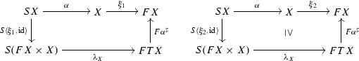
  Notice that the left model is strict, yet we can also see it as a lax model for the discrete order on F. Hence we can pair the two coalgebra structures to obtain a lax model

  

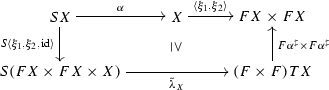  (26)

  for the monotone GSOS specification $\tilde{\lambda }$ considered above. We apply Lemma 11.5 for the lax model in (26) to obtain a lax bialgebra as in the next diagram with the carrier $(X,{\varDelta }_X)$.

  

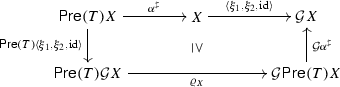
• 3. We consider the $\mathsf {Rel}^\uparrow$ lifting $\overline{\mathsf {Pre}(T)}$ of $\mathsf {Pre}(T)$ obtained using Lemma 10.10 and the $\mathsf {Rel}^\uparrow$ lifting $\overline{\mathcal {G}}$ of $\mathcal {G}$ obtained from Example 10.11. Using Proposition 14.11 in “Appendix 8” we know that the distributive law $\rho$ lifts to a distributive law $\overline{\rho }:\overline{T}\overline{G}\Rightarrow \overline{G}\overline{T}$ in $\mathsf {Rel}$. To obtain the lifting of $\overline{\varrho }$ to $\mathsf {Rel}^\uparrow$ we apply Lemma 10.12 for the liftings $\overline{T}$, $\overline{G}$, $\overline{\mathsf {Pre}(T)}$ and $\overline{\mathcal {G}}$ and the liftings $\overline{\rho }$ and $\varrho$ of $\rho$ to $\mathsf {Rel}$, respectively $\mathsf {Pre}$.

$\square$

By Remark 10.8, since the order on X is discrete, we have that $\mathsf {Rel}^\uparrow _X\cong \mathsf {Rel}_X$. Hence the functor $Ctx$ is indeed the usual predicate transformer for contextual closure and coalgebras for $(\overline{\mathsf {Pre}(F)\times \mathsf {Pre}_\subseteq (F)}\times \mathrm {Id})_{\langle \xi _1,\xi _2,\mathrm {id}\rangle }$ correspond to the usual weak bisimulations.

Example 12.2

Recall from Example 11.4 that $\rightarrow$ and $\Rightarrow$ are, respectively, a model and a lax model for the positive GSOS specification of Example 7.1. By Theorem 12.1, it follows that up-to context (for the parallel composition of CCS) is compatible for weak bisimulation.

We can apply Theorem 12.1 to prove analogous results for the other operators of CCS with the exception of $+$ which is not part of a lax model, see Example 11.4. More generally, for any process algebra specified by a positive GSOS, one simply needs to check that the saturated transistion systems is a lax model. As explained in Sect. 11, this means that whenever $\Rightarrow$ satisfies the premises of a rule, it also satisfies its consequence. By [55, Lemma WB], this holds for all calculi that conform to the so-called simply WB cool format [5], amongst which it is worth mentioning the fragment of CSP consisting of action prefixing, internal and external choice, parallel composition, abstraction and the 0 process ([55, Example 1]).

Corollary 12.3

For a simply WB cool GSOS language, up-to context is a compatible technique for weak bisimulation.

13 Simulation up-to

In this section we recall simulations for coalgebras as introduced in [25] and we restrict our attention to ordered functors as defined in Sect. 10.1. The lax relation lifting $\mathsf {Rel}_{\subseteq }(F):\mathsf {Rel}\rightarrow \mathsf {Rel}$ defined in (17) is used in [25] to give a coalgebraic characterisation of simulations. For a coalgebra $\xi :X \rightarrow FX$, the coalgebras for the endofunctor $\xi ^* \circ \mathsf {Rel}_{\subseteq }(F)_X$—which we denote by $\mathsf {Rel}_{\subseteq }(F)_{\xi }$—are called simulations. The final $\mathsf {Rel}_{\subseteq }(F)_{\xi }$-coalgebra, when it exists, is called similarity.

For instance, $\mathsf {Rel}_{\subseteq }(F)_{\xi }$-coalgebras with respect to the order defined in Example 10.3 are simulations of deterministic automata and weighted automata, while the final $\mathsf {Rel}_{\subseteq }(F)_{\xi }$-coalgebra is language inclusion. Taking instead the order in Example 10.2 one obtains the standard notions of simulations and similarity for LTSs. Since these orders are stable, the following result applies.

Proposition 13.1

If F preserves weak pullbacks and has a stable order, then $Bhv$, $Slf$, and $Trn$ are $\mathsf {Rel}_{\subseteq }(F)_{\xi }$-compatible.

Proof

Compatibility of $Bhv$ follows from Theorem 6.1. Compatibility of $Trn$ follows from Corollary 6.5. We can apply the latter since for stable ordered functors the lax relation lifting preserves relational composition by [25, Lemma 5.3], so $(*{*}*)$ holds for $\mathsf {Rel}_{\subseteq }(F)$. Similarly, the proof for the compatibility of $Slf$ relies on Lemma 6.4. $\square$

Proposition 13.2

If F, T are $\mathsf {Set}$-functors with F stable ordered and $(X, \alpha , \xi )$ is a bialgebra for a monotone $\rho :T F \Rightarrow F T$, where the orders on TF and FT are given as in Lemma 10.6, then the contextual closure functor $Ctx$ is $\mathsf {Rel}_{\subseteq }(F)_{\xi }$-compatible.

Proof

By Lemma 10.5, we obtain a natural transformation $\overline{\rho }:\mathsf {Rel}_{\subseteq }(TF)\Rightarrow \mathsf {Rel}_{\subseteq }(FT)$ above $\rho$. Using Lemma 10.6 twice, we have that $\mathsf {Rel}_{\subseteq }(TF)=\mathsf {Rel}(T)\mathsf {Rel}_{\subseteq }(F)$ and $\mathsf {Rel}_{\subseteq }(FT)=\mathsf {Rel}_{\subseteq }(F)\mathsf {Rel}(T)$, so we can see $\overline{\rho }$ as a natural transformation of type $\overline{\rho }:\mathsf {Rel}(T)\mathsf {Rel}_{\subseteq }(F) \Rightarrow \mathsf {Rel}_{\subseteq }(F)\mathsf {Rel}(T)$ sitting above $\rho$. By Theorem 6.7, it follows that $Ctx = \textstyle {\coprod }_{\alpha } \circ \mathsf {Rel}(T)$ is $\mathsf {Rel}_{\subseteq }(F)_{ \xi }$-compatible. $\square$

A similar result can be obtained when starting with models of monotone abstract GSOS specifications as defined in Sect. 11.

Proposition 13.3

Let $\lambda :S (F \times \mathrm {Id}) \Rightarrow FT$ be a monotone abstract GSOS specification and $(X, \alpha , \xi )$ be a model for $\lambda$. Then $Ctx$ is $(\mathsf {Rel}_{\subseteq }(F)\times \mathrm {Id})_{\langle \xi , \mathrm {id}\rangle }$-compatible.

Proof

As explained in Sect. 7, the model $(X, \alpha , \xi )$ yields the bialgebra $(X, \alpha ^\sharp , \langle \xi , \mathrm {id}\rangle )$ for the induced distributive law $\rho$. By Lemma 11.2 there exists a natural transformation $\varrho :\mathsf {Rel}(T)(\mathsf {Rel}_\subseteq (F)\times \mathrm {Id})\Rightarrow (\mathsf {Rel}_\subseteq (F)\times \mathrm {Id})\mathsf {Rel}(T)$, sitting above $\rho$. By Theorem 6.7, it follows that $Ctx = \textstyle {\coprod }_{\alpha ^{\sharp }} \circ \mathsf {Rel}(T)$ is $(\mathsf {Rel}_{\subseteq }(F)\times \mathrm {Id})_{\langle \xi , \mathrm {id}\rangle }$-compatible. $\square$

Example 13.4

In Sect. 2.2 we used simulation up to $Slf \circ Ctx$ to prove Arden’s rule. We can finally prove the soundness of $Slf \circ Ctx$ by exploiting the results in this section. To do so, we have to use the model $(RE',\alpha ',\xi ')$ of extended regular expressions seen in Example 11.1, rather than the standard one seen in Example 7.2, since the abstract GSOS specification for the former is monotone while the one for the latter is not.

The proof proceeds as follows. By Proposition 13.3, $Ctx$ is $(\mathsf {Rel}_{\subseteq }(F)\times \mathrm {Id})_{\langle \xi ', \mathrm {id}\rangle }$-compatible and, by Lemma 7.5, it is also $(\mathsf {Rel}_{\subseteq }(F)_{\xi '}\times \mathrm {Id})$-compatible. By Proposition 13.1, $Slf$ is $\mathsf {Rel}_{\subseteq }(F)_{\xi '}$-compatible and, by Proposition 3.4(i), it is also $(\mathsf {Rel}_{\subseteq }(F)_{\xi '}\times \mathrm {Id})$-compatible. Therefore $Slf \circ Ctx$ is $(\mathsf {Rel}_{\subseteq }(F)_{\xi '}\times \mathrm {Id})$-compatible by Proposition 3.3 and $\mathsf {Rel}_{\subseteq }(F)_{\xi '}$-sound by Proposition 3.4(iii).

14 Directions for future work

Our nominal automata example leads us to expect that the framework introduced in this paper will lend itself to obtaining a clean theory of up-to techniques for name-passing process calculi. For instance, we would like to understand whether the congruence rule format proposed by Fiore and Staton [19] can fit in our setting: this would provide general conditions under which up-to techniques related to name substitution are sound in such calculi.

Another interesting research direction is suggested by the divergence predicate we studied in Sect. 8.2. Other formulas of (coalgebraic) modal logic [17] can be expressed by taking different predicate liftings, and yield different families of compatible functors. This suggests a connection with the proof systems in [18, 48]: we can regard proofs in those systems as invariants up to some compatible functors. By using our framework and the logical distributive laws of [28], we hope to obtain a systematic way to derive or enhance such proof systems, starting from a given abstract GSOS specification.

We have shown that up-to context is compatible (and thus sound) for weak bisimulation whenever the strong and the weak transition systems are a model and a lax model for a positive GSOS specification, as it is the case for calculi adhering to the cool GSOS format [5, 55].

Using our tools, a similar result also holds for dynamic bisimilarity [36]. Indeed one can use the lifting in (14) with a different saturated transition system that is obtained as in (13) but without the axiom $x\mathop {\Rightarrow }\limits ^{\tau }x$. Then for all the rules of CCS (including $+$), whenever this system satisfies the premises, it also satisfies its consequence, so it is a lax model; hence up-to context is compatible for dynamic bisimulation.

We leave branching bisimilarity [56] and coupled simulation [37] for future work.

Our treatment of up-to techniques for weak bisimulations only covers models based on labelled transition systems. We leave as future work to integrate in our framework the coalgebraic treatment of weak bisimilarity, developed for example in [13, 14, 21] for systems modelled as colagebras in an order-enriched setting. Thus, we expect to extend our results to encompass fully probabilistic and Segala models [49, 50].

Appendices

Appendix 1: Proofs for Sect. 4

Lemma 14.1

For any functors $F,G :\mathsf {Set}\rightarrow \mathsf {Set}$, we have $\mathsf {Rel}(FG) = \mathsf {Rel}(F)\mathsf {Rel}(G)$

Proof

Recall that the canonical relation lifting $\mathsf {Rel}(G)(R)$ of a relation $i :R \hookrightarrow X \times X$ is obtained via the (epi,mono)-factorisation in (27). We assume further that all the monos in the diagrams below are inclusions.

(27)

Applying F yields the left triangle in the following diagram:

Note that Fe is an epi since $\mathsf {Set}$-functors preserve epimorphisms; this property relies on the axiom of choice. The lower right triangle is given by definition of $\mathsf {Rel}(F)(\mathsf {Rel}(G)(R))$. The upper right triangle commutes by an easy argument. By definition, $\mathsf {Rel}(FG)(R)$ is obtained by an (epi,mono)-factorisation of $\langle FG \pi _1, FG\pi _2 \rangle \circ FGi$. Since the diagram commutes and epis are closed under composition, the lower path from left to right is such an (epi,mono)-factorisation, hence $\mathsf {Rel}(FG)(R) = \mathsf {Rel}(F)(\mathsf {Rel}(G)(R))$. $\square$

Appendix 2: Proofs for Sect. 6

The next simple Lemma about liftings in fibrations will be used throughout this appendix, e.g., to prove Proposition 6.3, but also Theorem 6.7.

Lemma 14.2

Let $p:\mathcal {E}\rightarrow \mathcal {B}$ and $p':\mathcal {E}'\rightarrow \mathcal {B}$ be two fibrations and assume $\overline{T}:\mathcal {E}\rightarrow \mathcal {E}'$ is the lifting of a functor $T:\mathcal {B}\rightarrow \mathcal {B}$. Consider a $\mathcal {B}$-morphism $f:X\rightarrow Y$. Then there exists a natural transformation:

$$\begin{aligned} \theta :\overline{T}\circ f^* \Rightarrow (Tf)^*\circ \overline{T}:\mathcal {E}_Y\rightarrow \mathcal {E}'_{TX}. \end{aligned}$$

Proof

In order to define $\theta _R$ for some R in $\mathcal {E}_Y$, we use the universal property of the Cartesian lifting $\widetilde{Tf}_{\overline{T}(R)}$. In a diagram:

$\square$

Lemma 14.3

Let $p:\mathcal {E}\rightarrow \mathcal {B}$ be a bifibration and assume $\overline{F}:\mathcal {E}\rightarrow \mathcal {E}$ is the lifting of a functor $F:\mathcal {B}\rightarrow \mathcal {B}$. Consider a $\mathcal {B}$-morphism $f:X\rightarrow Y$. Then there exists a natural transformation:

$$\begin{aligned} \rho :\textstyle {\coprod }_{Ff}\circ \overline{F}\Rightarrow \overline{F}\circ \textstyle {\coprod }_f:\mathcal {E}_X\rightarrow \mathcal {E}_{FY}. \end{aligned}$$

Proof

The proof uses the universal property of the opcartesian liftings. Equivalently, from Lemma 14.2 we have a natural transformation $\theta :\overline{F}\circ f^*\Rightarrow (Ff)^*\circ \overline{F}$. Then the desired natural transformation is obtained as the so-called mate of $\theta$:

where the left-most and right-most natural transformation are given by, respectively, the unit of $\coprod _f\dashv f^*$ and the counit of $\coprod _{Ff}\dashv (Ff)^*$. $\square$

1.1 Proofs for Sect. 6.2

In this section we prove Proposition 6.3.

Lemma 14.4

Let $p:\mathcal {E}\rightarrow \mathcal {B}$ and assume $G:\mathcal {E}^{\times _{\mathcal {B}}n}\rightarrow \mathcal {E}$ is a lifting of the identity on $\mathcal {B}$. If $f:X\rightarrow Y$ is a $\mathcal {B}$-morphism, there is a canonical natural transformation

$$\begin{aligned} \theta :G(f^*)^n\Rightarrow f^*G:\mathcal {E}_Y\rightarrow \mathcal {E}_{GX}. \end{aligned}$$

Proof

This is an instance of Lemma 14.2 for $T=\mathrm {Id}$ and $\overline{T}=G$. We use that the reindexing along a $\mathcal {B}$-morphism f in $\mathcal {E}^{\times _{\mathcal {B}}n}$ is $(f^*)^n$, where $f^*$ is the Cartesian lifting in $\mathcal {E}$. (To see this, one can use the characterisation of Cartesian morphisms in fibrations obtained by change-of-base and composition, which are the basic operations used to construct the fibration $\mathcal {E}^{\times _{\mathcal {B}}^n} \rightarrow \mathcal {B}$ [26, Lemma 1.7.4].) $\square$

Proposition 6.3

Let $\overline{F}:\mathcal {E}\rightarrow \mathcal {E}$ be a lifting of a $\mathcal {B}$-functor F and $G:\mathcal {E}^{\times _{\mathcal {B}}n}\rightarrow \mathcal {E}$ be a lifting of the identity, and suppose that for each X in $\mathcal {B}$ there is a natural transformation

$$\begin{aligned} \gamma :G_{FX} \circ (\overline{F}_X)^n \Rightarrow \overline{F}_X \circ G_X : (\mathcal {E}_X)^n \rightarrow \mathcal {E}_{FX}. \end{aligned}$$

Then for any coalgebra $\xi :X \rightarrow FX$, the functor $G_X$ is $\overline{F}_{\xi }$-compatible.

Proof

We construct a natural transformation as follows:

The first equality follows from the definition of $(-)^n$ as the mediating arrow into the product $(\mathcal {E}_X)^n$. The natural transformation $\theta$ comes from Lemma 14.4. $\square$

1.2 Proofs for Sect. 6.3

Lemma 14.5

Consider a fibration $p:\mathcal {E}\rightarrow \mathcal {B}$, two $\mathcal {B}$-endofunctors F, G with corresponding liftings $\overline{F},\overline{G}$. Assume $\lambda :F\Rightarrow G$ is a natural transformation and $\overline{\lambda }:\overline{F}\Rightarrow \overline{G}$ sits above $\lambda$. Then there exist natural transformations $\overline{F}\Rightarrow \lambda _X^* \overline{G}$ and $\coprod _{\lambda _X}\overline{F}\Rightarrow \overline{G}$.

Proof

For $R\in \mathcal {E}_{FX}$ the R-component of the required natural transformation is the dashed line in (29) and is obtained using the universal property of the Cartesian lifting of $\lambda _X$.

The naturality in R can be easily checked and is a consequence of the uniqueness of the factorisation. The natural transformation $\coprod _{\lambda _X}\overline{F}R\Rightarrow \overline{G}R$ is obtained as the mate of $\overline{F}\Rightarrow \lambda _X^* \overline{G}$, that is, given by the composite

where $\varepsilon$ is the counit of the adjunction $(\coprod _\lambda \dashv \lambda ^*)$. $\square$

Lemma 14.6

Given $(X,\alpha ,\xi )$ an $\rho$-bialgebra as in (7) and $p:\mathcal {E}\rightarrow \mathcal {B}$ a fibration, there exists a 2-cell

Proof

We obtain the required natural transformation as the composite of the natural transformations of (31) below. Except for the third one, these 2-cells are obtained from the units or counits of the adjunctions recalled on the right column. The third natural transformation is actually an isomorphism and arises from $(X,\alpha ,\xi )$ being a bialgebra.

$$\begin{aligned} \begin{array}{cc} \coprod _\alpha \circ (T\xi )^* &{} \\ \Downarrow &{} (\coprod _\rho \dashv \rho ^*)\\ \coprod _\alpha \circ (T\xi )^*\circ \rho ^*\circ \coprod _{\rho } &{} \\ \Downarrow &{} (\coprod _{F\alpha }\dashv (F\alpha )^*)\\ \coprod _\alpha \circ (T\xi )^*\circ \rho ^*\circ (F\alpha )^*\circ \coprod _{F\alpha }\circ \coprod _{\rho } &{} \\ \Downarrow &{} (\mathrm {bialg})\\ \coprod _\alpha \circ \alpha ^*\circ \xi ^*\circ \coprod _{F\alpha }\circ \coprod _{\rho } &{} \\ \Downarrow &{} (\coprod _{\alpha }\dashv \alpha ^*)\\ \xi ^*\circ \coprod _{F\alpha }\circ \coprod _{\rho } &{}\square \\ \end{array} \end{aligned}$$

(31)

Appendix 3: Proofs for Sect. 7

In this section we will prove Theorem 7.4. First we recall some basic facts on the free monad T over an endofunctor S on some category $\mathcal {C}$.

Assuming S has free algebras over any X in $\mathcal {C}$ one can show that the free monad T over S exists. We can define TX as the free S-algebra on X, or equivalently, as the initial algebra for the functor $X+S(-)$. Thus for each X in $\mathcal {C}$ one has an isomorphism

$$\begin{aligned}{}[\eta _X,\kappa _X]:X+ST X\rightarrow T X. \end{aligned}$$

The $\eta$ above gives the unit of the monad T. The monad multiplication $\mu :TT X \rightarrow T X$ is defined as the unique morphism obtained by equipping TX with the algebra structure $[\mathrm {id},\kappa _X] :TX + STX \rightarrow TX$.

Recall from [54] that there exists a bijective correspondence between natural transformations

$$\begin{aligned} \lambda :S(F\times \mathrm {Id})\Rightarrow FT \end{aligned}$$

and distributive laws

$$\begin{aligned} \rho _{\lambda }:T(F\times \mathrm {Id})\Rightarrow (F\times \mathrm {Id})T. \end{aligned}$$

The natural transformation $\rho _{\lambda }$ is defined on a component X in $\mathcal {B}$ as the unique $(F\times \mathrm {Id})X + {S}(-)$-algebra morphism:

(32)

The following technical lemma is needed to establish that whenever the lifting of $\overline{S}$ of a functor S has free algebras, the free monad over $\overline{S}$ is a lifting of the free monad over S.

Lemma 14.7

Consider a lifting $\overline{S}$ of a $\mathcal {B}$-endofunctor S and assume $\overline{S}$ has free algebras.

• 1. The functor $p :\mathcal {E}\rightarrow \mathcal {B}$ has a right adjoint $\mathbf {1} :\mathcal {B}\rightarrow \mathcal {E}$ inducing an adjunction⁴

  

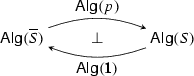
• 2. The functor $\mathsf {Alg}(p)$ preserves initial algebras.

• 3. When $P\in \mathcal {E}_X$ for some X in $\mathcal {B}$, the free $\overline{S}$-algebra over P sits above the free S-algebras over X.

• 4. The free monad $\overline{T}$ over $\overline{S}$ exists and is a lifting of the free monad T over S.

Proof

• 1. Since the fibration considered here is assumed to have fibred finite products, one can define $\mathbf {1}(X)$ as the terminal object in $\mathcal {E}_X$, and $\mathbf {1}(f :X \rightarrow Y)$ as the Cartesian lifting $\widehat{f}_{1_Y} :(1_Y)^* \rightarrow 1_Y$, which is well-defined since reindexing functors preserve terminal objects by assumption. Then the statement of this item is an immediate consequence of [23, Theorem 2.14].

• 2. follows because $\mathsf {Alg}(p)$ is a left adjoint.

• 3. follows from item 2) applied for the lifting $P+\overline{S}$ of $X+S$.

• 4. is an immediate consequence of item 3).

$\square$

Theorem 7.4

Let $(X,\alpha ,\xi )$ and $(X,\alpha ^{\sharp },\langle \xi ,\mathrm {id}\rangle )$ be a model and a bialgebra for, respectively, an abstract GSOS specification $\lambda :S(F \times \mathrm {Id}) \Rightarrow FT$ and the corresponding distributive law $\rho _{\lambda }:T(F\times \mathrm {Id}) \Rightarrow (F\times \mathrm {Id}) T$. Let $\overline{S},\overline{F}$ be liftings of S, F and assume that $\overline{S}$ has a free monad $\overline{T}$.

If there is a natural transformation $\overline{\lambda } :\overline{S}(\overline{F} \times \mathrm {Id})\Rightarrow \overline{F}\overline{T}$ sitting above $\lambda$, then

• 1. there exists $\overline{\rho _{\lambda }} :\overline{T}\,(\overline{F} \times \mathrm {Id})\Rightarrow (\overline{F} \times \mathrm {Id})\overline{T}$ sitting above $\rho _{\lambda }$;

• 2. $\textstyle {\coprod }_{\alpha ^\sharp } \circ {\overline{T}}$ is $(\overline{F}\times \mathrm {Id})_{\langle \xi ,\mathrm {id}\rangle }$-compatible.

Proof

We know that TX is the free S-algebra on X. Let

$$\begin{aligned}{}[\eta _X,\kappa _X]:X+{S}{T} X\rightarrow {T} X \end{aligned}$$

denote the initial $X+{S}(-)$-algebra. Similarly, given P in $\mathcal {E}_X$, let

$$\begin{aligned}{}[\overline{\eta }_P,\overline{\kappa }_P]:P+\overline{S}\,\overline{{T}} P\rightarrow \overline{{T}} P \end{aligned}$$

denote the initial $P+\overline{S}(-)$-algebra. By Lemma 14.7 we know that $[\overline{\eta }_P,\overline{\kappa }_P]$ is a lifting of $[\eta _X,\kappa _X]$.

For $P\in \mathcal {E}_X$ the map $\overline{\rho _{\lambda }}_P$ is defined as in (32), as the unique map in the following diagram:

(33)

By Lemma 14.7 we have that the $(\overline{F}\times \mathrm {Id})P + \overline{S}(-)$-algebras $\overline{{T}} (\overline{F}\times \mathrm {Id})P$ and $(\overline{F}\times \mathrm {Id})\overline{{T}} P$ of diagram (33) sit above the $(F\times \mathrm {Id})X + {S}(-)$-algebras $T(F\times \mathrm {Id}) X$, respectively $(F\times \mathrm {Id}){T} X$ of diagram (32). By uniqueness of $\rho _{\lambda }{}_X$ it follows that $\overline{\rho _{\lambda }}_P$ sits above $\rho _{\lambda }{}_X$. $\square$

Lemma 7.7

Let $S, \overline{S}$, T and $\overline{T}$ be as in Theorem 7.4. Given an algebra $\alpha :S X \rightarrow X$ with induced algebra $\alpha ^\sharp :T X \rightarrow X$ for the free monad T, there exists a natural transformation of the form $\textstyle {\coprod }_{\alpha } \circ \overline{S} \Rightarrow \textstyle {\coprod }_{\alpha ^\sharp } \circ \overline{T}$.

Proof

Let $\eta :\mathrm {Id}\Rightarrow T$ and $\kappa :S T \Rightarrow T$ be the canonical natural transformations defined by initiality (see “Appendix 3”); composing them yields a natural transformation $\iota :S \Rightarrow T$. Similarly, we can construct a natural transformation $\overline{\iota } :\overline{S} \Rightarrow \overline{T}$ above $\iota$.

The desired natural transformation consists of two pieces:

• (a) Since $\overline{\iota }$ sits above $\iota$, the desired natural transformation exists by Lemma 14.5.

• (b) We have $\alpha = \alpha ^\sharp \circ \iota _X$, so ${\textstyle {\coprod }}_{\alpha } = {\textstyle {\coprod }}_{\alpha ^\sharp \circ \iota _X} \cong {\textstyle {\coprod }}_{\alpha ^\sharp } \circ {\textstyle {\coprod }}_{\iota _X}$.

$\square$

Appendix 4: Proofs for Sect. 8

1.1 Weighted language inclusion

Using the notations of Sect. 8.1, in this appendix we first prove that for a semiring $\mathbb {S}$ satisfying conditions (a) and (b) on page 31 we have:

$$\begin{aligned} (\rho _X \times \rho _X)(\mathsf {Rel}(\mathbb {S}^-_\omega )(\overline{F}(R))) \subseteq \overline{F}(\mathsf {Rel}(\mathbb {S}^-_\omega )(R)) \end{aligned}$$

(34)

for any relation $R \subseteq X \times X$ and any X. First, we compute $\mathsf {Rel}(\mathbb {S}^-_\omega ) (\overline{F}(R))$:

$$\begin{aligned} \left\{ \left( \sum r_i (p_i,\varphi _i), \sum r_i (q_i, \psi _i)\right) \mid \forall i. \, p_i \le q_i \text { and } \forall a. \, (\varphi _i(a), \psi _i(a)) \in R \right\} \end{aligned}$$

Applying $\rho _X \times \rho _X$ yields a relation on $F \mathbb {S}^-_\omega X$:

$$\begin{aligned}&\left\{ \left( \left( \sum r_i \cdot p_i, \lambda a. \sum r_i \cdot \varphi _i(a)\right) , \left( \sum r_i \cdot q_i, \lambda a. \sum r_i \cdot \psi _i(a)\right) \right) \right. \\&\left. \qquad \mid \forall i. \, p_i \le q_i \text { and } \forall a.\, (\varphi _i(a),\psi _i(a)) \in R \phantom {(\sum }\right\} \end{aligned}$$

Now we compute $\overline{F}(\mathsf {Rel}(\mathbb {S}^-_\omega )(R))$:

$$\begin{aligned} \left\{ \left( \left( p, a \mapsto \sum r_{a,i} x_{a,i}\right) , \left( q, a \mapsto \sum r_{a,i} y_{a,i}\right) \right) \mid p \le q \text { and } \forall a. \, \forall i. \, (x_{a,i},y_{a,i}) \in R \right\} \end{aligned}$$

It follows that the inclusion (34) holds whenever $\sum r_i \cdot p_i \le \sum r_i \cdot q_i$ given that $p_i \le q_i$ for all i. Hence, it suffices that the operations $+$ and $\cdot$ are monotone with respect to the order $\le$ on the semiring.

Now we turn to the last example of Sect. 8.1, involving the semiring $\mathbb {R}$, which does not satisfy the condition (b) on page 31. For the monotone contextual closure, we prove the inclusion $(\rho _X \times \rho _X)(\overline{\mathbb {R}^-_\omega } (\overline{F} (R))) \subseteq \overline{F} (\overline{\mathbb {R}^-_\omega }(R))$, for the lifting $\overline{\mathbb {R}^-_\omega }$ defined in Equation 12. First, we compute $\overline{\mathbb {R}^-_\omega }(\overline{F}(R))$:

$$\begin{aligned} \left\{ \left( \sum r_i (p_i,\varphi _i), \sum r_i (q_i, \psi _i)\right) \mid \forall i. \begin{array}{lcr} r_i \ge 0 &{}\Rightarrow &{}p_i \le q_i \text { and } \forall a. \varphi _i(a) \mathrel {R} \psi _i(a)) \\ r_i < 0 &{}\Rightarrow &{}q_i \le p_i \text { and } \forall a. \psi _i(a) \mathrel {R} \varphi _i(a)) \\ \end{array}\right\} \end{aligned}$$

Then $(\rho _X \times \rho _X)(\overline{\mathbb {R}^-_\omega } (\overline{F} (R)))$ is:

$$\begin{aligned}&\left\{ \left( \left( \sum r_i \cdot p_i, a \mapsto \sum r_i \cdot \varphi _i(a)\right) , \left( \sum r_i \cdot q_i, a \mapsto \sum r_i \cdot \psi _i(a)\right) \right) \right. \\&\qquad \left. \mid \forall i. \begin{array}{r} r_i \ge 0 \Rightarrow p_i \le q_i \text { and } \forall a. (\varphi _i(a),\psi _i(a)) \in R \\ r_i < 0 \Rightarrow q_i \le p_i \text { and } \forall a. (\psi _i(a),\varphi _i(a)) \in R \\ \end{array} \right\} \end{aligned}$$

Finally $\overline{F} (\overline{\mathbb {R}^-_\omega }(R))$ is

$$\begin{aligned} \left\{ \left( \left( p, a \mapsto \sum r_{a,i} x_{a,i}\right) , \left( q, a \mapsto \sum r_{a,i} y_{a,i}\right) \right) \mid p \le q; \forall a. \forall i. \begin{array}{r} r_{a,i} \ge 0 \Rightarrow (x_{a,i},y_{a,i}) \in R \\ r_{a,i} < 0 \Rightarrow (y_{a,i}, x_{a,i}) \in R \end{array} \right\} \end{aligned}$$

The desired inclusion holds, since $r_i \cdot p_i \le r_i \cdot q_i$ for all i. The reason is that $p_i \le q_i$ when $r_i \ge 0$, whereas $q_i \le p_i$ if $r_i < 0$.

1.2 Nominal automata

In this section we assume the reader has some familiarity with nominal sets, see [39].

1.2.1 The base category

We denote by $\mathbb {A}$ a countable set of names. The category $\mathsf {Nom}$ of nominal sets has as objects sets X equipped with an action $\cdot : Sym (\mathbb {A})\times X\rightarrow X$ of the group of finitely supported permutations on $\mathbb {A}$ (that is, permutations generated by transpositions of the form $(a\ b)$) and such that each $x\in X$ has a finite support. Morphisms in $\mathsf {Nom}$ are equivariant functions, i.e., functions that preserve the group action.

1.2.2 The fibration at issue

It is well known that $\mathsf {Nom}$ can equivalently be described as a Grothendieck topos. Since $\mathsf {Nom}$ is a regular category, by [26, Observation 4.4.1] we know that the subobject fibration on $\mathsf {Nom}$ is in fact a bifibration. Furthermore, by a change-of-base situation described below we obtain the bifibration $\mathsf {Rel}(\mathsf {Nom})\rightarrow \mathsf {Nom}$, see also [26, Example 9.2.5(ii)]

Objects of $\mathsf {Rel}(\mathsf {Nom})$ are equivariant relations. That is, if X is a nominal set, a nominal relation on X is just a subset $R\subseteq X^2$ such that xR y implies $(\pi \cdot x) R(\pi \cdot y)$ for all permutations $\pi$. This bifibration is also split and bicartesian.

1.2.3 The functors and the distributive law

We will use the following $\mathsf {Nom}$-endofunctors:

• 1. $F:\mathsf {Nom}\rightarrow \mathsf {Nom}$ given by $FX=2\times X^\mathbb {A}$, where $2=\{0,1\}$ is equipped with the trivial action and $X^\mathbb {A}$ is given by the internal hom. Concretely, an element $f\in X^\mathbb {A}$ is a function $f:\mathbb {A}\rightarrow X$ such that there exists a finite subset $S\subseteq \mathbb {A}$ and $f(\pi (a))=\pi \cdot f(a)$ for all names $a\in \mathbb {A}$ and permutations $\pi \in Sym (\mathbb {A})$ fixing the elements of S.

• 2. $\mathcal {P}_{\omega }:\mathsf {Nom}\rightarrow \mathsf {Nom}$ that maps a nominal set X to its orbit-finite finitely supported subsets. In particular one can check that $\mathcal {P}_{\omega }$ is a monad and let $\mu$ denote its multiplication, given by union.

The functors $\mathcal {P}_{\omega }$ and F are related by a distributive law

$$\begin{aligned} \lambda :\mathcal {P}_{\omega }F\Rightarrow F\mathcal {P}_{\omega }. \end{aligned}$$

For a nominal set X, the map $\lambda _X$ is given by the product of the morphisms acting on $S\in \mathcal {P}_{\omega }F(X)$ by

$$\begin{aligned} S \mapsto 1\in 2\quad \mathrm {\ iff\ } 1\in (\mathcal {P}_{\omega }\tau _1)(S) \end{aligned}$$

and

$$\begin{aligned} S \mapsto \lambda a.\{x\in X | \exists f\in (\mathcal {P}_{\omega }\tau _2)(S).\ f(a)=x\}\in (\mathcal {P}_{\omega }X)^A \end{aligned}$$

where $\tau _1,\tau _2$ are the projections from FX to 2, respectively $X^\mathbb {A}$.

1.2.4 The liftings

The distributive law $\lambda$ can be lifted to $\mathsf {Rel}(\mathsf {Nom})$, see [27, Exercise 4.4.6].

$$\begin{aligned} \mathsf {Rel}(\lambda ):\mathsf {Rel}(\mathcal {P}_{\omega }) \mathsf {Rel}(F)\Rightarrow \mathsf {Rel}(F)\mathsf {Rel}(\mathcal {P}_{\omega }). \end{aligned}$$

using the fact that, in this case $\mathsf {Rel}(\mathcal {P}_{\omega }) \mathsf {Rel}(F)=\mathsf {Rel}(\mathcal {P}_{\omega }F)$ and $\mathsf {Rel}(F) \mathsf {Rel}(\mathcal {P}_{\omega })=\mathsf {Rel}(F\mathcal {P}_{\omega })$. Concretely, for $R\in \mathsf {Rel}(\mathsf {Nom})_X$, the nominal relation $\mathsf {Rel}(F)(R)$ is given by $(o,f)\ \mathsf {Rel}(F)(R)\ (o',f')$ iff $o=o'$ and for all $a\in \mathbb {A}$ we have $f(a) Rf'(a)$.

On the other hand $\mathsf {Rel}(\mathcal {P}_{\omega })$ is given by $S\ \mathsf {Rel}(\mathcal {P}_{\omega })(R)\ S'$ iff for all $x\in S$ exists $y\in S'$ with xRy and for all $y\in S'$ exists $x\in S$ with xRy. As for $\mathsf {Rel}(\lambda )_R$, this is obtained as the restriction of $\lambda _R\times \lambda _R$ to $\mathsf {Rel}(\mathcal {P}_{\omega }) \mathsf {Rel}(F)(R)$.

1.2.5 Soundness of bisimulation up to congruence

Nondeterministic nominal automata [7] can be modelled as $F\mathcal {P}_{\omega }$-coalgebras, while deterministic nominal automata are represented as F-coalgebras. The classical notion of finiteness is replaced by orbit-finiteness—from a categorical perspective this makes sense, since orbit-finite nominal sets are exactly the finitely presentable objects in the lfp category $\mathsf {Nom}$.

The generalised powerset construction [47] can be applied in this situation as well, that is, a nondeterministic nominal automata modelled as a coalgebra

$$\begin{aligned} \langle o,t \rangle :X\rightarrow 2\times \mathcal {P}_{\omega }(X)^A \end{aligned}$$

yields an F-coalgebra structure

$$\begin{aligned} \langle o^\sharp ,t^\sharp \rangle :\mathcal {P}_{\omega }X\rightarrow 2\times (\mathcal {P}_{\omega }X)^A, \end{aligned}$$

on $\mathcal {P}_{\omega }X$, given by the composite $F(\mu ) \circ \lambda \circ \mathcal {P}_{\omega }(\langle o,t \rangle )$. The reason why determinisation fails in a nominal setting [7] is that the finitary power object functor $\mathcal {P}_{\omega }$ does not preserve orbit finiteness. This is the case in the example of Sect. 8.3.

Notice that $(\mathcal {P}_{\omega }X, \mu , \langle o^\sharp ,t^\sharp \rangle )$ is a $\lambda$-bialgebra.

The fibrations $\mathsf {Rel}(\mathsf {Nom})\rightarrow \mathsf {Nom}$ and $\mathsf {Sub}(\mathsf {Nom})\rightarrow \mathsf {Nom}$ are well-founded in the sense of [22]. To prove this we can apply [22, Lemma 3.4], which gives as a sufficient condition for well-foundedness: that the fibre above each finitely presentable object be finite. Indeed, recall from [38] that finitely presentable nominal sets are the orbit-finite ones. Then, it is easy to check that a nominal set with n orbits has $2^n$ equivariant nominal subsets.

Hence, by [Theorem 3.7][22], the final $\mathsf {Rel}(F)_{\langle o,t \rangle }$-coalgebra exists and can be computed as the limit of an $\omega ^ op$-chain in the fibre $\mathsf {Rel}(\mathsf {Nom})_X$. We will use this coinductive predicate to prove that two states of a nominal automata accept the same language.

We can apply Theorem 6.7 to prove that the contextual closure $Ctx =\coprod _\mu \circ \mathsf {Rel}(\mathcal {P}_{\omega })$ is $\mathsf {Rel}(F)_{\langle o^{\sharp },t^{\sharp } \rangle }$-compatible.

Thus bisimulation up to context is a valid proof technique for nominal automata.

Moreover, we can apply Proposition 6.3 to prove compatibility of the up to reflexive, symmetric and transitive closure techniques, respectively.

$(n{=}0)$ :

Let $Dia :\mathsf {Nom}\rightarrow \mathsf {Rel}(\mathsf {Nom})$ be the functor mapping each nominal set X to ${\varDelta }_X$, the diagonal relation on X. Then $Dia _X$ is $\mathsf {Rel}(F)_{\langle o,t \rangle }$-compatible since ${\varDelta }_{FX}= \mathsf {Rel}(F){\varDelta }_X$.

$(n{=}1)$ :

Let $Inv :\mathsf {Rel}(\mathsf {Nom})\rightarrow \mathsf {Rel}(\mathsf {Nom})$ be the functor mapping each nominal relation $R\subseteq X^2$ to its converse $R^{-1}\subseteq X^2$. $Inv _X$ is $\overline{F}_{\langle o,t \rangle }$-compatible since $\overline{F}(R)^{-1} \subseteq \overline{F}(R^{-1})$ for all relations $R\subseteq X^2$.

$(n{=}2)$ :

Let $\otimes :\mathsf {Rel}(\mathsf {Nom})\times _\mathsf {Nom}\mathsf {Rel}(\mathsf {Nom})\rightarrow \mathsf {Rel}(\mathsf {Nom})$ be the nominal relational composition functor. Composition of nominal relations is computed just as in $\mathsf {Set}$ and one can show that $\mathsf {Rel}(F)$ preserves it. Thus $\otimes$ is $\mathsf {Rel}(F)_{\langle o,t \rangle }$-compatible.

Employing Proposition 3.3 and the fact that congruence closure is obtained as the composition of the equivalence, context and reflexive closure functors we derive that bisimulation up to congruence is a sound technique.

1.2.6 The concrete example

The nondeterministic nominal automaton of Sect. 8.3 (reported on the left below) is given formally by an $F\mathcal {P}_{\omega }$-coalgebra $\langle o,t \rangle$ on the nominal set $1+1+\mathbb {A}+\mathbb {A}+1$. For simplicity we denote the second copy of $\mathbb {A}$ by $\mathbb {A}'$. The map $\langle o,t \rangle$ is given below on the right.

The determinisation of this automaton has infinitely many orbits. For example, the determinisation of the part reachable from $*$ is partially represented by

However, we can prove that $*$ and $\star$ accept the same language, showing that the nominal relation R spanned by

$$\begin{aligned} (\{*\},\{\star \}),~ (\{a\},\{a,a'\}),~ (\{\top \},\{ a,\top \}),~ (\{*\},\mathbb {A}') \end{aligned}$$

is a bisimulation up to congruence, that is, $R\subseteq \mathsf {Rel}(F)_{\langle o^{\sharp },t^{\sharp } \rangle } Cgr (R)$.

Fig. 3

Proving R to be a bisimulation up to congruence

This is shown in Fig. 3: for each pair in R, we check that the successors are in $Cgr (R)$. Note that for the pairs $(\{a\},\{a,a'\})$ and $(\{\top \},\{ a,\top \})$, in the second and third rows, one needs to check the successors for a and for a fresh name b. Instead for the pairs $(\{*\},\{\star \})$ and $(\{*\},\mathbb {A}')$ in the first row, only successors for a should be checked (since a does not belong to the support of these states).

The only non-trivial computation is to check whether $\{*,a\} Cgr (R) \{a\}\cup (\mathbb {A}'\setminus \{a'\})$. We proceed as follows:

$$\begin{aligned} \begin{array}{lcl} \{*,a\} &{} Cgr (R) &{} \{a\}\cup \mathbb {A}' \\ &{} Cgr (R) &{}\{a,a'\}\cup (\mathbb {A}'\setminus \{a'\})\\ &{} Cgr (R) &{} \{a\}\cup (\mathbb {A}'\setminus \{a'\}).\\ \end{array} \end{aligned}$$

Appendix 5: Proofs for Sect. 9

Lemma 14.8

$(\overline{F \times F}, F)$ is a fibration map.

Proof

Let $f:X \rightarrow Y$ be a function and $R\subseteq X^2$ be a relation. Then

$$\begin{aligned}&\overline{F \times F} ((f \times f^{-1}(R)) \\&= \{(S,U,V,W) \mid \\&\qquad \begin{array}{ll} \forall (a,x) \in S.~\exists (a,y) \in W.~f(x) R f(y),\\ \forall (a,y) \in V.~\exists (a,x) \in U.~f(x) R f(y) \} \end{array} \\&= \{(S,U,V,W) \mid \\&\qquad \begin{array}{ll} \forall (a,x') \in Ff[S].~\exists (a,y') \in Ff[W].~x' R y',\\ \forall (a,y') \in Ff[V].~\exists (a,x') \in Ff[U].~x' R y' \} \end{array} \\&= (Ff \times Ff \times Ff \times Ff)^{-1}(\overline{F \times F}(R)) \end{aligned}$$

$\square$

Appendix 6: Proofs for Sect. 10

Proof of Lemma 10.9

Since $\mathsf {Rel}^\uparrow _Y$ is a poset we have to show that for every up-closed relation $S\subseteq Y^2$ we have $f^*S\subseteq g^*S$. Consider $(x,y)\in f^*S$. Then $(f(x),f(y))\in S$. Since S is up-closed, $f(x)\le g(x)$ and $f(y)\le g(y)$ we get that $(g(x),g(y))\in S$, or equivalently, $(x,y)\in g^*S$. $\square$

Proof of Lemma 10.10

We have to prove that $\mathsf {Rel}(T)$ restricts to up-closed relations. Indeed, consider an up-closed relation $R\in \mathsf {Rel}^\uparrow _{(X,\le )}$ on X. This means that $\le ^ op \otimes R\otimes \le \subseteq R$, where $\le ^ op$ is the reverse of the order $\le$. Since $\mathsf {Rel}(T)$ preserves relation composition for weak pullback preserving functors, we derive that $\mathsf {Rel}(T)(\le ^ op )\otimes \mathsf {Rel}(T)(R)\otimes \mathsf {Rel}(T)(\le )\subseteq \mathsf {Rel}(T)(R)$. Using that $\mathsf {Rel}(T)(\le ^ op )=\mathsf {Rel}(T)(\le )^ op$ and that the order on $\mathsf {Pre}(T)(X,\le )$ is precisely $\mathsf {Rel}(T)(\le )$ we conclude that $\mathsf {Rel}(T)(R)$ is an up-closed relation on $\mathsf {Pre}(T)(X,\le )$. $\square$

Details for Example 10.11

Assume we have the following situation

This means that for all $a\in L$ we have the following

$$\begin{aligned} \begin{aligned}&\forall x\in f(a).\ \exists y\in h(a). x \le y \\ (f,g) \ \mathsf {Rel}(F)(\le )\times \mathsf {Rel}_\subseteq (F)(\le )\ (h,k)\Leftrightarrow & {} \forall y\in h(a).\ \exists x\in f(a). x \le y \\&\forall x\in g(a).\ \exists y\in k(a). x \le y \\&\\ (f,g) \ \overline{F\times F}(R)\ (f',g')\Leftrightarrow & {} \forall x\in f(a).\ \exists y\in g'(a). x R y \\&\forall x\in f'(a).\ \exists y\in g(a). x R y \\&\\&\forall x\in f'(a).\ \exists y\in h'(a). x \le y \\ (f',g') \ \mathsf {Rel}(F)(\le )\times \mathsf {Rel}_\subseteq (F)(\le )\ (h',k')\Leftrightarrow & {} \forall y\in h'(a).\ \exists x\in f'(a). x \le y \\&\forall x\in g'(a).\ \exists y\in k'(a). x \le y \\ \end{aligned} \end{aligned}$$

(35)

and we need to show

$$\begin{aligned} \begin{aligned} \forall x\in h(a).\ \exists y\in k'(a). x R y \\ \forall x\in h'(a).\ \exists y\in k(a). x R y \\ \end{aligned} \end{aligned}$$

(36)

Using the fact the R is up-closed we can prove this using (35). $\square$

Remark 14.9

Notice that some of the relations in (35) were not actually used in the proof. In order for the lifting $\overline{F\times F}(R)$ to restrict to up-closed relations, we need to carefully choose the $\mathsf {Pre}$-liftings for $F\times F$. Indeed, we could replace the lifting $\mathsf {Pre}(F)$ with the lax relation lifting given by pointwise reverse inclusion $\mathsf {Pre}_\supseteq (F)$. However the proof would break if we would consider instead the $\mathsf {Pre}$-lifting of $F\times F$ given by $\mathsf {Pre}_\subseteq (F)\times \mathsf {Pre}_\subseteq (F)$, since the functor $\mathsf {Pre}_\subseteq (F)\times \mathsf {Pre}_\subseteq (F)$ does not have a $\mathsf {Rel}^\uparrow$ lifting that also extends $\overline{F\times F}$.

Proof of Lemma 10.12

We have that $\varrho$ lifts to $\overline{\varrho }:\overline{\mathcal {T}}\overline{\mathcal {F}}\Rightarrow \overline{\mathcal {F}}\overline{\mathcal {T}}$ if and only if for any $R\in \mathsf {Rel}^\uparrow _X$ we have

$$\begin{aligned} \overline{\mathcal {T}}\overline{\mathcal {F}}(R)\subseteq \varrho ^*_X(\overline{\mathcal {F}}\overline{\mathcal {T}}(R)). \end{aligned}$$

(37)

We will show that the following inclusions are equivalent:

$$\begin{aligned} \begin{aligned} \begin{array}{lcrcl} \overline{\mathcal {T}}\overline{\mathcal {F}}(R)\subseteq \varrho ^*_X(\overline{\mathcal {F}}\overline{\mathcal {T}}(R))&{} \Leftrightarrow &{} \overline{U} \overline{\mathcal {T}}\overline{\mathcal {F}}(R) &{}\subseteq &{} \overline{U}\varrho ^*_X\overline{\mathcal {F}}\overline{\mathcal {T}}(R) \\ &{} \Leftrightarrow &{} \overline{U} \overline{\mathcal {T}}\overline{\mathcal {F}}(R) &{}\subseteq &{} \rho ^*_X\overline{U}\overline{\mathcal {F}}\overline{\mathcal {T}}(R) \\ &{} \Leftrightarrow &{} \overline{T}\overline{F}(\overline{U}R) &{}\subseteq &{} \rho ^*_X\overline{F}\overline{T}(\overline{U}R) \\ \end{array} \end{aligned} \end{aligned}$$

(38)

The first equivalence is valid because an inclusion holds in $\mathsf {Rel}^\uparrow$ iff it holds in $\mathsf {Rel}$. The second equivalence follows from the fact that $\overline{U}\varrho ^*_X=\rho ^*_X$. The last equivalence above holds because, by hypothesis, we have $\overline{U\mathcal {T}}=\overline{T}\overline{U}$ and $\overline{U\mathcal {F}}=\overline{F}\overline{U}$.

To conclude, notice that the last inclusion in (38) holds because $\rho$ can be lifted to a distributive law $\overline{\rho }$ between $\mathsf {Rel}$-functors. $\square$

Appendix 7: Proofs for Sect. 11

Lemma 10.6

Suppose $F:\mathsf {Set}\rightarrow \mathsf {Set}$ has a stable order given by a factorisation through $F_{\subseteq }:\mathsf {Set}\rightarrow \mathsf {Pre}$ and let $G:\mathsf {Set}\rightarrow \mathsf {Set}$ be a weak pullback preserving functor. Then the $\mathsf {Set}$-functors $F\times \mathrm {Id}$, GF and FG have stable orders given by:

(19)

where $D :\mathsf {Set}\rightarrow \mathsf {Pre}$ is the functor assigning to a set the discrete order (Remark 10.8) and $\mathsf {Pre}(G)$ is the canonical $\mathsf {Pre}$-lifting of G. Moreover, the lax relation and $\mathsf {Pre}$-liftings of these ordered functors satisfy:

$$\begin{aligned} \begin{array}{lll} &{}\mathsf {Rel}_\subseteq (F\times \mathrm {Id})=\mathsf {Rel}_\subseteq (F)\times \mathrm {Id}\qquad \qquad &{} \quad \qquad \mathsf {Pre}_\subseteq (F\times \mathrm {Id})=\mathsf {Pre}_\subseteq (F)\times \mathrm {Id}\\ &{}\mathsf {Rel}_\subseteq (GF)=\mathsf {Rel}(G)\mathsf {Rel}_\subseteq (F) &{} \quad \qquad \mathsf {Pre}_\subseteq (GF)=\mathsf {Pre}(G)\mathsf {Pre}_\subseteq (F)\\ &{}\mathsf {Rel}_\subseteq (FG)=\mathsf {Rel}_\subseteq (F)\mathsf {Rel}(G)&{} \quad \qquad \mathsf {Pre}_\subseteq (FG)=\mathsf {Pre}_\subseteq (F)\mathsf {Pre}(G) \end{array} \end{aligned}$$

(20)

Proof

The diagrams (19) clearly commute. Before proving that the orders are stable, we prove that the lax relation liftings are computed in a compositional way, i.e., that the equations in the second part of the statement are satisfied.

• 1. The order on $F\times \mathrm {Id}$ given in the leftmost diagram of (19) yields a constant relation lifting $\overline{\subseteq }\times {\varDelta }$ of $F\times \mathrm {Id}$, defined on the fibre above X by $\subseteq _X\times {\varDelta }_X$, where ${\varDelta }_X$ is as before the diagonal on X. Using certain properties of the canonical relation lifting (Lemma 4.7) and of relational composition $\otimes$ we obtain

  $$\begin{aligned} \mathsf {Rel}_\subseteq (F\times \mathrm {Id}) \qquad= & {} (\overline{\subseteq }\times {\varDelta }) \otimes \mathsf {Rel}(F\times \mathrm {Id})\otimes (\overline{\subseteq }\times {\varDelta }) \\= & {} (\overline{\subseteq }\times {\varDelta })\otimes (\mathsf {Rel}(F)\times \mathrm {Id}) \otimes (\overline{\subseteq }\times {\varDelta }) \\= & {} (\overline{\subseteq }\otimes \mathsf {Rel}(F)\otimes \overline{\subseteq }) \times ({\varDelta }\otimes \mathrm {Id}\otimes {\varDelta }) \\= & {} \mathsf {Rel}_\subseteq (F)\times \mathrm {Id}\end{aligned}$$

• 2. The order on GF induced by the second diagram of of (19) yields a constant relation lifting on GF, defined on a fibre above X by $\mathsf {Pre}(G)(\subseteq _{FX})$ Recall that since G preserves weak pullbacks the $\mathsf {Pre}$-lifting $\mathsf {Pre}(G)$ was defined as the restriction of $\mathsf {Rel}(G)$ to preorders. So the constant relational lifting of GF can be equivalently written as $(\mathsf {Rel}(G)\circ \overline{\subseteq })$. Using that $\mathsf {Rel}(G)$ preserves relational composition (see Lemma 4.7) we get

  $$\begin{aligned} \mathsf {Rel}_\subseteq (GF) \qquad= & {} (\mathsf {Rel}(G)\circ \overline{\subseteq })\otimes \mathsf {Rel}(GF) \otimes (\mathsf {Rel}(G)\circ \overline{\subseteq }) \\= & {} (\mathsf {Rel}(G)\circ \overline{\subseteq })\otimes (\mathsf {Rel}(G)\circ \mathsf {Rel}(F)) \otimes (\mathsf {Rel}(G)\circ \overline{\subseteq }) \\= & {} \mathsf {Rel}(G)\circ (\overline{\subseteq }\otimes \mathsf {Rel}(F) \otimes \overline{\subseteq }) \\= & {} \mathsf {Rel}(G)\circ \mathsf {Rel}_\subseteq (F) \end{aligned}$$

• 3. The order on FG coming from the rightmost diagram in (19) is given on the fibre above X by the constant $\subseteq _{GX}$. This relational lifting can be equivalently written as $\overline{\subseteq }\circ \mathsf {Rel}(G)$. We thus have

  $$\begin{aligned} \mathsf {Rel}_{\subseteq }(FG) \qquad= & {} (\overline{\subseteq }\circ \mathsf {Rel}(G))\otimes \mathsf {Rel}(FG)\otimes (\overline{\subseteq }\circ \mathsf {Rel}(G) \\= & {} (\overline{\subseteq }\circ \mathsf {Rel}(G))\otimes (\mathsf {Rel}(F)\circ \mathsf {Rel}(G))\otimes (\overline{\subseteq }\circ \mathsf {Rel}(G) \\= & {} (\overline{\subseteq }\otimes \mathsf {Rel}(F)\otimes \overline{\subseteq }) \circ \mathsf {Rel}(G) \\= & {} \mathsf {Rel}_\subseteq (F) \circ \mathsf {Rel}(G) \end{aligned}$$

Since the order on F is stable it follows that $\mathsf {Rel}_\subseteq (F)$ is a fibred functor. Since G is weak pullback preserving, so is $\mathsf {Rel}(G)$. Since fibred functors are closed under composition and multiplication with $\mathrm {Id}$ it follows that the lax relation liftings $\mathsf {Rel}_{\subseteq }(F\times \mathrm {Id})$, $\mathsf {Rel}_{\subseteq }(GF)$ and $\mathsf {Rel}_{\subseteq }(FG)$ are fibred functors. This implies that the orders in (19) are stable. Hence these relation liftings restrict the lax $\mathsf {Pre}$-liftings, and the equalities in the second column of (20) immediately follow. $\square$

Lemma 14.10

Let S be a $\mathsf {Set}$-functor such that for every set X, the initial algebra $\mu Y.(X+SY)$ exists. Then it is well known that the free monad T over S exists and is given by $TX=\mu Y.(X+SY)$. Then the canonical relation lifting $\mathsf {Rel}(T)$ of the free monad over T is the free monad over $\mathsf {Rel}(S)$. Moreover, if $\mathsf {Rel}(S)$ restricts to $\mathsf {Pre}$ then so does $\mathsf {Rel}(T)$.

Proof

For the first part we show that for every $R\subseteq X^2$ in $\mathsf {Rel}$ the initial algebra of the functor $R+\mathsf {Rel}(S)(-)$ is given by $\mathsf {Rel}(T)(R)$. In order to give the algebra map

$$\begin{aligned} R+\mathsf {Rel}(S)\mathsf {Rel}(T)(R)\rightarrow \mathsf {Rel}(R) \end{aligned}$$

(39)

recall that $\mathsf {Rel}(S)\mathsf {Rel}(T)=\mathsf {Rel}(ST)$ and use the notations $\eta$ and $\mu$ for the unit and multiplication of T. We will also denote by $\iota :S\Rightarrow T$ the canonical natural transformation exhibiting T as the free monad over S. Then the map (39) is given by the coproduct of the maps $\mathsf {Rel}(\eta )_R:R\rightarrow \mathsf {Rel}(T)(R)$ and $\mathsf {Rel}(\mu \circ \iota T)_R:Rel(ST)(R)\rightarrow \mathsf {Rel}(T)(R)$. Notice that the map (39) sits above the $\mathsf {Set}$ morphism $X+STX\rightarrow TX$ which gives the initial algebra structure on TX.

Now assume $U\subseteq V^2$ is another relation carrying a $R+\mathsf {Rel}(S)(-)$-algebra structure. This means that we have a $X+S(-)$-algebra structure on V, say $[f,g]:X+SV\rightarrow V$, such that $[f,g]\times [f,g]$ restricts to a morphism

$$\begin{aligned} R+\mathsf {Rel}(S)(U)\rightarrow U \end{aligned}$$

Since TX is the initial $X+S(-)$-algebra it suffices to show that the induced algebra morphism $h:TX\rightarrow V$ gives rise to a morphism of $R+\mathsf {Rel}(S)(-)$-algebras, that is, that h underlies a morphism $\mathsf {Rel}(T)(R)\rightarrow U$, so that we get the following diagram

(40)

The map $g:SV\rightarrow V$ has a unique extension to TV, that is, we have $\overline{g}:TV\rightarrow V$ such that $\overline{g}\iota _V=g$. Then the map $h:TX\rightarrow V$ is obtained as the composite of $Tf:TX\rightarrow TV$ and $\overline{g}:TV\rightarrow V$, i.e., $h=\overline{g}\circ Tf$. The map Tf underlines a morphism of relations $\mathsf {Rel}(T)(R)\rightarrow \mathsf {Rel}(T)(U)$, simply because f underlines a morphism of relations $R\rightarrow U$. So it suffices to show that the map $\overline{g}$ underlines a morphism of relations $\mathsf {Rel}(T)(U)\rightarrow U$. Then it follows that h gives rise to a morphism $\mathsf {Rel}(T)(R)\rightarrow U$ as in the diagram above. Hence it just remains to prove that the next diagram holds

This can be seen in the following diagram in $\mathsf {Set}$:

The map $\mathsf {Rel}(S)(U)\rightarrow U$ is a restriction of $g\times g:(SV)^2\rightarrow V^2$. Composing with the epi $SU \rightarrow \mathsf {Rel}(S)(U)$ we get a map $SU\rightarrow U$ that can be lifted uniquely to a map $TU\rightarrow U$, which factors through $\mathsf {Rel}(T)(U)$. The dotted arrow $\mathsf {Rel}(T)(U)\rightarrow U$ is the restriction of $\overline{g}\times \overline{g}$ to $\mathsf {Rel}(T)(U)$.

Now, once we know that the maps in the bottom square of (40) restrict to morphisms between relations, it is immediate to prove that the algebra in (39) is initial.

Finally, we prove that if $\mathsf {Rel}(S)$ restricts to $\mathsf {Pre}$ then so does $\mathsf {Rel}(T)$. In the first part, we proved that $\mathsf {Rel}(T)(R)$ is the initial algebra of $R + \mathsf {Rel}(T)(-)$, which means that $\mathsf {Rel}(T)(R)$ is the colimit of the initial sequence

$$\begin{aligned} 0 \longrightarrow R + \mathsf {Rel}(S)(0) \longrightarrow R + (\mathsf {Rel}(S)(R + \mathsf {Rel}(S)(0))) \longrightarrow \cdots \end{aligned}$$

The empty relation 0 is transitive, and if R is a preorder, then the relation $R + \mathsf {Rel}(S)(0)$ is reflexive since R is. It is easy to prove by (transfinite) induction that reflexivity and transitivity are preserved along the initial sequence. $\square$

Proof Sketch of Lemma 11.5

We start with a disclaimer concerning a mild abuse of notation. The carrier of the lax bialgebra we obtain in this lemma is the preorder $(X,{\varDelta }_X)$, that is X with the discrete order. To be completely formal, in the next diagrams we should have written D(X) instead of X, where $D:\mathsf {Set}\rightarrow \mathsf {Pre}$ is the functor of Remark 10.8. We also abuse the notation when we lift the maps $\alpha$, $\xi$ or $\alpha ^\sharp$ to preorders. Here we use heavily the fact that the domain of these maps have the discrete preorder.

First observe that from diagram (24) in $\mathsf {Set}$ we obtain the next lax diagram in $\mathsf {Pre}$:

Since the order on X is discrete the maps $\alpha$, and $\langle \xi , \mathrm {id}\rangle$ are indeed monotone, so the diagram is well defined in $\mathsf {Pre}$. This diagram exhibits $\langle \xi , \mathrm {id}\rangle$ as a lax morphism of $\mathsf {Pre}(S)$-algebras. By Lemma 14.10, the $\mathsf {Pre}(S)$-algebras in the above diagram give rise in a canonical way to the $\mathsf {Pre}(T)$-algebras in the next diagram:

(41)

Notice that $\alpha ^\sharp :\mathsf {Pre}(T) X\rightarrow X$ is well defined since $\mathsf {Pre}(T) X$ is just the set TX with the discrete order. Moreover we can show that $\langle \xi , \mathrm {id}\rangle$ is a lax morphism of $\mathsf {Pre}(T)$-algebras, which equivalently means that we have a lax bialgebra for $\varrho$. $\square$

Appendix 8: Proofs for Sect. 12

Proposition 14.11

Let $\lambda :S (F \times \mathrm {Id}) \Rightarrow FT$ be a positive GSOS specification and $\tilde{\lambda }:S(F\times F\times \mathrm {Id})\Rightarrow (F\times F)T$ be defined as $\langle \lambda \circ S\langle \pi _1,\pi _3\rangle , \; \lambda \circ S\langle \pi _2,\pi _3\rangle \rangle$. Let $\rho$ the distributive law corresponding to $\tilde{\lambda }$.

Then, there exists a distributive law $\overline{\rho }:\mathsf {Rel}(T)(\overline{F\times F}\times \mathrm {Id})\Rightarrow (\overline{F\times F}\times \mathrm {Id}) \mathsf {Rel}(T)$ sitting above $\rho$ where. $\overline{F\times F}$ is defined as in (14).

Proof

We decompose the lifting $\overline{F\times F}$ in (14) as

$$\begin{aligned} \overline{F \times F} = flp\otimes \mathsf {Rel}_{[\supseteq \subseteq ]}(F \times F), \end{aligned}$$

where $flp$ is the constant functor defined as $flp(R \subseteq X^2) = \{((f,g), (g,f)) \mid f,g \in FX\}$ and $\mathsf {Rel}_{[\supseteq \subseteq ]}(F \times F)$ is the lax relation lifting of $F\times F$ for the ordering $(f_1, g_1) [\supseteq \subseteq ] (f_2,g_2)$ iff for all $a\in L$, $f_2(a) \subseteq f_1(a)$ and $g_1(a) \subseteq g_2(a)$. For an intuition, observe that

$$\begin{aligned} (g,f) \ \mathsf {Rel}_{[\supseteq \subseteq ]}(F \times F) \ (f',g')\quad \text { iff }\quad \begin{array}{l} \forall a\in L. \forall x\in f'(a).\ \exists y\in g(a). x R y \\ \forall a\in L. \forall x\in f(a).\ \exists y\in g'(a). x R y \end{array} \end{aligned}$$

and thus $(f,g) flp\otimes \mathsf {Rel}_{[\supseteq \subseteq ]}(F \times F) (f',g')$ iff (14).

Our strategy is to proceed modularly and prove the existence of distributive laws for $flp$ and $\mathsf {Rel}_{[\supseteq \subseteq ]}(F \times F)$.

Given $\lambda :S (F \times \mathrm {Id}) \Rightarrow FT$, we need to prove that there exists $\overline{\rho } :\mathsf {Rel}(T) (\overline{F \times F} \times \mathrm {Id}) \Rightarrow (\overline{F \times F} \times \mathrm {Id}) \mathsf {Rel}(T)$ above $\rho :T(F \times F \times \mathrm {Id}) \Rightarrow (F \times F \times \mathrm {Id})T$, where $\rho$ is the distributive law induced by $\tilde{\lambda }$.

If $\lambda$ is monotone w.r.t. $\subseteq$, then it is also monotone w.r.t. $\supseteq$. Moreover $\tilde{\lambda }$ is monotone w.r.t. the order $[\supseteq \subseteq ]$ on $F \times F$. These facts are easy to see by using the characterisation of monotone GSOS specifications when S is a signature, see (23). Now, since $\tilde{\lambda }$ is monotone, it follows from Lemma 11.2 that there is a distributive law

$$\begin{aligned} \overline{\rho }_2 :\mathsf {Rel}(T) (\mathsf {Rel}_{[\supseteq \subseteq ]}(F \times F) \times \mathrm {Id}) \Rightarrow (\mathsf {Rel}_{[\supseteq \subseteq ]}(F \times F) \times \mathrm {Id}) \mathsf {Rel}(T). \end{aligned}$$

In Lemma 14.12 below, we show that there is a distributive law

$$\begin{aligned} \overline{\rho }_1 :\mathsf {Rel}(T) (flp\times {\varDelta }) \Rightarrow (flp\times {\varDelta }) \mathsf {Rel}(T). \end{aligned}$$

Using a basic property of how the canonical relation lifting interacts with relational composition (Lemma 4.7) and that relational composition $\otimes$ distributes over $\times$, we get:

$$\begin{aligned}&\mathsf {Rel}(T) (flp\otimes \mathsf {Rel}_{[\supseteq \subseteq ]}(F \times F) \times \mathrm {Id}) \\&\mathsf {Rel}(T) (flp\otimes \mathsf {Rel}_{[\supseteq \subseteq ]}(F \times F) \times ({\varDelta }\otimes \mathrm {Id})) \\&= \mathsf {Rel}(T)((flp\times {\varDelta }) \otimes (\mathsf {Rel}_{[\supseteq \subseteq ]}(F \times F) \times \mathrm {Id})) \\&\Rightarrow \mathsf {Rel}(T)(flp\times {\varDelta }) \otimes \mathsf {Rel}(T)(\mathsf {Rel}_{[\supseteq \subseteq ]}(F \times F) \times \mathrm {Id}) \\&\mathop {\Rightarrow }\limits ^{\overline{\rho }_1 \otimes \overline{\rho }_2} (flp\times {\varDelta })\mathsf {Rel}(T) \otimes (\mathsf {Rel}_{[\supseteq \subseteq ]}(F \times F) \times \mathrm {Id}) \mathsf {Rel}(T) \\&= ((flp\times {\varDelta }) \otimes (\mathsf {Rel}_{[\supseteq \subseteq ]}(F \times F) \times \mathrm {Id})) \mathsf {Rel}(T) \\&= ((flp\otimes \mathsf {Rel}_{[\supseteq \subseteq ]}(F \times F)) \times \mathrm {Id}) (\mathsf {Rel}(T)) \end{aligned}$$

which is the desired natural transformation above $\rho$. $\square$

Lemma 14.12

There exists a distributive law $\overline{\rho }_1:\mathsf {Rel}(T)(flp\times {\varDelta } )\Rightarrow ( flp\times {\varDelta }) \mathsf {Rel}(T)$ sitting above $\rho$.

Proof

Consider the natural transformation $\psi :F\times F\Rightarrow F\times F$ given by $(u,v)\mapsto (v,u)$. Let G denote the functor $F\times F\times \mathrm {Id}$ and $\phi :G\Rightarrow G$ denote the natural transformation obtained as $\psi \times \mathrm {Id}$. Then on the fibre $\mathsf {Rel}_X$ the functor $flp\times {\varDelta }$ is constant to the relation $\mathsf {Gr}(\phi _X)\in \mathsf {Rel}_{GX}$ given by the graph of $\phi _X$. To prove the existence of $\overline{\rho }_1$ above $\rho$, it suffices to show that $\coprod _{\rho _X}\mathsf {Rel}(T)(\mathsf {Gr}(\phi _X))\subseteq \mathsf {Gr}(\phi _{TX})$.

We first show that $\phi T\circ \rho =\rho \circ T\phi$. To this end, notice that $\phi$ is of the form $\psi \times \mathrm {Id}$ where $\psi :F^2\Rightarrow F^2$. By the construction of $\tilde{\lambda }$ from $\lambda$ we can easily check that

$$\begin{aligned} (\psi T)\circ \tilde{\lambda }=\tilde{\lambda }\circ S(\psi \times \mathrm {Id}). \end{aligned}$$

(42)

The natural transformation $\rho$ is obtained as in (32) by exhibiting $GX\times S(-)$-algebra structures on GTX and TGX. Using (42) we can check that $\phi _{TX}$, respectively $T\phi _X$ are morphisms of $GX\times S(-)$-algebras. We can easily conclude that $\phi T\circ \rho =\rho \circ T\phi$.

Using that $\phi T\circ \rho =\rho \circ T\phi$ we can easily check that $\coprod _{\rho _X}\mathsf {Gr}(T\phi _X)\subseteq \mathsf {Gr}(\phi _{TX})$. By Lemma 4.7 we have $\mathsf {Rel}(T)(\mathsf {Gr}(\phi _X))\subseteq \mathsf {Gr}(T\phi _X)$. Combining these two inclusions and using the monotonicity of $\coprod _{\rho _X}$ we obtain $\coprod _{\rho _X}\mathsf {Rel}(T)(\mathsf {Gr}(\phi _X))\subseteq \mathsf {Gr}(\phi _{TX})$. $\square$

References

Aceto, L., Fokkink, W., Verhoef, C.: Structural operational semantics. In: Handbook of Process Algebra, pp. 197–292. Elsevier (2001). doi:10.1016/B978-044482830-9/50021-7
Balan, A., Kurz, A.: Finitary functors: from set to preord and poset. In: CALCO, LNCS, vol. 6859, pp. 85–99. Springer (2011). doi:10.1007/978-3-642-22944-2_7
Balan, A., Kurz, A., Velebil, J.: Positive fragments of coalgebraic logics. In: CALCO, LNCS, vol. 8089, pp. 51–65. Springer (2013). doi:10.1007/978-3-642-40206-7_6
Bartels, F.: Generalised coinduction. MSCS 13(2), 321–348 (2003)
Bloom, B.: Structural operational semantics for weak bisimulations. Theor. Comput. Sci. 146(1&2), 25–68 (1995). doi:10.1016/0304-3975(94)00152-9
Bloom, B., Istrail, S., Meyer, A.R.: Bisimulation can’t be traced. In: POPL, pp. 229–239. ACM (1988). doi:10.1145/73560.73580
Bojanczyk, M., Klin, B., Lasota, S.: Automata with group actions. In: LICS, pp. 355–364 (2011)
Bojanczyk, M., Klin, B., Lasota, S., Torunczyk, S.: Turing machines with atoms. In: LICS, pp. 183–192 (2013)
Bonchi, F., Bonsangue, M., Boreale, M., Rutten, J., Silva, A.: A coalgebraic perspective on linear weighted automata. Inf. Comput. 211, 77–105 (2012)
Bonchi, F., Petrişan, D., Pous, D., Rot, J.: Coinduction up-to in a fibrational setting. In: CSL-LICS’14, Article 20, pp. 1–9. ACM (2014). doi:10.1145/2603088.2603149
Bonchi, F., Petrisan, D., Pous, D., Rot, J.: Lax bialgebras and up-to techniques for weak bisimulations. In: 26th International Conference on Concurrency Theory, CONCUR 2015, Madrid, Spain, September 1.4, 2015, pp. 240–253 (2015). doi:10.4230/LIPIcs.CONCUR.2015.240
Bonchi, F., Pous, D.: Checking NFA equivalence with bisimulations up to congruence. In: POPL, pp. 457–468. ACM (2013). doi:10.1145/2429069.2429124
Brengos, T.: Weak bisimulation for coalgebras over order enriched monads. Log. Methods Comput. Sci. 11(2), 1–44 (2015)
Brengos, T., Miculan, M., Peressotti, M.: Behavioural equivalences for coalgebras with unobservable moves. J. Log. Algebr. Methods Program. 84(6), 826–852 (2015)
Brzozowski, J.A.: Derivatives of regular expressions. J. ACM 11(4), 481–494 (1964)
Caucal, D.: Graphes canoniques de graphes algébriques. ITA 24, 339–352 (1990). http://archive.numdam.org/article/ITA_1990__24_4_339_0.pdf
Cîrstea, C., Kurz, A., Pattinson, D., Schröder, L., Venema, Y.: Modal logics are coalgebraic. Comput. J. 54(1), 31–41 (2011)
Dam, M.: Compositional proof systems for model checking infinite state processes. In: CONCUR, LNCS, vol. 962, pp. 12–26. Springer (1995)
Fiore, M., Staton, S.: A congruence rule format for name-passing process calculi. Inf. Comput. 207(2), 209–236 (2009)
Fiore, M., Staton, S.: Positive structural operational semantics and monotone distributive laws. In: CMCS, p. 8 (2010)
Goncharov, S., Pattinson, D.: Coalgebraic weak bisimulation from recursive equations over monads. In: ICALP (2), Lecture Notes in Computer Science, vol. 8573, pp. 196–207. Springer (2014)
Hasuo, I., Cho, K., Kataoka, T., Jacobs, B.: Coinductive predicates and final sequences in a fibration. In: MFPS (2013)
Hermida, C., Jacobs, B.: Structural induction and coinduction in a fibrational setting. Inf. Comput. 145, 107–152 (1997)
Hopcroft, J.E., Karp, R.M.: A Linear Algorithm for Testing Equivalence of Finite Automata. Tech. Rep. 114, Cornell Univ. (1971). http://techreports.library.cornell.edu:8081/Dienst/UI/1.0/Display/cul.cs/TR71-114
Hughes, J., Jacobs, B.: Simulations in coalgebra. TCS 327(1–2), 71–108 (2004)
Jacobs, B.: Categorical Logic and Type Theory. Elsevier, Amsterdam (1999)
Jacobs, B.: Introduction to coalgebra. Towards mathematics of states and observations (2014). Draft
Klin, B.: Bialgebraic operational semantics and modal logic. In: LICS, pp. 336–345. IEEE (2007)
Klin, B.: Bialgebras for structural operational semantics: an introduction. TCS 412(38), 5043–5069 (2011)
Kozen, D.: A completeness theorem for Kleene algebras and the algebra of regular events. In: Proceedings of the Sixth Annual Symposium on Logic in Computer Science (LICS ’91), Amsterdam, The Netherlands, July 15–18, 1991, pp. 214–225 (1991). doi:10.1109/LICS.1991.151646
Lenisa, M.: From set-theoretic coinduction to coalgebraic coinduction: some results, some problems. ENTCS 19, 2–22 (1999)
Lenisa, M., Power, J., Watanabe, H.: Distributivity for endofunctors, pointed and co-pointed endofunctors, monads and comonads. ENTCS 33, 230–260 (2000)
Luo, L.: An effective coalgebraic bisimulation proof method. Electr. Notes Theor. Comput. Sci. 164(1), 105–119 (2006)
Milner, R.: Communication and Concurrency. Prentice Hall, Englewood Cliffs (1989)
Montanari, U., Pistore, M.: History-dependent automata: An introduction. In: SFM, LNCS, pp. 1–28. Springer (2005)
Montanari, U., Sassone, V.: CCS dynamic bisimulation is progressing. In: MFCS, pp. 346–356 (1991). doi:10.1007/3-540-54345-7_78
Parrow, J., Sjödin, P.: Multiway synchronization verified with coupled simulation. In: Cleaveland, R. (ed.) CONCUR ’92, Third International Conference on Concurrency Theory, Stony Brook, NY, USA, August 24-27, 1992, Proceedings, Lecture Notes in Computer Science, vol. 630, pp. 518–533. Springer (1992). doi:10.1007/BFb0084813
Petrişan, D.: Investigations into Algebra and Topology Over Nominal Sets. Ph.D. Thesis, University of Leicester (2012)
Pitts, A.M.: Nominal Sets. Cambridge University Press, Cambridge (2013)
Pous, D.: Complete lattices and up-to techniques. In: APLAS, LNCS, vol. 4807, pp. 351–366. Springer (2007). doi:10.1007/978-3-540-76637-7_24
Pous, D., Sangiorgi, D.: Enhancements of the bisimulation proof method. In: Advanced Topics in Bisimulation and Coinduction, pp. 233–289. Cambridge University Press (2012). http://www.cambridge.org/gb/knowledge/isbn/item6542021
Rot, J.: Enhanced Coinduction. Ph.D. Thesis, Leiden University (2015)
Rot, J., Bonchi, F., Bonsangue, M., Pous, D., Rutten, J., Silva, A.: Enhanced coalgebraic bisimulation. MSCS 1–29 (2016). doi:10.1017/S0960129515000523
Rutten, J.: Universal coalgebra: a theory of systems. TCS 249(1), 3–80 (2000)
Sangiorgi, D.: On the bisimulation proof method. MSCS 8, 447–479 (1998). doi:10.1017/S0960129598002527
Sangiorgi, D.: Introduction to Bisimulation and Coinduction. Cambridge University Press (2011). http://www.cambridge.org/gb/knowledge/isbn/item6542019/
Silva, A., Bonchi, F., Bonsangue, M., Rutten, J.: Generalizing the powerset construction, coalgebraically. In: FSTTCS, pp. 272–283 (2010)
Simpson, A.: Sequent calculi for process verification: Hennessy–Milner logic for an arbitrary GSOS. JLAP 60–61, 287–322 (2004)
Sokolova, A.: Probabilistic systems coalgebraically: a survey. Theor. Comput. Sci. 412(38), 5095–5110 (2011)
Sokolova, A., de Vink, E.P., Woracek, H.: Coalgebraic weak bisimulation for action-type systems. Sci. Ann. Comput. Sci. 19, 93–144 (2009)
Staton, S.: Relating coalgebraic notions of bisimulation. Logic. Methods Comp. Sci. 7(1:13), 1–21 (2011)
Street, R.: Fibrations and Yoneda’s lemma in a 2-category. In: Kelly, G. (ed.) Category Seminar, Lecture Notes in Mathematics, vol. 420, pp. 104–133. Springer, Berlin, Heidelberg (1974). doi:10.1007/BFb0063102
Thijs, A.M.: Simulation and Fixpoint Semantics. Ph.D. Thesis, Univ. of Groningen (1996)
Turi, D., Plotkin, G.D.: Towards a mathematical operational semantics. In: LICS, pp. 280–291. IEEE (1997)
van Glabbeek, R.: On cool congruence formats for weak bisimulations. Theor. Comput. Sci. 412(28), 3283–3302 (2011). doi:10.1016/j.tcs.2011.02.036. (Festschrift in Honour of Jan Bergstra)
van Glabbeek, R., Weijland, W.: Branching time and abstraction in bisimulation semantics. J. ACM 43(3), 555–600 (1996). doi:10.1145/233551.233556
Acknowledgments
The second author’s research has been supported in part by the European Research Council (ERC) under the European Union’s Horizon 2020 research and innovation programme (grant agreement No. 67062). The third author is funded by the European Research Council (ERC) under the European Union’s Horizon 2020 programme (CoVeCe, grant agreement No. 678157). This work has also been supported by the project ANR 12IS02001 PACE. The research of the fourth author was performed within the framework of the LABEX MILYON (ANR-10-LABX-0070) of Université de Lyon, within the program “Investissements d’Avenir” (ANR-11-IDEX-0007) operated by the French National Research Agency (ANR).
Author information
Authors and Affiliations
Corresponding author