
Abstract
We develop a full theory for the new class of Optimal Entropy-Transport problems between nonnegative and finite Radon measures in general topological spaces. These problems arise quite naturally by relaxing the marginal constraints typical of Optimal Transport problems: given a pair of finite measures (with possibly different total mass), one looks for minimizers of the sum of a linear transport functional and two convex entropy functionals, which quantify in some way the deviation of the marginals of the transport plan from the assigned measures. As a powerful application of this theory, we study the particular case of Logarithmic Entropy-Transport problems and introduce the new Hellinger–Kantorovich distance between measures in metric spaces. The striking connection between these two seemingly far topics allows for a deep analysis of the geometric properties of the new geodesic distance, which lies somehow between the well-known Hellinger–Kakutani and Kantorovich–Wasserstein distances.
When no ambiguity is possible, we will often adopt the convention to write the integral of a composition of functions as
1 Introduction
The aim of the present paper is twofold: In Part I we develop a full theory of the new class of Optimal Entropy-Transport problems between nonnegative and finite Radon measures in general topological spaces. As a powerful application of this theory, in Part II we study the particular case of Logarithmic Entropy-Transport problems and introduce the new Hellinger–Kantorovich  distance between measures in metric spaces. The striking connection between these two seemingly far topics is our main focus, and it paves the way for a beautiful and deep analysis of the geometric properties of the geodesic
  distance, which (as our proposed name suggests) can be understood as an inf-convolution of the well-known Hellinger–Kakutani and the Kantorovich–Wasserstein distances, see Remark 8.19 for a discussion of inf-convolutions of distances. In fact, our approach to the theory was opposite: in trying to characterize
  , we were first led to the Logarithmic Entropy-Transport problem, see Section A.
From Transport to Entropy-Transport problems. In the classical Kantorovich formulation, Optimal Transport problems [2, 40, 49, 50] deal with minimization of a linear cost functional
among all the transport plans, i.e. probability measures in  , \({\varvec{\gamma }}\) whose marginals
  are prescribed. Typically, \(X_1,X_2\) are Polish spaces, \(\mu _i\) are given Borel measures (but the case of Radon measures in Hausdorff topological spaces has also been considered, see [26, 40]), the cost function \(\mathsf{c}\) is a lower semicontinuous (or even Borel) function, possibly assuming the value \(+\infty \), and \(\pi ^i(x_1,x_2)=x_i\) are the projections on the i-th coordinate, so that
Starting from the pioneering work of Kantorovich, an impressive theory has been developed in the last two decades: from one side, typical intrinsic questions of linear programming problems concerning duality, optimality, uniqueness and structural properties of optimal transport plans have been addressed and fully analyzed. In a parallel way, this rich general theory has been applied to many challenging problems in a variety of fields (probability and statistics, functional analysis, PDEs, Riemannian geometry, nonsmooth analysis in metric spaces, just to mention a few of them: since it is impossible here to give an even partial account of the main contributions, we refer to the books [42, 50] for a more detailed overview and a complete list of references).
The class of Entropy-Transport problems, we are going to study, arises quite naturally if one tries to relax the marginal constraints \(\pi ^i_\sharp {\varvec{\gamma }}=\mu _i\) by introducing suitable penalizing functionals \(\mathscr {F}_i\), that quantify in some way the deviation from \(\mu _i\) of the marginals \(\gamma _i:=\pi ^i_\sharp {\varvec{\gamma }}\) of \({\varvec{\gamma }}\). In this paper we consider the general case of integral functionals (also called Csiszàr f-divergences [17]) of the form
where \(F_i:[0,\infty )\rightarrow [0,\infty ]\) are given convex entropy functions and \( {(F_{i})'_\infty }\) are their recession constants, see (2.15). Typical examples are the logarithmic or power-like entropies
or for the total variation functional corresponding to the nonsmooth entropy \(V(s):=|s-1|\), considered in [38]. We shall see that the presence of the singular part \(\gamma _i^\perp \) in the Lebesgue decomposition of \(\gamma _i\) in (1.3) does not force \(F_i(s)\) to be superlinear as \(s\uparrow \infty \) and allows for all the exponents p in (1.4).
Once a specific choice of entropies \(F_i\) and of finite nonnegative Radon measures  is given, the Entropy-Transport problem can be formulated as

where \(\mathscr {E}\) is the convex functional
Notice that the entropic formulation allows for measures \(\mu _1,\mu _2\) and \({\varvec{\gamma }}\) with possibly different total mass.
The flexibility in the choice of the entropy functions \(F_i\) (which may also take the value \(+\infty \)) covers a wide spectrum of situations (see Sect. 3.3 for various examples) and in particular guarantees that (1.5) is a real generalization of the classical optimal transport problem, which can be recovered as a particular case of (1.6) when \(F_i(s)\) is the indicator function of \(\{1\}\) (i.e. \(F_i(s)\) always takes the value \(+\infty \) with the only exception of \(s=1\), where it vanishes).
Since we think that the structure (1.6) of Entropy-Transport problems will lead to new and interesting models and applications, we have tried to establish their basic theory in the greatest generality, by pursuing the same line of development of Transport problems: in particular we will obtain general results concerning existence, duality and optimality conditions.
Considering e.g. the Logarithmic Entropy case, where \(F_i(s)=s\log s-s+1\), the dual formulation of (1.5) is given by
where one can immediately recognize the same convex constraint of Transport problems: the pair of dual potentials \(\varphi _i\) should satisfy \(\varphi _1\oplus \varphi _2\le \mathsf{c}\) on \(X_1\times X_2\). The main difference is due to the concavity of the objective functional
whose form can be explicitly calculated in terms of the Lagrangian conjugates \(F_i^*\) of the entropy functions. Thus (1.7) consists in the supremum of a concave functional on a convex set described by a system of affine inequalities.
The change of variables \(\psi _i:=1-\mathrm {e}^{-\varphi _i}\) transforms (1.7) in the equivalent problem of maximizing the linear functional
on the more complicated convex set
It will be useful to have both the representations at our disposal: (1.7) naturally appears from the application of the von Neumann min–max principle from a saddle point formulation of the primal problem (1.5). Moreover, (1.8)–(1.10) will play an important role in the dynamic version of a particular case of  , the Hellinger–Kantorovich distance that we will introduce later on.
We will calculate the dual problem for every choice of \(F_i\) and show that its value always coincide with  . The dual problem also provides optimality conditions, that involve the pair of potentials \((\varphi _1,\varphi _2)\), the support of the optimal plan \({\varvec{\gamma }}\) and the densities \(\sigma _i\) of its marginals \(\gamma _i\) w.r.t. \(\mu _i\). For the Logarithmic Entropy Transport problem above, they read
and they are necessary and sufficient for optimality.
The study of optimality conditions reveals a different behavior between pure transport problems and entropic ones. In particular, the \(\mathsf{c}\)-cyclical monotonicity of the optimal plan \({\varvec{\gamma }}\) (which is still satisfied in the entropic case) does not play a crucial role in the construction of the potentials \(\varphi _i\). When \(F_i(0)\) are finite (as in the logarithmic case) it is possible to obtain a general existence result of (generalized) optimal potentials even when \(\mathsf{c}\) takes the value \(+\infty \).
A crucial feature of Entropy-Transport problems (which is not shared by the pure transport ones) concerns a third homogeneous formulation, which exhibits new and unexpected properties, in particular concerning the metric and dynamical aspects of such problems. It is related to the 1-homogeneous Marginal Perspective function
and to the corresponding integral functional
where \(\mu _i=\varrho _i\gamma _i+\mu _i^\perp \) is the “reverse” Lebesgue decomposition of \(\mu _i\) w.r.t. the marginals \(\gamma _i\) of \({\varvec{\gamma }}\). We will prove that

with a precise relation between optimal plans. In the Logarithmic Entropy case \(F_i(s)=s\log s-(s-1)\) the marginal perspective function H takes the particular form
which will be the starting point for understanding the deep connection with the Hellinger–Kantorovich distance. Notice that in the case when \(X_1=X_2\) and \(\mathsf{c}\) is the singular cost
(1.13) provides an equivalent formulation of the Hellinger–Kakutani distance [22, 25], see also Example E.5 in Sect. 3.3.
Other choices, still in the simple class (1.4), give raise to “transport” versions of well known functionals (see e.g. [31] for a systematic presentation): starting from the reversed entropies \(F_i(s)=s-1-\log s\) one gets
which in the extreme case (1.15) reduces to the Jensen–Shannon divergence [32], a squared distance between measures derived from the celebrated Kullback-Leibler divergence [28]. The quadratic entropy \(F_i(s)=\frac{1}{2}(s-1)^2\) produces
where \(h(c)=c(4-c)\) if \(0\le c\le 2\) and 4 if \(c\ge 2\): Equation (1.17) can be seen as the transport variant of the triangular discrimination (also called symmetric \(\chi ^2\)-measure), based on the Pearson \(\chi ^2\)-divergence [31], and still obtained by (1.12) when \(\mathsf{c}\) has the form (1.15).
Also nonsmooth cases, as for \(V(s)=|s-1|\) associated to the total variation distance (or nonsymmetric choices of \(F_i\)) can be covered by the general theory. In the case of \(F_i(s)=V(s)\) the marginal perspective function is
when \(X_1=X_2=\mathbb {R}^d\) with \(\mathsf{c}(x_1,x_2):=|x_1{-}x_2|\) we recover the generalized Wasserstein distance \(W^{1,1}_1\) introduced and studied by [38]; it provides an equivalent variational characterization of the flat metric [39].
However, because of our original motivation (see Section A), Part II will focus on the case of the logarithmic entropy \(F_i=U_1\), where H is given by (1.14). We will exploit its relevant geometric applications, reserving the other examples for future investigations.
From the Kantorovich–Wasserstein distance to the Hellinger–Kantorovich distance. From the analytic-geometric point of view, one of the most interesting cases of transport problems occurs when \(X_1=X_2=X\) coincide and the cost functional \(\mathscr {C}\) is induced by a distance \(\mathsf{d}\) on X: in the quadratic case, the minimum value of (1.1) for given measures \(\mu _1,\mu _2\) in the space  of probability measures with finite quadratic moment defines the so called \(L^2\)-Kantorovich–Wasserstein distance

which metrizes the weak convergence (with quadratic moments) of probability measures. The metric space  inherits many geometric features from the underlying \((X,\mathsf{d})\) (as separability, completeness, length and geodesic properties, positive curvature in the Alexandrov sense, see [2]). Its dynamic characterization in terms of the continuity equation [7] and its dual formulation in terms of the Hopf–Lax formula and the corresponding (sub-)solutions of the Hamilton–Jacobi equation [37] lie at the core of the applications to gradient flows and partial differential equations of diffusion type [2]. Finally, the behavior of entropy functionals as in (1.3) along geodesics in
  [16, 35, 37] encodes a valuable geometric information, with relevant applications to Riemannian geometry and to the recent theory of metric-measure spaces with Ricci curvature bounded from below [3,4,5, 21, 34, 47, 48].
It has been a challenging question to find a corresponding distance (enjoying analogous deep geometric properties) between finite positive Borel measures with arbitrary mass in  . In the present paper we will show that by choosing the particular cost function
the corresponding Logarithmic-Entropy Transport problem

coincides with a (squared) distance in  (which we will call Hellinger–Kantorovich distance and denote by
  ) that can play the same fundamental role like the Kantorovich–Wasserstein distance for
  .
.
Here is a (still non exhaustive) list of our main results of part II concerning the Hellinger–Kantorovich distance.
-
(i)
The representation (1.13) based on the Marginal Perspective function (1.14) yields
 (1.21)
By performing the rescaling \(r_i\mapsto r_i^2\) we realize that the function \(H(x_1,r_1^2;x_2,r_2^2)\) is strictly related to the squared (semi)-distance
$$\begin{aligned} \mathsf{d}_\mathfrak {C}^2(x_1,r_1;x_2,r_2):= r_1^2+r_2^2-2r_1r_2\cos (\mathsf{d}(x_1,x_2)\wedge \pi ),\quad (x_i,r_i)\in X\times \mathbb {R}_+ \end{aligned}$$(1.22)which is the so-called cone distance in the metric cone \(\mathfrak {C}\) over X, cf. [10]. The latter is the quotient space of \(X\times \mathbb {R}_+\) obtained by collapsing all the points (x, 0), \(x\in X\), in a single point \(\mathfrak {o}\), called the vertex of the cone. We introduce the notion of “2-homogeneous marginal”
 (1.23)
to “project” measures
 on measures
  . Conversely, there are many ways to “lift” a measure
  to
to  (e.g. by taking \(\alpha :=\mu \otimes \delta _1\)). The Hellinger–Kantorovich distance
  can then be defined by taking the best Kantorovich–Wasserstein distance between all the possible lifts of \(\mu _1,\mu _2\) in
  , i.e.
  (1.24)
It turns out that (the square of) (1.24) yields an equivalent variational representation of the
 functional. In particular, (1.24) shows that in the case of concentrated measures
  (1.25)
Notice that (1.24) resembles the very definition (1.18) of the Kantorovich–Wasserstein distance, where now the role of the marginals \(\pi ^i_\sharp \) is replaced by the homogeneous marginals
 . It is a nontrivial part of the equivalence statement to check that the difference between the cut-off thresholds (\(\pi /2\) in (1.21) and \(\pi \) in (1.22) does not affect the identity
  .
. -
(ii)
By refining the representation formula (1.24) by a suitable rescaling and gluing technique, we can prove that
 is a metric space, a property that is not obvious from the
  -representation and depends on a subtle interplay of the entropy functions \(F_i(\sigma )=\sigma \log \sigma - \sigma +1\) and the cost function \(\mathsf{c}\) from (1.19). We show that the metric induces the weak convergence of measures in duality with bounded and continuous functions, thus it is topologically equivalent to the flat or Bounded Lipschitz distance [19, Sect. 11.3], see also [27, Thm. 3]. It also inherits the separability, completeness, length and geodesic properties from the correspondent ones of the underlying space \((X,\mathsf{d})\). On top of that, we will prove a precise superposition principle (in the same spirit of the Kantorovich–Wasserstein one [2, Sect. 8], [33]) for general absolutely continuous curves in
  in terms of dynamic plans in \(\mathfrak {C}\): as a byproduct, we can give a precise characterization of absolutely continuous curves and geodesics as homogeneous marginals of corresponding curves in
  . An interesting consequence of these results concerns the lower curvature bound of
  in the sense of Alexandrov: it is a positively curved space if and only if \((X,\mathsf{d})\) is a geodesic space with curvature \(\ge 1\).
 -
(iii)
The dual formulation of the
 problem provides a dual characterization of
  , viz.
  (1.26)
where \((\mathscr {P}_t)_{0\le t\le 1}\) is given by the inf-convolution
$$\begin{aligned} \mathscr {P}_{t}\xi (x):= & {} \inf _{x'\in X} \frac{\xi (x')}{1+2t\xi (x')}+ \frac{\sin ^2(\mathsf{d}_{\pi /2}(x,x'))}{2+4t\xi (x')}\\= & {} \inf _{x'\in X} \frac{1}{t}\Big (1-\frac{\cos ^2(\mathsf{d}_{\pi /2}(x,x'))}{ 1+2t\xi (x')}\Big ). \end{aligned}$$ -
(iv)
By exploiting the Hopf–Lax representation formula for the Hamilton–Jacobi equation in \(\mathfrak {C}\), we will show that for arbitrary initial data \(\xi \in \mathop {\mathrm{Lip}}\nolimits _b(X)\) with \(\inf \xi >-1/2\) the function \(\xi _t:=\mathscr {P}_t\xi \) is a subsolution (a solution, if \((X,\mathsf{d})\) is a length space) of
$$\begin{aligned} \partial ^+_t \xi _t(x)+\frac{1}{2}|\mathrm {D}_X\xi _t|^2(x)+2\xi _t^2(x)\le 0\quad \text {pointwise in }X\times (0,1). \end{aligned}$$If \((X,\mathsf{d})\) is a length space we thus obtain the characterization
 (1.27)
which reproduces, at the level of
 , the nice link between
  and Hamilton–Jacobi equations. One of the direct applications of (1.27) is a sharp contraction property w.r.t.
  for the Heat flow in \(\mathrm {RCD}(0,\infty )\) metric measure spaces (and therefore in every Riemannian manifold with nonnegative Ricci curvature).
 -
(v)
Formula (1.27) clarifies that the
 distance can be interpreted as a sort of inf-convolution (see the Remark 8.19) between the Hellinger (in duality with solutions to the ODE \(\partial _t \xi +2\xi _t^2=0\)) and the Kantorovich–Wasserstein distance (in duality with (sub-)solutions to \(\partial _t\xi _t(x)+\frac{1}{2}|\mathrm {D}_X \xi _t|^2(x)\le 0\)). The Hellinger distance $$\begin{aligned} \mathsf {He}^2(\mu _1,\mu _2)=\int _X\big (\sqrt{\varrho _1}-\sqrt{\varrho _2}\big )^2\,\mathrm {d}\gamma ,\quad \mu _i=\varrho _i\gamma , \end{aligned}$$
corresponds to the
 functional generated by the discrete distance (\(\mathsf{d}(x_1,x_2)=\pi /2\) if \(x_1\ne x_2\)). We will prove that
where
 (resp.
  ) is the
  distance induced by \(n\mathsf{d}\) (resp. \(\mathsf{d}/n\)).
 -
(vi)
Combining the superposition principle and the duality with Hamilton–Jacobi equations, we eventually prove that
 admits an equivalent dynamic characterization “à la Benamou-Brenier” [7, 18] (see also the recent [27]) in \(X=\mathbb {R}^d\):
  (1.28)
Moreover, for the length space \(X=\mathbb {R}^d\) a curve \([0,1]\ni t\mapsto \mu (t)\) is geodesic curve w.r.t.
 if and only if the coupled system $$\begin{aligned} \partial _t \mu _t+\nabla \cdot (\mathrm {D}_x \xi _t \mu _t)=4\xi _t\mu _t, \quad \partial _t\xi _t + \frac{1}{2}|\mathrm {D}_x\xi ^2|^2 + 2 \xi _t^2=0 \end{aligned}$$(1.29)
holds for a suitable solution \(\xi _t=\mathscr {P}_{t}\xi _0\). The representation (1.28) is the starting point for further investigations concerning the link to gradient systems and reaction-diffusion equations, the cone geometry, the representation of geodesics and of \(\lambda \)-convex integral functionals: we refer the interested reader to the examples collected in [30].


 on measures
  . Conversely, there are many ways to “lift” a measure
  to
to  (e.g. by taking
  can then be defined by taking the best Kantorovich–Wasserstein distance between all the possible lifts of
  , i.e.
 functional. In particular, (
 . It is a nontrivial part of the equivalence statement to check that the difference between the cut-off thresholds (
 .
. is a metric space, a property that is not obvious from the
  -representation and depends on a subtle interplay of the entropy functions
  in terms of dynamic plans in
  . An interesting consequence of these results concerns the lower curvature bound of
  in the sense of Alexandrov: it is a positively curved space if and only if
  problem provides a dual characterization of
  , viz.

 , the nice link between
  and Hamilton–Jacobi equations. One of the direct applications of (
 for the Heat flow in
  distance can be interpreted as a sort of inf-convolution (see the Remark
  functional generated by the discrete distance (
 (resp.
  ) is the
  distance induced by
  admits an equivalent dynamic characterization “à la Benamou-Brenier” [
 if and only if the coupled system
 Recall that the  variational problem is just one example in the realm of Entropy-Transport problems, and we think that other interesting applications can arise by different choices of entropies and cost. One of the simplest variations is to choose the (seemingly more natural) quadratic cost function \(\mathsf{c}(x_1,x_2):=\mathsf{d}^2(x_1,x_2)\) instead of the more “exotic” (1.19). The resulting functional is still associated to a distance expressed by

where the minimum runs among all the plans  such that
  (we propose the name Gaussian Hellinger–Kantorovich distance). If \((X,\mathsf{d})\) is a complete, separable and length metric space,
  is a complete and separable metric space, inducing the weak topology as
  . However, it is not a length space in general, and we will show that the length distance generated by
  is precisely
  .
.
The plan of the paper is as follows.
Part I develops the general theory of Optimal Entropy-Transport problems. Section 2 collects some preliminary material, in particular concerning the measure-theoretic setting in arbitrary Hausdorff topological spaces (here we follow [44]) and entropy functionals. We devote some effort to deal with general functionals (allowing a singular part in the Definition (1.3)) in order to include entropies which may have only linear growth. The extension to this general framework of the duality Theorem 2.7 (well known in Polish topologies) requires some care and the use of lower semicontinuous test functions instead of continuous ones.
Section 3 introduces the class of Entropy-Transport problems, discussing some examples and proving a general existence result for optimal plans. The “reverse” formulation of Theorem 3.11, though simple, justifies the importance of dealing with the largest class of entropies and will play a crucial role in Sect. 5.
Section 4 is devoted to finding the dual formulation, proving its equivalence with the primal problem (cf. Theorem 4.11), deriving sharp optimality conditions (cf. Theorem 4.6) and proving the existence of optimal potentials in a suitable generalized sense (cf. Theorem 4.15). The particular class of “regular” problems (where the results are richer) is also studied in some detail.
Section 5 introduces the third formulation (1.12) based on the marginal perspective function (1.11) and its “homogeneous” version (Sect. 5.2). The proof of the equivalence with the previous formulations is presented in Theorem 5.5 and Theorem 5.8. This part provides the crucial link for the further development in the cone setting.
Part II is devoted to Logarithmic Entropy-Transport ( ) problems (Sect. 6) and to their applications to the Hellinger–Kantorovich distance
  on
on  .
.
The Hellinger–Kantorovich distance is introduced by the lifting technique in the cone space in Sect. 7, where we try to follow a presentation modeled on the standard one for the Kantorovich–Wasserstein distance, independently from the results on the  -problems. After a brief review of the cone geometry (Sect. 7.1) we discuss in some detail the crucial notion of homogeneous marginals in Sect. 7.2 and the useful tightness conditions (Lemma 7.3) for plans with prescribed homogeneous marginals. Section 7.3 introduces the definition of the
  distance and its basic properties. The crucial rescaling and gluing techniques are discussed in Sect. 7.4: they lie at the core of the main metric properties of
  , leading to the proof of the triangle inequality and to the characterizations of various metric and topological properties in Sect. 7.5. The equivalence with the
  formulation is the main achievement of Sect. 7.6 (Theorem 7.20), with applications to the duality formula (Theorem 7.21), to the comparisons with the classical Hellinger and Kantorovich distances (Sect. 7.7) and with the Gaussian Hellinger–Kantorovich distance (Sect. 7.8).
The last section of the paper collects various important properties of  that share a common “dynamic” flavor. After a preliminary discussion of absolutely continuous curves and geodesics in the cone space \(\mathfrak {C}\) in Sect. 8.1, we derive the basic superposition principle in Theorem 8.4. This is the cornerstone to obtain a precise characterization of geodesics (Theorem 8.6), a sharp lower curvature bound in the Alexandrov sense (Theorem 8.8), and to prove the dynamic characterization à la Benamou-Brenier of Sect. 8.5. The other powerful tool is provided by the duality with subsolutions to the Hamilton–Jacobi equation (Theorem 8.12), which we derive after a preliminary characterization of metric slopes for a suitable class of test functions in \(\mathfrak {C}\). One of the most striking results of Sect. 8.4 is the explicit representation formula for solutions to the Hamilton–Jacobi equation in X, that we obtain by a careful reduction technique from the Hopf–Lax formula in \(\mathfrak {C}\). In this respect, we think that Theorem 8.11 is interesting by itself and could find important applications in different contexts. From the point of view of Entropy-Transport problems, Theorem 8.11 is particularly relevant since it provides a dynamic interpretation of the dual characterization of the
  functional. In Sect. 8.6 we show that in the Euclidean case \(X=\mathbb {R}^d\) all geodesic curves are characterized by the system (1.29). The last Sect. 8.7 provides various contraction results: in particular we extend the well known contraction property of the Heat flow in spaces with nonnegative Riemannian Ricci curvature to
  .
.
Note during final preparation. The earliest parts of the work developed here were first presented at the ERC Workshop on Optimal Transportation and Applications in Pisa in 2012. Since then the authors developed the theory continuously further and presented results at different workshops and seminars, see Appendix A for some remarks concerning the chronological development of our theory.
In June 2015 the authors became aware of the parallel work [27], which mainly concerns the dynamical approach to the Hellinger–Kantorovich distance discussed in Sect. 8.5 and the metric-topological properties of Sect. 7.5 in the Euclidean case.
Moreover, in mid August 2015 they became aware of the works [13, 14], which start from the dynamical formulation of the Hellinger–Kantorovich distance in the Euclidean case, prove existence of geodesics and sufficient optimality and uniqueness conditions (which we state in a stronger form in Sect. 8.6) with a precise characterization in the case of a pair of Dirac masses. Moreover, they provide a detailed discussion of curvature properties following Otto’s formalism [36], and study more general dynamic costs on the cone space with their equivalent primal and dual static formulation (leading to characterizations analogous to (7.1) and (6.14) in the Hellinger–Kantorovich case).
Apart from the few above remarks, these independent works did not influence the first (cf. arXiv1508.07941v1) and the present version of this manuscript, which is essentially a minor modification and correction of the first version. In the final Appendix A we give a brief account of the chronological development of our theory.
Part I. Optimal Entropy-Transport problems
2 Preliminaries
2.1 Measure theoretic notation
Positive Radon measures, narrow and weak convergence, tightness. Let \((X,\tau )\) be a Hausdorff topological space. We will denote by  the \(\sigma \)-algebra of its Borel sets and by
  the set of finite nonnegative Radon measures on X [44], i.e. \(\sigma \)-additive set functions
  such that

The restriction \(B\mapsto \mu (B\cap A)\) of a Radon measure \(\mu \) to a Borel set A will be denoted by  .
.
Radon measures have strong continuity properties with respect to monotone convergence. For this, denote by \(\mathrm {LSC}(X)\) the space of all lower semicontinuous real-valued functions on X and consider a nondecreasing directed family \((f_\lambda )_{\lambda \in \mathbb {L}}\subset \mathrm {LSC}(X)\) (where \(\mathbb {L}\) is a possibly uncountable directed set) of nonnegative and lower semicontinuous functions \(f_\lambda \) converging to f, we have (cf. [44, Prop. 5, p. 42])

We endow  with the narrow topology, the coarsest (Hausdorff) topology for which all the maps \( \mu \mapsto \int _X \varphi \,\mathrm {d}\mu \) are lower semicontinuous, as \(\varphi :X\rightarrow \mathbb {R}\) varies among the set \(\mathrm {LSC}_b(X)\) of all bounded lower semicontinuous functions [44, p. 370, Def. 1].
Remark 2.1
(Radon versus Borel, narrow versus weak) When \((X,\tau )\) is a Radon space (in particular a Polish, or Lusin or Souslin space [44, p. 122]) then every Borel measure satisfies (2.1), so that  coincides with the set of all nonnegative and finite Borel measures. Narrow topology is in general stronger than the standard weak topology induced by the duality with continuous and bounded functions of \(\mathrm {C}_b(X)\). However, when \((X,\tau )\) is completely regular, i.e.
(in particular when \(\tau \) is metrizable), narrow and weak topology coincide [44, p. 371]. Therefore when \((X,\tau )\) is a Polish space we recover the usual setting of Borel measures endowed with the weak topology.
We now turn to the compactness properties of subsets of  . Let us first recall that a set
  is bounded if
  ; it is equally tight if

Compactness with respect to narrow topology is guaranteed by an extended version of Prokhorov’s Theorem [44, Thm. 3, p. 379]. Tightness of weakly convergent sequences in metrizable spaces is due to Le Cam [29].
Theorem 2.2
If a subset  is bounded and equally tight then it is relatively compact with respect to the narrow topology. The converse is also true in the following cases:
-
(i)
\((X,\tau )\) is a locally compact or a Polish space;
-
(ii)
\((X,\tau )\) is metrizable and
 for a given weakly convergent sequence \((\mu _n)\).
 for a given weakly convergent sequence
 If  and Y is another Hausdorff topological space, a map \(T:X\rightarrow Y\) is Lusin \(\mu \)
-measurable [44, Ch. I, Sect. 5] if for every \(\varepsilon >0\) there exists a compact set \(K_\varepsilon \subset X\) such that \(\mu (X\setminus K_\varepsilon )\le \varepsilon \) and the restriction of T to \(K_\varepsilon \) is continuous. We denote by
and Y is another Hausdorff topological space, a map \(T:X\rightarrow Y\) is Lusin \(\mu \)
-measurable [44, Ch. I, Sect. 5] if for every \(\varepsilon >0\) there exists a compact set \(K_\varepsilon \subset X\) such that \(\mu (X\setminus K_\varepsilon )\le \varepsilon \) and the restriction of T to \(K_\varepsilon \) is continuous. We denote by  the push-forward measure defined by

For  and a Lusin \(\mu \)-measurable \(T:X\rightarrow Y\), we have
  . The linear space \(\mathrm {B}(X)\) (resp. \(\mathrm {B}_b(X)\)) denotes the space of real Borel (resp. bounded Borel) functions. If
  , \(p\in [1,\infty ]\), we will denote by \(\mathrm {L}^p(X,\mu )\) the subspace of Borel p-integrable functions w.r.t. \(\mu \), without identifying \(\mu \)-almost equal functions.
Lebesgue decomposition. Given  , we write \(\gamma \ll \mu \) if \(\mu (A)=0\) yields \(\gamma (A)=0\) for every
  . We say that \(\gamma \perp \mu \) if there exists
  such that \(\mu (B)=0=\gamma (X\setminus B)\).
Lemma 2.3
(Lebesgue decomposition) For every  with \(\gamma (X)+\mu (X)>0\) there exists Borel functions \(\sigma ,\varrho :X\rightarrow [0,\infty )\) and a Borel partition \((A,A_\gamma ,A_\mu )\) of X with the following properties:
Moreover, the sets \(A,A_\gamma ,A_\mu \) and the densities \(\sigma ,\varrho \) are uniquely determined up to \((\mu +\gamma )\)-negligible sets.
Proof
Let \(\theta \in \mathrm {B}(X;[0,1])\) be the Lebesgue density of \(\gamma \) w.r.t. \(\nu :=\mu +\gamma \). Thus, \(\theta \) is uniquely determined up to \(\nu \)-negligible sets. The Borel partition can be defined by setting \(A:=\{x\in X:0<\theta (x)<1\}\), \(A_\gamma :=\{x\in X:\theta (x)=1\}\) and \(A_\mu :=\{x\in X:\theta (x)=0\}\). By defining \(\sigma :=\theta /(1-\theta )\), \(\varrho :=1/\sigma =(1-\theta )/\theta \) for every \(x\in A\) and \(\sigma =\varrho \equiv 0\) in \(X\setminus A\), we obtain Borel functions satisfying (2.7) and (2.8).
Conversely, it is not difficult to check that starting from a decomposition as in (2.6), (2.7), and (2.8) and defining \(\theta \equiv 0\) in \(A_\mu \), \(\theta \equiv 1\) in \(A_\gamma \) and \(\theta :=\sigma /(1+\sigma )\) in A we obtain a Borel function with values in [0, 1] such that \(\gamma =\theta (\mu +\gamma )\). \(\square \)
2.2 Min–max and duality
We recall now a powerful form of von Neumann’s Theorem, concerning minimax properties of convex-concave functions in convex subsets of vector spaces and refer to [20, Prop. 1.2+3.2, Chap. VI] for a general exposition.
Let A, B be nonempty convex sets of some vector spaces and let us suppose that A is endowed with a Hausdorff topology. Let \(L:A\times B\rightarrow \mathbb {R}\) be a function such that
Notice that for arbitrary functions L one always has

so that equality holds in (2.10) if  . When
  is finite, we can still have equality thanks to the following result.
The statement has the advantage of involving a minimal set of topological assumptions (we refer to [45, Thm. 3.1] for the proof; see also [9, Chapter 1, Prop. 1.1]).
Theorem 2.4
(Minimax duality) Assume that (2.9a) and (2.9b) hold. If there exists \(b_\star \in B\) and  such that
then

2.3 Entropy functions and their conjugates
Entropy functions in \([0,\infty )\). We say that \(F:[0,\infty )\rightarrow [0,\infty ]\) belongs to the class \(\Gamma (\mathbb {R}_+)\) of admissible entropy function if it satisfies
where
It is useful to recall that for every \(x_0\in {\text {D}}(F)\) the map \(x\mapsto \frac{F(x)-F(x_0)}{x-x_0}\) is increasing in \({\text {D}}(F)\setminus \{x_0\}\), thanks to the convexity of F. The recession constant \({F'_\infty }\), the right derivative \({F_0'}\) at 0, and the asymptotic affine coefficient \({{\mathrm {aff}} {F}_\infty }\) are defined by
To avoid trivial cases, we assumed in (2.13) that the proper domain \({\text {D}}(F)\) contains at least one strictly positive real number. By convexity, \({\text {D}}(F)\) is a subinterval of \([0,\infty )\), and we will mainly focus on the case when \({\text {D}}(F)\) has nonempty interior and F has superlinear growth, i.e. \({F'_\infty } =+\infty \). Still it will be useful to deal with the general class defined by (2.13).
Legendre duality. The Legendre conjugate function \(F^*:\mathbb {R}\rightarrow (-\infty ,+\infty ]\) is defined by
with proper domain \({\text {D}}(F^*):=\{\phi \in \mathbb {R}:F^*(\phi )\in \mathbb {R}\}\); we will also denote by \(\mathring{{\text {D}}}(F^*)\) the interior of \({\text {D}}(F^*)\). Strictly speaking, \(F^*\) is the conjugate of the convex function \({\tilde{F}}:\mathbb {R}\rightarrow (-\infty ,+\infty ]\), obtained by extending F to \(+\infty \) for negative arguments, and it is related to the subdifferential \(\partial F:\mathbb {R}\rightarrow 2^{\mathbb {R}}\) by
Notice that
so that \(F^*\) is finite and continuous in \((-\infty ,{F'_\infty } )\), nondecreasing, and satisfies
Concerning the behavior of \(F^*\) at the boundary of its proper domain we can distinguish a few cases depending on the behavior of F at 0 and \(+\infty \):
-
If \({F_0'}=-\infty \) (in particular if \(F(0)=+\infty \)) then \(F^*\) is strictly increasing in \({\text {D}}(F^*)\).
-
If \({F_0'} \) is finite, then \(F^*\) is strictly increasing in \([{F_0'},{F'_\infty })\) and takes the constant value \(-F(0)\) in \((-\infty ,{F_0'}]\). Thus \(-F(0)\) belongs to the range of \(F^*\) only if \({F_0'}>-\infty \).
-
If \({F'_\infty }\) is finite, then \(\lim _{\phi \uparrow {F'_\infty }}F^*(\phi )={{\mathrm {aff}} {F}_\infty }\). Thus \({F'_\infty }\in {\text {D}}(F^*)\) only if \({{\mathrm {aff}} {F}_\infty }<\infty \).
-
The degenerate case when \({F'_\infty }={F_0'}\) occurs only when F is linear.
If F is not linear, we always have
with the obvious extensions to the boundaries of the intervals when \({F_0'}\) or \({{\mathrm {aff}} {F}_\infty }\) are finite.
We introduce the closed convex subset \(\mathfrak {F}\) of \(\mathbb {R}^2\) associated to the epigraph of \(F^*\)
since \({\text {D}}(F^*)\) has nonempty interior, \(\mathfrak {F}\) has nonempty interior \(\mathring{\mathfrak {F}}\) as well, with
and that \(\mathfrak {F}=\overline{\mathring{\mathfrak {F}}}.\) The function F can be recovered from \(F^*\) and from \(\mathfrak {F}\) through the dual Fenchel–Moreau formula
Notice that \(\mathfrak {F}\) satisfies the obvious monotonicity property
If F is finite in a neighborhood of \(+\infty \), then \(F^*\) is superlinear as \(\phi \uparrow \infty \). More precisely, its asymptotic behavior as \(\phi \rightarrow \pm \infty \) is related to the proper domain of F by
We will also use the duality formula
and we adopt the notation \(\phi _-\) and \(\phi _+\) to denote the negative and the positive part of a function \(\phi \), where \(\phi _-(x):=\min \{\phi (x), 0\}\) and \(\phi _+(x):=\max \{\phi (x),0\}\).
Example 2.5
(Power-like entropies) An important class of entropy functions is provided by the power like functions \(U_p:[0,\infty )\rightarrow [0,\infty ]\) with \(p\in \mathbb {R}\) characterized by
Equivalently, we have the explicit formulas
with \(U_p(0)=1/p\) if \(p>0\) and \(U_p(0)=+\infty \) if \(p\le 0\).
Using the dual exponent \(q=p/(p-1)\), the corresponding Legendre conjugates read
Reverse entropies. Let us now introduce the reverse density function \(R:[0,\infty )\rightarrow [0,\infty ]\) as
It is not difficult to check that \(R\) is a proper, convex and lower semicontinuous function, with
so that \(R\in \Gamma (\mathbb {R}_+)\) and the map \(F\mapsto R\) is an involution on \(\Gamma (\mathbb {R}_+)\). A further remarkable involution property is enjoyed by the dual convex set \(\mathfrak {R}:=\{(\psi ,\phi )\in \mathbb {R}^2:R^*(\psi )+\phi \le 0\}\) defined as (2.21): it is easy to check that
a relation that obviously holds for the interiors of \(\mathfrak {F}\) and \(\mathfrak {R}\) as well. It follows that the Legendre transform of \(R\) and F are related by
and, recalling (2.22),
Both the above conditions characterize the interior of \(\mathfrak {F}\). As in (2.20) we have
with \(\mathring{{\text {D}}}(R^*)=(-\infty ,F(0))\). A last useful identity involves the subdifferentials of F and \(R\): for every \(s,r>0\) with \(sr=1\), and \(\phi ,\psi \in \mathbb {R}\) we have
It is not difficult to check that the reverse entropy associated to \(U_p\) is \(U_{1-p}\).
2.4 Relative entropy integral functionals
For \(F\in \Gamma (\mathbb {R}_+)\) we consider the functional  defined by
where \(\gamma =\sigma \mu +\gamma ^\perp \) is the Lebesgue decomposition of \(\gamma \) w.r.t. \(\mu \), see Lemma 2.3. Notice that
and, whenever \(\eta _0\) is the null measure, we have
where, as usual in measure theory, we adopt the convention \(0\cdot \infty =0\).
Because of our applications in Sect. 3, our next lemma deals with Borel functions \(\varphi \in \mathrm {B}(X;{\bar{\mathbb {R}}})\) taking values in the extended real line \({\bar{\mathbb {R}}}:=\mathbb {R}\cup \{\pm \infty \}\). By \({\bar{\mathfrak {F}}}\) we denote the closure of \(\mathfrak {F}\) in \({\bar{\mathbb {R}}}\times {\bar{\mathbb {R}}}\), i.e.
and, symmetrically by (2.29) and (2.30),
In particular, we have
Lemma 2.6
If  and \( (\phi ,\psi ) \in \mathrm {B}(X;{\bar{\mathfrak {F}}})\) satisfy
then \(\phi _+\in \mathrm {L}^1(X,\gamma )\) (resp. \(\psi _+\in \mathrm {L}^1(X,\mu )\)) and
Whenever \(\psi \in \mathrm {L}^1(X,\mu )\) or \(\phi \in \mathrm {L}^1(X,\gamma )\), then equality holds in (2.41) if and only if for the Lebesgue decomposition given by Lemma 2.3 one has
Equation (2.42) can equivalently be formulated as \(\psi \in \partial R(\varrho )\) and \(\phi =-R^*(\psi )\).
Proof
Let us first show that in both cases the two integrals of (2.41) are well defined (possibly taking the value \(-\infty \)). If \(\psi _-\in \mathrm {L}^1(X,\mu )\) (in particular \(\psi >-\infty \) \(\mu \)-a.e.) with \((\phi ,\psi )\in {\bar{\mathfrak {F}}}\) we use the pointwise bound \(s\phi \le F(s)-\psi \) that yields \(s\phi _+\le (F(s)-\psi )_+\le F(s)+\psi _-\) obtaining \(\phi _+\in \mathrm {L}^1(X,\gamma )\), since \((\phi ,\psi )\in {\bar{\mathfrak {F}}}\) yields \(\phi _+\le {F'_\infty } \).
If \(\phi _-\in \mathrm {L}^1(X,\gamma )\) (and thus \(\phi >-\infty \) \(\gamma \)-a.e.) the analogous inequality \(\psi _+\le F(s)+s\phi _-\) yields \(\psi _+\in \mathrm {L}^1(X,\mu )\). Then, (2.41) follows from (2.21) and (2.40).
Once \(\phi \in \mathrm {L}^1(X,\mu )\) (or \(\psi \in \mathrm {L}^1(X,\gamma )\)), estimate (2.41) can be written as
and by (2.21) and (2.40) the equality case immediately yields that each of the three integrals of the previous formula vanishes. Since \((\phi ,\psi )\) lies in \({\bar{\mathfrak {F}}}\subset \mathbb {R}^2\) \((\mu +\gamma )\)-a.e. in A, the vanishing of the first integrand yields \(\psi =-F^*(\sigma )\) and \(\phi \in \partial F(\sigma )\) by (2.17) for \(\mu \) and \((\mu +\gamma )\) almost every point in A. The equivalence (2.34) provides the reversed identities \(\psi \in \partial R(\varrho )\), \(\phi =-R^*(\psi )\).
The relations in (2.43) follow easily by the vanishing of the last two integrals and the fact that \(\psi \) is finite \(\mu \)-a.e. and \(\phi \) is finite \(\gamma \)-a.e. \(\square \)
A simple application of (2.41) yields the following variant of Jensen’s inequality
In order to prove it, we first choose arbitrary \(({\bar{\phi }},{\bar{\psi }})\in \mathfrak {F}\) and constant functions \(\phi (x)\equiv {\bar{\phi }}\), \(\psi (x)\equiv {\bar{\psi }}\) in (2.41), obtaining
we then take the supremum with respect to \(({\bar{\phi }},{\bar{\psi }})\in \mathfrak {F}\), recalling (2.23).
The next theorem gives a characterization of the relative entropy \(\mathscr {F}\), which is the main result of this section. Its proof is a careful adaptation of [2, Lemma 9.4.4] to the present more general setting, which includes the sublinear case when \({F'_\infty }<\infty \) and the lack of complete regularity of the space. This suggests to deal with lower semicontinuous functions instead of continuous ones. Whenever \(A\subset \mathbb {R}\), we denote by \(\mathrm {LSC}_s(X;A)\) the class of lower semicontinuous simple real functions
by omitting A when \(A=\mathbb {R}\); we introduce the notation \(\varphi =-\phi \) and the concave increasing function
by (2.18) and (2.19) the interior of the proper domain of \(F^{\circ }\) is \(\mathring{{\text {D}}}(F^{\circ })=(-{F'_\infty },+\infty )\) and \(\lim _{\varphi \downarrow -{F'_\infty }}F^{\circ }(\varphi )=-\infty \), \(\lim _{\varphi \uparrow +\infty }F^{\circ }(\varphi )=F(0)\).
Theorem 2.7
(Duality and lower semicontinuity) For every  we have
Moreover, the space \(\mathrm {LSC}_s(X)\) in the supremum of (2.46), can also be replaced by the space \(\mathrm {LSC}_b(X)\) of bounded l.s.c. functions or by the space \(\mathrm {B}_b(X)\) of bounded Borel functions and the constraint \( (\phi (x),\psi (x))\in \mathring{\mathfrak {F}}\) in (2.46) can also be relaxed to \( (\phi (x),\psi (x))\in \mathfrak {F}\) for every \(x\in X\). Similarly, the spaces \(\mathrm {LSC}_s(X,\mathring{{\text {D}}}(R^*))\) (resp. \(\mathrm {LSC}_s(X,\mathring{{\text {D}}}(F^{\circ })) \)) of (2.47) (resp. (2.48)) can be replaced by \(\mathrm {LSC}_b(X,{\text {D}}(R^*))\) or \(\mathrm {B}_b(X,{\text {D}}(R^*))\) (resp. \(\mathrm {LSC}_b(X,{\text {D}}(F^{\circ }))\) or \(\mathrm {B}_b(X,{\text {D}}(F^{\circ }))\)).
Remark 2.8
If \((X,\tau )\) is completely regular (recall (2.3)), then we can equivalently replace lower semicontinuous functions by continuous ones in (2.46), (2.47) and (2.48). E.g. in the case of (2.46) we have
whereas (2.47) and (2.48) become
In fact, considering first (2.46), by complete regularity it is possible to express every pair \(\phi ,\psi \) of bounded lower semicontinuous functions with values in \(\mathring{\mathfrak {F}}\) as the supremum of a directed family of continuous and bounded functions \((\phi _\alpha ,\psi _\alpha )_{\alpha \in \mathbb {A}}\) which still satisfy the constraint given by \(\mathring{\mathfrak {F}}\) due to (2.24). We can then apply the continuity (2.2) of the integrals with respect to the Radon measures \(\mu \) and \(\gamma \).
In order to replace l.s.c. functions with continuous ones in (2.47) we can approximate \(\psi \) by an increasing directed family of continuous functions \((\psi _\alpha )_{\alpha \in \mathbb {A}}\). By truncation, one can always assume that \(\max \psi \ge \sup \psi _\alpha \ge \inf \psi _\alpha \ge \min \psi \). Since \(R^*(\psi )\) is bounded, it is easy to check that also \(R^*(\psi _\alpha )\) is bounded and it is an increasing directed family converging to \(R^*(\psi )\). An analogous argument works for (2.49).
Proof
Since the statements are trivial in the case when \(\mu =\gamma =\eta _0\) are the null measure, it is clearly not restrictive to assume \((\mu +\gamma )(X)>0\). Let us prove (2.46): denoting by \(\mathscr {F}'\) its right-hand side, Lemma 2.6 yields \(\mathscr {F}\ge \mathscr {F}'\). In order to prove the opposite inequality we consider the Lebesgue decomposition given by Lemma 2.3: let  be a \(\mu \)-negligible Borel set where \(\gamma ^\perp \) is concentrated, let \({\tilde{A}}:=X\setminus A_\gamma =A\cup A_\mu \) and let \(\sigma :X\rightarrow [0,\infty )\) be a Borel density for \(\gamma \) w.r.t. \(\mu \). We consider a countable subset \((\phi _n,\psi _n)_{n=1}^\infty \) with \(\psi _1=\phi _1=0\), which is dense in \(\mathring{\mathfrak {F}}\) and an increasing sequence \({\bar{\phi }}_n\in (-\infty ,{F'_\infty })\) converging to \({F'_\infty }\), with \({\bar{\psi }}_n := -F^*({\bar{\phi }}_n)\). By (2.23) we have
Hence, Beppo Levi’s monotone convergence theorem (notice that \(F_N\ge F_1=0\)) implies \(\mathscr {F}(\gamma |\mu )=\lim _{N\uparrow \infty } \mathscr {F}_N'(\gamma |\mu )\), where
It is therefore sufficient to prove that
We fix \(N\in \mathbb {N}\), set \(\phi _{0}:={\bar{\phi }}_N\), \(\psi _{0}:={\bar{\psi }}_N\), and recursively define the Borel sets \(A_j\), for \(j=0,\ldots ,N\), with \(A_0:=A_\gamma \) and
Since \(F_1\le F_2\le \cdots \le F_N\), the sets \(A_i\), \(i=1,\ldots ,N\), form a Borel partition of \({\tilde{A}}\). As \(\mu \) and \(\gamma \) are Radon measures, for every \(\varepsilon >0\) we find disjoint compact sets \(K_j\subset A_j\) and disjoint open sets (by the Hausdorff separation property of X) \(G_j\supset K_j\) such that
where
Since \((\phi _n,\psi _n)\in \mathfrak {F}\) for every \(n\in \mathbb {N}\) and \(\mathring{\mathfrak {F}}\) satisfies the monotonicity property (2.24) \((\phi _{\mathrm{min}}^N,\psi _{\mathrm{min}}^N)\in \mathring{\mathfrak {F}}\); since the sets \(G_n\) are disjoint, the functions
take values in \(\mathring{\mathfrak {F}}\) and are lower semicontinuous thanks to the representation formula
Moreover, they satisfy
Since \(\varepsilon \) is arbitrary we obtain (2.50).
Equation (2.47) follows directly by (2.46) and the previous Lemma 2.6. In fact, denoting by \(\mathscr {F}''\) the right-hand side of (2.47), Lemma 2.6 shows that \(\mathscr {F}''(\gamma |\mu )\le \mathscr {F}(\gamma |\mu )=\mathscr {F}'(\gamma |\mu )\). On the other hand, if \(\phi ,\psi \in \mathrm {LSC}_s(X)\) with \((\phi ,\psi )\in \mathring{\mathfrak {F}}\) then \(\psi \) takes values in \(\mathring{{\text {D}}}(R^*)\) and \(-R^*(\psi )\ge \phi \). Hence, the map \(x\mapsto R^*(\psi (x))\) belongs to \(\mathrm {LSC}_s(X)\) since \(R^*\) is real valued and nondecreasing in the interior of its domain, and it is bounded from above by \(-\phi \). We thus get \(\mathscr {F}''(\gamma |\mu )\ge \mathscr {F}'(\gamma |\mu )\).
In order to show (2.48), we observe that for every \(\psi \in \mathrm {LSC}_s(X,\mathring{{\text {D}}}(R^*))\) and \(\varepsilon >0\) we can set \(\varphi :=R^*(\psi )+\varepsilon \in \mathrm {LSC}_s(X,\mathring{{\text {D}}}(F^{\circ }));\) since \((\psi ,-R^*(\psi )-\varepsilon )\in \mathring{\mathfrak {R}}\), (2.31) yields \(\psi < -F^*(-\varphi )=F^{\circ }(\varphi )\) so that \(\int F^{\circ }(\varphi )\,\mathrm {d}\mu -\int \varphi \,\mathrm {d}\gamma \ge \int \psi \,\mathrm {d}\mu -\int R^*(\psi )\,\mathrm {d}\gamma -\varepsilon \gamma (X)\). By construction and (2.30) we also have \((-\varphi ,F^{\circ }(\varphi ))\in \mathring{\mathfrak {F}}\) so that \(\int F^{\circ }(\varphi )\,\mathrm {d}\mu -\int \varphi \,\mathrm {d}\gamma \le \mathscr {F}(\gamma |\mu )\) by Lemma 2.6. Passing to the limit as \(\varepsilon \downarrow 0\) and recalling (2.47) we obtain (2.48).
When one replaces \(\mathrm {LSC}_s(X)\) with \(\mathrm {LSC}_b(X)\) or \(\mathrm {B}_b(X)\) in (2.46) and the constraint \((\phi (x),\psi (x))\in \mathring{\mathfrak {F}}\) with \((\phi (x),\psi (x))\in \mathfrak {F}\) (or even \({\bar{\mathfrak {F}}}\)), the supremum is taken on a larger set, so that the right-hand side of (2.46) cannot decrease. On the other hand, Lemma 2.6 shows that \(\mathscr {F}(\gamma |\mu )\) still provides an upper bound even if \(\phi ,\psi \) are in \(\mathrm {B}_b(X)\); thus duality also holds in this case. The same argument applies to (2.47) or (2.48). \(\square \)
The following result provides lower semicontinuity of the relative entropy or of an increasing sequence of relative entropies.
Corollary 2.9
The functional \(\mathscr {F}\) is jointly convex and lower semicontinuous in  . More generally, if \(F\in \Gamma (\mathbb {R}_+)\) is the pointwise limit of an increasing net \((F_\lambda )_{\lambda \in \mathbb {L}}\subset \Gamma (\mathbb {R}_+)\) indexed by a directed set \(\mathbb {L}\) and
  is the narrow limit of a net
  , then the corresponding entropy functionals \(\mathscr {F}_\lambda ,\mathscr {F}\) satisfy
Proof
The lower semicontinuity of \(\mathscr {F}\) follows by (2.46), which provides a representation of \(\mathscr {F}\) as the supremum of a family of lower semicontinuous functionals for the narrow topology. Using \(F_\alpha \le F_\lambda \) for \(\alpha \le \lambda \) in \(\mathbb {L}\), \(\alpha \) fixed, we have
by the above lower semicontinuity. Hence, it suffices to check that

This formula follows by the monotonicity of the convex sets \(\mathfrak {F}_\lambda \) (associated to \(F_\lambda \) by (2.21)), i.e. \(\mathfrak {F}_{\alpha }\subset \mathfrak {F}_{\lambda }\) if \(\alpha \le \lambda \) in \(\mathbb {L}\), and by the fact that \(\mathring{\mathfrak {F}}\subset \cup _{\lambda \in \mathbb {L}} \mathring{\mathfrak {F}_\lambda }\); in order to show the latter property, we argue by contradiction and we suppose that there exists \((\phi ,\psi )\in \mathring{\mathfrak {F}}\) which does not belong to \(\mathfrak {F}':=\cup _{\lambda \in \mathbb {L}} \mathring{\mathfrak {F}_\lambda } \). Notice that every \(\mathfrak {F}_\lambda \) has nonempty interior, so that \(\mathfrak {F}'\) is a nonempty convex and open set. We also notice that \(\phi <{F'_\infty }\) and \(\lim _{\lambda \in \mathbb {L}}{(F_\lambda )'_\infty }={F'_\infty }\) so that there exists \(\alpha \in \mathbb {L}\) with \(F^*_\alpha (\phi )<\infty \); thus there exists \(-{\bar{\psi }}>\psi \) such that \((\phi ,{\bar{\psi }})\in \mathfrak {F}'\). Applying the geometric form of the Hahn-Banach theorem, we can find a non vertical line separating \((\phi ,\psi )\) from \(\mathfrak {F}'\), i.e. there exists \(\theta \in \mathbb {R}\) such that
Recalling that \(\overline{\mathring{\mathfrak {F}_\lambda }}=\mathfrak {F}_\lambda \) we deduce
taking the supremum w.r.t. \(\phi '\) we obtain
and passing to the limit w.r.t. \(\lambda \in \mathbb {L}\) we get
which contradicts the fact that \((\phi ,\psi )\in \mathop {\mathrm{int}}\nolimits \mathfrak {F}.\)
Thus for every pair of simple and lower semicontinuous functions \((\phi ,\psi )\) taking values in \(\mathop {\mathrm{int}}\nolimits \mathfrak {F}\) we have \((\psi (x),\phi (x))\in \mathop {\mathrm{int}}\nolimits \mathfrak {F}_\alpha \) for every \(x\in X\) and some \(\alpha \in \mathbb {L}\) so that
Since \(\phi ,\psi \) are arbitrary we conclude applying the duality formula (2.46). \(\square \)
Next, we provide a compactness result for the sublevels of the relative entropy, which will be useful in Sect. 3.4 (see Theorem 3.3 and Lemma 3.9).
Proposition 2.10
(Boundedness and tightness) If  is bounded and \({F'_\infty } >0\), then for every \(C\ge 0\) the sublevels of \(\mathscr {F}\),

are bounded. If moreover  is equally tight and \({F'_\infty } =+\infty \), then the sets \(\Xi _C\) are equally tight.
Proof
Concerning the properties of \(\Xi _C\), we will use the inequality

This follows easily by considering the decomposition \( \gamma =\sigma \mu +\gamma ^\perp \) and by integrating the Young inequality \(\lambda \sigma \le F(\sigma )+F^*(\lambda )\) for \(\lambda >0\) in B with respect to \(\mu \); notice that
Choosing first \(B=X\) in (2.56) and an arbitrary \(\lambda \) in \((0,{F'_\infty } )\) (notice that \(F^*(\lambda )<\infty \) thanks to (2.18)) we immediately get a uniform bound of \(\gamma (X)\) for every \(\gamma \in \Xi _C\).
In order to prove the tightness when \({F'_\infty } =+\infty \), whenever \(\varepsilon >0\) is given, we can choose \(\lambda =2C/\varepsilon \) and \(\eta >0\) so small that \(\eta F^*(\lambda )/\lambda \le \varepsilon /2\), and then a compact set \(K\subset X\) such that \(\mu (X\setminus K)\le \eta \) for every  . (2.56) shows that \(\gamma (X\setminus K)\le \varepsilon \) for every \(\gamma \in \Xi \). \(\square \)
We conclude this section with a useful representation of \(\mathscr {F}\) in terms of the reverse entropy \(R\) (2.28) and the corresponding functional \(\mathscr {R}\). We will use the result in Sect. 3.5 for the reverse formulation of the primal entropy-transport problem.
Lemma 2.11
For every  we define
where \(\mu =\varrho \gamma +\mu ^\perp \) is the reverse Lebesgue decomposition given by Lemma 2.3. Then
Proof
It is an immediate consequence of the dual characterization in (2.46) and the equivalence in (2.30). \(\square \)
3 Optimal Entropy-Transport problems
The major object of Part I is the entropy-transport functional, where two measures  and
and  are given, and one has to find a transport plan
  that minimizes the functional.
3.1 The basic setting
Let us fix the basic set of data for Entropy-Transport problems. We are given
-
two Hausdorff topological spaces \((X_i,\tau _i)\), \(i=1,2\), which define the Cartesian product \({\varvec{X}}:=X_1\times X_2\) and the canonical projections \(\pi ^i:{\varvec{X}}\rightarrow X_i\);
-
two entropy functions \( F_i\in \Gamma (\mathbb {R}_+)\), thus satisfying (2.13);
-
a proper, lower semicontinuous cost function \(\mathsf{c}:{\varvec{X}}\rightarrow [0,\infty ]\);
-
a pair of nonnegative Radon measures
 with finite mass \({m_{i}}:=\mu _i(X_i)\), satisfying the compatibility condition $$\begin{aligned} J:=\Big ({m_{1}}\, {\text {D}}(F_1)\Big )\cap \Big ({m_{2}}\, {\text {D}}(F_2)\Big )\ne \emptyset . \end{aligned}$$(3.1)
 with finite mass
 We will often assume that the above basic setting is also coercive: this means that at least one of the following two coercivity conditions holds:
For every transport plan  we define the marginals \(\gamma _i:=\pi ^i_\sharp {\varvec{\gamma }}\) and, as in (2.35), we define the relative entropies
With this, we introduce the Entropy-Transport functional as
possibly taking the value \(+\infty \). Our basic setting is feasible if the functional \(\mathscr {E}\) is not identically \(+\infty \), i.e. there exists at least one plan \({\varvec{\gamma }}\) with \(\mathscr {E}({\varvec{\gamma }}|\mu _1,\mu _2)<\infty \).
3.2 The primal formulation of the optimal entropy-transport problem
In the basic setting described in the previous Sect. 3.1, we want to investigate the following problem.
Problem 3.1
(Entropy-Transport minimization) Given  find
find  minimizing \(\mathscr {E}( {\varvec{\gamma }}|{\mu _1,\mu _2})\), i.e.

We denote by  the collection of all the minimizers of (3.5).
Remark 3.2
(Feasibility conditions) Problem 3.1 is feasible if there exists at least one plan \({\varvec{\gamma }}\) with \(\mathscr {E}({\varvec{\gamma }}|\mu _1,\mu _2)<\infty \). Notice that this is always the case when
since among the competitors one can choose the null plan \({\varvec{\eta }}_0\), so that

More generally, thanks to (3.1) a sufficient condition for feasibility in the nondegenerate case \({m_{1}}{m_{2}}\ne 0\) is that there exist functions \(B_1\) and \(B_2\) with
In fact, the plans
are Radon [44, Thm. 17, p. 63], have finite cost \(\mathscr {E}({\varvec{\gamma }}|\mu _1,\mu _1)<\infty \) and provide the estimate

Notice that (3.1) is also necessary for feasibility: in fact (2.44) yields
Thus, whenever \(\mathscr {E}({\varvec{\gamma }}|\mu _1,\mu _2)<\infty \), we have
and therefore
We will often strengthen (3.1) by assuming that at least one of the domains of the entropies \(F_i\) has nonempty interior, containing a point of the other domain:
This condition is surely satisfied if J has nonempty interior, i.e. \(\max (m_1 s_1^-,\) \( m_2s_2^-)< \min (m_1 s_1^+,m_2 s_2^+),\) where \(s_i^-=\inf {\text {D}}(F_i)\), \(s_i^+:=\sup {\text {D}}(F_i)\).
We also observe that whenever \(\mu _i(X_i)=0\) then the null plan \({\varvec{\gamma }}:={\varvec{\eta }}_0\) provides the trivial solution to Problem 3.1. Another trivial case occurs when \(F_i(0)<\infty \) and \(F_i\) are nondecreasing in \({\text {D}}(F_i)\) (in particular when \(F_i(0)=0\)). Then it is clear that the null plan is a minimizer and  .
.
3.3 Examples
Let us consider a few particular cases:
-
E.1
Costless transport: Consider the case \(\mathsf{c}\equiv 0\). Since \(F_i\) are convex, in this case the minimum is attained when the marginals \(\gamma _i\) have constant densities. Setting \(\sigma _i\equiv \theta /m_i\) in order to have \(m_1\sigma _1=m_2\sigma _2\), we thus have
 (3.13)
 -
E.2
Entropy-potential problems: If \(\mu _2\equiv \eta _0\) is the null measure and, just to fix ideas, \(X_i\) are Polish spaces with \(X_2\) compact and \(\mathsf{c}\) is real valued, then setting \(V(x_1):=\min _{x_2\in X_2}\mathsf{c}(x_1,x_2)\) we get
 (3.14)
In fact for every
 we have \(\mathscr {F}_2(\gamma _2|\eta _0)={(F_2)'_\infty }\gamma _2(X_2)= {(F_2)'_\infty }\gamma _1(X_1)\); moreover by applying the von Neumann measurable selection Theorem [44, Thm. 13, p. 127] it is not difficult to check that
-
E.3
Pure transport problems: We choose \(F_i(r)=\mathrm {I}_1(r)= {\left\{ \begin{array}{ll} 0&{}\text {if }r=1\\ +\infty &{}\text {otherwise}. \end{array}\right. }\)
In this case any feasible plan \({\varvec{\gamma }}\) should have \(\mu _1\) and \(\mu _2\) as marginals and the functional just reduces to the pure transport part
$$\begin{aligned} \mathsf {T}(\mu _1,\mu _2)=\min \Big \{\int _{X_1\times X_2}\mathsf{c}\,\mathrm {d}{\varvec{\gamma }}:\quad \pi ^i_\sharp {\varvec{\gamma }}=\mu _i\Big \}. \end{aligned}$$(3.15)As a necessary condition for feasibility we get \(\mu _1(X_1)=\mu _2(X_2)\).
A situation equivalent to the optimal transport case occurs when (3.12) does not hold. In this case, the set J defined by (3.1) contains only one point \(\theta \) which separates \(m_1{\text {D}}(F_1)\) and \(m_2{\text {D}}(F_2)\):
$$\begin{aligned} \theta =m_1s_1^+=m_2s_2^-\quad \text {or }\quad \theta =m_1 s_1^-=m_2s_2^+. \end{aligned}$$(3.16)It is not difficult to check that in this case
 (3.17)
 -
E.4
Optimal transport with density constraints: We realize density constraints by introducing characteristic functions of intervals \([a_i,b_i]\), viz. \(F_i(r):=\mathrm {I}_{[a_i,b_i]}(r)\), \(a_i\le 1\le b_i\). E.g. when \(a_i=1\), \(b_i=+\infty \) we have
 (3.18)
For \([a_1,b_1]=[0,1]\) and \([a_2,b_2]=[1,\infty ]\) we get
 (3.19)
whose feasibility requires \(\mu _2(X_2)\ge \mu _1(X_1)\).
-
E.5
Pure entropy problems: These problems arise if \(X_1=X_2=X\) and transport is forbidden, i.e. \({(F_i)'_\infty }=+\infty \), \(\mathsf{c}(x_1,x_2)= {\left\{ \begin{array}{ll} 0&{}\text {if }x_1=x_2\\ +\infty &{}\text {otherwise.} \end{array}\right. } \)
In this case the marginals of \({\varvec{\gamma }}\) coincide: we denote them by \(\gamma \). We can write the density of \(\gamma \) w.r.t. any measure \(\mu \) such that \(\mu _i\ll \mu \) (say, e.g., \(\mu =\mu _1+\mu _2\)) as \(\gamma =\vartheta \mu \) and then \(\mu _i=\vartheta _i\mu \). Since \(\gamma \ll \mu _i\) we have \(\vartheta (x)=0\) for \(\mu \)-a.e. x where \(\vartheta _1(x)\vartheta _2(x)=0\). Thus \(\sigma _i=\vartheta /\vartheta _i\) is well defined and we have
$$\begin{aligned} \mathscr {E}({\varvec{\gamma }}|\mu _1,\mu _2)=\int _{X} \Big (\vartheta _1 F_1(\vartheta /\vartheta _1) +\vartheta _2 F_2(\vartheta /\vartheta _2)\Big )\,\mathrm {d}\mu , \end{aligned}$$(3.20)with the convention that \(\vartheta _i F_i(\vartheta /\vartheta _i)=0\) if \(\vartheta =\vartheta _i=0\). Since we expressed everything in terms of \(\mu \), by recalling the definition of the function \(H_0\) given in (3.13) we get
 (3.21)
In the Hellinger case \(F_i(s)= U_1(s)=s\log s-s+1\) a simple calculation yields
 (3.22)
In the Jensen–Shannon case, where \(F_i(s)=U_0(s)=s-1-\log s\), we obtain
$$\begin{aligned} H_0(\theta _1;\theta _2)=\theta _1\log \Big (\frac{2\theta _1}{\theta _1+\theta _2} \Big )+\theta _2 \log \Big (\frac{2\theta _2}{\theta _1+\theta _2}\Big ). \end{aligned}$$Two other interesting examples are provided by the quadratic case \(F_i(s)=\frac{1}{2}(s-1)^2\) and by the nonsmooth “piecewise affine” case \(F_i(s)=|s-1|\), for which we obtain
$$\begin{aligned} H_0(\theta _1,\theta _2)= & {} \frac{1}{2(\theta _1+\theta _2)}(\theta _1-\theta _2)^2,\quad \text {and}\\ H_0(\theta _1,\theta _2)= & {} |\theta _1-\theta _2|,\quad \text {respectively}. \end{aligned}$$ -
E.6
Regular Entropy-Transport problems: These problems correspond to the choice of a pair of differentiable entropies \(F_i\) with \({\text {D}}(F_i)\supset (0,\infty )\), as in the case of the power-like entropies \(U_p\) defined in (2.26). When they vanish (and thus have a minimum) at \(s=1\), the Entropic Optimal Transportation can be considered as a smooth relaxation of the Optimal Transport case E.3.
-
E.7
Squared Hellinger–Kantorovich distances: For a metric space \((X,\mathsf{d})\), set \(X_1=X_2=X\) and let \(\tau \) be induced by \(\mathsf{d}\). Further, set \(F_1(s)=F_2(s):=U_1(s)=s\log s-s+1\) and
$$\begin{aligned} \mathsf{c}(x_1,x_2):= & {} -\log \Big (\cos ^2\big (\mathsf{d}(x_1,x_2)\wedge \pi /2\big )\Big ) \quad \text {or simply}\\ \mathsf{c}(x_1,x_2):= & {} \mathsf{d}^2(x_1,x_2). \end{aligned}$$This case will be thoroughly studied in the second part of the present paper, see Sect. 6.
-
E.8
Marginal Entropy-Transport problems: In this case one of the two marginals of \({\varvec{\gamma }}\) is fixed, say \(\gamma _1\), by choosing \(F_1(r):=\mathrm {I}_1(r)\). Thus the functional minimizes the sum of the transport cost and the relative entropy of the second marginal \(\mathscr {F}_2(\gamma _2|\mu _2)\) with respect to a reference measure \(\mu _2\), namely

where \(\mathsf{T}\) has been defined by (3.15). This is the typical situation one has to solve at each iteration step of the Minimizing Movement scheme [2], when \(\mathsf{T}\) is a (power of a) transport distance induced by \(\mathsf{c}\), as in the Jordan-Kinderlehrer-Otto approach [24].
-
E.9
The Piccoli-Rossi “generalized Wasserstein distance” [38, 39]: For a metric space \((X,\mathsf{d})\), set \(X_1=X_2=X\), let \(\tau \) be induced by \(\mathsf{d}\), and consider \(F_1(s)=F_2(s):=V(s)=|s-1|\) with \(\mathsf{c}(x_1,x_2):=\mathsf{d}(x_1,x_2)\). This example can be considered as the natural extension of the \(L^1\)-Kantorovich–Wasserstein distance (corresponding to (3.15) with the distance cost) to measures with different masses, due to its dual representation in terms of the flat metric, see (7.47).


 we have


-
E.10
The discrete case. Let \(\mu _1=\sum _{i=1}^m\alpha _i\delta _{x_i}\), \(\mu _2=\sum _{j=1}^N \beta _j\delta _{y_j}\) with \(\alpha _i,\beta _j>0\), and let \(\mathsf{c}_{i,j}:=\mathsf{c}(x_i,y_j)\). In the case of superlinear entropy functions \(F_i\), the Entropy-Transport problem for this discrete model consists in finding coefficients \(\gamma _{i,j}\ge 0\) which minimize
$$\begin{aligned} \mathscr {E}(\gamma _{i,j}|\alpha _i,\beta _j):= \sum _{i}\alpha _i F_1\Big (\frac{\sum _j \gamma _{i,j}}{\alpha _i}\Big )+ \sum _{j}\beta _j F_2\Big (\frac{\sum _i \gamma _{i,j}}{\beta _j}\Big )+\sum _{i,j} \mathsf{c}_{i,j}\gamma _{i,j}. \end{aligned}$$(3.23)
3.4 Existence of solutions to the primal problem
The next result provides a first general existence result for Problem 3.1 in the basic coercive setting of Sect. 3.1.
Theorem 3.3
(Existence of minimizers) Let us assume that Problem 3.1 is feasible (see Remark 3.2) and coercive, namely at least one of the following conditions hold:
-
(i)
the entropy functions \(F_1\) and \(F_2\) are superlinear, i.e. \({(F_1)'_\infty }={(F_2)'_\infty }=+\infty \);
-
(ii)
\(\mathsf{c}\) has compact sublevels in \({\varvec{X}}\) and \({(F_1)'_\infty }+{(F_2)'_\infty }+\inf \mathsf{c}>0\).
Then Problem 3.1 admits at least one optimal solution. In this case  is a compact convex set of
  .
.
Proof
We can apply the Direct Method of Calculus of Variations: since the map \({\varvec{\gamma }}\mapsto \mathscr {E}({\varvec{\gamma }}|\mu _1,\mu _2)\) is lower semicontinuous in  by Theorem 2.7, it is sufficient to show that its sublevels are relatively compact, thus bounded and equally tight by the Prokhorov Theorem 2.2. In both cases boundedness follows by the coercivity assumptions and the estimate (3.10). In particular, by formula (2.15) defining \({(F_i)'_\infty }\), we can find \({\bar{s}}\ge 0 \) such that \(\frac{{m_{i}}}{m} F_i(\frac{m}{{m_{i}}})\ge \frac{1}{2} {(F_i)'_\infty }\) whenever \(m\ge {\bar{s}} \, {m_{i}}\); if \(a:=\inf c+\sum _i {(F_i)'_\infty }>0\) the estimate (3.10) yields

In case (ii) equal tightness is a consequence of the Markov inequality and the nonnegativity of \(F_i\): by considering the compact sublevels \(K_\lambda :=\{(x_1,x_2)\in X_1\times X_2:\mathsf{c}(x_1,x_2)\le \lambda \}\), we have
In the case (i), since \(\mathsf{c}\ge 0\) Proposition 2.10 shows that both the marginals of plans in a sublevel of the energy are equally tight and we thus conclude by [2, Lemma 5.2.2]. \(\square \)
Remark 3.4
The assumptions (i) and (ii) in the previous theorem are almost optimal, and it is not hard to find examples violating them such that the statement of Theorem 3.3 does not hold. In the case when \(0<{(F_1)'_\infty }+{(F_2)'_\infty }<\infty \) but \(\mathsf{c}\) does not have compact sublevels, one can just take \(F_i(s):=U_0(s)=s-\log s-1\), \(X_i:=\mathbb {R}\), \(\mathsf{c}(x_1,x_2):=3\mathrm {e}^{-x_1^2-x_2^2}\), \(\mu _i=\delta _0\).
Any competitor is of the form \({\varvec{\gamma }}:=\alpha \delta _0\otimes \delta _0+ \nu _1\otimes \delta _0+\delta _0\otimes \nu _2\) with  and \(\nu _i(\{0\})=0\). Setting \(n_i:=\nu _i(\mathbb {R})\) we find
Since \(\min _{s} F(s)+s=\log 2\) is attained at \(s=1/2\), we immediately see that
Moreover, \(2\log 2\) is the infimum, which is reached by choosing \(\alpha =0\) and \(\nu _1=\nu _2=\frac{1}{2}\delta _x\), and letting \(x\rightarrow +\infty \). On the other hand, since \(n_1+n_2+\alpha >0\), the infimum can never be attained.
In the case when \(\mathsf{c}\) has compact sublevels but \({(F_1)'_\infty }={(F_2)'_\infty }=\min \mathsf{c}=0\), it is sufficient to take \(F_i(s):=s^{-1}\), \(X_i=[-1,1]\), \(\mathsf{c}(x_1,x_2)=x_1^2+x_2^2\), and \(\mu _i=\delta _0\). Taking \(\gamma _n:=n\delta _0\otimes \delta _0\) one easily checks that \(\inf \mathscr {E}({\varvec{\gamma }}|\mu _1,\mu _2)=0\) but \(\mathscr {E}({\varvec{\gamma }}|\mu _1,\mu _2)>0\) for every  .
.
Let us briefly discuss the question of uniqueness. The first result only addresses the marginals \(\gamma _i= \pi ^i_\sharp {\varvec{\gamma }}\).
Lemma 3.5
(Uniqueness of the marginals in the superlinear, strictly convex case) Let us suppose that \(F_i\) are strictly convex functions. Then the \(\mu _i\)-absolutely continuous part \(\sigma _i\mu _i\) of the marginals \(\gamma _i=\pi ^i_\sharp {\varvec{\gamma }}\) of any optimal plan are uniquely determined. In particular, if \(F_i\) are also superlinear, then the marginals \(\gamma _i\) are uniquely determined, i.e. if  then \(\pi ^i_\sharp {\varvec{\gamma }}'=\pi ^i_\sharp {\varvec{\gamma }}''\), \(i=1,2\).
Proof
It is sufficient to take \({\varvec{\gamma }}=\frac{1}{2} {\varvec{\gamma }}'+\frac{1}{2} {\varvec{\gamma }}''\) which is still optimal in  since \(\mathscr {E}\) is a convex functional w.r.t. \({\varvec{\gamma }}\). We have \(\pi ^i_\sharp {\varvec{\gamma }}=\gamma _i=\frac{1}{2} \gamma _i'+\frac{1}{2} \gamma _i''= \frac{1}{2}(\sigma _i'+\sigma _i'')\mu +\frac{1}{2}(\gamma _i')^\perp + \frac{1}{2}(\gamma _i'')^\perp \) and we observe that the minimality of \({\varvec{\gamma }}\) and the convexity of each addendum \(F_i\) in the functional yield
Since \(\gamma _i^\perp (X_i)= \frac{1}{2} (\gamma _i')^\perp (X_i)+\frac{1}{2} (\gamma _i'')^\perp (X_i)\) we obtain
Since \(F_i\) is strictly convex, the above identity implies \(\sigma _i=\sigma _i'=\sigma _i''\) \(\mu _i\)-a.e. in X. When \(F_i\) are superlinear then \(\gamma _i=\sigma _i\) thanks to (2.36). \(\square \)
The next corollary reduces the uniqueness of optimal couplings in  to corresponding results for the Kantorovich problem associated to the cost \(\mathsf{c}\).
Corollary 3.6
Let us suppose that \(F_i\) are superlinear strictly convex functions and that for every pair of probability measures  with \(\nu _i\ll \mu _i\) the optimal transport problem associated to the cost \(\mathsf{c}\) (see Example E.3 of Sect. 3.3) admits a unique solution. Then
  contains at most one plan.
Proof
We can assume \({m_{i}}=\mu _i(X_i)> 0\) for \(i=1,2\). It is clear that any  is a solution of the optimal transport problem for the cost \(\mathsf{c}\) and given marginals \(\gamma _i\). Since \(\gamma _i\ll \mu _i\) by (2.36) and \(\gamma _1\) and \(\gamma _2\) are unique by Lemma 3.5, we conclude. \(\square \)
Example 3.7
(Uniqueness in Euclidean spaces) If \(F_i\) are superlinear strictly convex functions, \(\mathsf{c}(x,y)=h(x-y)\) for a strictly convex function \(h:\mathbb {R}^d\rightarrow [0,\infty )\) and \(\mu _1\ll {\mathscr {L}}^{d}\), then Problem 3.1 admits at most one solution. It is sufficient to apply the previous corollary in conjunction with [2, Theorem 6.2.4]
Example 3.8
(Nonuniqueness of optimal couplings) Consider the logarithmic density functionals \(F_i(s)= U_1(s)=s\log s-s+1\), the Euclidean space \(X_1=X_2=\mathbb {R}^2\) and any cost \(\mathsf{c}\) of the form \(\mathsf{c}(x_1,x_2)=h(|x_1{-}x_2|)\). For the measures \(\mu _1=\delta _{(-1,0)}+\delta _{(1,0)},\) and \(\mu _2\) with support in \(\{0\}\times \mathbb {R}\) and containing at least two points, there are an infinite number of optimal plans. In fact, we shall see that the first marginal \(\gamma _1\) of any optimal plan \({\varvec{\gamma }}\) will have full support in \(A:=\{(-1,0),(1,0)\}\), i.e. it will of the form \(a \delta _{(-1,0)}+b\delta _{(1,0)}\) with strictly positive a, b, and the support of the second marginal \(\gamma _2\) will be concentrated in \(B:=\{0\}\times \mathbb {R}\) and will contain at least two points. Any plan \({\varvec{\sigma }}\) with marginals \(\gamma _1,\gamma _2\) will then be optimal, since it will be supported in \(A\times B\) where the cost \(\mathsf{c}\) just depends on the second variable, since \(|(\pm 1,0)-(0,y)|=\sqrt{1+y^2}\) for every \(y\in \mathbb {R}\). Therefore the cost contribution of \({\varvec{\sigma }}\) to the total energy is
and we can choose \({\varvec{\sigma }}\) of the form [2, Sect. 5.3]
with arbitrary nonnegative densities \(\alpha ,\beta \) satisfying \(\alpha +\beta =1\) and \(\int \alpha \,\mathrm {d}\gamma _2(y)=a\), \(\int \beta \,\mathrm {d}\gamma _2(y)=b\) will be admissible.
We conclude this section by proving a simple lower semicontinuity property for the energy-transport functional  . Note that in metrizable spaces any weakly convergent sequence of Radon measures is equally tight.
Lemma 3.9
Let \(\mathbb {L}\) be a directed set, \((F_i^\lambda )_{\lambda \in \mathbb {L}}\) and \((\mathsf{c}^\lambda )_{\lambda \in \mathbb {L}}\) be monotone nets of superlinear entropies and costs pointwise converging to \(F_i\) and \(\mathsf{c}\) respectively, and let \((\mu _i^\lambda )_{\lambda \in \mathbb {L}}\) be equally tight nets of measures narrowly converging to \(\mu _i\) in  . Denoting by
  (resp.
  ) the corresponding Entropy-Transport functionals induced by \(F_i^\lambda \) and \(\mathsf{c}^\lambda \) (resp. \(F_i\) and \(\mathsf{c}\)) we have

Proof
Let  be a corresponding net of optimal plans. The statement follows if, assuming that
  , we can prove that
  . By applying Proposition 2.10, we obtain that the sequences of marginals \(\pi ^i_\sharp {\varvec{\gamma }}^\lambda \) are equally tight in
  , so that the net \({\varvec{\gamma }}^\lambda \) is also equally tight by [2, Lemma 5.2.2]. By extracting a suitable subnet (not relabeled) narrowly converging to \({\varvec{\gamma }}\) in
  , we can still apply Proposition 2.10 and Corollary 2.9 to obtain
A standard monotonicity argument and the lower semicontinuity of the cost functions \(\mathsf{c}^\lambda \) show that for every \(\alpha \in \mathbb {L}\)
Passing now to the limit with respect to \(\alpha \in \mathbb {L}\) and recalling (2.2) we conclude. \(\square \)
As a simple application we prove the extremality of the class of Optimal Transport problems (see Example E.3 in Sect. 3.3) in the set of entropy-transport problems.
Corollary 3.10
Let \(F_1,F_2\in \Gamma (\mathbb {R}_+)\) satisfy \(F_i(r)>F_i(1)=0\) for every \(r\in [0,\infty ),\ r\ne 1\) and let  be the Optimal Entropy Transport value (3.5) associated to \((nF_1,nF_2)\). Then for every pair of equally tight sequences
  , \(n\in \mathbb {N}\), narrowly converging to \((\mu _1,\mu _2)\) we have

3.5 The reverse formulation of the primal problem
Let us recall the definition (2.28) of the reverse entropy functions \(R_i\) associated to \(F_i\) by the formula
and let \(\mathscr {R}_i\) be the corresponding integral functionals as in (2.57).
Keeping the notation of Lemma 2.3

we can thus define
By Lemma 2.11 we easily get the reverse formulation of the optimal Entropy-Transport Problem 3.1.
Theorem 3.11
For every  and
and 
In particular

and  if and only if it minimizes \(\mathscr {R}(\mu _1,\mu _2|\cdot )\) in
  .
.
The functional \(\mathscr {R}(\mu _1,\mu _2|,\cdot )\) is still a convex functional, and it will be useful in Sect. 5.
4 The dual problem
In this section we want to compute and study the dual problem and the corresponding optimality conditions for the Entropy-Transport Problem 3.1 in the basic coercive setting of Sect. 3.1. The derivation of the dual problem will be carried out in Sect. 4.1 by writing a saddle-point formulation of the primal problem 3.1 based on the duality Theorem 2.7 for the entropy functionals \(\mathscr {F}_i\). The subsequent sections will then perform a systematic study of the duality and of the related optimality conditions.
4.1 The “inf-sup” derivation of the dual problem in the basic coercive setting
In order to write the first formulation of the dual problem we will use the reverse entropy functions \(R_i\) defined as in (2.28) or Sect. 3.5 and their conjugates \(R^*_i:\mathbb {R}\rightarrow (-\infty ,+\infty ]\), which can be expressed by
The equivalences (2.31) yield, for all \((\phi ,\psi )\in \mathbb {R}^2\), the equivalence
As a first step we use the dual formulation of the entropy functionals given by Theorem 2.7 (cf. (2.47)) and find
It is now natural to introduce the saddle function \(\mathscr {L}({\varvec{\gamma }},{\varvec{\psi }})\) depending on  and \({\varvec{\psi }}=(\psi _1,\psi _2)\) with \(\psi _i \in \mathrm {LSC}_s(X_i,\mathring{{\text {D}}}(R^*_i))\) (omitting the dependence on the fixed measures
  ) via
) via
Notice that \(R^*_i (\psi _i)\) are bounded, so \(\mathscr {L}\) cannot take the value \(-\infty \); in order to guarantee that \(\mathscr {L}<+\infty \), we consider the convex set

We thus have
and the Entropy-Transport Problem can be written as

The dual problem can be obtained by interchanging the order of \(\inf \) and \(\sup \) as in Sect. 2.2. Let us denote by \(\varphi _1\oplus \varphi _2\) the function \((x_1,x_2)\mapsto \varphi _1(x_1)+\varphi _2(x_2)\). Since for every \({\varvec{\psi }}=(\psi _1,\psi _2)\) with \(\psi _i\in \mathrm {LSC}_s(X_i, \mathring{{\text {D}}}(R^*_i)),\)
we obtain
Thus, (4.6) provides the dual formulation, that we will study in the next section.
4.2 Dual problem and optimality conditions
Problem 4.1
(\({\varvec{\psi }}\)-formulation of the dual problem) Let \(R^*_i\) be the convex functions defined by (4.1) and let \({\varvec{\Psi }}\) be the convex set
The dual Entropy-Transport problem consists in finding a maximizer \({\varvec{\psi }}\in {\varvec{\Psi }}\) for
As usual, by the following change of variable
as in (2.45) for the duality Theorem 2.7 (recall the notation \(\phi _i=-\varphi _i\) we used in Sect. 2.3), we can obtain an equivalent formulation of the dual functional \(\mathsf{D}\) as the supremum of the concave functionals
on the simpler convex set
Problem 4.2
(\({\varvec{\varphi }}\)-formulation of the dual problem) Let \(F^{\circ }_i\) be the concave functions defined by (4.9) and let \({\varvec{\Phi }}\) be the the convex set (4.11). The \(\varphi \)-formulation of the dual Entropy-Transport problem consists in finding a maximizer \({\varvec{\varphi }}\in {\varvec{\Phi }}\) for
Proposition 4.3
(Equivalence of the dual formulations) The \(\psi \)- and the \(\phi \)- formulations of the dual problem are equivalent, \(\mathsf{D}(\mu _1,\mu _2)=\mathsf{D}'(\mu _1,\mu _2)\).
Proof
Let us first notice that replacing \(\psi _i\) with \(\psi _i-\varepsilon \), \(\varepsilon >0\), and using the strict monotonicity of \(R^*_i\) in \(({{\mathrm {aff}} {(F_i)}_\infty },F_i(0))\), as well as the fact that \(R^*_i\equiv -{(F_i)'_\infty }\) in \((-\infty , {{\mathrm {aff}} {(F_i)}_\infty })\) and \(\inf \mathsf{c}> -{(F_1)'_\infty }-{(F_2)'_\infty }\), one can replace \({\varvec{\Psi }}\) in (4.8) by the smaller set
Since \(R^*_i\) is nondecreasing, for every \({\varvec{\psi }}\in {\varvec{\Psi }}^\circ \) the functions \(\varphi _i:= R^*_i(\psi _i) +\delta \), where \(\delta :=\frac{1}{2} \inf \mathsf{c}-R^*_1(\psi _1)\oplus R^*_2(\psi _2)>0\), belong to \(\mathrm {LSC}_s(X_i,\mathring{{\text {D}}}(R^*_i))\) and satisfy \(\varphi _1\oplus \varphi _2< \mathsf{c}\), with \((-\varphi _i,\psi _i)\in \mathring{\mathfrak {F}}_i\). It then follows that \((\varphi _1,\varphi _2)\in {\varvec{\Phi }}\) and \({\tilde{\psi }}_i:=-F^*_i(-\varphi _i)=F^{\circ }_i(\varphi _i)\ge \psi _i\) so that \(\mathsf{D}'\ge \mathsf{D}\). An analogous argument shows the converse inequality. \(\square \)
Since “\(\inf \sup \ge \sup \inf \)” (cf. (2.10)), our derivation via (4.5) yields

Using Theorem 2.4 we will show in Sect. 4.3 that (4.13) is in fact an equality. Before this, we first discuss for which class of functions \(\psi _i,\varphi _i\) the dual formulations are still meaningful. Moreover, we analyze the optimality conditions associated to the equality case in (4.13).
Extension to Borel functions. In some cases we will also consider larger classes of potentials \({\varvec{\psi }}\) or \({\varvec{\varphi }}\) by allowing Borel functions with extended real values, under suitable summability conditions. It is clear that in the formulation of a dual problem it can be useful to deal with a smaller set of “competitors” (as in Problem 4.1 where we consider simple and lower semicontinuous functions) to derive various properties by exploiting the specific features of the involved functions. On the other hand, when one aims to prove the existence of dual optimizers, it is natural to enlarge the set of competitors in order to gain better closure properties. This is one of the main motivation to extend the dual formulation to general Borel functions.
First of all, recalling (2.19) and (2.29), we extend \(R^*\) and \(F^{\circ }\) to \({\bar{\mathbb {R}}}\) by setting
and we observe that, with the definition above and according to (2.38)–(2.39), the pairs
We also set
Notice that \((\pm \infty )+_o(\pm \infty )=\pm \infty \) and in the ambiguous case \(+\infty -\infty \) this definition yields \((+\infty )+_o(-\infty )=0\). We correspondingly extend the definition of \(\oplus \) by setting
The following result is the natural extension of Lemma 2.6, stating that \(\mathscr {E}({\varvec{\gamma }}|\mu _1,\mu _2)\ge \mathscr {D}({\varvec{\varphi }}|\mu _1,\mu _2)\) for a larger class of \({\varvec{\gamma }}\) and \({\varvec{\varphi }}\) than before.
Proposition 4.4
(Dual lower bound for extended real valued potentials) Let \({\varvec{\gamma }}\) be a feasible plan and let \( {\varvec{\varphi }}\in \mathrm {B}(X_1;{\bar{\mathbb {R}}})\times \mathrm {B}(X_2;{\bar{\mathbb {R}}})\) satisfy \(\varphi _i\ge -{(F_i)'_\infty }\), \(\varphi _1\oplus _o\varphi _2\le \mathsf{c}\), and \((F^{\circ }_i\circ \varphi _i)_-\in \mathrm {L}^1(X_i,\mu _i)\) (resp. \( (\varphi _i)_+\in \mathrm {L}^1(X_i,\gamma _i)\)).
Then we have \((\varphi _i)_-\in \mathrm {L}^1(X_i;\gamma _i)\) (resp. \((F^{\circ }_i\circ \varphi _i)_+\in \mathrm {L}^1(X_i,\mu _i)\)) and
Remark 4.5
In a similar way, if \({\varvec{\psi }}\in \mathrm {B}(X_1,{\bar{\mathbb {R}}})\times \mathrm {B}(X_2,{\bar{\mathbb {R}}})\) with \(\psi _i\le F_i(0)\), \(R^*_1(\psi _1)\oplus _oR^*_2(\psi _2)\le \mathsf{c}\), and \((\psi _i)_-\in \mathrm {L}^1(X_i,\mu _i)\) (resp. \( (R^*_i\circ \psi _i)_+\in \mathrm {L}^1(X_i,\gamma _i)\)), then \( (R^*_i\circ \psi _i)_-\in \mathrm {L}^1(X_i,\gamma _i)\) (resp. \((\psi _i)_+\in \mathrm {L}^1(X_i,\mu _i)\)) with
\(\square \)
Proof
Let us consider (4.18) in the case that \((F^{\circ }_i\circ \varphi _i)_-\in \mathrm {L}^1(X_i,\mu _i)\) (the calculations in the other cases, including (4.19), are completely analogous). Applying Lemma 2.6 (with \(\psi _i:=F^{\circ }_i\circ \varphi _i\) and \(\phi _i:=-\varphi _i\)) and (2.40) we obtain \((\varphi _i)_-\in \mathrm {L}^1(X_i,\gamma _i)\) and then

Notice that the integrability of the negative part of \(\varphi _i\) w.r.t. \(\gamma _i\) yields \(\varphi _i(\pi ^i(x_1,x_2))>-\infty \) for \({\varvec{\gamma }}\)-a.e. \((x_1,x_2)\in {\varvec{X}}\) so that \(\varphi _1(x_1)+_o\varphi _2(x_2)= \varphi _1(x_1)+\varphi _2(x_2)\) and we can split the integral
\(\square \)
Optimality conditions. If there exists a pair \({\varvec{\varphi }}\) as in Proposition 4.4 such that \(\mathscr {E}({\varvec{\gamma }}|\mu _1,\mu _2)=\mathscr {D}({\varvec{\varphi }}|\mu _1,\mu _2)\) then all the above inequalities (4.20) should be identities so that we have
The second part of Lemma 2.6 then yields
where \((A_i,A_{\mu _i},A_{\gamma _i})\) is a Borel partition related to the Lebesgue decomposition of the pair \((\gamma _i,\mu _i)\) as in Lemma 2.3. We will show now that the existence of a pair \({\varvec{\varphi }}\) satisfying
and the joint optimality conditions 4.21 is also sufficient to prove that a feasible  is optimal. We emphasize that we do not need any integrability assumption on \({\varvec{\varphi }}\).
Theorem 4.6
Let us suppose that Problem 3.1 is feasible (see Remark 3.2) for  and let
  ; if there exists a pair \({\varvec{\varphi }}\) as in (4.22) that satisfies the joint optimality conditions (), then \({\varvec{\gamma }}\) is optimal.
Proof
We want to repeat the calculations in (4.20) of Proposition 4.4, but now taking care of the integrability issues. We use a clever truncation argument of [43], based on the maps
combined with a corresponding approximations of the entropies \(F_i\) given by
Recalling (4.16), it is not difficult to check that if \(\varphi _1+_o\varphi _2\ge 0\) we have \(0\le T_n(\varphi _1)+T_n(\varphi _2)\uparrow \varphi _1+\varphi _2\) as \(n\uparrow \infty \), whereas \(\varphi _1+_o\varphi _2\le 0\) yields \(0\ge T_n(\varphi _1)+T_n(\varphi _2)\downarrow \varphi _1+\varphi _2\) (notice that the cases when \(\varphi _1=\pm \infty \), \(\varphi _2=\mp \infty \) correspond to \(T_n(\varphi _1)+ T_n(\varphi _2)=\varphi _1+_o\varphi _2=0\le \mathsf{c}\)).
In particular if \({\varvec{\varphi }}\) satisfies (4.22) then \(T_n(\varphi _i)\in \mathrm {B}_b(X_i)\), \(T_n(\varphi _1)\oplus T_n(\varphi _2)\le \mathsf{c}\), and \(T_n(\varphi _i)\ge -{(F_i)'_\infty }\) due to \({(F_i)'_\infty }\ge 0\) and \(\varphi _i\ge -{(F_i)'_\infty }\). The boundedness of \(T_n(\varphi _i)\) and Proposition 4.4 yield for every 
When \({(F_i)'_\infty } <\infty \), choosing \(n\ge {(F_i)'_\infty }\) so that \(T_n(\varphi _i)=\varphi _i=-{(F_i)'_\infty }\) \(\gamma _i^\perp \)-a.e., and applying (ii) of the next Lemma 4.7, we obtain

and the same relation also holds when \({(F_i)'_\infty }=+\infty \) since in this case \(\gamma _i^\perp =0.\) Summing up the two contributions we get
Applying Lemma 4.7 (i) and the fact that \(\varphi _1\oplus _o\varphi _2=\mathsf{c}\ge 0\) \({\varvec{\gamma }}\)-a.e. by (4.21a), we can pass to the limit as \(n\uparrow \infty \) by monotone convergence in the right-hand side, obtaining the desired optimality \(\mathscr {E}({\tilde{{\varvec{\gamma }}}}|\mu _1,\mu _2) \ge \mathscr {E}({\varvec{\gamma }}|\mu _1,\mu _2) \). \(\square \)
Lemma 4.7
Let \(F_{i,n}:[0,\infty )\rightarrow [0,\infty )\) be defined by (4.24). Then
-
(i)
\(F_{i,n}\) are Lipschitz, \(F_{i,n}(s)\le F_i(s)\), and \(F_{i,n}(s)\uparrow F_i(s)\) as \(n\uparrow \infty \).
-
(ii)
For every \(s\in {\text {D}}(F_i) \) and \(\varphi _i\in \mathbb {R}\cup \{+\infty \}\) we have
$$\begin{aligned} \begin{aligned} -\varphi _i\in \partial F_i(s)\quad&\Rightarrow \quad -T_n(\varphi _i)\in \partial F_{i,n}(s),\\ \varphi _i=+\infty ,\ s=0\quad&\Rightarrow \quad F_{i,n}(0)=F^{\circ }_{i}(T_n(\varphi _i))=F^{\circ }_i(n). \end{aligned} \end{aligned}$$(4.26)In particular, both cases in (4.26) give \(F^{\circ }_i(T_n(\varphi _i)) = F_{i,n}(s) + sT_n(\varphi _i)\).
Proof
Property (i): By (2.23) and the definition in (4.24) we get \(F_{i,n}\le F_i\). Since \(-F^*_i(0)=\inf F_i\ge 0\) we see that \(F_{i,n}\) are nonnegative. Recalling that \(F^*_i\) are nondecreasing with \({\text {D}}(F^*_i)\supset (-\infty ,0)\) (see (2.18)), we also get the upper bound \(F_{i,n}(s)\le -ns-F^*_i(-n)\). Eventually, (4.24) defines \(F_{i,n}\) as the maximum of a family of n-Lipschitz functions, so \(F_{i,n}\) is n-Lipschitz.
Property (ii): Let us set \(F^*_{i,n}:= F^*_i+\mathrm {I}_{[-n,n]} \) and notice that \(F_{i,n}=\big (F^*_{i,n}\big )^*\) so that \((F_{i,n})^*=F^*_{i,n}\). Recalling that \((\partial F_i)^{-1}=\partial F^*_i,\) \((\partial F_{i,n})^{-1}=\partial F^*_{i,n},\) \(\partial F^*_{i}+\partial \mathrm {I}_{[-n,n]}\subset \partial F^*_{i,n}\) and

we can easily prove the first implication of (4.26). In fact \(-\varphi _i\in \partial F_i(s)\) yields \(s\in \partial F^*_i(-\varphi _i)\) and \(s=T_n(s)\in \partial F^*_{i,n}(-\varphi _i)\) if \(|\varphi _i|\le n\); when \(-\varphi _i>n\) the monotonicity of the subdifferential and the fact that \(n\in \mathring{{\text {D}}}(F^*)_i\subset {\text {D}}(\partial F^*_i)\) yields \(s\ge s'\) for every \(s'\in \partial F_i(n)\) so that \(s\in \partial F^*_i+[0,\infty )\subset \partial F^*_{i,n}\). A similar argument holds when \(-\varphi _i<-n\).
Eventually, if \(\phi _i=-\infty \) and \(s=0\) (in particular \(F_i(0)=F^*_i(-\infty )<\infty \)), then (4.24) and the fact that \(F^*_i\) is nondecreasing yields \(F_{i,n}(0)=-F^*_i(-n)= F^{\circ }_i(n)=F^{\circ }_i(T_n(\varphi _i))\).
The last statement in (ii) is an immediate application of (4.26) and the link between subdifferential and Fenchel duality stated in (2.17). \(\square \)
4.3 A general duality result
The aim of this section is to show in complete generality the duality result  , by using the \({\varvec{\varphi }}\)-formulation of the dual problem (4.12), which is equivalent to (4.7) by Proposition 4.3.
We start with a simple lemma depending on a specific feature of the entropy functions (which fails exactly in the case of pure transport problems, see Example E.3 of Sect. 3.3), using the strengthened feasibility condition in (3.12). First note that the pair \(\varphi _i\equiv 0\) provides an obvious lower bound for \(\mathsf{D}(\mu _1,\mu _2)\), viz.
We derive an upper and lower bound for the potential \(\varphi _1\) under the assumption that \(\mathsf{c}\) is bounded.
Lemma 4.8
Let \(m_i=\mu _i(X_i)\) and assume \(\mathop {\mathrm{int}}\nolimits \big (m_1{{\text {D}}(F_1)}\big )\cap m_2{\text {D}}(F_2)\ne \emptyset \), so that
and \(S:=\sup \mathsf{c}<\infty \). Then every pair \({\varvec{\varphi }}=(\varphi _1,\varphi _2)\in {\varvec{\Phi }}\) with \(\mathscr {D}({\varvec{\varphi }}|\mu _1,\mu _2)\ge \sum _i m_i\inf F_i\) satisfies
Proof
Since \({\varvec{\varphi }}=(\varphi _1,\varphi _2)\in {\varvec{\Phi }}\) satisfies \(\sup \varphi _1+\sup \varphi _2\le S\), the definition of \(\mathscr {D}\) in (4.10) and the monotonicity of \(F^{\circ }\) yield
Using the dual bound \(F^{\circ }_i(\varphi _i)\le \varphi _i s_i+F_i(s_i)\) for \(s_i\in {\text {D}}(F_i)\) (cf. (4.9)) now implies
Exploiting (4.28), the choice \(s_1:=s_1^-\) shows the upper bound in (4.29); and \(s_1=s_1^+\) the lower bound. \(\square \)
We improve the previous result by showing that in the case of bounded cost functions it is sufficient to consider bounded potentials \(\varphi _i\). This lemma is well known in the case of Optimal Transport problems and will provide a useful a priori estimate in the case of bounded cost functions; it will also play an important role in the third step of the proof of Theorem 4.11, which contains the main result concerning the dual representation.
Lemma 4.9
If \(\sup \mathsf{c}=S<\infty \), then for every pair \({\varvec{\varphi }}\in {\varvec{\Phi }}\), there exists \({\tilde{{\varvec{\varphi }}}}\in {\varvec{\Phi }}\) such that \(\mathscr {D}({\tilde{{\varvec{\varphi }}}}|\mu _1,\mu _2)\ge \mathscr {D}({\varvec{\varphi }}|\mu _1,\mu _2)\) and

If moreover (3.12) holds, than there exist a constant \(\varphi _{\mathrm{max}}\ge 0\) only depending on \(F_i,m_i,S\) such that
Proof
Since \(\mathsf{c}\ge 0\), possibly replacing \(\varphi _1\) with \({\tilde{\varphi }}_1:=\varphi _1\vee (-\sup \varphi _2)\) we obtain a new pair \(({\tilde{\varphi }}_1,\varphi _2)\) with
so that \(({\tilde{\varphi }}_1,\varphi _2)\in {\varvec{\Phi }}\) and \( \mathscr {D}({\tilde{\varphi }}_1,\varphi _2|\mu _1,\mu _2)\ge \mathscr {D}(\varphi _1,\varphi _2|\mu _1,\mu _2)\) since \(F^{\circ }_1\) is nondecreasing. It is then not restrictive to assume that \(\inf \varphi _1\ge -\sup \varphi _2\); a similar argument shows that we can assume \(\inf \varphi _2\ge -\sup \varphi _1\). Since
we thus obtain a new pair  with
with
If moreover \(\sup \varphi _1+\sup \varphi _2=-\delta <0\), we could always add the constant \(\delta \) to, e.g., \(\varphi _1\), thus increasing the value of \(\mathscr {D}\) while still preserving the constraint \({\varvec{\Phi }}\). Thus, (4.30) is established.
When (3.12) holds (e.g. in the case considered by (4.28)) the previous Lemma 4.8 provides constants \(\varphi _1^\pm \) such that \(\varphi _1^-\le \sup {\tilde{\varphi }}_1\le \varphi _1^+\). Now, (4.30) shows that \(\varphi _2^-\le \sup {\tilde{\varphi }}_{2}\le \varphi _2^+\) with \(\varphi _2^-:=-\varphi _1^+\) and \(\varphi _2^+:=S-\varphi _1^-\). Applying (4.30) once again, we obtain (4.31) with \(\varphi _{\mathrm{max}}:=S+\varphi _1^+-\varphi _1^-\). \(\square \)
Before stating the last lemma we recall the useful notion of \(\mathsf{c}\)-transforms of functions \(\varphi _i:X_i\rightarrow {\bar{\mathbb {R}}}\) for a real valued cost \(\mathsf{c}:{\varvec{X}}\rightarrow [0,\infty )\), defined via
It is not difficult to show (see e.g. [2, Sect. 6.1]) that if \(\varphi _1\oplus \varphi _2\le \mathsf{c}\) with \(\sup \varphi _i<\infty \) then
Moreover, \(\varphi _1=\varphi _1^{\mathsf{c}\mathsf{c}}\) if and only if \(\varphi _1=\varphi _2^\mathsf{c}\) for some function \(\varphi _2\); in this case \(\varphi _1\) is called \(\mathsf{c}\)-concave and \((\varphi _1^{\mathsf{c}\mathsf{c}}, \varphi _1^\mathsf{c})\) is a pair of \(\mathsf{c}\)-concave potentials.
Since \(F^{\circ }_i\) are nondecreasing, it is also clear that whenever \(\varphi _1^{\mathsf{c}\mathsf{c}},\varphi _1^\mathsf{c}\) are \(\mu _i\)-measurable we have the estimate
The next lemma concerns the lower semicontinuity of \(\varphi _i^\mathsf{c}\) in the case when \(\mathsf{c}\) has the particular form (cf. [26])
Lemma 4.10
Let us assume that \(\mathsf{c}\) has the form (4.37) and that \({\varvec{\varphi }}\in \mathrm {B}_s(X_1)\times \mathrm {B}_s(X_2)\) is a pair of simple functions taking values in \({\text {D}}(F^{\circ }_1)\times {\text {D}}(F^{\circ }_2)\) and satisfying \(\varphi _1\oplus \varphi _2\le \mathsf{c}\). Then \((\varphi _1^{\mathsf{c}\mathsf{c}},\varphi _1^\mathsf{c})\in {\varvec{\Phi }}\) with \(\mathscr {D}((\varphi _1^{\mathsf{c}\mathsf{c}},\varphi _1^\mathsf{c})|\mu _1,\mu _2)\ge \mathscr {D}({\varvec{\varphi }}|\mu _1,\mu _2)\).
Proof
It is easy to check that \(\varphi _1^{\mathsf{c}\mathsf{c}},\varphi _1^\mathsf{c}\) are simple, since the infima in (4.34) are taken on a finite number of possible values. By (4.35) it is thus sufficient to check that they are lower semicontinuous functions.
We do this for \(\varphi _1^\mathsf{c}\), the argument for \(\varphi _1^{\mathsf{c}\mathsf{c}}=(\varphi _1^\mathsf{c})^\mathsf{c}\) is completely analogous. For this, consider the sets
Clearly, \((Y_{\varvec{z}})_{{\varvec{z}}\in Z}\) defines a Borel partition of \(X_1\); we define \(\varphi _{\varvec{z}}:=\sup \{\varphi _1(y):y\in Y_{\varvec{z}}\}\).
By construction, for every \({\varvec{z}}\in Z\) and \(y\in Y_{\varvec{z}}\) the map \(f_{\varvec{z}}(x):=\mathsf{c}(y,x)-\varphi _{\varvec{z}}\) is independent of y in \(Y_{\varvec{z}}\) and it is lower semicontinuous w.r.t. \(x\in X_2\) since \(\mathsf{c}\) is lower semicontinuous. Since \(\varphi _1^\mathsf{c}(x_2)\) is the minimum of a finite collection of lower semicontinuous functions, viz.
we obtain \(\varphi _1^\mathsf{c}\in \mathrm {LSC}(X_1)\). \(\square \)
With all these auxiliary results at hand, we are now ready to prove our main result concerning the dual representation using Theorem 2.4.
Theorem 4.11
In the basic coercive setting of rm Sect. 3.1 (i.e. (3.2a) or (3.2b) hold), the Entropy-Transport functional (3.4) and the dual functional (4.10) satisfy

i.e.  for every
Proof
Since  is obvious, it suffices to show
  . In particular, it is not restrictive to assume that \(\mathsf{D}(\mu _1,\mu _2)\) is finite. We proceed in various steps, considering first the case when \(\mathsf{c}\) has compact sublevels. Starting from Step 2 we will assume that \({(F_i)'_\infty }=+\infty \) (so that \(F^{\circ }_i\) are continuous and increasing on \(\mathbb {R}\), and \(F^{\circ }_i\circ \varphi _i\in \mathrm {LSC}_b(X_i)\) whenever \(\varphi _i\in \mathrm {LSC}_b(X_i)\)), and we will remove the compactness assumption on the sublevels of \(\mathsf{c}\).
Step 1. We show that if the cost \(\mathsf{c}\) has compact sublevels then (4.39) holds: We can directly apply Theorem 2.4 to the saddle functional \(\mathscr {L}\) of (4.3) by choosing \(A=\mathrm {M}\) given by (4.4) endowed with the narrow topology and \(B=\mathrm {LSC}_s(X_1,\mathring{{\text {D}}}(R^*_1))\times \mathrm {LSC}_s(X_1,\mathring{{\text {D}}}(R^*_1))\). Conditions (2.9a) and (2.9b) are clearly satisfied; in order to check (2.11) we make use of the coercivity assumption \({(F_1)'_\infty }+{(F_2)'_\infty }+\min \mathsf{c}>0\) to find \({\varvec{\psi }}_\star =({\bar{\psi }}_1,{\bar{\psi }}_2)\in B\) with constant functions \({\bar{\psi }}_i\in \mathring{{\text {D}}}(R^*_i)\) and \(-R^*({\bar{\psi }}_i)=-{\bar{\varphi }}_i={\bar{\phi }}_i\in (-\infty , {(F_i)'_\infty })\) such that
Since
we immediately see that for C sufficiently big the sublevels \(\{{\varvec{\gamma }}\in \mathrm {M}:\mathscr {L}({\varvec{\gamma }},{\varvec{\psi }}_*)\le C\big \}\) are closed, bounded (since \(D>0\)) and equally tight (by the compactness of the sublevels of \(\mathsf{c}\)), thus narrowly compact. Thus, (4.39), i.e.  , follows from Theorem 2.4; this concludes the proof of Theorem 4.11 in the case when (3.2b) holds.
From now on we consider the case (3.2a), by assuming \(F_i\) superlinear, i.e. \({(F_i)'_\infty }=+\infty \).
Step 2. We show that if \(\mu _i\) have compact support, if (3.12) is satisfied, and if the cost \(\mathsf{c}\) has the form (4.37), then (4.39) holds: Let us set \({\tilde{X}}_i:=\mathop {\mathrm{supp}}\nolimits (\mu _i)\). Since \({(F_i)'_\infty }=+\infty \) the support of all \({\varvec{\gamma }}\) with \(\mathscr {E}({\varvec{\gamma }}|\mu _1,\mu _2)<\infty \) is contained \({\tilde{X}}_1\times {\tilde{X}}_2\) so that the minimum of the functional \(\mathscr {E}({\varvec{\gamma }}|\mu _1,\mu _2)\) does not change by restricting the spaces to \({\tilde{X}}_i\). By applying the previous step to the problem stated in \({\tilde{X}}_1\times {\tilde{X}}_2\), for every constant  we find \({\varvec{\varphi }}\in \mathrm {LSC}_s({\tilde{X}}_1)\times \mathrm {LSC}_s({\tilde{X}}_2)\) such that \(\varphi _1\oplus \varphi _2\le \mathsf{c}\) in \({\tilde{X}}_1\times {\tilde{X}}_2\), that \(F^{\circ }_i(\varphi _i)\) is finite, and that \(\sum _{i}\int _{{\tilde{X}}_i}F^{\circ }_i(\varphi _i)\,\mathrm {d}\mu _i\ge E\).
Extending \(\varphi _i\) to \(-\sup \mathsf{c}\) in \(X_i\setminus {\tilde{X}}_i\) the value of \(\mathscr {D}({\varvec{\varphi }}|\mu _1,\mu _2)\) does not change and we obtain a pair of simple Borel functions with \(\varphi _1\oplus \varphi _2\le \mathsf{c}\) in \({\varvec{X}}\). We can eventually apply Lemma 4.10 to find \((\varphi _1^{\mathsf{c}\mathsf{c}},\varphi _1^\mathsf{c})\in {\varvec{\Phi }}\) with \(\mathscr {D}(\varphi _1^{\mathsf{c}\mathsf{c}},\varphi _1^\mathsf{c}|\mu _1,\mu _2)\ge E\). Since  was arbitrary, we conclude that (4.39) holds in this case as well.
In the next step we remove the assumption on the compactness of \(\mathop {\mathrm{supp}}\nolimits (\mu _i)\).
Step 3. We show that if (3.12) is satisfied and if the cost \(\mathsf{c}\) has the form (4.37), then (4.39) holds: Since \(\mu _i\) are Radon, we find two sequences of compact sets \(K_{i,n}\subset X_i\) such that \(\varepsilon _{i,n}:=\mu _i(X_i\setminus K_{i,n})\rightarrow 0\) as \(n\rightarrow \infty \), i.e. \(\mu _{i,n}: = \chi _{K_{i,n}}\cdot \mu _i\) converges narrowly to \(\mu _i\).
Let  and let \(E_n'<E_n\) with \(\lim _{n\rightarrow \infty }E'_n=\liminf _{n\rightarrow \infty }E_n\). Since \(\mu _{i,n}\) have compact support, by the previous step and Lemma 4.9 we can find a sequence \({\varvec{\varphi }}_n\in {\varvec{\Phi }}\) and a constant \(\varphi _{\mathrm{max}}\) independent of n such that
This yields
Using the lower semicontinuity of  from Lemma 3.9 we obtain

Thus, (4.39) is established.
In the next step we remove the assumption (3.12) on \(F_i\).
Step 4. We show that if the cost \(\mathsf{c}\) has the form (4.37), then (4.39) holds: It is sufficient to approximate \(F_i\) by an increasing and pointwise converging sequence \(F_i^n\in \Gamma (\mathbb {R}_+)\); we will denote by  the corresponding optimal Entropy-Transport functional. The corresponding sequence \((F_i^n)^\circ :\varphi _i\mapsto \sup _{s\ge 0} (F_i^n(s)+s\varphi _i)\) of conjugate concave functions is also nondecreasing and pointwise converging to \(F^{\circ }_i\). By the previous step, if
  with
with  (the latter limit follows by Lemma 3.9) we can find \({\varvec{\varphi }}_n\in {\varvec{\Phi }}\) such that
Passing to the limit \(n\rightarrow \infty \) we conclude  as desired.
Step 5, conclusion. We show that (4.39) holds for a general cost \(\mathsf{c}\): Let \(\mathsf{c}:{\varvec{X}}\rightarrow [0,\infty ]\) be an arbitrary proper l.s.c. cost and let us denote by \((\mathsf{c}^\alpha )_{\alpha \in \mathbb {A}}\) the class of costs characterized by (4.37) and majorized by \(\mathsf{c}\). Then, \(\mathbb {A}\) is a directed set with the pointwise order \(\le \), since maxima of a finite number of cost functions in \(\mathbb {A}\) can still be expressed as in (4.37). It is not difficult to check that \(\mathsf{c}=\sup _{\alpha \in \mathbb {A}}\mathsf{c}^\alpha =\lim _{\alpha \in \mathbb {A}}\mathsf{c}^\alpha \) so that by Lemma 3.9  , where
  denotes the Entropy-Transport functional associated to \(\mathsf{c}^\alpha \).
Thus for every  we can find \(\alpha \in \mathbb {A}\) such that
  and therefore, by the previous step, a pair \({\varvec{\varphi }}^\alpha \in \mathrm {LSC}_s(X_1,\mathring{{\text {D}}}(F^{\circ }_1))\times \mathrm {LSC}_s(X_2,\mathring{{\text {D}}}(F^{\circ }_2))\) with such that \(\varphi _1^\alpha \oplus \varphi _2^\alpha \le \mathsf{c}^\alpha \) in \({\varvec{X}}\) and \(\mathscr {D}({\varvec{\varphi }}^\alpha |\mu _1,\mu _2)\ge E\). Since \(\mathsf{c}^\alpha \le \mathsf{c}\) we have \({\varvec{\varphi }}^\alpha \in {\varvec{\Phi }}\) and
  follows. \(\square \)
Arguing as in Remark 2.8 we can change the spaces of test potentials \({\varvec{\varphi }}=(\varphi _1,\varphi _2)\in {\varvec{\Phi }}\) introduced in (4.11).
Corollary 4.12
The duality formula (4.39) [and the equivalence with (4.8)] still holds if we replace the spaces of simple lower semicontinuous functions \(\mathrm {LSC}_s(X_i,\mathring{{\text {D}}}(F^{\circ }_i))\) (resp. \(\mathrm {LSC}_s(X_i,\mathring{{\text {D}}}(R^*_i))\)) in the definition of \({\varvec{\Phi }}\) (resp. \({\varvec{\Psi }}\)) with the corresponding spaces of bounded lower semicontinuous functions \(\mathrm {LSC}_b\) or with the spaces of bounded Borel functions \(\mathrm {B}_b\).
If \((X_i,\tau _i)\) are completely regular spaces, then we can equivalently replace lower semicontinuous functions by continuous ones, obtaining
Corollary 4.13
(Subadditivity of  ) The functional
  is convex and positively 1-homogeneous. In particular it is subadditive, in the sense that for every
  and \(\lambda \ge 0\) we have

Proof
By Theorem 4.11 it is sufficient to prove the corresponding property of \(\mathsf{D}\), which follows immediately from its representation formula (4.8) as a supremum of linear functionals. \(\square \)
4.4 Existence of optimal Entropy-Kantorovich potentials
In this section we will consider two cases, when the dual problem admits a pair of optimal Entropy-Kantorovich potentials \({\varvec{\varphi }}=(\varphi _1,\varphi _2)\).
The first case is completely analogous to the transport setting.
Theorem 4.14
In the basic coercive setting of Sect. 3.1 (i.e. (3.2a) or (3.2b) hold) let us suppose that \((X_i,\mathsf{d}_i)\), \(i=1,2\), are complete metric spaces, that (3.12) holds, and that \(\mathsf{c}\) is bounded and uniformly continuous with respect to the product distance \(\mathsf{d}((x_1,x_2),(x_1'\,x_2')):= \sum _i\mathsf{d}_i(x_i,x_i')\) in \({\varvec{X}}=X_1\times X_2\). Then there exists a pair of optimal Entropy-Kantorovich potentials \({\varvec{\varphi }}\in \mathrm {C}_b(X_1)\times \mathrm {C}_b(X_2)\) satisfying

Proof
By the boundedness and uniform continuity of \(\mathsf{c}\) we can find a continuous and concave modulus of continuity \(\omega :[0,\infty )\rightarrow [0,\infty )\) with \(\omega (0)=0\) such that
Possibly replacing the distances \(\mathsf{d}_i\) with \(\mathsf{d}_i+\omega (\mathsf{d}_i)\), we may assume that \(x_1\mapsto \mathsf{c}(x_1,x_2)\) is 1-Lipschitz w.r.t. \(\mathsf{d}_1\) for every \(x_2\in X_2\) and \(x_2\mapsto \mathsf{c}(x_1,x_2)\) is 1-Lipschitz with respect to \(\mathsf{d}_2\) for every \(x_1\in X_1\). In particular, every \(\mathsf{c}\)-transform (4.34) of a bounded function is 1-Lipschitz (and in particular Borel).
We apply Corollary 4.12: let \({\varvec{\varphi }}_n\) be a maximizing sequence in \({\varvec{\Phi }} \). By Lemma 4.9 we can assume that \({\varvec{\varphi }}_n\) is uniformly bounded; by (4.35) and (4.36) we can also assume that \({\varvec{\varphi }}_n\) are \(\mathsf{c}\)-concave and thus 1-Lipschitz. If \(K_{i,n}\) is a family of compact sets whose union \(A_i\) has a full \(\mu _i\) measure in \(X_i\), by applying the Ascoli-Arzelà theorem on each compact set \(K_{i,n}\) and a standard diagonal argument, we can extract a subsequence (still denoted by \({\varvec{\varphi }}_n\)) pointwise convergent to \({\varvec{\varphi }}= (\varphi _1,\varphi _2)\) in \(A_1\times A_2\). By setting \(\varphi _i:=\liminf _{n\rightarrow \infty }\varphi _{i,n}\), \(i=1,2\), we extend \({\varvec{\varphi }}\) to \({\varvec{X}}\) and we obtain a pair \(\varphi _i\in \mathrm {B}_b(X_i)\) satisfying \(\varphi _1\oplus \varphi _2\le \mathsf{c}\), \(\varphi _i\ge - {(F_i)'_\infty }\) and

thanks to the pointwise convergence in \(A_i\), Fatou’s Lemma and the fact that \(F^{\circ }_i(\varphi _{i,n})\) are uniformly bounded from above since \(\varphi _{i,n}\) are uniformly bounded. Eventually replacing \((\varphi _1,\varphi _2)\) with \((\varphi _1^{\mathsf{c}\mathsf{c}},\varphi _1^\mathsf{c})\) we obtain a pair in \(\mathrm {C}_b(X_1)\times \mathrm {C}_b(X_2)\) satisfying (4.42) thanks to Proposition 4.4. \(\square \)
The next result is of different type, since it does not require any boundedness nor regularity of \(\mathsf{c}\) (also allowing the value \(+\infty \) if \(F_i(0)<\infty \)).
Theorem 4.15
In the basic coercive setting of Sect. 3.1 (i.e. (3.2a) or (3.2b) hold), let  with
with  (i.e. Problem 3.1 is feasible) and let us suppose that at least one of the following two conditions hold:
-
(a)
\(\mathsf{c}\) is everywhere finite and (3.12) holds
-
(b)
\(F_i(0)<\infty \).
Then a plan  is optimal if and only if there exists a pair \({\varvec{\varphi }}\) as in (4.22) satisfying the optimality conditions (4.21) with respect to a Borel partition \((A_i,A_{\mu _i},A_{\gamma _i})\) related to the Lebesgue decomposition of \((\gamma _i,\mu _i)\) as in Lemma 2.3.
Our proof starts with an auxiliary result on subdifferentials, which will be used extensively.
Lemma 4.16
Let \(F\in \Gamma (\mathbb {R}_+)\), \(s\in {\text {D}}(F)\), let \(\phi \in \mathbb {R}\cup \{\pm \infty \}\) be an accumulation point of a sequence \((\phi _n)\subset \mathbb {R}\) satisfying
If \(\phi \in \mathbb {R}\) then \(\phi \in \partial F(s)\), if \(\phi =+\infty \) then \(s=\max {\text {D}}(F)\) and if \(\phi =-\infty \) then \(s=\min {\text {D}}(F)\). In particular, if \(s\in \mathring{{\text {D}}}(F)\) then \(\phi \) is finite.
Proof
Up to extracting a suitable subsequence, it is not restrictive to assume that \(\phi \) is the limit of \(\phi _n\) as \(n\rightarrow \infty \). For every \(w\in {\text {D}}(F)\) the Young inequality \(w\phi _n\le F(w)+F^*(\phi _n)\) yields
If \({\text {D}}(F)=\{s\}\) then \(\partial F(s)=\mathbb {R}\) and there is nothing to prove; let us assume that \({\text {D}}(F)\) has nonempty interior.
If \(\phi \in \mathbb {R}\) then \((w-s)\phi \le F(w)-F(s)\) for every \(w\in {\text {D}}(F)\), so that \(\phi \in \partial F(s)\). Since the right-hand side of (4.44) is finite for every \(w\in {\text {D}}(F)\), if \(\phi =+\infty \) then \(w\le s\) for every \(w\in {\text {D}}(F)\), so that \(s=\max {\text {D}}(F)\). An analogous argument holds when \(\phi =-\infty \). \(\square \)
Proof of Theorem 4.15
We already proved (Theorem 4.6) that the existence of a pair \({\varvec{\varphi }}\) as in (4.22) satisfying (4.21) yields the optimality of \({\varvec{\gamma }}\).
Let us now assume that  is optimal. If \(\mu _i\equiv \eta _0\), then we also have \({\varvec{\gamma }}=0\) and (4.21) is always satisfied, since we can choose \(\varphi _i\equiv 0\).
We can therefore assume that at least one of the measures \(\mu _i\), say \(\mu _2\), has positive mass. Let  , and let us apply Theorem 4.11 to find a maximizing sequence \({\varvec{\varphi }}_n\in {\varvec{\Phi }}\) such that
  . Using the Borel partitions \((A_i,A_{\mu _i},A_{\gamma _i})\) for the pairs of measures \(\gamma _i,\mu _i\) provided by Lemma 2.3 and observing that the vanishing difference
  can be decomposed in the sum of the following three nonnegative contributions
we get
Since all the integrands are nonnegative, up to selecting a suitable subsequence (not relabeled) we can assume that the integrands are converging pointwise a.e. to 0. We can thus find Borel sets \(A_i'\subset A_i,A_{\mu _i}'\subset A_{\mu _i}, A_{\gamma _i}'\subset A_{\gamma _i}\) and \(A'\subset {\varvec{X}}\) with \(\pi ^i(A')= A_i'\cup A_{\gamma _i}'\), \((\mu _i+\gamma _i)\Big ((A_i\setminus A_i')\cup (A_{\mu _i}\setminus A_{\mu _i}') \cup (A_{\gamma _i}\setminus A_{\gamma _i}')\big )=0\), and \({\varvec{\gamma }}({\varvec{X}}\setminus A')=0\) such that
For every \(x_i \in X_i\) we define the Borel functions \(\varphi _1(x_1):=\limsup _{n\rightarrow \infty }\varphi _{1,n}(x_1)\) and \(\varphi _2(x_2):=\liminf _{n\rightarrow \infty }\varphi _{2,n}(x_2)\), taking values in \( \mathbb {R}\cup \{\pm \infty \}\). It is clear that the pair \({\varvec{\varphi }}=(\varphi _1,\varphi _2)\) complies with (4.22), (4.21d) and (4.21c).
If \({\varvec{\gamma }}({\varvec{X}})=0\) then (4.21a) and (4.21b) are trivially satisfied, so that it is not restrictive to assume \({\varvec{\gamma }}({\varvec{X}})>0\).
If \(\mu _1(X_1)=0\) then \({(F_1)'_\infty }\) is finite (since \(\gamma _1^\perp (X_1)=\gamma _1(X_1)={\varvec{\gamma }}({\varvec{X}})>0\)) and \(\varphi _1\equiv {(F_1)'_\infty }\) on \(A_{\gamma _1}'\) and on \(A'\). It follows that \(\varphi _2(x_2)=\mathsf{c}(x_1,x_2)-{(F_1)'_\infty }\in \mathbb {R}\) on \(A'\) so that (4.21a) is satisfied. Since \(\varphi _2(x_2)\) is an accumulation point of \(\varphi _{2,n}(x_2)\), Lemma 4.16 yields \(-\varphi _2(x_2)\in \partial F_2(\sigma _2(x_2))\) in \(A_2'\) so that (4.21b) is also satisfied (in the case \(i=1\) one can choose \(A_1'=\emptyset \)).
We can thus assume that \(\mu _i(X_i)>0\) and \({\varvec{\gamma }}({\varvec{X}})>0\). In order to check (4.21a) and (4.21b) we distinguish two cases.
Case a: \(\mathsf{c}\) is everywhere finite and (3.12) holds. Let us first prove that \(\varphi _1<\infty \) everywhere.
By contradiction, if there is a point \({\bar{x}}_1\in X_1\) such that \(\varphi _1({\bar{x}}_1)=\infty \) we deduce that \(\varphi _2(x_2)=-\infty \) for every \(x_2\in X_2\).
Since the set \(A_2'\cup A_{\mu _2}'\) has positive \(\mu _2\)-measure, it contains some point \({\bar{x}}_2\): Equation (4.46) and Lemma 4.16 (with \(F=F_2\), \(s=\sigma _2({\bar{x}}_2)\), \(\phi _n:=-\varphi _{2,n}({\bar{x}}_2)\)) yield \(s_2^+=\max {\text {D}}(F_2)=\sigma _2({\bar{x}}_2)<\infty \) and \(\sigma _2\equiv s_2^+\) in \(A_2'\cup A_{\mu _2}'\). We thus have \({\text {D}}(F_2)\subset [0,s_2^+]\), \({(F_2)'_\infty }=+\infty \) and therefore \(m_2s_2^+={\varvec{\gamma }}({\varvec{X}})\).
On the other hand, if \(\varphi _2=-\infty \) in \(X_2\) we deduce that \(\varphi _1(x_1)=+\infty \) for every \(x_1\in \pi ^1(A')\). Since \({(F_1)'_\infty }\ge 0\), it follows that \(\gamma _i(A_{\gamma _i}')=0\) (i.e. \(\gamma _i^\perp =0\)) so that there is a point \(a_1\) in \(A_1'\) such that \(\varphi _1(a_1)=+\infty \). Arguing as before, a further application of Lemma 4.16 yields that \(\sigma _1\equiv s_1^-=\min {\text {D}}(F_1)\) \(\mu _1\)-a.e. It follows that \(m_1 s_1^-=\gamma _1(X_1)={\varvec{\gamma }}({\varvec{X}})=m_2s_2^+\), and this contradicts (3.12).
Since \(\mu _1(X_1)>0\) the same argument shows that \(\varphi _2<\infty \) everywhere in \(X_2\). It follows that (4.21a) holds and \(\varphi _i>-\infty \) on \(A_i'\). Since \(\varphi _i(x_i)\) is an accumulation point of \(\varphi _{i,n}(x_i)\), Lemma 4.16 yields \(-\varphi _i(x_i)\in \partial F_i(\sigma _i(x_i))\) in \(A_i'\) so that (4.21b) is also satisfied.
Case b: \(F_i(0)<\infty \). In this case \(F^{\circ }_i\) are bounded from above and \(\varphi _{i}\ge -{(F_i)'_\infty }\) everywhere in \(X_i\). By Theorem 4.11 \(\lim _{n\rightarrow \infty }\sum _i\int F^{\circ }_i(\varphi _{i,n})\,\mathrm {d}\mu _i>-\infty \), so that Fatou’s Lemma yields \(F^{\circ }_1(\varphi _1)\in \mathrm {L}^1(X_1,\mu _1)\) and \(\varphi _1(x_1)>-\infty \) for \(\mu _1\)-a.e. \(x_1\in X_1\), in particular for \((\mu _1+\gamma _1)\)-a.e. \(x_1\in A_1'\). Applying Lemma 4.16 , since \(\sigma _1(x_1)>0=\min {\text {D}}(F_1)\) in \(A_1'\), we deduce that \(-\varphi _1(x_1)\in \partial F_1(\sigma _1(x_1))\) for \((\mu _1+\gamma _1)\)-a.e. \(x_1\in A_1'\), i.e. (4.21b) for \(i=1\). Since we already checked that (4.21c) and (4.21d) hold, applying Lemma 2.6 (with \(\phi :=-\varphi _1\) and \(\psi :=F^{\circ }_1(\varphi _1))\)) we get \(\varphi _1\in \mathrm {L}^1(X_1,\gamma _1)\), in particular \(\varphi _1\circ \pi ^1 \in \mathbb {R}\) holds \({\varvec{\gamma }}\)-a.e. in \({\varvec{X}}\). It follows that (4.21a) holds and \(\varphi _2\circ \pi ^2\in \mathrm {L}^1({\varvec{X}},{\varvec{\gamma }})\) so that \(\varphi _2\in \mathbb {R}\) \((\mu _2+\gamma _2)\)-a.e. in \(A_2'\). A further application of Lemma 4.16 yields (4.21b) for \(i=2\). \(\square \)
Corollary 4.17
Let us suppose that \({\text {D}}(F_i)\supset (0,\infty )\) and \(F_i\) are differentiable in \((0,\infty )\) and let  with
with  . A plan
  belongs to
  if and only if there exist Borel partitions \((A_i,A_{\mu _i},A_{\gamma _i})\) and corresponding Borel densities \(\sigma _i\) associated to \(\gamma _i\) and \(\mu _i\) as in Lemma 2.3 such that setting
we have
Proof
Since \(\partial F_i(s)=\{F_i'(s)\}\) for every \(s\in (0,\infty )\) and \(F^{\circ }_i(\varphi _i)=F_i(0)\) if and only if \(\varphi _i\in [-{(F_i)_0'},\infty ]\), (4.49) is clearly a necessary condition for optimality, thanks to Theorem 4.15. Since \({(F_i)_0'}\le F_i'(s)\le {(F_i)'_\infty }\) Theorem 4.6 shows that conditions (4.48)–(4.49) are also sufficient. \(\square \)
The next result (where we will keep the same notation of Corollary 4.17) shows that (4.48)–(4.49) take an even simpler form when \(-{(F_i)_0'}={(F_i)'_\infty }=+\infty \); in particular, by assuming that \(\mathsf{c}\) is continuous, the support of the marginals \(\gamma _i\) of an optimal plan \({\varvec{\gamma }}\) cannot be too small, since \(\mathop {\mathrm{supp}}\nolimits (\gamma _i)\supset \mathop {\mathrm{supp}}\nolimits (\mu _i)\setminus \mathop {\mathrm{supp}}\nolimits (\mu _i^\perp )\).
Corollary 4.18
(Spread of the support) Let us suppose that
-
\(\mathsf{c}:{\varvec{X}}\rightarrow [0,\infty ]\) is continuous.
-
\({\text {D}}(F_i)\supset (0,\infty )\), \(F_i\) are differentiable in \((0,\infty )\), and \(-{(F_i)_0'}={(F_i)'_\infty }=\infty \),
and let  with
with  and
and  . Then \({\varvec{\gamma }}\) is an optimal plan if and only if \(\gamma _i\ll \mu _i\), for every \((x_1,x_2)\in \mathop {\mathrm{supp}}\nolimits (\mu _1)\times \mathop {\mathrm{supp}}\nolimits (\mu _2)\) we have \(\mathsf{c}(x_1,x_2)=+\infty \) if \(x_1\in \mathop {\mathrm{supp}}\nolimits \mu _1^\perp \) or \(x_2\in \mathop {\mathrm{supp}}\nolimits \mu _2^\perp \), and there exist Borel sets \(A_i\subset \mathop {\mathrm{supp}}\nolimits \gamma _i\) with \(\gamma _i(X_i\setminus A_i)=0\) and Borel densities \(\sigma _i:A_i\rightarrow (0,\infty )\) of \(\gamma _i\) w.r.t. \(\mu _i\) such that
Remark 4.19
Apart from the case of pure transport problems (Example E.3 of Sect. 3.3), where the existence of Kantorovich potentials is well known (see [50, Thm. 5.10]), Theorem 4.15 covers essentially all the interesting cases, at least when the cost \(\mathsf{c}\) takes finite values if \(0\not \in {\text {D}}(F_i)\). In fact, if the strengthened feasibility condition (3.12) does not hold, it is not difficult to construct an example of optimal plan \({\varvec{\gamma }}\) for which conditions (4.22), (4.21a), (4.21b) cannot be satisfied. Consider e.g. \(X_i=\mathbb {R}\), \(\mathsf{c}(x_1,x_2):=\frac{1}{2} |x_1-x_2|^2\), \(\mu _1:=\mathrm e^{-\sqrt{\pi }x_1^2}{\mathscr {L}}^{1}\), \(\mu _2:= \mathrm e^{-\sqrt{\pi }(x_2+1)^2}{\mathscr {L}}^{1}\), and entropy functions \(F_i\) satisfying \({\text {D}}(F_1)=[a,1]\), \({\text {D}}(F_2)=[1,b]\) with arbitrary choice of \(a\in [0,1)\) and \(b\in (1,\infty ]\). Since \(m_1=m_2=1\) the weak feasibility condition (3.1) holds, but (3.12) is violated. We find \(\gamma _i=\mu _i\), \(\sigma _i\equiv 1\), so that the optimal plan \({\varvec{\gamma }}\) can be obtained by solving the quadratic optimal transportation problem, thus \({\varvec{\gamma }}:={\varvec{t}}_\sharp \mu _1\) where \({\varvec{t}}(x):=(x,x-1)\). In this case the potentials \(\varphi _i\) are uniquely determined up to an additive constant \(a\in \mathbb {R}\) so that we have \(\varphi _1(x_1)=x_1+a\), \(\varphi _2(x_2)=-x_2-a-\frac{1}{2}\), and it is clear that condition \(-\varphi _i\in \partial F_i(1)\) corresponding to (4.21b) cannot be satisfied, since \(\partial F_i(1)\) are always proper subsets of \(\mathbb {R}\). We can also construct entropies such that \(\partial F_i(1)=\emptyset \) (e.g. \(F_1(r)=(1{-}r)\log (1{-}r)+r\) with \({\text {D}}(F_1)=[0,1]\), \(F_2(r)=(r{-}1)\log (r{-}1)-r+2\) with \({\text {D}}(F_2)=[1,\infty )\)) so that (4.21b) can never hold, independently of the cost \(\mathsf{c}\).
5 “Homogeneous” formulations of optimal Entropy-Transport problems
Starting from the reverse formulation of the Entropy-Transport problem of Sect. 3.5 via the functional \(\mathscr {R}\), see (3.28), in this section we will derive further equivalent representations of the  functional, which will also reveal new interesting properties, in particular when we will apply these results to the logarithmic Hellinger–Kantorovich functional. The advantage of the reverse formulation is that it always admits a “1-homogeneous” representation, associated to a modified cost functional that can be explicitly computed in terms of \(R_i\) and \(\mathsf{c}\).
We will always tacitly assume the coercive setting of Sect. 3.1, see (3.2).
5.1 The homogeneous marginal perspective functional
First of all we introduce the marginal perspective function \(H_c\) depending on the parameter \(c\ge \inf \mathsf{c}\) (see [23, Chap. IV, Sect. 2.2] for the definition and the basic properties of the perspective; we use the term “marginal perspective” since we are infimizing w.r.t. the perspective parameter):
Definition 5.1
(Marginal perspective function and cost) For \(c\in [0,\infty )\), the marginal perspective function \(H_c :[0,\infty )\times [0,\infty ) \rightarrow [0,\infty ]\) is defined as the lower semicontinuous envelope of

For \(c=\infty \) we set

The induced marginal perspective cost is \(H:(X_1\times \mathbb {R}_+)\times (X_2\times \mathbb {R}_+)\rightarrow [0,\infty ]\) with

The last formula (5.2) is justified by the property \(F_i(0)={(R_i)'_\infty }\) and the fact that  as \(c\uparrow \infty \) for every \(r_1,r_2\in [0,\infty )\); see also Lemma 5.3 below.
The marginal perspective cost (5.3) has an important interpretation in terms of the optimal Entropy Transport problem 3.1 between two Dirac masses: at least in the superlinear case (3.2a), it is easy to see that for every \(x_i\in X\) and \(r_i>0\), \(i=1,2\), we have

It is in fact sufficient to minimize \(\mathscr {E}({\varvec{\gamma }}|r_1\delta _{x_1},r_2\delta _{x_2})\) among the plans \({\varvec{\gamma }}\) of the form \(\theta \delta _{(x_1,x_2)}\).
Example 5.2
Let us consider the symmetric cases associated to the entropies \(U_p\) introduced in (1.4) and Example 2.5 and \(V(s)=|s-1|\):
-
E.1
In the “logarithmic entropy case”, which we will extensively study in Part II, we have
$$\begin{aligned} F_i(s):=U_1(s)=s\log s-(s-1) \ \text { and } \ R_i(r)=U_0(r)=r-1-\log r. \end{aligned}$$A direct computation shows
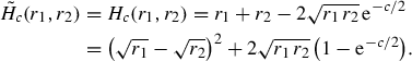 (5.5)
(5.5) -
E.2
For \(p=0\), \(F_i(s)=U_0(s)=s-\log s-1\), and \(R_i(r)=U_1(r)\) we obtain
 (5.6)
(5.6) -
E.3
In the power-like case with \(p\in \mathbb {R}\setminus \{ 0,1\}\) we start from
$$\begin{aligned} F_i(s):=U_p(s)=\frac{1}{p(p{-}1)}\big (s^p-p(s{-}1)-1\big ),\quad R_i(r)=U_{1-p}(r) \end{aligned}$$and obtain, for \(r_1,r_2>0\),
 (5.7)
(5.7)where \(q=p/(p{-}1)\). In fact, we have
$$\begin{aligned}&\theta \big (U_{1-p}(\tfrac{r_1}{\theta })+ U_{1-p}(\tfrac{r_2}{\theta })+c\big )= \frac{r_1^{1-p}+r_2^{1-p}}{p(p{-}1)}\theta ^p\\&\quad \qquad \qquad \qquad \qquad \qquad \qquad \qquad +\frac{1}{p} (r_1{+}r_2)+\frac{1}{p{-}1}((p{-}1)c-2)\theta )\\&\quad =\frac{1}{p} (r_1{+}r_2)+ \frac{1}{p{-}1} \Big [ \frac{1}{p} \Big ((r_1^{1-p}+r_2^{1-p})^{1/p}\,\theta \Big )^p- \big (2-(p{-}1)c\big )\theta \Big ], \end{aligned}$$and (5.7) follows by minimizing w.r.t. \(\theta \). For example, when \(p=q=2\),
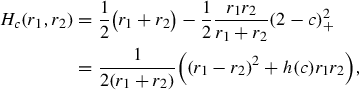 (5.8)
(5.8)where \(h(c)=c(4-c)\) if \(0\le c\le 2\) and 4 if \(c\ge 2\). For \(p=-1\) and \(q=1/2\) equation (5.7) yields
 (5.9)
(5.9) -
E.4
In the case of the total variation entropy \(R_i(s)=V(s)=|s-1|\) we easily find
$$\begin{aligned} {\tilde{H}}_c(r_1,r_2)= & {} H_c(r_1,r_2)=r_1+r_2 -(2-c)_+(r_1\wedge r_2)\\= & {} |r_2-r_1|+(c\wedge 2) (r_1\wedge r_2). \end{aligned}$$


The following dual characterization of \(H_c\) nicely explains the crucial role of \(H_c\).
Lemma 5.3
(Dual characterization of \(H_c\)) For every \(c\ge 0\) the function \(H_c\) admits the dual representation


In particular it is lower semicontinuous, convex and positively 1-homogeneous (thus sublinear) with respect to \((r_1,r_2)\), nondecreasing and concave w.r.t. c, and satisfies

Moreover,
-
(a)
the function \(H_c\) coincides with \({\tilde{H}}_c\) in the interior of its domain; in particular, if \(F_i(0)<\infty \) then \(H_c(r_1,r_2)={\tilde{H}}_c(r_1,r_2)\) whenever \(r_1r_2>0\).
-
(b)
If \({(F_1)'_\infty }+c\ge -{(F_2)_0'}\) and \({(F_2)'_\infty }+c\ge -{(F_1)_0'}\), then
$$\begin{aligned} H_c(r_1,r_2)=\sum _i F_i(0)r_i\quad \text {if }r_1r_2=0. \end{aligned}$$(5.13)
Proof
Since \(\sup {\text {D}}(R^*_i)=F_i(0)\) by (2.33), one immediately gets (5.10) in the case \(c=\infty \); we can thus assume \(c<\infty \).
It is not difficult [23, Chap. IV, Sect. 2.2] to check that the perspective function \((r_1,r_2,\theta )\mapsto \theta \big (R_1(r_1/\theta )+R_2(r_2/\theta )+c\big )\) is jointly convex in \([0,\infty )\times [0,\infty )\times (0,\infty )\) so that \({\tilde{H}}_c\) is a convex and positive 1-homogeneous function. It is also proper (i.e. it is not identically \(+\infty \)) thanks to (3.1), and it is concave w.r.t c since it is the infimum of a family of affine functions in c.
By Legendre duality [41, Thm.12.2], its lower semicontinuous envelope is given by
where
Now, (5.11) immediately follows from (5.10) by the usual change of variable \(\varphi _i=R^*_i(\psi _i)\), recall (2.31) and \(F^{\circ }_i(\varphi _i)=-F^*_i(-\varphi _i)\).
In order to prove point (a) it is sufficient to recall that convex functions are always continuous in the interior of their domain [41, Thm. 10.1]. In particular, since \(\lim _{\theta \downarrow 0} \theta \big (R_1(r_1/\theta ) + R_2(r_2/\theta )+c)= \sum _{i}{(R_i)'_\infty }r_i=\sum _i F_i(0)r_i\) for every \(r_1,r_2>0\), we have \({\tilde{H}}_c(r_1,r_2)\le \sum _i F_i(0)r_i\), so that \({\tilde{H}}_c\) is always finite if \(F_i(0)<\infty \).
Concerning (b), it is obvious when \(r_1=r_2=0\). When \(r_1>r_2=0\), the facts that \(\sup {\text {D}}(R^*_i)=F_i(0)\), \(\lim _{r\uparrow F_i(0)}R^*_i(r) =-{(F_i)_0'}\), and \(\inf R^*_i=-{(F_i)'_\infty }\) (see (2.33)) yield
An analogous formula holds when \(0=r_1<r_2\). \(\square \)
A simple consequence of Lemma 5.3 and (2.31) is the lower bound

We now introduce the integral functional associated with the marginal perspective cost (5.3), which is based on the Lebesgue decomposition \(\mu _i=\varrho _i\gamma _i+\mu _i^\perp \) (see Lemma 2.3),

where we adopted the same notation as in (3.27). Let us first show that \(\mathscr {H}\) is always greater than \(\mathscr {D}\).
Lemma 5.4
For every  ,
,  , \({\varvec{\varphi }}\in {\varvec{\Phi }}\), \(\varrho _i\in \mathrm {L}^1_+(X_i,\gamma _i)\) with \(\mu _i=\varrho _i\gamma _i+\mu _i'\), we have

Proof
Recalling that \(F^{\circ }_i(\varphi _i)=-F^*(-\varphi _i)\le F_i(0)\) by (2.19) and (2.45), and using (5.15) with \(r_j=\rho _j\) and \(\psi _j = F^{\circ }_j(\rho _j)\) we have

\(\square \)
An immediate consequence of the previous lemma is the following important result concerning the marginal perspective cost functional \(\mathscr {H}\) defined by (5.16). It can be nicely compared to the Reverse Entropy-Transport functional \(\mathscr {R}\) for which Theorem 3.11 stated \(\mathscr {R}(\mu _1,\mu _2|{\varvec{\gamma }})=\mathscr {E}({\varvec{\gamma }}|\mu _1,\mu _2)\).
Theorem 5.5
For every  ,
,  and \({\varvec{\varphi }}\in {\varvec{\Phi }}\) we have
In particular

and  if and only if it minimizes \(\mathscr {H}(\mu _1,\mu _2|\cdot )\) in
  and satisfies

where \(\varrho _i\) is defined as in (2.8). If moreover the following conditions
are satisfied, then

Proof
The inequality \(\mathscr {R}(\mu _1,\mu _2|{\varvec{\gamma }})\ge \mathscr {H}(\mu _1,\mu _2|{\varvec{\gamma }})\) is an immediate consequence of the fact that  for every \(r_i,c\in [0,\infty ]\), obtained by choosing \(\theta =1\) in (5.1). The estimate \(\mathscr {H}(\mu _1,\mu _2|{\varvec{\gamma }})\ge \mathscr {D}({\varvec{\varphi }}|\mu _1,\mu _2)\) was shown in Lemma 5.4.
By using the “reverse” formulation of  in terms of the functional \(\mathscr {R}(\mu _1,\mu _2|{\varvec{\gamma }})\) given by Theorem 3.11 and applying Theorem 4.11 we obtain (5.19) and the characterization (5.20).
To establish the identity (5.22) we note that the difference to (5.19) only lies in dropping the additional restriction \(\mu _i^\perp =0\). When both \(F_1(0)=F_2(0)=+\infty \) the equivalence is obvious since the finiteness of the functional \({\varvec{\gamma }}\mapsto \mathscr {H}(\mu _1,\mu _2|{\varvec{\gamma }})\) yields \(\mu _1^\perp =\mu _2^\perp =0\).
In the general case, one immediately see that the right-hand side \(E'\) of (5.22) (with “\(\inf \)” instead of “\(\min \)”) is larger than  , since the infimum of \(\mathscr {H}(\mu _1,\mu _2|\cdot )\) is constrained to the smaller set of plans \({\varvec{\gamma }}\) satisfying \(\mu _i\ll \gamma _i\). On the other hand, if
  with \(\mu _i=\varrho _i{\bar{\gamma }}_i+\mu _i^\perp \) and \({\tilde{m}}_i:=\mu _i^\perp (X_i)>0\), we can consider \({\varvec{\gamma }}:= {\bar{{\varvec{\gamma }}}}+ \frac{1}{{\tilde{m}}_1{\tilde{m}}_2}\mu _1^\perp \otimes \mu _2^\perp \) which satisfies \(\mu _i\ll \gamma _i\); by exploiting the fact that
  by (5.12), we obtain

so that we have  . The case when only one (say \(\mu _2^\perp \)) of the measures \(\mu _i^\perp \) vanishes can be treated in the same way: since in this case \({\tilde{m}}_1=\mu _1^\perp (X_1)>0\) and therefore \(F_1(0)<\infty \), by applying (5.21) we can choose \({\varvec{\gamma }}:= {\bar{{\varvec{\gamma }}}}+ \frac{1}{{\tilde{m}}_1}\mu _1^\perp \otimes \delta _{{\bar{x}}_2}\), obtaining

\(\square \)
Remark 5.6
Notice that (5.21) is always satisfied if the spaces \(X_i\) are uncountable. If \(X_i\) is countable, one can always add an isolated point \({\bar{x}}_i\) (sometimes called “cemetery”) to \(X_i\) and consider the augmented space \({\bar{X}}_i=X_i\sqcup \{{\bar{x}}_i\}\) obtained as the disjoint union of X and \({\bar{x}}_i\), with augmented cost \({\bar{\mathsf{c}}}\) which extends \(\mathsf{c}\) to \(+\infty \) on \({\bar{X}}_1\times {\bar{X}}_2\setminus (X_1\times X_2)\). We can recover (5.22) by allowing \({\varvec{\gamma }}\) in  .
.
5.2 Entropy-transport problems with “homogeneous” marginal constraints
In this section we will exploit the 1-homogeneity of the marginal perspective function \(\mathscr {H}\) in order to derive a last representation of the functional  , related to the new notion of homogeneous marginals. We will confine our presentation to the basic facts, and we will devote the second part of the paper to develop a full theory for the specific case of the Logarithmic Entropy-transport case.
In particular, the following construction (typical in the Young measure approach to variational problems) allows us to consider the entropy-transport problems in a setting of greater generality. We replace a pair \((\gamma ,\varrho )\), where \(\gamma \) and \(\varrho \) are a measure on X and a nonnegative Borel function, by a measure  on the extended space \(Y = X\times [0,\infty )\). The original pair \((\gamma ,\varrho )\) corresponds to a measure \(\alpha =(x,\varrho (x))_\sharp \gamma \) concentrated on the graph of \(\varrho \) in Y and whose first marginal is \(\gamma \).
Homogeneous marginals. In the usual setting of Sect. 3.1, we consider the product spaces \(Y_i:=X_i\times [0,\infty )\) endowed with the product topology and denote the generic points in \(Y_i\) with \(y_i=(x_i,r_i)\), \(x_i\in X_i \) and \( r_i\in [0,\infty )\) for \(i=1,2\). Projections from \({\varvec{Y}}:=Y_1\times Y_2\) onto the various coordinates will be denoted by \(\pi ^{y_i},\ \pi ^{x_i},\ \pi ^{r_i}\) with obvious meaning.
For \(p>0\) and \({\varvec{y}}\in {\varvec{Y}}\) we will set \(|{\varvec{y}}|_p^p:=\sum _i |r_i|^p\) and call \(\mathcal {M}_{p} ({\varvec{Y}})\) (resp.  ) the space of measures
  (resp.
  ) such that
If \({\varvec{\alpha }}\in \mathcal {M}_{p}({\varvec{Y}})\) the measures \(r_i^p{\varvec{\alpha }}\) belong to  , which allow us to define the “p-homogeneous” marginal
  of \({\varvec{\alpha }}\in \mathcal {M}_{p} ({\varvec{Y}})\) as the \(x_i\)-marginal of \(r_i^p {\varvec{\alpha }}\), namely

The maps  are linear and invariant with respect to dilations: if \(\vartheta :{\varvec{Y}}\rightarrow (0,\infty )\) is a Borel map in \(\mathrm {L}^p({\varvec{Y}},{\varvec{\alpha }})\) and \(\mathrm {prd}_\vartheta ({\varvec{y}}):=(x_1,r_1/\vartheta ({\varvec{y}});x_2,r_2/\vartheta ({\varvec{y}}) )\), we set
Using (5.24) we obviously have

In particular, for \({\varvec{\alpha }}\in \mathcal {M}_{p} ({\varvec{Y}})\) with \({\varvec{\alpha }}({\varvec{Y}})>0\), by choosing
we obtain a rescaled probability measure \({\tilde{{\varvec{\alpha }}}}\) with the same homogeneous marginals as \({\varvec{\alpha }}\) and concentrated on  :
:

Entropy-transport problems with prescribed homogeneous marginals. Given  we now introduce the convex sets

Clearly  and they are nonempty since every plan of the form
belongs to  . It is not difficult to check that
  is also narrowly closed, while, on the contrary, this property fails for
  if \(\mu _1(X_1)\mu _2(X_2)\ne 0\). To see this, it is sufficient to consider any
  and look at the vanishing sequence \({\mathrm {dil}}_{n^{-1},p}({\varvec{\alpha }})\) for \(n\rightarrow \infty \).
There is a natural correspondence between  (resp.
  ) and
) and  (resp.
  ) induced by the map \({\varvec{Y}}\ni (x_1,r_1;x_2,r_2)\mapsto (x_1,r_1^p;x_2,r_2^p).\) For plans
  we can prove a result similar to Lemma 5.4 but now we obtain a linear functional in \({\varvec{\alpha }}\).
Lemma 5.7
For \(p\in (0,\infty )\),  , \({\varvec{\varphi }}\in {\varvec{\Phi }}\), and
  we have

Proof
The calculations are quite similar to the proof of Lemma 5.4:

\(\square \)
As a consequence, we can characterize the entropy-transport minimum via measures  .
.
Theorem 5.8
For every  , \(p\in (0,\infty )\) we have


Moreover, for every plan  (resp. optimal for (5.19) or for (5.22)) with \(\mu _i=\varrho _i\gamma _i+\mu _i^\perp \), the plan \({\varvec{\alpha }}:=(x_1,\varrho _1^{1/p}(x_1);x_2,\varrho _2^{1/p}(x_2))_\sharp {\varvec{\gamma }}\) realizes the minimum of (5.31) (resp. (5.32) or (5.33)).
Remark 5.9
When \(F_i(0)=+\infty \) (5.31) and (5.32) simply read as

\(\square \)
Proof of Theorem 5.8
Let us denote by \(E'\) (resp. \(E''\), \(E'''\)) the right-hand side of (5.31) (resp. of (5.32), (5.33)), where “\(\min \)” has been replaced by “\(\inf \)”. If  and \(\mu _i=\varrho _i\gamma _i+\mu _i^\perp \) (in the case of (5.33) \(\mu _i^\perp =0\)) is the usual Lebesgue decomposition as in Lemma 2.3 , we can consider the plan \({\varvec{\alpha }}:=(x_1,\varrho _1^{1/p}(x_1);x_2,\varrho _2^{1/p}(x_2))_\sharp {\varvec{\gamma }}\).
Since the map \((\varrho _1^{1/p},\varrho _2^{1/p}):{\varvec{X}}\rightarrow \mathbb {R}^2\) is Borel and takes values in a metrizable and separable space, it is Lusin \({\varvec{\gamma }}\)-measurable [44, Thm 5, p. 26], so that \({\varvec{\alpha }}\) is a Radon measure in  . For every nonnegative \(\phi _i\in \mathrm {B}_b(X_i)\) we easily get
so that  ,
,  , and
, and

Taking the infimum w.r.t. \({\varvec{\gamma }}\) and recalling (3.30) we get  . Since
  it is also clear that \(E'\ge E''\).
On the other hand, Lemma 5.7 shows that \(E''\ge \mathscr {D}({\varvec{\varphi }}|\mu _1,\mu _2)\) for every \({\varvec{\varphi }}\in {\varvec{\Phi }}\). Applying Theorem 4.11 we get  .
.
Concerning \(E'''\) it is clear that  . When (5.21) hold, by choosing \({\varvec{\alpha }}\) induced by a minimizer of (5.22) we get the opposite inequality
  .
.
If (5.21) does not hold, we can still apply a slight modification of the argument at the end of the proof of Theorem 5.5. The only case to consider is when only one of the two measures \(\mu _i^\perp \) vanishes: just to fix the ideas, let us suppose that \({\tilde{m}}_1=\mu _1^\perp (X_1)>0=\mu _2^\perp (X_2)\). If  and \({\bar{{\varvec{\alpha }}}}\) is obtained as above, we can just set \({\varvec{\alpha }}:={\bar{{\varvec{\alpha }}}}+(\mu _1^\perp \times \delta _1)\times (\nu \times \delta _0)\) for an arbitrary
  . It is clear that
  and
and

which yields  .
.
Remark 5.10
(Rescaling invariance) By recalling (5.27a,b) and exploiting the 1-homogeneity of H it is not restrictive to solve the minimum problem (5.32) in the smaller class of probability plans concentrated in

First, we note that it is not restrictive to assume that \({\varvec{\alpha }}(\{{\varvec{y}}\in {\varvec{Y}}:|{\varvec{y}}|_{ p }=0\})=0\) in (5.32): we can always replace \({\varvec{\alpha }}\) with  since \(H(x_1,0;x_2,0)=0\) for every \(x_i\in X_i\) and the homogeneous marginals of \({\varvec{\alpha }}\) and \({\varvec{\alpha }}'\) coincide. As a second step, for every
  with \({\varvec{\alpha }}({\varvec{Y}})>0\), the choice \({\tilde{{\varvec{\alpha }}}}\) given by (5.27a,b) yields a new probability plan concentrated on
  with the same homogeneous marginals as \({\varvec{\alpha }}\) and satisfying

where \(\vartheta \) is the function defined in (5.27a) and we used the 1-homogeneity of H w.r.t. the variables \((r_1,r_2)\).
Part II. The Logarithmic Entropy-Transport problem and the Hellinger–Kantorovich distance
6 The Logarithmic Entropy-Transport (LET) problem
Starting from this section we will study a particular Entropy-Transport problem, whose structure reveals surprising properties.
6.1 The metric setting for Logarithmic Entropy-Transport problems
Let \((X,\tau )\) be a Hausdorff topological space endowed with an extended distance function \(\mathsf{d}:X\times X\rightarrow [0,\infty ]\) which is lower semicontinuous w.r.t. \(\tau \); we refer to \((X,\tau ,\mathsf{d})\) as an extended metric-topological space. In the most common situations, \(\mathsf{d}\) will take finite values, \((X,\mathsf{d})\) will be separable and complete and \(\tau \) will be the topology induced by \(\mathsf{d}\); nevertheless, there are interesting applications where nonseparable extended distances play an important role, so that it will be useful to deal with an auxiliary topology, see e.g. [1, 3].
From now on we suppose that \(X_1=X_2=X\). We choose the logarithmic entropies
and a cost \(\mathsf{c}\) depending on the distance \(\mathsf{d}\) through the function \(\ell :[0,\infty ]\rightarrow [0,\infty ]\) via
so that
Let us collect a few key properties that will be relevant in the sequel.
-
LE.1
\(F_i\) are superlinear, \(\mathrm {C}^\infty \) in \((0,\infty )\), strictly convex, with \({\text {D}}(F_i)=[0,\infty )\), \(F_i(0)=1\), and \({(F_i)_0'}=-\infty \). For \(s>0\) we have \(\partial F_i(s)=\{\log s\}\).
-
LE.2
\(R_i(r)=rF_i(1/r)=r-1-\log r\), \(R_i(0)=+\infty \), \({(R_i)'_\infty }=1\).
-
LE.3
\(F^*_i(\phi )=\exp (\phi )-1\), \(F^{\circ }_i(\varphi )=1-\exp (-\varphi )\), \({\text {D}}(F^*_i)={\text {D}}(F^{\circ }_i)=\mathbb {R}\).
-
LE.4
\(R^*_i(\psi )=-\log (1-\psi )\) for \(\psi <1\) and \(R^*_i(\psi )=+\infty \) for \(\psi \ge 1\).
-
LE.5
The function \(\ell \) can be characterized as the unique solution of the differential equation
$$\begin{aligned} \ell ''(d)=2\exp (\ell (d)),\quad \ell (0)=\ell '(0)=0,\quad \end{aligned}$$(6.4)since it satisfies
$$\begin{aligned} \ell (d)=-\log \big ({\cos ^2(d)}\big )= 2\int _0^d \tan (s)\,\mathrm {d}s, \quad d\in [0,\pi /2), \end{aligned}$$(6.5)so that
$$\begin{aligned}&\ell (d)\ge d^2,\quad \ell '(d)=2\tan d\ge 2d,\quad \ell ''(d)\ge 2. \end{aligned}$$(6.6)In particular \(\ell \) is strictly increasing and uniformly 2-convex. It is not difficult to check that \(\sqrt{\ell }\) is also convex: this property is equivalent to \(2\ell \ell ''\ge (\ell ')^2\) and a direct calculation shows
$$\begin{aligned} 2\ell \ell ''-(\ell ')^2=4\log (1+\tan ^2(d))(1+\tan ^2(d))-4\tan ^2(d)\ge 0 \end{aligned}$$since \((1+r)\log (1+r)\ge r\).
-
LE.6
 for \(c<\infty \), so that
  (6.7)
(6.7)where we set
$$\begin{aligned} \mathsf{d}_a(x_1,x_2):=\mathsf{d}(x_1,x_2)\wedge a \quad \text { for } x_i\in X,\ a\ge 0. \end{aligned}$$(6.8)Since the function
 (6.9)
(6.9)will have an important geometric interpretation (see Sect. 7.1), in the following we will choose the exponent \(p=2\) in the setting of Sect. 5.2.
 for
for 

We keep the usual notation \({\varvec{X}}=X\times X\), identifying \(X_1\) and \(X_2\) with X and letting the index i run between 1 and 2, e.g. for  the marginals are denoted by \(\gamma _i=(\pi ^i)_\sharp {\varvec{\gamma }}\).
Problem 6.1
(The Logarithmic Entropy-Transport problem) Let \((X,\tau ,\mathsf{d})\) be an extended metric-topological space, \(\ell \) and \(\mathsf{c}\) be as in (6.2). Given  find
find  minimizing

where \(\sigma _i=\frac{\mathrm {d}\gamma _i}{\mathrm {d}\mu _i}\). We denote by  the set of all the minimizers \({\varvec{\gamma }}\) in (6.10).
6.2 The Logarithmic Entropy-Transport problem: main results
In the next theorem we collect the main properties of the Logarithmic Entropy-Transport (LET) problem relying on the reverse function \(\mathscr {R}\) from Sect. 3.5, cf. (3.28), and \(\mathscr {H}\) from Sect. 5.1, cf. (5.16).
Theorem 6.2
(Direct formulation of the LET problem) Let  be given and let \(\ell ,\mathsf{d}_{\pi /2}\) be defined as in (6.2) and (6.8).
- (a) :
-
Existence of optimal plans. There exists an optimal plan
 solving Problem 6.1. The set
  is convex and compact in
  ,
,  is a convex and positively 1-homogeneous functional (see (4.41)) satisfying
  .
. - (b) :
-
Reverse formulation
 . The functional
  has the equivalent reverse formulation as
where
 (6.11)
and \({\bar{{\varvec{\gamma }}}}\) is an optimal plan in
 if and only if it minimizes (6.11).
 - (c) :
-
The homogeneous perspective formulation
 . The functional
  can be equivalently characterized as
  (6.12)
and \(\gamma _i=\varrho _i\mu _i+\mu _i^\perp \). Moreover, every plan
 provides a solution to (6.12).
 solving Problem
  is convex and compact in
  ,
,  is a convex and positively 1-homogeneous functional (see (
 .
. . The functional
  has the equivalent reverse formulation as

 if and only if it minimizes (
 . The functional
  can be equivalently characterized as
 provides a solution to (
Proof
The variational problem (6.10) fits in the class considered by Problem 3.1, in the basic coercive setting of Sect. 3.1 since the logarithmic entropy (6.1) is superlinear with domain \([0,\infty )\). The problem is always feasible since \(U_1(0)=1\) so that (3.6) holds.
-
(a)
follows by Theorem 3.3(i); the upper bound of
 is a particular case of (3.7), and its convexity and 1-homogeneity follows by Corollary 4.13.
 -
(b)
is a consequence of Theorem 3.11.
- (c)
 is a particular case of (
We consider now the dual representation of  ; recall that \(\mathrm {LSC}_s(X)\) denotes the space of simple (i.e. taking a finite number of values) lower semicontinuous functions and for a pair \(\phi _i:X\rightarrow \mathbb {R}\) the symbol \(\phi _1\oplus \phi _2\) denotes the function \((x_1,x_2)\mapsto \phi _1(x_1)+\phi _2(x_2)\) defined in \({\varvec{X}}\). In part a) we relate to Sect. 4.2, whereas b)–d) discusses the optimality conditions from Sect. 4.4.
Theorem 6.3
(Dual formulation and optimality conditions)
(a) The dual problem  . For all
  we have


where  . The same identities hold if the space \(\mathrm {LSC}_s(X)\) is replaced by \(\mathrm {LSC}_b(X)\) or \(\mathrm {B}_b(X)\) in (6.13) and (6.14). When the topology \(\tau \) is completely regular (in particular when \(\mathsf{d}\) is a distance and \(\tau \) is induced by \(\mathsf{d}\)) the space \(\mathrm {LSC}_s(X)\) can be replaced by \(\mathrm {C}_b(X)\) as well.
(b) Optimality conditions. Let us assume that \(\mathsf{d}\) is continuous. A plan  is optimal if and only if its marginals \(\gamma _i\) are absolutely continuous w.r.t. \(\mu _i\),
and there exist Borel sets \(A_i\subset \mathop {\mathrm{supp}}\nolimits \gamma _i\) with \(\gamma _i(X\setminus A_i)=0\) and Borel densities \(\sigma _i:A_i\rightarrow (0,\infty )\) of \(\gamma _i\) w.r.t. \(\mu _i\) such that
or, equivalently, in terms of the densities \(\varrho _i=\sigma _i^{-1}\) of \(\mu _i\) w.r.t. \(\gamma _i\)
(c) \(\ell (\mathsf{d})\) -cyclical monotonicity. Every optimal plan  is a solution of the optimal transport problem \(\mathsf{T}\) with cost \(\ell (\mathsf{d})\) (see (3.15) of Sect. 3.3) between its marginals \(\gamma _i\). In particular it is \(\ell (\mathsf{d})\)-cyclically monotone, i.e. it is concentrated on a Borel set \(G\subset {\varvec{X}}\) (\(G=\mathop {\mathrm{supp}}\nolimits ({\varvec{\gamma }})\) when \(\mathsf{d}\) is continuous) such that for every choice of \((x_1^n,x_2^n)_{n=1}^N\subset G\) and every permutation \(\kappa :\{1,\ldots ,N\}\rightarrow \{1,\ldots ,N\}\)
(d) Generalized potentials. If \({\varvec{\gamma }}\) is optimal and \(A_i\), \(\sigma _i\) are defined as in b) above, the Borel potentials \(\varphi _i,\psi _i:X\rightarrow {\bar{\mathbb {R}}}\)
satisfy \(\varphi _1\oplus _o\varphi _2\le \ell (\mathsf{d})\), \(\log (1{-}\psi _1)\oplus _o\log (1{-}\psi _2)\ge \ell (\mathsf{d})\), and the optimality conditions corresponding to (4.50)
Moreover \(\mathrm {e}^{-\varphi _i},\psi _i\in \mathrm {L}^1(X,\mu _i)\) and

Proof
Identity (6.13) follows by Theorem 4.11, recalling the definition (4.11) of \({\varvec{\Phi }}\) and the fact that \(F^{\circ }_i(\varphi )=1-\exp (-\varphi )\).
Identity (6.14) follows from Proposition 4.3 and the fact that \(R^*_i(\psi )=-\log (1-\psi )\). Notice that the definition (4.7) of \({\varvec{\Psi }}\) ensures that we can restrict the supremum in (6.14) to functions \(\psi _i\) with \(\sup _X \psi _i<1\). We have discussed the possibility to replace \(\mathrm {LSC}_s(X)\) with \(\mathrm {LSC}_b(X)\), \(\mathrm {B}_b(X)\) or \(\mathrm {C}_b(X)\) in Corollary 4.12.
The statement of point (b) follows by Corollary 4.18; notice that the  problem is always feasible.
Point (c) is an obvious consequence of the optimality of \({\varvec{\gamma }}\).
Point (d) can be easily deduced by (b) or by applying Corollaries 4.17 and 4.18, observing that the formula defining \(\varphi _i\) of (6.21) corresponds to (4.48) with \({(F_i)'_\infty }=+\infty =-{(F_i)_0'}\) and the optimality condition corresponds to (4.50). Finally, \(\psi _i\) are just related to \(\varphi _i\) by \(\psi _i=F^{\circ }_i(\varphi _i)=1-\exp (-\varphi _i)\). \(\square \)
In the one-dimensional case, the \(\ell (\mathsf{d})\)-cyclic monotonicity of part (c) of the previous theorem reduces to classical monotonicity.
Corollary 6.4
(Monotonicity of optimal plans in \(\mathbb {R}\)) When \(X=\mathbb {R}\) with the usual distance, the support of every optimal plan \({\varvec{\gamma }}\) is a monotone set, i.e.
Proof
As the function \(\ell \) is uniformly convex, (6.20) is equivalent to monotonicity. \(\square \)
The next result provides a variant of the reverse formulation in Theorem 6.2, which expresses the  problem as a supremum of the linear mass functional on \({\varvec{\gamma }}\) on a convex set characterized by the marginals of \({\varvec{\gamma }}\) and the cost.
Corollary 6.5
For all  we have

Proof
Let us denote by \(M'\) the right-hand side and let  be a plan satisfying the conditions of (6.24). If \(A_i\) are Borel sets with \(\gamma _i(X\setminus A_i)=0\) and \(\sigma _i:X\rightarrow (0,\infty )\) are Borel densities of \(\gamma _i\) w.r.t. \(\mu _i\), the densities \(\varrho _i\) of \(\mu _i\) w.r.t. \(\gamma _i\) satisfy \(\varrho _i(x_i)=1/\sigma _i(x_i)\) in \(A_i\) so that \(\sigma _1(x_1)\sigma _2(x_2)\le \cos ^2(\mathsf{d}_{\pi /2}(x_1,x_2))\) yields \(\varrho _1(x_1)\varrho _2(x_2)\cos ^2(\mathsf{d}_{\pi /2}(x_1,x_2))\ge 1\). Since \((\log \varrho _i)_+\in \mathrm {L}^1(X,\gamma _i)\) we have
By (6.11) we get  . On the other hand, choosing any
  the optimality condition (6.17) shows that \({\bar{{\varvec{\gamma }}}}\) is an admissible competitor for (6.24) and (6.22) shows that
  . \(\square \)
Combining (6.12), (6.13), (6.14), and (6.24), we find that the nonnegative and concave functional  can be represented as in the following equivalent ways:


The next result concerns uniqueness of the optimal plan \({\varvec{\gamma }}\) in the Euclidean case \(X=\mathbb {R}^d\). We will use the notion of approximate differential (denoted by \({\tilde{\mathrm {D}}}\)), see e.g. [2, Def. 5.5.1].
Theorem 6.6
(Uniqueness) Let  and
and  .
.
-
(i)
The marginals \(\gamma _i=\pi ^i_\sharp {\varvec{\gamma }}\) are uniquely determined.
-
(ii)
If \(X=\mathbb {R}\) with the usual distance then \({\varvec{\gamma }}\) is the unique element of
 .
. -
(iii)
If \(X=\mathbb {R}^d\) with the usual distance, \(\mu _1\ll {\mathscr {L}}^{d}\) is absolutely continuous, and \(A_i\subset \mathbb {R}^d\) and \(\sigma _i:A_i\rightarrow (0,\infty )\) are as in Theorem 6.3 b), then \(\sigma _1\) is approximately differentiable at \(\mu _1\)-a.e. point of \(A_1\) and \({\varvec{\gamma }}\) is the unique element of
 . The transport plan \({\varvec{\gamma }}\) is concentrated on the graph of a function \({\varvec{t}}:\mathbb {R}^d\rightarrow \mathbb {R}^d\) satisfying $$\begin{aligned} {\varvec{t}}(x_1)= & {} x_1- \frac{\arctan (|{\varvec{\xi }}(x_1)|)}{|{\varvec{\xi }}(x_1)|} {\varvec{\xi }}(x_1),\nonumber \\ {\varvec{\xi }}(x_1)= & {} -\frac{1}{2}{\tilde{\mathrm {D}}}\log \sigma _1(x_1) \end{aligned}$$(6.29)
 .
. . The transport plan
 Proof
(i) follows directly from Lemma 3.5.
(ii) follows by Theorem 6.3(c), since whenever the marginals \(\gamma _i\) are fixed there is only one plan with monotone support in \(\mathbb {R}\) (see e.g. [42, Chap. 2]).
In order to prove (iii) we adapt the argument of [2, Thm. 6.2.4] to our singular setting, where the cost \(\mathsf{c}\) can take the value \(+\infty \).
Let \(A_i\subset \mathbb {R}^d\) and \(\sigma _i:A_i\rightarrow (0,\infty )\) as in Theorem 6.3 b); notice that since \(\sigma _1>0\) in \(A_1\) the classes of \(\mu _1\)- and \(\gamma _1\)-negligible subsets of \(A_1\) coincide. Since \(\mu _1=u{\mathscr {L}}^{d}\ll {\mathscr {L}}^{d}\) with density \(u \in L^1(\mathbb {R}^d)\), up to removing a \(\mu _1\)-negligible set (and thus \(\gamma _1\)-negligible) from \(A_1\), it is not restrictive to assume that \(u(x_1)>0\) everywhere in \(A_1\), so that the classes of \({\mathscr {L}}^{d}\)- and \(\mu _1\)-negligible subsets of \(A_1\) coincide. For every \(n\in \mathbb {N}\) we define
The functions \(s_n\) are bounded and Lipschitz in \(\mathbb {R}^d\) and therefore differentiable \({\mathscr {L}}^{d}\)-a.e. by Rademacher’s Theorem. Since \(\mu _1\) is absolutely continuous w.r.t. \({\mathscr {L}}^{d}\) we deduce that \(s_n\) are differentiable \(\mu _1\)-a.e. in \(A_1\).
By (6.16) we have \(\sigma _1(x_1)\ge s_n(x_1)\) in \(A_1\). By (6.17) we know that for \(\gamma _1\)-a.e. \(x_1\in A_1\) there exists \(x_2\in A_2\) such that \(|x_1-x_2|<\pi /2\) and \(\sigma _1(x_1)=\cos ^2(|x_1-x_2|)/\sigma _2(x_2)\) so that \(\sigma _1(x_1)=s_n(x_1)\) for n sufficiently big and hence the family \((B_n)_{n\in \mathbb {N}}\) of sets \(B_n:=\{x_1\in A_1:\sigma _1(x_1)>s_n(x_1)\}\) is decreasing (since \(s_n\) is increasing and dominated by \(\sigma _1\)) and has \({\mathscr {L}}^{d}\)-negligible intersection.
It follows that \(\gamma _1\)-a.e. \(x_1\in A_1\) is a point of \({\mathscr {L}}^{d}\)-density 1 of \(\{x_1\in A_1:\sigma _1(x_1)=s_n(x_1)\}\) for some \(n\in \mathbb {N}\) and \(s_n\) is differentiable at \(x_1\). Let us denote by \(A_1'\) the set of all \(x_1\in A_1\) such that \(\sigma _1\) is approximately differentiable at every \(x_1\in A_1'\) with approximate differential \({\tilde{\mathrm {D}}}\sigma _1(x_1)\) equal to \(\mathrm {D}s_n(x_1)\) for n sufficiently big.
Suppose now that \(x_1\in A_1'\) and \(\sigma _1(x_1)=\cos ^2(|x_1-x_2|)/\sigma _2(x_2)\) for some \(x_2\in A_2\). Since by (6.16) and (6.17) the map \(x_1'\mapsto \cos ^2(|x_1'-x_2|)/\sigma _1(x_1')\) attains its maximum at \(x_1'=x_1\), we deduce that
so that \(x_2\) is uniquely determined, and (6.29) follows. \(\square \)
We conclude this section with the last representation formula for  given in terms of transport plans \({\varvec{\alpha }}\) in \({\varvec{Y}}:=Y\times Y\) with \(Y:=X\times [0,\infty )\) with constraints on the homogeneous marginals, keeping the notation of Sect. 5.2. Even if it seems the most complicated one, it will provide the natural point of view in order to study the metric properties of the
  functional, and it will play a crucial role in Sect. 7.6, where the link between the
  formulation and the Hellinger–Kantorovich distance will be studied. The interest of (6.34) relies in the particular form of its integrand, by recalling that by (5.4) and (6.9) we have

Theorem 6.7
For every  we have


Moreover, for every plan  and every pair of Borel densities \(\varrho _i\) as in (6.11) the plan \({\bar{{\varvec{\alpha }}}}:=(x_1,\sqrt{\varrho _1(x_1)};x_2,\sqrt{\varrho _2(x_2)})_\sharp {\bar{{\varvec{\gamma }}}}\) is optimal for (6.33) and (6.32).
Proof
Identity (6.33) (resp. (6.34)) follows directly by (5.32) (resp. (5.33)) of Theorem 5.8. Relation (6.32) is just a different form for (6.33). \(\square \)
7 The metric side of the LET-functional: the Hellinger–Kantorovich distance
In this section we want to show that the functional

defines a distance in  , which is then called the Hellinger–Kantorovich distance and denoted
  .
.
In order to introduce this distance we will adopt a geometric point of view, which is strictly related to the characterization given in Theorem 6.7: it will mainly exploit the link with Optimal Transport in the so-called geometric cone \(\mathfrak {C}\) constructed on X, cf. [10, Sect. 3.6]. This is possible since the function
appearing in (6.31) and (6.34) with \(a=\pi /2\), is a (possibly extended) squared semidistance in \(Y=X\times [0,\infty )\), whenever \(a\in (0,\pi ]\).
In the next two sections we will briefly study this function and the associated metric for the particular choices of \(a=\pi \) (the canonical one in metric geometry) and \(a=\pi /2\) (related to the minimal cost between a pair of Dirac masses (6.31)): the role of these two values will be clarified in Remark 7.2 and in Sect. 7.6, we also refer to [30, Sect. 3] for more motivation and examples. The induced metric space \(\mathfrak {C}\), can be obtained by taking the quotient with respect to the equivalence classes of points with distance 0. Radon measures on \(\mathfrak {C}\) can be projected to Radon measures on X by taking suitable homogeneous marginals, which will be studied in Sect. 7.2.
The definition and the basic properties of the Hellinger–Kantorovich distance will be given in Sect. 7.3; the main metric properties will be derived in Sects. 7.4 and 7.5: they rely on a refined gluing technique and on the flexibility of the notion of homogeneous marginals, which allow us to transfer many useful properties of the Kantorovich–Wasserstein distance on the cone \(\mathfrak {C}\) to corresponding properties for  . Section 7.6 will then show the equivalent characterization of
  in terms of the Logarithmic Entropy Transport problem
  and its dual formulation, thus providing a direct and robust formulation of
  as a convex minimization problem enjoying all the properties we recalled in the previous section.
7.1 The cone construction
Let us quickly recall a few basic facts concerning the cone construction, referring to [10, Sect. 3.6] for further details. In the extended metric-topological space \((X,\tau ,\mathsf{d})\) of Sect. 6.1, we will denote by \(\mathsf{d}_a:=\mathsf{d}\wedge a\) the truncated distance and by \(y=(x,r)\), \(x\in X,\ r\in [0,\infty )\), the generic points of \(Y:=X\times [0,\infty )\).
It is not difficult to show that the function \(\mathsf{d}_\mathfrak {C}:Y\times Y\rightarrow [0,\infty )\)
is nonnegative, symmetric, and satisfies the triangle inequality (see e.g. [10, Prop. 3.6.13]). We also notice that
which implies the useful estimates
From this it follows that \(\mathsf{d}_\mathfrak {C}\) induces a true distance in the quotient space \(\mathfrak {C}=Y/\sim \) where
Equivalence classes are usually denoted by \(\mathfrak {y}=[y]=[x,r]\), where the vertex [x, 0] plays a distinguished role. It is denoted by \(\mathfrak {o}\), its complement is the open set \(\mathfrak {C}_\mathfrak {o}=\mathfrak {C}\setminus \{\mathfrak {o}\}.\) On \(\mathfrak {C}\) we introduce a topology \(\tau _\mathfrak {C}\), which is in general weaker than the canonical quotient topology: \(\tau _\mathfrak {C}\) neighborhoods of points in \(\mathfrak {C}_\mathfrak {o}\) coincide with neighborhoods in \(Y\), whereas the sets
provide a system of open neighborhoods of \(\mathfrak {o}\). \(\tau _\mathfrak {C}\) coincides with the quotient topology when X is compact.
It is easy to check that \((\mathfrak {C},\tau _\mathfrak {C})\) is a Hausdorff topological space and \(\mathsf{d}_\mathfrak {C}\) is \(\tau _\mathfrak {C}\)-lower semicontinuous. If \(\tau \) is induced by \(\mathsf{d}\) then \(\tau _\mathfrak {C}\) is induced by \(\mathsf{d}_\mathfrak {C}\). If \((X,\mathsf{d})\) is complete (resp. separable), then \((\mathfrak {C}, \mathsf{d}_\mathfrak {C})\) is also complete (resp. separable).
Perhaps the simplest example is provided by the unit sphere \(X=\mathbb {S}^{d-1}=\{x\in \mathbb {R}^d:|x|=1\}\) in \(\mathbb {R}^d\) endowed with the intrinsic Riemannian distance: the corresponding cone \(\mathfrak {C}\) is precisely \(\mathbb {R}^d\).
We denote the canonical projection by
Clearly \(\mathfrak {p}\) is continuous and is an homeomorphism between \(Y\setminus (X\times \{0\})\) and \(\mathfrak {C}_\mathfrak {o}\). A right inverse \(\mathsf{y}:\mathfrak {C}\rightarrow Y\) of the map \(\mathfrak {p}\) can be obtained by fixing a point \(\bar{x}\in X\) and defining
Notice that \(\mathsf {r}\) is continuous and \(\mathsf{x}\) is continuous restricted to \(\mathfrak {C}_\mathfrak {o}\).
A continuous rescaling product from \( \mathfrak {C}\times [0,\infty )\) to \(\mathfrak {C}\) can be defined by

We conclude this introductory section by a characterization of compact sets in \((\mathfrak {C},\tau _\mathfrak {C})\).
Lemma 7.1
(Compact sets in \(\mathfrak {C}\)) A closed set K of \(\mathfrak {C}\) is compact if and only if there is \(r_0>0\) such that its upper sections
are empty for \(\rho >r_0\) and compact in X for \(0<\rho \le r_0\).
Proof
It is easy to check that the condition is necessary.
In order to show the sufficiency, let \(\rho =\inf _K \mathsf {r}\). If \(\rho >0\) then K is compact since it is a closed subset of the compact set \(\mathfrak {p}\big (K(\rho )\times [\rho ,r_0]\big )\).
If \(\rho =0\) then \(\mathfrak {o}\) is an accumulation point of K by (7.7) and therefore \(\mathfrak {o}\in K\) since K is closed. If \(\mathscr {U}\) is an open covering of K, we can pick \(U_0\in \mathscr {U}\) such that \(\mathfrak {o}\in U_{0}\). By (7.7) there exists \(\varepsilon >0\) such that \(K\setminus U_{0}\subset \mathfrak {p}\big (K(\varepsilon )\times [\varepsilon ,r_0]\big )\): since \(\mathfrak {p}\big (K(\varepsilon )\times [\varepsilon ,r_0]\big )\) is compact, we can thus find a finite subcover \(\{U_1,\cdots , U_N\}\subset \mathscr {U}\) of \(K{\setminus } U_{0}\). \(\{U_n\}_{n=0}^N\) is therefore a finite subcover of K. \(\square \)
Remark 7.2
(Two different truncations) Notice that in the constitutive formula defining \(\mathsf{d}_\mathfrak {C}\) we used the truncated distance \(\mathsf{d}_\pi \) with upper threshold \(\pi \), whereas in Theorem 6.7 an analogous formula with \(\mathsf{d}_{\pi /2}\) and threshold \(\pi /2\) played a crucial role. We could then consider the distance
on \(\mathfrak {C}\), which satisfies
The notation (7.11a) is justified by the fact that \(\mathsf{d}_{\pi /2,\mathfrak {C}}\) is still a cone distance associated to the metric space \((X,\mathsf{d}_{\pi /2})\), since obviously \((\mathsf{d}_{\pi /2})_\pi =(\mathsf{d}_{\pi /2})\wedge {\pi /2}=\mathsf{d}_{\pi /2}\). From the geometric point of view, the choice of \(\mathsf{d}_\mathfrak {C}\) is natural, since it preserves important metric properties concerning geodesics (see [10, Thm. 3.6.17] and the next Sect. 8.1) and curvature (see [10, Sect. 4.7] and the next Sect. 8.3).
On the other hand, the choice of \(\mathsf{d}_{\pi /2}\) is crucial for its link with the function \(H\) of (6.9), with Entropy-Transport problems, and with a representation property for the Hopf–Lax formula that we will see in the next sections. Notice that the 1-homogeneous formula (6.7) would not be convex in \((r_1,r_2)\) if one uses \(\mathsf{d}_\pi \) instead of \(\mathsf{d}_{\pi /2}\). Nevertheless, we will prove in Sect. 7.3 the remarkable fact that both \(\mathsf{d}_\pi \) and \(\mathsf{d}_{\pi /2}\) will lead to the same distance between positive measures.
7.2 Radon measures in the cone \(\mathfrak {C}\) and homogeneous marginals
It is clear that any measure  can be lifted to a measure
  such that \(\mathfrak {p}_\sharp \bar{\nu }=\nu \): it is sufficient to take \(\bar{\nu }=\mathsf{y}_\sharp \nu \) where \(\mathsf{y}\) is a right inverse of \(\mathfrak {p}\) defined as in (7.9).
We call  (resp.
  ) the space of measures
  (resp.
  ) such that
Measures in  thus correspond to images \(\mathfrak {p}_\sharp \bar{\nu }\) of measures
  and have finite second moment w.r.t. the distance \(\mathsf{d}_\mathfrak {C}\), which justifies the index 2 in
  . Notice moreover that the measure \(r^2\bar{\nu }\) does not charge \(X\times \{0\}\) and it is independent of the choice of the point \(\bar{x}\) in (7.9).
The above considerations can be easily extended to plans in the product spaces \({\mathfrak {C}}^{\otimes N}\) (where typically \(N=2\), but also the general case will turn out to be useful later on). To clarify the notation, we will denote by \(\varvec{\mathfrak {y}}=(\mathfrak {y}_i)_{i=1}^N=([x_i,r_i])_{i=1}^N\) a point in \({\mathfrak {C}}^{\otimes N}\) and we will set \(\mathsf {r}_i(\varvec{\mathfrak {y}})=\mathsf {r}(\mathfrak {y}_i)=r_i\), \(\mathsf{x}_i(\varvec{\mathfrak {y}})=\mathsf{x}(\mathfrak {y}_i)\in X\). Projections on the i-coordinate from \({\mathfrak {C}}^{\otimes N}\) to \(\mathfrak {C}\) are usually denoted by \(\pi ^i\) or \(\pi ^{\mathfrak {y}_i}\), \(\varvec{\mathfrak {p}}={\mathfrak {p}}^{\otimes N}:{(Y)}^{\otimes N}\rightarrow {\mathfrak {C}}^{\otimes N}\), \(\varvec{\mathsf{y}}={\mathsf{y}}^{\otimes N}:{\mathfrak {C}}^{\otimes N}\rightarrow {(Y)}^{\otimes N} \) are the Cartesian products of the projections and of the lifts.
Recall that the \(\mathrm {L}^2\)-Kantorovich–Wasserstein (extended) distance  in
in  induced by \(\mathsf{d}_\mathfrak {C}\) is defined by

with the convention that  if \(\nu _1(\mathfrak {C})\ne \nu _2(\mathfrak {C})\) and thus the minimum in (7.14) is taken on an empty set. We want to mimic the above definition, replacing the usual marginal conditions in (7.14) with the homogeneous marginals
  which we are going to define.
Let us consider now a plan \({\varvec{\alpha }}\) in  with
with  : we say that \({\varvec{\alpha }}\) lies in
  if
if
Its “canonical” marginals in  are \({\varvec{\alpha }}_i=\pi ^{\mathfrak {y}_i}_\sharp {\varvec{\alpha }}\), whereas the “homogeneous” marginals correspond to (5.24) with \(p=2\):

We will omit the index i when \(N=1\). Notice that \(\mathsf {r}_i^2{\varvec{\alpha }}\) does not charge \((\pi ^i)^{-1}(\mathfrak {o})\) (similarly, \(r_i^2 \bar{{\varvec{\alpha }}}\) does not charge \({Y}^{\otimes i-1}\times \{(\bar{x},0)\}\times {Y}^{\otimes N-i}\)) so that (7.16) is independent of the choice of the point \(\bar{x}\) in (7.9).
As in (5.26), the homogeneous marginals on the cone are invariant with respect to dilations: if \(\vartheta :{\mathfrak {C}}^{\otimes N}\rightarrow (0,\infty )\) is a Borel map in \(\mathrm {L}^2({\mathfrak {C}}^{\otimes N},{\varvec{\alpha }})\) we set
so that

As for the canonical marginals, a uniform control of the homogeneous marginals is sufficient to get equal tightness, cf. (2.4) for the definition. We state this result for an arbitrary number of components, and we emphasize that we are not claiming any closedness of the involved sets.
Lemma 7.3
(Homogeneous marginals and tightness) Let  , \(i=1,\cdots , N\), be a finite collection of bounded and equally tight sets in
  . Then, the set

is equally tight in  .
.
Proof
By applying [2, Lem. 5.2.2], it is sufficient to consider the case \(N=1\): given a bounded and equally tight set  we prove that
  is equally tight. For \(A\subset X\), \(R\subset (0,\infty )\) we will use the short notation \(A\times _\mathfrak {C}R\) for \(\mathfrak {p}(A\times R)\subset \mathfrak {C}\). If A and R are compact, then \(A\times _\mathfrak {C}R\) is compact in \(\mathfrak {C}\).
Let  ; since
  is equally tight, we can find an increasing sequence of compact sets \(K_n\subset X\) such that \(\mu (X\setminus K_n)\le 8^{-n}\) for every
  . For an integer \(m\in \mathbb {N}\) we then consider the compact sets \(\mathfrak {K}_m\subset \mathfrak {C}\) defined by
Setting \(K_\infty =\bigcup _{n=1}^\infty K_n\), we have \(\mu (X\setminus K_\infty )=0\) and
Since for every  with
with  and every
  we have
we conclude
for every  . Since all \(\mathfrak {K}_m\) are compact, we obtain the desired equal tightness. \(\square \)
7.3 The Hellinger–Kantorovich problem
In this section we will always consider \(N=2\), keeping the shorter notation \({\varvec{Y}}={Y}^{\otimes 2}\) and \(\varvec{\mathfrak {C}}={\mathfrak {C}}^{\otimes 2}\). As in (5.28), for every  we define the sets

They are the images of  and
and  through the projections \(\varvec{\mathfrak {p}}_\sharp \); in particular they always contain plans \(\varvec{\mathfrak {p}}_\sharp {\varvec{\alpha }}\), where \({\varvec{\alpha }}\) is given by (5.29). The condition
  is equivalent to ask that
We can thus define the following minimum problem:
Problem 7.4
(The Hellinger–Kantorovich problem) Given  find an optimal plan
  solving the minimum problem

We denote by  the collection of all the optimal plans \({\varvec{\alpha }}\) realizing the minimum in (7.23) and by
  the value of the minimum in (7.23) (whose existence is guaranteed by the next Theorem 7.6).
Remark 7.5
(Lifting of plans in \(Y\)) Since any plan  can be lifted to a plan
  such that \(\varvec{\mathfrak {p}}_\sharp \bar{{\varvec{\alpha }}}={\varvec{\alpha }}\) the previous problem 7.4 is also equivalent to find

The advantage to work in the quotient space \(\mathfrak {C}\) is to gain compactness, as the next Theorem 7.6 will show.
An importance feature of the cone distance and the homogeneous marginals is an invariance under rescaling, which can be done by the dilations from (7.17). Let us set
It is not restrictive to solve the previous problem 7.4 by also assuming that \({\varvec{\alpha }}\) is a probability plan in  concentrated on \(\varvec{\mathfrak {C}}[R]\) with \(R^2=\sum _i\mu _i(X)\), i.e.

In fact the functional \(\mathsf{d}_\mathfrak {C}^2\) and the constraints have a natural scaling invariance induced by the dilation maps defined by (7.17). Since
restricting first \({\varvec{\alpha }}\) to \(\varvec{\mathfrak {C}}\setminus \{(\mathfrak {o},\mathfrak {o})\} \) and then choosing \(\vartheta \) as in (5.27a) with \(p=2\) we obtain a probability plan  in
in  concentrated in \(\varvec{\mathfrak {C}}[R]\setminus \{(\mathfrak {o},\mathfrak {o})\} \) with the same cost \(\int \mathsf{d}_\mathfrak {C}^2\,\mathrm {d}{\varvec{\alpha }}\). In order to show that Problem 7.4 has a solution we can then use the formulation (7.26) and prove that the set C where the minimum will be found is narrowly compact in
  . Notice that the analogous property would not be true in
  (unless X is compact) since the collection of measures concentrated in \((X\times \{0\})\times (X\times \{0\})\) would not be equally tight. Also the constraints
  would not be preserved by narrow convergence, if one allows for arbitrary plans in
  , as in (7.23).
Theorem 7.6
(Existence of optimal plans for the HK problem) For every  the Hellinger–Kantorovich problem 7.4 always admits a solution
  concentrated on \(\varvec{\mathfrak {C}}[R]\setminus \{(\mathfrak {o},\mathfrak {o})\}\) with \(R^2=\sum _i\mu _i(X)\).
Proof
By the rescaling (7.27) it is not restrictive to look for minimizers \({\varvec{\alpha }}\) of (7.26). Since \(\varvec{\mathfrak {C}}[R]\) is closed in \(\varvec{\mathfrak {C}}\) and the maps \(\mathsf {r}_i^2\) are continuous and bounded in \(\varvec{\mathfrak {C}}[R]\), C is clearly narrowly closed. By Lemma 7.3, C is also equally tight in  , thus narrowly compact by Theorem 2.2. Since the \(\mathsf{d}_\mathfrak {C}^2\) is lower semicontinuous in \(\varvec{\mathfrak {C}}\), the existence of a minimizer of (7.26) then follows by the direct method of the calculus of variations. \(\square \)
We can also prove an interesting characterization of  in terms of the Kantorovich–Wasserstein distance on
  given by (7.14). An even deeper connection will be discussed in the next section, see Corollary 7.13.
Corollary 7.7
( and the Kantorovich–Wasserstein distance on
  ) For every
  we have (recall the notation \(\mathfrak {h}\) explained after (7.16))

and there exist optimal measures \({\bar{\alpha }}_i\) for (7.28) concentrated on \(\mathfrak {C}[R]\) with \(R^2=\sum _i\mu _i(X)\). In particular the map  is a contraction, i.e.

Proof
If  with
with  then any Kantorovich–Wasserstein optimal plan
  for (7.14) with marginals \(\alpha _i\) clearly belongs to
  and yields the bound
  . On the other hand, if
  is an optimal solution for (7.23) and
  are its marginals, we have
  , so that \(\alpha _i\) realize the minimum for (7.28). \(\square \)
We conclude this section with two simple properties of the  functional. We denote by \(\eta _0\) the null measure.
Lemma 7.8
(Subadditivity of  ) The functional
  satisfies

\(\text {for every }\mu ,\mu _i\in \mathcal {M}(X)\), and it is subadditive, i.e. for every  we have

Proof
The relations in (7.30) are obvious. If  and
and  it is easy to check that
  . Since the cost functional is linear with respect to the plan, we get (7.31). \(\square \)
Subsequently we will use the symbol “ ” for the restriction of measures.
Lemma 7.9
(A formulation with relaxed constraints) For every  we have


Moreover,
-
(i)
Equations (7.32a)–(7.32b) share the same class of optimal plans.
-
(ii)
A plan
 is optimal for (7.32a)–(7.32b) if and only if the plan
  is optimal as well.
 -
(iii)
If \({\varvec{\alpha }}\) is optimal for (7.32a)–(7.32b) with
 , then \({\tilde{{\varvec{\alpha }}}}:={\varvec{\alpha }}+{\varvec{\alpha }}'\) is an optimal plan in
  for all
  .
. -
(iv)
A plan
 belongs to
  if and only if
  is optimal for (7.32a)–(7.32b).
 is optimal for (
 is optimal as well.
 , then
  for all
  .
. belongs to
  if and only if
  is optimal for (
Proof
The formulas (7.32a) and (7.32b) are just two different ways to write the same functional, since for every  we have

Thus, to prove (i) it is sufficient to show (7.32a). The inequality \(\ge \) is obvious, since  and for every
  the term
  vanishes.
On the other hand, whenever  , setting
  , \(\mu _i':=\mu _i-\mu _i''\) and observing that
  we get

The same calculations also prove point (iii).
In order to check (ii) it is sufficient to observe that the integrand in (7.32b) vanishes on \(\varvec{\mathfrak {C}}\setminus (\mathfrak {C}_\mathfrak {o}\times \mathfrak {C}_\mathfrak {o})\).
Finally, if  is optimal for (7.23), then by the consideration above it is optimal for (7.32b) and therefore (ii) shows that \({\varvec{\alpha }}_\mathfrak {o}\) is optimal as well. The converse implication follows by (iii). \(\square \)
7.4 Gluing lemma and triangle inequality
In this section we will prove that  satisfies the triangle inequality and therefore is a distance on
  . As in Optimal Transport (see e.g. [2, Sect. 7.1]), the triangle inequality can be obtained by a gluing technique that allows us to join a couple of optimal transport plans with a common marginal. Here we will deal with transport plans on the cone \(\mathfrak {C}\) and homogeneous marginals. We will also consider a more general situation where a sequence of measures is involved: it will turn out to be extremely useful in various topological (Theorem 7.15) and metric (Theorems 7.17, 8.4, 8.6, 8.8) results.
The main technical step is provided by the following property for plans in  with given homogeneous marginals, which is a simple application of the rescaling invariance in (7.27). This property is nontrivial since homogeneous marginals are considerably less rigid than the usual marginals and therefore the gluing technique requires a preliminary normalization, which does not affect the computation of the
  distance.
Lemma 7.10
(Normalization of lifts) Let  , \(N\ge 2,\) be a plan satisfying

and let \(j\in \{1,\ldots ,N\}\) be fixed. Then, it is possible to find a new plan  which still satisfies (7.34) and additionally the normalization of the jth lift,
Proof
By possibly adding \(\otimes ^N\delta _{\mathfrak {o}}\) to \({\varvec{\alpha }}\) (which does not modify (7.34)) we may suppose that
where j is fixed as in the lemma. In order to find \({\bar{{\varvec{\alpha }}}}\) it is sufficient to rescale \({\varvec{\alpha }}\) by the function
With the notation of (7.17) we set \({\bar{{\varvec{\alpha }}}}:={\mathrm {dil}}_{\vartheta ,2}({\varvec{\alpha }})\) and we decompose \({\varvec{\alpha }}\) in the sum \({\varvec{\alpha }}={\varvec{\alpha }}'+{\varvec{\alpha }}''\) where  . For every \(\zeta \in \mathrm {B}_b(\mathfrak {C})\) we have
which yields (7.35). \(\square \)
We can now prove a general form of the so-called “gluing lemma” that is the natural extension of the well known result for transport problems (see e.g. [2, Lem. 5.3.4]). Here its formulation is strongly related to the rescaling invariance of optimal plans given by Lemma 7.10.
Lemma 7.11
(Gluing lemma) Let us consider a finite collection of measures  for \(i=1,\ldots ,N\) with \(N\ge 2\). Set

Then there exist plans  such that

Moreover, the plans \({\varvec{\alpha }}_k\) satisfy the following additional conditions:
Proof
We first construct a plan \({\varvec{\alpha }}\) satisfying (7.38), then suitable rescalings will provide \({\varvec{\alpha }}_k\) satisfying (7.39) or (7.40). In order to clarify the argument, we consider N-copies \(X_1,X_2,\ldots , X_N\) of X (and for \(\mathfrak {C}\) in a similar way) so that \({X}^{\otimes N}=\prod _{i=1}^N X_i\).
We argue by induction; the starting case \(N=2\) is covered by Theorem 7.6. Let us now discuss the induction step, by assuming that the thesis holds for N and proving it for \(N+1\). We can thus find an optimal plan \({\varvec{\alpha }}^N\) such that (7.38) hold, and another optimal plan  for the pair \(\mu _N,\mu _{N+1}\). Applying the normalization Lemma 7.10 to \({\varvec{\alpha }}^N\) (with \(j=N)\) and to \({\varvec{\alpha }}\) (with \(j=1\)) we can assume that
Therefore we can apply the standard gluing Lemma in \(\big (\prod _{i=1}^{N-1}\mathfrak {C}_i\big ),\mathfrak {C}_N,\mathfrak {C}_{N+1}\) (see e.g. [2, Lemma 5.3.2] and [1, Lemma 2.2] in the case of arbitrary topological spaces) obtaining a new plan \({\varvec{\alpha }}^{N+1}\) satisfying \(\pi ^{1,2,\cdots , N}_\sharp {\varvec{\alpha }}^{N+1}={\varvec{\alpha }}^N\) and \(\pi ^{N,N+1}{\varvec{\alpha }}^{N+1}={\varvec{\alpha }}\). In particular, \({\varvec{\alpha }}^{N+1}\) satisfies (7.38).
A further application of the rescaling (7.27) with \(\vartheta \) as in (5.27a) yields a plan \({\varvec{\alpha }}_1\) satisfying also (7.39).
In order to obtain \({\varvec{\alpha }}_2\), we can assume \({\varvec{\alpha }}(\{|\varvec{\mathfrak {y}}|=0\})=0\) and set \({\varvec{\alpha }}_2={\mathrm {dil}}_{\vartheta ,2}({\varvec{\alpha }})\), where we use the rescaling function
To obtain (7.40) it remains to estimate r. We consider arbitrary coefficients \(\theta _i>0\) and use for \(n=2,\ldots ,N\) the inequality
which yields
and therefore

optimizing with respect to \(\theta _i>0\) we obtain the value of \(\Theta \) given by (7.37). \(\square \)
The next remark gives a similar rescaling result for probability couplings  .
.
Remark 7.12
In a completely similar way (see [2, Lemma 5.3.4]), for every \(N\ge 2\) and every finite collection of measures  , there exists a plan
  concentrated on \(\big \{\varvec{\mathfrak {y}}\in {\mathfrak {C}}^{\otimes N}:\sup _i\mathsf {r}_i(\varvec{\mathfrak {y}})\le \Xi \big \}\) with

such that

for \(i=1,\ldots , N\). \(\square \)
Arguing as in the proof of Corollary 7.7 one immediately obtains the following result, which will be needed for the proof of Theorem 8.8 and for the subsequent corollary.
Corollary 7.13
For every finite collection of measures  , \(i=1,\ldots , N\), there exist
  with \(\alpha _i\) concentrated in \(\mathfrak {C}[r]\) where \(r=\min (M,\Theta )\) is given as in (7.37) and \(\beta _i\) concentrated in \(\mathfrak {C}[\Xi ]\) given by (7.41) such that

We are now in the position to show that the functional  is a true distance on
  , where we deduce the triangle inequality from that for
  by using normalized lifts.
Corollary 7.14
( is a distance)
  is a distance on
  ; in particular, for every
  we have the triangle inequality

Proof
It is immediate to check that  is symmetric and
  if and only if \(\mu _1=\mu _2\). In order to check (7.43) it is sufficient to apply the previous corollary 7.13 to find measures
  , \(i=1,2,3\), such that
  and
and  and
and  . Applying the triangle inequality for
  we obtain

\(\square \)
As a consequence of the previous two results, the map  is a metric submersion.
7.5 Metric and topological properties
In this section we will assume that the topology \(\tau \) on X is induced by \(\mathsf{d}\) and that \((X,\mathsf{d})\) is separable, so that also \((\mathfrak {C},\mathsf{d}_\mathfrak {C})\) is separable. Notice that in this case there is no difference between weak and narrow topology in  . Moreover, since X is separable,
  equipped with the weak topology is metrizable, so that converging sequences are sufficient to characterize the weak-narrow topology.
It turns out [2, Chap. 7] that  is a separable metric space: convergence of a sequence \((\alpha _n)_{n\in \mathbb {N}}\) to a limit measure \(\alpha \) in
  corresponds to weak-narrow convergence in
  and convergence of the quadratic moments, or, equivalently, to convergence of integrals of continuous functions with quadratic growth, i.e.
for some constants \(A,B\ge 0\) depending on \(\varphi \). Recall that \(\mathsf {r}^2(\mathfrak {y})=\mathsf{d}_\mathfrak {C}^2(\mathfrak {y},\mathfrak {o})\).
Theorem 7.15
( metrizes the weak topology on
  )
)  induces the weak-narrow topology on
  : a sequence
  converges to a measure \(\mu \) in
  if and only if \((\mu _n)_{n\in \mathbb {N}}\) converges weakly to \(\mu \) in duality with continuous and bounded functions.
In particular, the metric space  is separable.
Proof
Let us first suppose that  We argue by contradiction and we assume that there exists a function \(\zeta \in \mathrm {C}_b(X)\) and a subsequence (still denoted by \(\mu _n\)) such that
The first estimate of (7.30) and the triangle inequality show that

so that \(\sup _n\mu _n(X)=M^2<\infty \). By Corollary 7.7 we can find measures  concentrated on \(\mathfrak {C}[2M]\) such that

By Lemma 7.3 the sequence \((\alpha _n)_{n\in \mathbb {N}}\) is equally tight in  ; since it is also uniformly bounded there exists a subsequence \(k\mapsto n_k\) such that \(\alpha _{n_k}\) weakly converges to a limit
  . Since \(\alpha _n\) is concentrated on \(\mathfrak {C}[2M]\) we also have
  and therefore
  ,
,  .
.
We thus have
which contradicts (7.45).
In order to prove the converse implication, let us suppose that \(\mu _n\) is converging weakly to \(\mu \) in  . If \(\mu \) is the null measure \(\eta _0\), then \(\lim _{n\rightarrow \infty }\mu _n(X)=0\) so that
  by (7.30).
So we can suppose that \(m:=\mu (X)>0\) and have \(m_n:=\mu _n(X)\ge m/2>0\) for sufficiently large n. We now consider the measures  given by
Since  and
and  , by (7.29) we have
Since \(m_n^{-1}\mu _n\) is weakly converging to \(m^{-1}\mu \) in  and \(m_n\rightarrow m\), it is easy to check that \(m_n^{-1}\mu _n\otimes \delta _{\sqrt{m_n}}\) weakly converges to \(m^{-1}\mu \otimes \delta _{\sqrt{m}}\) in
  and therefore \(\alpha _n\) weakly converges to \(\alpha \) in
  by the continuity of the projection \(\mathfrak {p}\). Hence, in order to conclude that
  it is now sufficient to prove the convergence of their quadratic moments with respect to the vertex \(\mathfrak {o}\). However, this is is immediate because of
\(\square \)
Corollary 7.16
(Compactness) If \((X,\mathsf{d})\) is a compact metric space then  is a proper metric space, i.e. every bounded set is relatively compact.
Proof
It is sufficient to notice that a set  is bounded w.r.t.
  if and only if
  . Then the classical weak sequential compactness of closed bounded sets in
  gives the result. \(\square \)
The following completeness result for  is obtained by suitable liftings of measures \(\mu _i\) to probability measures
  , supported in some \(\mathfrak {C}[\Theta ]\). Then the completeness of the Kantorovich–Wasserstein space
  is exploited.
Theorem 7.17
(Completeness of  ) If \((X,\mathsf{d})\) is complete than the metric space
  is complete.
Proof
We have to prove that every Cauchy sequence \((\mu _n)_{n\in \mathbb {N}}\) in  admits a convergent subsequence. By exploiting the Cauchy property, we can find an increasing sequence of integers \(k\mapsto n(k)\) such that
  whenever \(m,m'\ge n(k)\) and we consider the subsequence \(\mu _i':=\mu _{n(i)}\), so that

By applying the Gluing Lemma 7.11, for every \(N>0\) we can find measures  , \(i=1,\ldots ,N\), concentrated on \(\mathfrak {C}[\Theta ]\) with \( \Theta :=\sqrt{\mu _1(X)}+1\), such that
For every i the sequence  is equally tight by Lemma 7.3 and concentrated on the bounded set \(\mathfrak {C}[\Theta ]\), so that by Prokhorov Theorem it is relatively compact in
  .
.
By a standard diagonal argument, we can find a further increasing subsequence \(m\mapsto N(m)\) and limit measures  such that
  . The convergence with respect to
  yields that

It follows that \(i\mapsto \alpha _i\) is a Cauchy sequence in  which is a complete metric space [2, Prop. 7.1.5] and therefore there exists
  such that
  . Setting
  we thus obtain
  . \(\square \)
We conclude this section by proving a simple comparison estimate for  with the Bounded Lipschitz metric (cf. [19, Sect. 11.3]), see also [27, Thm. 3], and the flat metric. The Bounded Lipschitz metric is defined via

and it is metrically equivalent to the flat metric

in the sense that  . In its turn,
  coincides with the Piccoli-Rossi distance we considered in Example E.9 of Sect. 3.3, see [39]. We do not claim that the constant \(C_*\) below is optimal.
Proposition 7.18
For every  we have

Proof
Let \(\xi \in \mathop {\mathrm{Lip}}\nolimits _b(X)\) with \(\sup _X |\xi |\le 1\) and \(\mathop {\mathrm{Lip}}\nolimits (\xi ,X)\le 1\), and let  optimal for (7.26) and concentrated on \(\varvec{\mathfrak {C}}[R]\) with \(R^2:=\mu _1(X_1)+\mu _2(X_2)\). Notice that
We consider the function \(\zeta :\mathfrak {C}\rightarrow \mathbb {R}\) defined by \(\zeta (\mathfrak {y}):=\xi (\mathsf{x})\mathsf {r}^2\). Hence, \(\zeta \) satisfies

Since the optimal plan \({\varvec{\alpha }}\) is concentrated on \(\{\mathsf {r}_1^2+\mathsf {r}_2^2\le R^2\}\) we obtain

\(\square \)
7.6 Hellinger–Kantorovich distance and Entropy-Transport functionals
In this section we will establish our main result connecting the Hellinger–Kantorovich Problem 7.4 defining  with the Logarithmic Entropy-Transport Problem 6.1 defining
  .
.
It is clear that the definition of  does not change if we replace the distance \(\mathsf{d}\) on X by its truncation \(\mathsf{d}_\pi =\mathsf{d}\wedge \pi \). It is less obvious that we can even replace the threshold \(\pi \) with \(\pi /2\) and use the distance \(\mathsf{d}_{\pi /2,\mathfrak {C}}\) of Remark 7.2 in the formulation of the Hellinger–Kantorovich Problem 7.4. This property is related to the particular structure of the homogeneous marginals (which are not affected by masses concentrated in the vertex \(\mathfrak {o}\) of the cone \(\mathfrak {C}\)); in [30, Sect. 3.2] it is is called the presence of a sufficiently large reservoir, which shows that transport over distances larger than \(\pi /2\) is never optimal, since it is cheaper to transport into or out of the reservoir in \(\mathfrak {o}\). This will provide an essential piece of information to connect the
  and the
  functionals.
In order to prove that transport only occurs of distances \(\le \pi /2\) we define the subset
and consider the partition \((\varvec{\mathfrak {C}}',\varvec{\mathfrak {C}}'')\) of \(\varvec{\mathfrak {C}}=\mathfrak {C}\times \mathfrak {C}\), where \(\varvec{\mathfrak {C}}'':=\varvec{\mathfrak {C}}\setminus \varvec{\mathfrak {C}}'=\big \{\mathsf{d}_{\pi /2,\mathfrak {C}}=\mathsf{d}_\mathfrak {C}\big \}\). Observe that
In the following lemma we show that minimizers  are concentrated on \(\varvec{\mathfrak {C}}''\), i.e. \({\varvec{\alpha }}(\varvec{\mathfrak {C}}')=0\) which holds if and only if
  is concentrated on \(\varvec{\mathfrak {C}}_\mathfrak {o}''\). To handle the mass that is transported into or out of \(\mathfrak {o}\), we use the continuous projections
Lemma 7.19
(Plan restriction) For every  the plan

is concentrated on \(\varvec{\mathfrak {C}}''\), has the same homogeneous marginals as \({\varvec{\alpha }}\), i.e.  , and
, and
where the inequality is strict if \({\varvec{\alpha }}(\varvec{\mathfrak {C}}')>0\). In particular for every 

Proof
For every \(\zeta \in \mathrm {B}_b(X)\), since \(\mathsf {r}_1\circ \mathfrak {g}_2=0\) and \(\mathsf {r}_1\circ \mathfrak {g}_1=\mathsf {r}_1\), we have

so that  ; a similar calculation holds for
  so that
  . Moreover, if \((\mathfrak {y}_1,\mathfrak {y}_2)\in \varvec{\mathfrak {C}}'\) we easily get
so that whenever \({\varvec{\alpha }}(\varvec{\mathfrak {C}}')>0\) we get
which proves (7.53) and characterizes the equality case. (7.54) then follows by (7.53) and the fact that the homogeneous marginals of \({\hat{{\varvec{\alpha }}}}\) and \({\varvec{\alpha }}\) coincide. \(\square \)
In (7.54) we have established that  has support in \(\varvec{\mathfrak {C}}''\). This allows us to prove the identity
  . For this, we introduce the open set \(\varvec{\mathfrak {G}}\subset \varvec{\mathfrak {C}}''\) via
and note that \(\mathsf {r}_1\mathsf {r}_2\cos (\mathsf{d}_{\pi /2}(\mathsf{x}_1,\mathsf{x}_2))>0\) in \(\varvec{\mathfrak {G}}\). Recall also \(\varvec{\mathfrak {p}}=\mathfrak {p}{\otimes }\mathfrak {p}: {\varvec{Y}}\rightarrow \varvec{\mathfrak {C}}\), where \(\mathfrak {p}\) is defined in (7.8).
Theorem 7.20
( ) For all
  we have

and \({\varvec{\alpha }}(\varvec{\mathfrak {C}}')=0\) for optimal solution  of Problem 7.4 or of (7.32a, b). Moreover,
-
(i)
 is an optimal plan for (7.32a, b) if and only if \({\varvec{\alpha }}(\varvec{\mathfrak {C}}')=0\) and
  is an optimal plan for (6.33)–(6.32).
 -
(ii)
 is any optimal plan for (6.34) if and only if the plan \({\hat{{\varvec{\alpha }}}}\) obtained from \({\varvec{\alpha }}:=\varvec{\mathfrak {p}}_\sharp {\bar{{\varvec{\alpha }}}}\) as in (7.52) is an optimal plan for the Hellinger–Kantorovich Problem 7.4.
 -
(iii)
In the case that
 belongs to
  and \(\varrho _i:X\rightarrow [0,\infty )\) are Borel maps so that \(\mu _i=\varrho _i\gamma _i+\mu _i^\perp \), then \({\varvec{\beta }}:=\big (\varvec{\mathfrak {p}}\circ (x_1,\varrho _1^{1/2}(x_1);x_2,\varrho _2^{1/2}(x_2))\big )_\sharp {\varvec{\gamma }}\) is an optimal plan for (7.32a,b), and it satisfies \(\mathsf {r}_1\mathsf {r}_2\cos (\mathsf{d}_{\pi /2}(\mathsf{x}_1,\mathsf{x}_2))=1\) \({\varvec{\beta }}\)-a.e.; in particular \({\varvec{\beta }}\) is concentrated on \(\varvec{\mathfrak {G}}\).
 -
(iv)
If
 is an optimal plan for Problem 7.4 then
  is an optimal plan for (7.32a,b). Moreover,
-
the plan \({\varvec{\beta }}:={\mathrm {dil}}_{\vartheta ,2}({\tilde{{\varvec{\alpha }}}})\), with \(\vartheta :=\big (\mathsf {r}_1\mathsf {r}_2\cos (\mathsf{d}_{\pi /2}(\mathsf{x}_1,\mathsf{x}_2))\big )^{1/2}\), is an optimal plan for (7.32a,b) satisfying \(\mathsf {r}_1\mathsf {r}_2\cos (\mathsf{d}_{\pi /2}(\mathsf{x}_1,\mathsf{x}_2))=1\) \({\varvec{\beta }}\)-a.e.
-
If \((X,\tau )\) is separable and metrizable, \({\varvec{\gamma }}:=(\mathsf{x}_1,\mathsf{x}_2)_\sharp {\varvec{\beta }}\) belongs to
 ,
, -
If \((X,\tau )\) is separable and metrizable, \({\varvec{\beta }}=\big (\varvec{\mathfrak {p}}\circ (x_1,\varrho _1^{1/2}(x_1);x_2, \varrho _2^{1/2}\) \((x_2))\big )_\sharp {\varvec{\gamma }}\).
-
 is an optimal plan for (
 is an optimal plan for (
 is any optimal plan for (
 belongs to
  and
and  is an optimal plan for Problem
  is an optimal plan for (
 ,
,Proof
Identity (7.55) and the first statement immediately follow by combining the previous Lemma 7.19 with Remark 7.5 and (6.34). Claim (ii) follows as well.
In order to prove (i), we observe that if \({\varvec{\alpha }}\) is an optimal plan for the formulation (7.32a,b) we can apply Lemma 7.9(iii) to find \({\tilde{{\varvec{\alpha }}}}\ge {\varvec{\alpha }}\) optimal for (7.23), so that \({\varvec{\alpha }}(\varvec{\mathfrak {C}}')\le {\tilde{{\varvec{\alpha }}}}(\varvec{\mathfrak {C}}')=0\). Given this property, (7.32a,b) correspond to (6.33)–(6.32).
(iii) is a consequence of Theorem 6.7 and of the optimality conditions (6.19), which show that \({\varvec{\beta }}\) is concentrated on \(\varvec{\mathfrak {G}}\) and satisfies \(\mathsf {r}_1\mathsf {r}_2\cos (\mathsf{d}_{\pi /2}(\mathsf{x}_1,\mathsf{x}_2))=1\) \({\varvec{\beta }}\)-a.e. Therefore, \({\varvec{\beta }}\) is optimal for (7.32a,b) thanks to claim (i).
Concerning (iv), the optimality of \({\tilde{{\varvec{\alpha }}}}\) is obvious from the formulation (7.32b) and the optimality of \({\varvec{\beta }}={\mathrm {dil}}_{\vartheta ,2}({\tilde{{\varvec{\alpha }}}}) \) follows from the invariance of (7.32b) with respect to dilations. We notice that \({\varvec{\beta }}\)-almost everywhere in \(\varvec{\mathfrak {G}}\) we have
so that by (7.32a) we arrive at

Let us now set  and
and  , which yield
  and
and  . Denoting by \((\beta _{i,x_i})_{x_i\in X}\) the disintegration of \(\beta _i\) with respect to \(\gamma _i\) (here we need the metrizability and separability of \((X,\tau )\), see [2, Sect. 5.3]), we find
for all \(\zeta \in \mathrm {B}_b(X)\), so that
Applying Jensen’s inequality we obtain
Now \( \int \mathsf{c}(\mathsf{x}_1,\mathsf{x}_2)\,\mathrm {d}{\varvec{\beta }}= \int \mathsf{c}(x_1,x_2)\,\mathrm {d}{\varvec{\gamma }}\) and (7.56) imply

with  . Hence, since \(\mu _i = {\tilde{\varrho }}_i\gamma _i + \nu _i\) and the standard decomposition \(\mu _i=\varrho _i\gamma _i+\mu _i^\perp \) (cf. (2.8)) give \(\nu _i= \mu _i^\perp +(\varrho _i-{\tilde{\varrho }}_i)\gamma _i\ge \mu _i^\perp \), \(U_0(s)= s-1-\log s\) and the monotonicity of the logarithm yield

where the last estimate follows from Theorem 6.2(b). Above, the first inequality is strict if \(\nu _i\ne \mu _i^\perp \) so that \(\varrho _i>{\tilde{\varrho }}_i\) on some set with positive \(\gamma _i\)-measure.
By the first statement of the Theorem it follows that  . Hence, all the inequalities are in fact identities, and we conclude \({\tilde{\varrho }}_i\equiv \varrho _i\). Since \(U_0\) is strictly convex, the disintegration measure \(\beta _{i,x_i}\) is a Dirac measure concentrated on \(\sqrt{\varrho _i(x_i)}\), so that \({\varvec{\beta }}=\big (\varvec{\mathfrak {p}}\circ (x_1,\varrho _1^{1/2}(x_1); x_2,\varrho _2^{1/2}(x_2))\big )_\sharp {\varvec{\gamma }}\). \(\square \)
We observe that the system \(({\varvec{\gamma }},\varrho _1,\varrho _2)\) provided by the previous Theorem enjoys a few remarkable properties, that are not obvious from the original Hellinger–Kantorovich formulation.
-
(a)
First of all, thanks to (6.15), the annihilated part \(\mu _i^\perp \) of the measures \(\mu _i\) is concentrated on the set
$$\begin{aligned} M_{i,j}:=\{x_i\in X: \mathsf{d}(x_i,\mathop {\mathrm{supp}}\nolimits (\mu _j))\ge \pi /2\} \end{aligned}$$When \(\mu _i(M_{i,j})=0\) then \(\mu _i\ll \gamma _i\).
-
(b)
As a second property, an optimal plan
 provides an optimal plan \({\varvec{\alpha }}=\big (\varvec{\mathfrak {p}}\circ (x_1,\varrho _1^{1/2}(x_1);x_2, \varrho _2^{1/2}(x_2))\big )_\sharp {\varvec{\gamma }}\) which is concentrated on the graph of the map \((\varrho _1^{1/2}(x_1);\varrho _2^{1/2}(x_2) )\) from \(X\times X\) to \(\mathbb {R}_+\times \mathbb {R}_+\), where the maps \(\varrho _i\) are independent, in the sense that \(\varrho _i\) only depends on \(x_i\).
 -
(c)
A third important application of Theorem 7.20 is the duality formula for the
 functional which directly follows from (6.14) of Theorem 6.3. We will state it in a slightly different form in the next theorem, whose interpretation will be clearer in the light of Sect. 8.4. It is based on the inf-convolution formula $$\begin{aligned} \mathscr {P}_{1}\xi (x)= & {} \inf _{x'\in X}\left( \frac{\xi (x')}{1{+}2\xi (x')}+ \frac{\sin ^2(\mathsf{d}_{\pi /2}(x,x'))}{2(1{+}2\xi (x'))}\right) \nonumber \\= & {} \inf _{x'\in X}\frac{1}{2} \Big (1-\frac{\cos ^2(\mathsf{d}_{\pi /2}(x,x'))}{ 1+2\xi (x')}\Big ). \end{aligned}$$(7.57)
where \(\xi \in \mathrm {B}(X)\) with \(\xi >-1/2\).
 provides an optimal plan
  functional which directly follows from (
Theorem 7.21
(Duality formula for  )
)
-
(i)
If \(\xi \in \mathrm {B}_b(X)\) with \(\inf _X \xi >-1/2\) then the function \(\mathscr {P}_1\xi \) defined by (7.57) belongs to \(\mathop {\mathrm{Lip}}\nolimits _b(X)\), satisfies \(\sup _X \mathscr {P}_1\xi <1/2\), and admits the equivalent representation
$$\begin{aligned} \mathscr {P}_1\xi (x)=\inf _{x'\in B_{\pi /2}(x)}\frac{1}{2} \Big (1-\frac{\cos ^2(\mathsf{d}_{\pi /2}(x,x'))}{ 1+2\xi (x')}\Big ). \end{aligned}$$(7.58)In particular, if \(\xi \) has bounded support then \(\mathscr {P}_1\xi \in \mathop {\mathrm{Lip}}\nolimits _{bs}(X)\), the space of Lipschitz functions with bounded support.
-
(ii)
Let us suppose that \((X,\mathsf{d})\) is a separable metric space and \(\tau \) is induced by \(\mathsf{d}\). For every
 we have
  (7.59)
 we have
Proof
Let us first observe that if
where the upper bound follows using \(x'=x\), while the lower bound is easily seen from the first form of \(\mathscr {P}_1\xi \) in (7.57) and \(\sin ^2\ge 0\). Since \(1/(1+2\xi (x'))\le 1/(1+2a)\) for every \(x'\in X\), the function \(\mathscr {P}_1\xi \) is also Lipschitz, because it is the infimum of a family of uniformly Lipschitz functions.
Moreover we have the estimate
which immediately gives (7.58). In particular, we have
Let us now prove statement (ii). We denote by E the the right-hand side of (7.59) and by \(E'\) the analogous expression where \(\xi \) runs in \(\mathrm {C}_b(X)\):
It is clear that \(E'\ge E\). If \(\xi \in \mathrm {C}_b(X)\) with \(\inf \xi >-1/2\), setting \(\psi _1(x_1):=-2\xi (x_1)\), \(\psi _2(x_2):=2(\mathscr {P}_{1}\xi )(x_2)\), we know that \(\sup _X\psi _2<1\) and \(\psi _2\in \mathop {\mathrm{Lip}}\nolimits _b(X)\). Thus, \(\psi _1\) and \(\psi _2\) are continuous and satisfy
Hence, the pair \((\psi _1, \psi _2)\) is admissible for (6.14) (with \(\mathrm {C}_b(X)\) instead of \(\mathrm {LSC}_s(X)\); note that \(\tau \) is metrizable and thus completely regular), so that  .
.
On the other hand, if \((\psi _1,\psi _2)\in \mathrm {C}_b(X)\times \mathrm {C}_b(X)\) with \(\sup _X \psi _i<1\), setting \(\xi _1=-\frac{1}{2}\psi _1\) and \({\tilde{\xi }}_2:=\mathscr {P}_1(-\xi _1)\) we see that \(2{\tilde{\xi }}_2\ge \psi _2\) giving  , so that
  .
.
It remains to show that \(E\ge E'\). We first approximate \(\xi \in \mathrm {C}_b(X)\) with \(\inf _X\xi >-1/2\) by a decreasing sequence of Lipschitz and bounded functions (e.g. by taking \(\xi _n(x):=\sup _y \xi (y)-n\mathsf{d}_\pi (x,y)\,\)) pointwise converging to \(\xi \), observing that \(\mathscr {P}_1\xi _n\) is also decreasing, uniformly bounded and pointwise converging to \(\mathscr {P}_1\xi \). We deduce that the supremum in (7.63) does not change if we restrict it to \(\mathop {\mathrm{Lip}}\nolimits _b(X)\).
In the last step of the proof we want to show that we can eventually restrict the supremum in (7.63) to \(\mathop {\mathrm{Lip}}\nolimits _{bs}(X)\), by a further approximation argument. We fix a Lipschitz function \(\xi \) valued in [a, b] with \(-1/2<a\le 0\le b\) and we consider the increasing sequence of nonnegative cut-off functions \(\zeta _n(x):=0\vee \big (n-\mathsf{d}(x,{\bar{x}}))\wedge 1\): they are uniformly 1-Lipschitz, have bounded support and satisfy \(\zeta _n\uparrow 1\) as \(n\rightarrow \infty \). It is easy to check that \(\xi _n:=\zeta _n\xi \) belong to \(\mathop {\mathrm{Lip}}\nolimits _{bs}(X)\) and take values in the interval [a, b] so that \(\frac{a}{1+2a}\le \mathscr {P}_1\xi _n\le \frac{b}{1+2b}\) for every \(n\in \mathbb {N}\) by (7.60).
Since \(\xi _n(x)= 0\) if \(\mathsf{d}(x,{\bar{x}})\ge n\) and \(\xi _n(x)=\xi (x)\) if \(\mathsf{d}(x,{\bar{x}})\le n-1\), by (7.58) we get
Thus \(\mathscr {P}_1\xi _n\in \mathop {\mathrm{Lip}}\nolimits _{bs}(X)\) and \(\mathscr {P}_1\xi _n(x)\rightarrow \mathscr {P}_1\xi (x)\) for every \(x\in X\) as \(n\rightarrow \infty \). Applying the Lebesgue Dominated Convergence theorem we conclude that
\(\square \)
7.7 Limiting cases: recovering the Hellinger—Kakutani distance and the Kantorovich–Wasserstein distance
In this section we will show that we can recover the Hellinger–Kakutani and the Kantorovich–Wasserstein distance by suitably rescaling the  functional.
The Hellinger–Kakutani distance. As we have seen in Example E.5 of Sect. 3.3, the Hellinger–Kakutani distance between two measures  can be obtained as a limiting case when the space X is endowed with the discrete distance
The induced cone distance in this case is
and the induced cost function for the Entropy-Transport formalism is given by
Recalling (3.21)–(3.22) we obtain

Since \(\mathsf{c}_\mathsf{He}\ge \mathsf{c}=\ell (\mathsf{d})\) for every distance function on X, we always have the upper bound

Applying Lemma 3.9 we easily get
Theorem 7.22
(Convergence of  to \(\mathsf {He}\)) Let \((X,\tau ,\mathsf{d})\) be an extended metric topological space and let
  be the Hellinger–Kantorovich distances in
  induced by the distances \(\mathsf{d}_\lambda :=\lambda \mathsf{d}\), \(\lambda >0\). For every pair
  we have

The Kantorovich–Wasserstein distance. Let us first observe that whenever  have the same mass their
  -distance is always bounded form above by the Kantorovich–Wasserstein distance
  (the upper bound is trivial when \(\mu _1(X)\ne \mu _2(X)\), since in this case
  ).
).
Proposition 7.23
For every pair  we have

Proof
It is not restrictive to assume that \(\mathsf{W}_{\mathsf{d}_{\pi /2}}^2(\mu _1,\mu _2) = \int \mathsf{d}_{\pi /2}^2{\varvec{\gamma }}<\infty \) for an optimal plan \({\varvec{\gamma }}\) with marginals \(\mu _i\). We then define the plan  where \(\mathfrak {s}(x_1,x_2):=([x_1,1],[x_2,1])\), so that
  . By using (7.54) and the identity \(2-2\cos ^2(d)=4\sin ^2(d/2)\) we obtain

\(\square \)
In order to recover the Kantorovich–Wasserstein distance we perform a simultaneous scaling, by taking the limit of  where
where  is induced by the distance \(\mathsf{d}/n\).
Theorem 7.24
(Convergence of  to \(\mathsf{W}\)) Let \((X,\tau ,\mathsf{d})\) be an extended metric topological space and let
  be the Hellinger–Kantorovich distances in
  induced by the distances \(\lambda ^{-1} \mathsf{d}\) for \(\lambda >0\). Then, for all
  we have

Proof
Let us denote by  the optimal value of the LET-problem associated to \(\mathsf{d}/\lambda \). Since the Kantorovich–Wasserstein distance is invariant by the rescaling \(\lambda \mathsf{W}_{\mathsf{d}/\lambda }=\mathsf{W}_\mathsf{d}\), estimate (7.71) shows that
  .
.
As \(x\mapsto \sin (x\wedge \pi /2)\) is concave in \([0,\infty )\), the function \(x\mapsto \sin (x\wedge \pi /2)/x\) is decreasing in \([0,\infty )\), so that \(\alpha \sin ((d/\alpha )\wedge \pi /2)\le \lambda \sin ((d/\lambda )\wedge \pi /2)\) for every \(d\ge 0\) and \(0<\alpha <\lambda \). Combining (7.54) with (7.11b) we see that the map  is nondecreasing.
It remains to prove that 
 . For this, it is not restrictive to assume that L is finite.
Let \({\varvec{\gamma }}_\lambda \) be an optimal plan for  with marginals \(\gamma _{\lambda ,i}=\pi ^i_\sharp {\varvec{\gamma }}_\lambda \). We denote by \(\mathscr {F}\) the entropy functionals associated to logarithmic entropy \(U_1(s)\) and by \(\mathscr {G}\) the entropy functionals associated to \(\mathrm {I}_1(s)\) as in Example E.3 of Sect. 3.3. Since the transport part of the LET-functional is associated to the costs

we obtain the estimate

Proposition 2.10 shows that the family of plans \(({\varvec{\gamma }}_{\lambda })_{\lambda \ge 1} \) is relatively compact with respect to narrow convergence in  . Since \(\lambda ^2 F(s)\uparrow \mathrm {I}_1(s)\), passing to the limit along a suitable subnet \((\lambda (\alpha ))_{\alpha \in \mathbb {A}}\) parametrized by a directed set \(\mathbb {A}\), and applying Corollary 2.9 we get a limit plan
  with marginals \(\gamma _i\) such that
In particular, we conclude that \(\mu _1(X)= {\varvec{\gamma }}(X\times X)= \mu _2(X)\). Since \(\mathsf{d}\) is lower semicontinuous, narrow convergence of \({\varvec{\gamma }}_{\lambda (\alpha )}\) and (7.73) also yield
\(\square \)
7.8 The Gaussian Hellinger–Kantorovich distance
We conclude this general introduction to the Hellinger–Kantorovich distance by discussing another interesting example.
We consider the inverse function \(g:\mathbb {R}_+\rightarrow [0,\pi /2)\) of \(\sqrt{\ell }\):
Since \(\sqrt{\ell }\) is a convex function, \(g\) is a concave increasing function in \([0,\infty )\) with \(g(z)\le z\) and \(\lim _{z\rightarrow \infty }g(z)=\pi /2\).
It follows that \(\mathsf{g}:=g\circ \mathsf{d}\) is a distance in X, inducing the same topology as \(\mathsf{d}\). We can now introduce a distance  associated to \(\mathsf{g}\). The corresponding distance on \(\mathfrak {C}\) is given by
From \(g(z)\le z\) we have \(\mathsf{g}_\mathfrak {C}\le \mathsf{d}_\mathfrak {C}\).
We can then apply Corollary 7.14, Theorems 7.15, 7.17, 7.20, and 6.3 to obtain the following result.
Theorem 7.25
(The Gaussian Hellinger–Kantorovich distance) The functional

defines a distance on  dominated by
  . If \((X,\mathsf{d})\) is separable (resp. complete) then
  is a separable (resp. complete) metric space, whose topology coincides with the weak convergence. We also have

We shall see in the next Sect. 8.2 that  is the length distance induced by
  if \(\mathsf{d}\) is a length distance on X.
8 Dynamic interpretation of the Hellinger–Kantorovich distance
In this section we collect our main results concerning the dynamic interpretation of the Hellinger–Kantorovich distance: it reveals another deep connection with Optimal Transport problems, in particular as a natural generalization of the Benamou-Brenier [7] characterization of the Kantorovich–Wasserstein distance, see the next Sect. 8.4 and [30, Sect. 4], where a more direct approach has been adopted for the case \(X=\mathbb {R}^d\).
In order to deal with arbitrary geodesic spaces X and to obtain other important results concerning general representation formulae for geodesics and absolutely continuous curves (Sect. 8.2), lower curvature bounds (Sect. 8.3), duality relations with subsolutions to Hamilton–Jacobi equations (Sects. 8.4 and 8.6), and contraction properties for diffusion semigroups (Sect. 8.7), we adopted here the point of view of dynamic plans (i.e. probability measures on continuous paths), which provide a powerful tool in Optimal Transport, cf. [2, Chap. 8]. It is not difficult to imagine that the natural objects to deal with the Hellinger–Kantorovich distance are dynamic plans in the cone \(\mathfrak {C}\), so we will devote the next section to recall the basic metric properties of curves in \(\mathfrak {C}\).
As in Sect. 7.5, in all this section we will suppose that \((X,\mathsf{d})\) is a complete and separable (possibly extended) metric space and \(\tau \) coincides with the topology induced by \(\mathsf{d}\). All the results admit a natural generalization to the framework of extended metric-topological spaces [1, Sect. 4].
8.1 Absolutely continuous curves and geodesics in the cone \(\mathfrak {C}\)
Absolutely continuous curves and metric derivative. If \((Z,\mathsf{d}_Z)\) is a (possibly extended) metric space and I is an interval of \(\mathbb {R}\), a curve \(\mathrm {z}:I\rightarrow Z\) is absolutely continuous if there exists \(m\in \mathrm {L}^1(I)\) such that
Its metric derivative \(|\mathrm {z}'|_{\mathsf{d}_Z}\) (we will omit the index \(\mathsf{d}_Z\) when the choice of the metric is clear from the context) is the Borel function defined by
and it is possible to show (see [2]) that the \(\limsup \) above is in fact a limit for \({\mathscr {L}}^{1}\)-a.e. points in I and it provides the minimal (up to possible modifications in \({\mathscr {L}}^{1}\)-negligible sets) function m for which (8.1) holds. We will denote by \(\mathrm {{AC}}^p(I;Z)\) the class of all absolutely continuous curves \(\mathrm {z}:I\rightarrow Z\) with \(|\mathrm {z}'|\in \mathrm {L}^p(I)\); when I is an open set of \(\mathbb {R}\), we will also consider the local space \(\mathrm {{AC}}^p_{loc}(I;Z)\). If Z is complete and separable then \(\mathrm {{AC}}^p([0,1];Z)\) is a Borel set in the space \(\mathrm {C}([0,1];Z)\) endowed with the topology of uniform convergence. (This property can be extended to the framework of extended metric-topological spaces, see [3].)
A curve \(\mathrm {z}:[0,1]\rightarrow Z\) is a (minimal, constant speed) geodesic if
In particular \(\mathrm {z}\) is Lipschitz and \(|\mathrm {z}'|\equiv \mathsf{d}_Z(\mathrm {z}(t_0),\mathrm {z}(t_1)) \) in [0, 1]. We denote by \(\mathrm {Geo}(Z)\subset \mathrm {C}([0,1];Z)\) the closed subset of all the geodesics.
By using the fact that \(\int _0^1 f^2\,{\mathrm {d}t}\ge \big (\int _0^1 f\, \mathrm {d}t\big )^2\) with equality if and only if f is constant a.e. in (0, 1), it is easy to check that a curve
notice that the opposite inequality in (8.4) is satisfied along any curve.
A metric space \((Z,\mathsf{d}_Z)\) is called a length (or intrinsic) space if the distance between arbitrary pairs of points can be obtained as the infimum of the length of the absolutely continuous curves connecting them; by a simple reparametrization technique (see e.g. [2, Lem. 1.1.4]), this property is equivalent to assume that for every pair of points \(z_0,z_1\in Z\) at finite distance and every \(\kappa >1\) there exists a Lipschitz curve \(\mathrm {z}_\kappa :[0,1]\rightarrow Z\) such that
\((Z, \mathsf{d}_Z)\) is called a geodesic (or strictly intrinsic) space if every pair of points \(z_0,z_1\) at finite distance can be joined by a geodesic (for which (8.5) holds with \(\kappa =1\)).
Geodesics in \(\mathfrak {C}\). If \((X,\mathsf{d})\) is a geodesic (resp. length) space, then also \(\mathfrak {C}\) is a geodesic (resp. length) space, cf. [10, Sect. 3.6]. The geodesic connecting a point \(\mathfrak {y}=[x,r]\) with \(\mathfrak {o}\) is
If \(x_1,x_2\in X\) with \(\mathsf{d}(x_1,x_2)\ge \pi \), then a geodesic between \(\mathfrak {y}_i=[x_i,r_i]\) can be easily obtained by joining two geodesics connecting \(\mathfrak {y}_i\) to \(\mathfrak {o}\) as before; observe that in this case \(\mathsf{d}_\mathfrak {C}(\mathfrak {y}_1,\mathfrak {y}_2)=r_1+r_2\).
In the case when \(\mathsf{d}(x_1,x_2)<\pi \) and \(r_1,r_2>0\), every geodesic \(\mathfrak {y}:I\rightarrow \mathfrak {C}\) connecting \(\mathfrak {y}_1\) to \(\mathfrak {y}_2\) is associated to a geodesic \(\mathrm {x}\) in X joining \(x_1\) to \(x_2\) and parametrized with unit speed in the interval \([0,\mathsf{d}(x_1,x_2)]\). To find the radius \(r(t)\), we use the complex plane \(\mathbb {C}\) and write the curve connecting \(z_1={r_1} \in \mathbb {C}\) to \(z_2={r_2}\exp (\mathrm i \,\mathsf{d}(x_1,x_2)) \in \mathbb {C}\) in polar coordinates, namely
and then the geodesic curve and the distance in \(\mathfrak {C}\) take the form
Absolutely continuous curves in \(\mathfrak {C}\). We want to obtain now a simple characterizations of absolutely continuous curves in \(\mathfrak {C}\). If \(t\mapsto \mathfrak {y}(t)\) is a continuous curve in \(\mathfrak {C}\), with \(t\in [0,1]\), is clear that \(\mathrm {r}(t):=\mathsf {r}(\mathfrak {y}(t))\) is a continuous curve with values in \([0,\infty )\). We can then consider the open set \(O_\mathrm {r}=\mathrm {r}^{-1}\big ((0,\infty )\big )\) and the map \(\mathrm {x}:[0,1]\rightarrow X\) defined by \(\mathrm {x}(t):=\mathsf{x}(\mathfrak {y}(t))\), whose restriction to \(O_\mathrm {r}\) is also continuous. Thus any continuous curve \(\mathfrak {y}:I\rightarrow \mathfrak {C}\) can be lifted to a pair of maps \(\mathrm {y}=\mathsf{y}\circ \mathfrak {y}=(\mathrm {x},\mathrm {r}):[0,1]\rightarrow Y\) with \(\mathrm {r}\) continuous and \(\mathrm {x}\) continuous on \(O_\mathrm {r}\) and constant on its complement. Conversely, it is clear that starting from a pair \(\mathrm {y}=(\mathrm {x},\mathrm {r})\) as above, then \(\mathfrak {y}=\mathfrak {p}\circ \mathrm {y}\) is continuous in \(\mathfrak {C}\). We thus introduce the set

and for \(p\ge 1\) the analogous spaces

If \(\mathrm {y}=(\mathrm {x},\mathrm {r})\in \widetilde{{\mathrm {AC}}}\phantom {\mathrm {C}}^{p}([0,1];Y)\) we define the Borel map \(|\mathrm {y}'|:[0,1]\rightarrow \mathbb {R}_+\) by
For absolutely continuous curves the following characterization holds:
Lemma 8.1
Let \(\mathfrak {y}\in \mathrm {C}([0,1];\mathfrak {C})\) be lifted to  . Then \(\mathfrak {y}\in \mathrm {{AC}}^p(I;\mathfrak {C})\) if and only if \(\mathrm {y}=(\mathrm {x},\mathrm {r})\in \widetilde{{\mathrm {AC}}}\phantom {\mathrm {C}}^{p}([0,1];Y)\) and
Proof
By (7.5) one immediately sees that if \(\mathfrak {y}=\mathfrak {p}\circ \mathrm {y}\in \mathrm {{AC}}^p([0,1];\mathfrak {C})\) then \(\mathrm {r}\) belongs to \(\mathrm {{AC}}^p([0,1];\mathbb {R})\) and \(\mathrm {x}\in \mathrm {{AC}}^p_{\mathrm{loc}}(O_\mathrm {r};X)\). Since \(\mathfrak {y}\) is absolutely continuous, we can evaluate the metric derivative at a.e. \(t\in O_\mathrm {r}\) where also \(\mathrm {r}'\) and \(|\mathrm {x}'|\) exist: starting from (7.4) leads to the limit
which provides (8.12).
Moreover, the same calculations show that if the lifting \(\mathrm {y}\) belongs to \(\widetilde{{\mathrm {AC}}}\phantom {\mathrm {C}}^{p}([0,1];Y)\) then the restriction of \(\mathfrak {y}\) to each connected component of \(O_\mathrm {r}\) is absolutely continuous with metric velocity given by (8.12) in \(\mathrm {L}^p(0,1)\). Since \(\mathfrak {y}\) is globally continuous and constant in \([0,1]\setminus O_\mathrm {r}\), we conclude that \(\mathfrak {y}\in \mathrm {{AC}}^p([0,1];\mathfrak {C})\). \(\square \)
As a consequence, in a length space, we get the variational representation formula
Remark 8.2
(The Euclidean case) In the Euclidean case \(X=\mathbb {R}^d\) with the usual Euclidean distance \(\mathsf{d}(x_1,x_2):=|x_1{-}x_2|\) we can give a more explicit interpretation of the metric velocity (8.12) and write a simple duality formula for the chain rule of smooth functions that will turn out to be useful in Sect. 8.5.
For \(\mathfrak {y}=[\mathrm {x},\mathrm {r}]\in \mathrm {{AC}}^2([0,1];\mathfrak {C})\), we can define a Borel vector field \(\mathfrak {y}_\mathfrak {C}':[0,1]\rightarrow \mathbb {R}^{d+1}\) by
Then, (8.12) yields \(|\mathfrak {y}'|_{\mathsf{d}_\mathfrak {C}}(t)=|\mathfrak {y}_\mathfrak {C}'(t)|_{\mathbb {R}^{d+1}}\) for \({\mathscr {L}}^{1}\)-a.e. \(t\in (0,1)\) and the Euclidean norm of \(\mathfrak {y}_\mathfrak {C}'(t)\) corresponds to the Riemannian norm of \(\mathfrak {y}'\) with respect to the metric tensor \(g_{[x,r]}(\dot{x},\dot{r}):=r^2|\dot{x}|^2+\dot{r}^2\).
For \(\xi \in \mathrm {C}^1(\mathbb {R}^d\times [0,1])\) we set \(\zeta ([x,r],t):= \xi (x,t)r^2 \) and obtain \(\partial _t\zeta ([x,r],t):= \partial _t\xi (x,t)r^2\). Now defining the Borel map \( \mathrm {D}_\mathfrak {C}\zeta :\mathfrak {C}\rightarrow (\mathbb {R}^{d+1})^*\) via
we see that the map \(t\mapsto \zeta (\mathfrak {y}(t),t)\) is absolutely continuous and satisfies
\({\mathscr {L}}^{1}\text {-a.e.}~\text {in } (0,1)\). \(\square \)
Note that the first component of \(\mathrm {D}_\mathfrak {C}\zeta \) contains the factor r rather than \(r^2\), since \(\mathfrak y'_\mathfrak {C}\) in (8.12) already has one factor r in its first component. The Euclidean norm of \(\mathrm {D}_\mathfrak {C}\zeta \) corresponds to the dual Riemannian norm of the differential of \(\zeta \).
8.2 Lifting of absolutely continuous curves and geodesics
Dynamic plans and time-dependent marginals. Let \((Z,\mathsf{d}_Z)\) be a complete and separable metric space. A dynamic plan \({\varvec{\pi }}\) in Z is a probability measure in  , and we say that \({\varvec{\pi }}\) has finite 2-energy if it is concentrated on \(\mathrm {{AC}}^2(I;Z)\) and
We denote by \(\mathsf{e}_t\) the evaluation map on \(\mathrm {C}(I;Z)\) given by \(\mathsf{e}_t(\mathrm {z}):=\mathrm {z}(t)\). If \({\varvec{\pi }}\) is a dynamic plan,  is its marginal at time \(t\in I\) and the curve \(t\mapsto \alpha _t\) belongs to
  . If moreover \({\varvec{\pi }}\) is a dynamic plan with finite 2-energy, then
  (see [33, Thm. 4]).
We say that \({\varvec{\pi }}\) is an optimal geodesic plan between  if \((\mathsf{e}_i)_\sharp {\varvec{\pi }}=\alpha _i\) for \(i=0,1\), if it is a dynamic plan concentrated on \(\mathrm {Geo}(Z)\), and if
Recalling (8.4), one immediately sees that for every dynamic plan \({\varvec{\pi }}\) concentrated on \(\mathrm {{AC}}^2([0,1];Z)\) with \((\mathsf{e}_i)_\sharp {\varvec{\pi }}=\alpha _i\) the condition
is sufficient to conclude that \({\varvec{\pi }}\) is an optimal geodesic plan for  .
.
When \(Z=\mathfrak {C}\) we will denote by  the homogeneous marginal at time \(t\in I\). Since
  is 1-Lipschitz (cf. Corollary 7.13), it follows that for every dynamic plan \({\varvec{\pi }}\) with finite 2-energy the curve
  belongs to
  and moreover

A simple consequence of this property is that  inherits the length (or geodesic) property of \((X,\mathsf{d})\).
Proposition 8.3
 is a length (resp. geodesic) space if and only if \((X,\mathsf{d})\) is a length (resp. geodesic) space.
Proof
Let us first suppose that \((X,\mathsf{d})\) is a length space (the argument in the geodesic case is completely equivalent) and let  . By Corollary 7.7 we find
  such that
  and
and  . Since \(\mathfrak {C}\) is a length space, it is well known that
  is a length space (see [47]); recalling (8.5), for every \(\kappa >1\) there exists
  connecting \(\alpha _1\) to \(\alpha _2\) such that
  . Setting
  we obtain a Lipschitz curve connecting \(\mu _1\) to \(\mu _2\) with length
  .
.
The converse property is a consequence of the next representation Theorem 8.4 and the fact that if  is a length (resp. geodesic) space, then \(\mathfrak {C}\) and thus X are length (resp. geodesic) spaces.
We want to prove the converse representation result that every absolutely continuous curve  can be written via a dynamic plan \({\varvec{\pi }}\) as
  . The argument only depends on the metric properties of the Lipschitz submersion \(\mathfrak {h}\).
Theorem 8.4
Let \((\mu _t)_{t\in [0,1]}\) be a curve in  , \( p\in [1,\infty ]\), with

Then there exists a curve \((\alpha _t)_{t\in [0,1]}\) in  such that \(\alpha _t \) is concentrated on \(\mathfrak {C}[\Theta ]\) for every \(t\in [0,1]\) and

Moreover, when \(p=2\), there exists a dynamic plan  such that

Proof
By Lisini’s lifting Theorem [33, Theorem 5] (8.23) is a consequence of the first part of the statement and (8.22) in the case \(p=2\). It is therefore sufficient to prove that for a given  there exists a curve
  such that
  and \(|\mu '_t|=|\alpha '_t|\) a.e. in (0, 1). By a standard reparametrization technique (see e.g. [2, Lem. 1.1.4]), we may assume that \(\mu \) is Lipschitz continuous and \(|\mu '_t|=L\).
We divide the interval \(I=[0,1]\) into \(2^N\)-intervals of size \(2^{-N}\), namely \(I_i^N:=[t_{i-1}^N,t_{i}^N]\) with \(t_i^N:=i\,2^{-N}\) for \(i=1,\ldots , 2^N\). Setting \(\mu _i^N:=\mu _{t_i^N}\) we can apply the Gluing Lemma 7.11 (starting from \(i=0\) to \(2^N\)) to obtain measures  such that

and concentrated on \(\mathfrak {C}[\Theta _N]\) where

Thus if t is a dyadic point, we obtain a sequence of probability measures  concentrated on \(\mathfrak {C}[\Theta ]\) with
  and such that \(W_{\mathsf{d}_\mathfrak {C}}(\alpha ^N(t),\alpha ^N(s))\le L|t-s|\) if \(s=m2^{-N}\) and \(t=n2^{-N}\) are dyadic points in the same grid. By the compactness Lemma 7.3 and a standard diagonal argument, we can extract a subsequence N(k) such that \(\alpha _{N(k)}(t)\) converges to \(\alpha (t)\) in
  for every dyadic point t. Since \(W_{\mathsf{d}_\mathfrak {C}}(\alpha (s),\alpha (t))\le L |t-s|\) for every dyadic s, t, we can extend \(\alpha \) to a L-Lipschitz curve, still denoted by \(\alpha \), which satisfies
  . Since
  is 1-Lipschitz, we conclude that \(|\alpha '|(t)= |\mu '_t|\) a.e. in (0, 1). \(\square \)
Corollary 8.5
Let \((\mu _t)_{t\in [0,1]}\) be a curve in  and let \(\Theta \) as in (8.21). Then there exists a dynamic plan \({\tilde{{\varvec{\pi }}}}\) in
  concentrated on
  such that \(\alpha _t=(\mathsf{e}_t)_\sharp {\varvec{\pi }}\) is concentrated in \(X\times [0,\Theta ]\), that
  , and that

where \(|\mathrm {y}'|\) is defined in (8.11).
Another important consequence of the previous representation result is a precise characterization of the geodesics in  .
.
Theorem 8.6
(Geodesics in  )
)
-
(i)
If \((\mu _t)_{t\in [0,1]}\) is a geodesic in
 then there exists an optimal geodesic plan \({\varvec{\pi }}\) in
  (recall (8.18)) such that
-
(a)
\({\varvec{\pi }}\)-a.e. curve \(\mathfrak {y}\) is a geodesic in \(\mathfrak {C}\),
-
(b)
\([0,1]\ni t\mapsto \alpha _t:=(\mathsf{e}_t)_\sharp {\varvec{\pi }}\) is a geodesic in
 , where all \(\alpha _t\) are concentrated on \(\mathfrak {C}[\Theta ]\) with
  ,
, -
(c)
 for every \(t\in [0,1]\), and
 -
(d)
 if \(0\le s<t\le 1\).
-
(a)
-
(ii)
If \((X,\mathsf{d})\) is a geodesic space, for every
 and every
  there exists an optimal geodesic plan
  such that \((\mathsf{e}_0,\mathsf{e}_1)_\sharp {\varvec{\pi }}={\varvec{\alpha }}\).
 then there exists an optimal geodesic plan
  (recall (
 , where all
  ,
, for every
  if
if  and every
  there exists an optimal geodesic plan
  such that
 Proof
The statement (i) is an immediate consequence of Theorem 8.4. Notice that  in (0, 1) since \((\mu _t)_{t\in [0,1]}\) is a geodesic, so that (8.23) yields

so that \({\varvec{\pi }}\) satisfies (8.19) in \(\mathfrak {C}\) and we deduce that it is an optimal geodesic plan.
Statement (ii) is a well known property [33, Thm. 6] of the Kantorovich–Wasserstein space  in the case when \(\mathfrak {C}\) is geodesic. \(\square \)
Theorem 8.4 also clarifies the relation between  and
and  introduced in Sect. 7.8.
Corollary 8.7
If \((X,\mathsf{d})\) is separable and complete then  coincides with
  and for every curve
  we have

In particular if \((X,\mathsf{d})\) is a length metric space then  is the length distance generated by
  .
.
Proof
Since  it is clear that
  .
.
In order to prove the opposite inclusion and (8.26) it is sufficient to notice that the classes of absolutely continuous curves in \(\mathfrak {C}\) w.r.t. \(\mathsf{d}_\mathfrak {C}\) and \(\mathsf{g}_\mathfrak {C}\) coincide with equal metric derivatives \(|\mathfrak {y}'|_{\mathsf{d}_\mathfrak {C}}=|\mathfrak {y}'|_{\mathsf{g}_\mathfrak {C}}\). Since  is the Hellinger–Kantorovich distance induced by \(\mathsf{g}\), the assertion follows by (8.23) of Theorem 8.4. \(\square \)
8.3 Lower curvature bound in the sense of Alexandrov
Let us first recall two possible definitions of Positively Curved (PC) spaces in the sense of Alexandrov, referring to [10] and to [11] for other equivalent definitions and for the more general case of spaces with curvature \(\ge k\), \(k\in \mathbb {R}\). In the case of a smooth Riemannian manifold \((M,\mathsf{g})\) equipped with the Riemannian distance \(\mathsf{d}_\mathsf{g}\) all the local definitions are equivalent to assume that the sectional curvature of M is nonnegative (or bounded by \(k \mathsf{g}\), in the case of curvature \(\ge k\)).
According to Sturm [46], a metric space \((Z,\mathsf{d}_Z)\) is a Positively Curved (PC) metric space in the large if for every choice of points \(z_0,z_1,\ldots ,z_N\in Z\) and coefficients \(\lambda _1,\ldots ,\lambda _N\in (0,\infty )\) we have
If every point of Z has a neighborhood that is PC, then we say that Z is locally positively curved.
When the space Z is geodesic, the above (local and global) definitions coincide with the corresponding one given by Alexandrov, which is based on triangle comparison: for every choice of \(z_0,z_1,z_2\in Z\), every \(t\in [0,1]\), and every point \(z_t\) such that \(\mathsf{d}_Z(z_t,z_k)=|k {-}t|\mathsf{d}_Z(z_0,z_1)\) for \(k=0,1\) we have
When Z is also complete, the local and the global definitions are equivalent [46, Corollary 1.5]. Next we provide conditions on \((X,\mathsf{d})\) or \((\mathfrak {C},\mathsf{d}_\mathfrak {C})\) that guarantee that  is a PC space.
Theorem 8.8
Let \((X,\mathsf{d})\) be a metric space.
-
(i)
If \(X\subset \mathbb {R}\) is convex (i.e. an interval) endowed with the standard distance, then
 is a PC space.
 -
(ii)
If \((\mathfrak {C},\mathsf{d}_\mathfrak {C})\) is a PC space in the large, cf. (8.27), then
 is a PC space.
 -
(iii)
If \((X,\mathsf{d})\) is separable, complete and geodesic, then
 is a PC space if and only if \((X,\mathsf{d})\) has locally curvature \(\ge 1\).
 is a PC space.
 is a PC space.
 is a PC space if and only if
 Before we go into the proof of this result, we highlight that for a compact convex subset \(\Omega \subset \mathbb {R}^d\) with \(d\ge 2\) equipped with the Euclidean distance, the space  is not PC, see [30, Sect. 5.6] for an explicit construction showing the semiconcavity of the squared distance fails.
Proof
Let us first prove statement (ii). If \((\mathfrak {C},\mathsf{d}_\mathfrak {C})\) is a PC space then also  is a PC space [47]. Applying Corollary 7.13, for every choice of
  , \(i=0,\ldots ,N\), we can then find measures
  such that

where it is crucial that \(\beta _0\) is the same for every i. It then follows that

Let us now consider (iii) “\(\Rightarrow \)”: If  is PC, we have to prove that \((X,\mathsf{d})\) has locally curvature \(\ge 1\). By Theorem [10, Thm. 4.7.1] it is sufficient to prove that \(\mathfrak {C}\setminus \{\mathfrak {o}\}\) is locally PC to conclude that \((X,\mathsf{d})\) has locally curvature \(\ge 1\). We thus select points \(\mathfrak {y}_i=[x_i,r_i]\), \(i=0,1,2\), in a sufficiently small neighborhood of \(\mathfrak {y}=[x,r]\) with \(r>0\), so that \(\mathsf{d}(x_i,x_j)<\pi /2\) for every i, j and \(r_i,r_j>0\). We also consider a geodesic \(\mathfrak {y}_t=[x_t,s_t]\), \(t\in [0,1]\), connecting \(\mathfrak {y}_0\) to \(\mathfrak {y}_1\), thus satisfying \(\mathsf{d}_\mathfrak {C}(\mathfrak {y}_t,\mathfrak {y}_i)=|i-t|\mathsf{d}(\mathfrak {y}_0,\mathfrak {y}_1)\) for \(i=0,1\).
Setting \(\mu _i:=r_i\delta _{x_i}\), \(\mu _t:=s_t\delta _{x_t}\), it is easy to check (cf. [30, Sect. 3.3.1]) that

We can thus apply (8.28) to \(\mu _0,\mu _1,\mu _2,\mu _t\) and obtain the corresponding inequality for \(\mathfrak {y}_0,\mathfrak {y}_1,\) \(\mathfrak {y}_2,\mathfrak {y}_t\).
(iii) “\(\Leftarrow \)”: In order to prove the converse property we apply Remark 7.12. For  with \(t\in [0,1]\) and
  , we find a plan
  (with the usual convention to use copies of X) such that

for \((i,j)\in A=\{(0,3),\,(1,3),\,(2,3)\}\). The triangle inequality, the elementary inequality \(t(1-t)(a+b)^2 \le (1-t) a^2+t b^2\), and the very definition of  yield for \(t\in (0,1)\) the estimate

This series of inequalities shows in particular that
so that
Moreover,  , so that (8.31) holds for \((i,j)\in A'=A\cup \{(0,1)\}\).
By Theorem 7.20 we deduce that
If one of the points \(\mathfrak {y}_i\), \(i=0,1,2\), is the vertex \(\mathfrak {o}\), then it is not difficult to check by a direct computation that
When \(\mathfrak {y}_i\in \mathfrak {C}\setminus \{\mathfrak {o}\}\) for every \(i=0,1,2\), we use \(\mathsf{d}(\mathsf{x}_0,\mathsf{x}_1)+\mathsf{d}(\mathsf{x}_1,\mathsf{x}_2)+\mathsf{d}(\mathsf{x}_2,\mathsf{x}_0)\le \frac{3}{2}\pi <2\pi \), and Theorem [10, Thm. 4.7.1] yields (8.32) because of the assumption that X is PC. Integrating (8.32) w.r.t. \({\varvec{\alpha }}\), by taking into account (8.31), the fact that  , and that

we obtain

Finally, statement (i) is just a particular case of (iii). \(\square \)
As simple applications of the Theorem above we obtain that  and
and  endowed with
  are Positively Curved spaces.
8.4 Duality and Hamilton–Jacobi equation
In this section we will show the intimate connections of the duality formula of Theorem 7.21 with Lipschitz subsolutions of the Hamilton–Jacobi equation in \(X\times (0,1)\) given by
and its counterpart in the cone space
Indeed, the first derivation of  via
via  was obtained by solving (8.33) for \(X=\mathbb {R}^d\), see the remarks on the chronological development in Section A.
At a formal level, it is not difficult to check that solutions to (8.33) corresponds to the special class of solutions to (8.34) of the form
Indeed, still on the formal level we have the formula
Since the Kantorovich–Wasserstein distance on  can be defined in duality with subsolutions to (8.34) via the Hopf–Lax formula (see e.g. [3, 50]) and 2-homogeneous marginals are modeled on test functions as in (8.35), we can expect to obtain a dual representation for the Hellinger–Kantorovich distance on
  by studying the Hopf–Lax formula for initial data of the form \(\zeta _0(x,r)=\xi _0(x) r^2\).
Slope and asymptotic Lipschitz constant. In order to give a metric interpretation to (8.33) and (8.34), let us first recall that for a locally Lipschitz function \(f:Z\rightarrow \mathbb {R}\) defined in a metric space \((Z,\mathsf{d}_Z)\) the metric slope \(|\mathrm {D}_Z f|\) and the asymptotic Lipschitz constant \(|\mathrm {D}_{Z} f|_{a}\) are defined by [2, 3, 12]
with the convention that \(|\mathrm {D}_Z f|(z)=|\mathrm {D}_{Z} f|_{a}(z)=0\) whenever z is an isolated point. It is not difficult to check that \(|\mathrm {D}_{Z} f|_{a}\) can also be defined as the minimal constant \(L\ge 0\) such that there exists a function \(G_L:Z\times Z \rightarrow [0,\infty )\) satisfying
Note that \(|\mathrm {D}_{Z} f|_{a}\) is always an upper semicontinuous function clearly satisfying \(|\mathrm {D}_{Z} f|_{a}\ge |\mathrm {D}_Z f|\). When Z is a length space, (8.5) and the chain rule along Lipschitz curves easily yield
so that \(|\mathrm {D}_{Z} f|_{a}\) is the upper semicontinuous envelope of the metric slope \(|\mathrm {D}_Zf|\). We will often write \(|\mathrm {D}f|, \ |\mathrm {D}_{} f|_{a}\) whenever the space Z will be clear from the context.
Remark 8.9
The notion of locally Lipschitz function and the value \(|\mathrm {D}_{Z} f|_{a}\) does not change if we replace the distance \(\mathsf{d}_Z\) with a distance \({\tilde{\mathsf{d}}}_Z\) of the form
In particular, the truncated distances \(\mathsf{d}_Z\wedge \kappa \) with \(\kappa >0\), the distances \(a\sin ((\mathsf{d}_Z\wedge \kappa )/a)\) with \(a>0\) and \(\kappa \in (0,a\pi /2]\), and the distance \(\mathsf{g}=g(\mathsf{d})\) given by (7.74) yield the same asymptotic Lipschitz constant.
In the case of the cone space \(\mathfrak {C}\) it is not difficult to see that the distance \(\mathsf{d}_\mathfrak {C}\) and \(\mathsf{d}_{\pi /2,\mathfrak {C}}\) coincide in suitably small neighborhoods of every point \(\mathfrak {y}\in \mathfrak {C}\setminus \{\mathfrak {o}\}\), so that they induce the same asymptotic Lipschitz constants in \(\mathfrak {C}\setminus \{\mathfrak {o}\}\). The same property holds for \(\mathsf{g}_\mathfrak {C}\). In the case of the vertex \(\mathfrak {o}\), relation (7.12) yields
\(\square \)
The next result shows that the asymptotic Lipschitz constant satisfies formula (8.36) for \(\zeta ([x,r])=\xi (x)r^2\).
Lemma 8.10
For \(\xi :X\rightarrow \mathbb {R}\) let \(\zeta :\mathfrak {C}\rightarrow \mathbb {R}\) be defined by \(\zeta ([x,r]):=\xi (x)r^2\).
-
(i)
If \(\zeta \) is \(\mathsf{d}_\mathfrak {C}\)-Lipschitz in \(\mathfrak {C}[R]\), then \(\xi \in \mathop {\mathrm{Lip}}\nolimits _b(X)\) with
$$\begin{aligned} \sup _X |\xi |\le & {} \frac{1}{R^2}\sup _{\mathfrak {C}[R]}|\zeta | \le \frac{1}{R} \mathop {\mathrm{Lip}}\nolimits (\zeta ,{\mathfrak {C}[R]}) \text { and } \nonumber \\ \mathop {\mathrm{Lip}}\nolimits (\xi ,X)\le & {} \frac{1}{R}\mathop {\mathrm{Lip}}\nolimits (\zeta ,{\mathfrak {C}[R]}). \end{aligned}$$(8.41) -
(ii)
If \(\xi \in \mathop {\mathrm{Lip}}\nolimits _b(X)\), then \(\zeta \) is \(\mathsf{d}_\mathfrak {C}\)-Lipschitz in \(\mathfrak {C}[R]\) for every \(R>0\) with
$$\begin{aligned} \sup _{\mathfrak {C}[R]}|\zeta |\le & {} R^2 \sup _X |\xi |\text { and }\nonumber \\ \mathop {\mathrm{Lip}}\nolimits ^2(\zeta ,{\mathfrak {C}[R]})\le & {} R^2\Big (\mathop {\mathrm{Lip}}\nolimits ^2(\xi ,(X,{\tilde{\mathsf{d}}}))+ 4\sup _X |\xi |^2\Big ), \end{aligned}$$(8.42)where \({\tilde{\mathsf{d}}}:=2\sin (\mathsf{d}_\pi /2)\).
-
(iii)
In the cases (i) or (ii) we have, for every \(x\in X\) and \(r\ge 0\), the relation
$$\begin{aligned} |\mathrm {D}_{\mathfrak {C}} \zeta |^2_{a}([x,r])= {\left\{ \begin{array}{ll} \Big ( |\mathrm {D}_{X} \xi |^2_{a}(x)+4\xi ^2(x)\Big )r^2&{}\text {for }r>0,\\ \qquad \qquad 0&{}\text {for }r=0. \end{array}\right. } \end{aligned}$$(8.43)The analogous formula holds for the metric slope \(|\mathrm {D}_\mathfrak {C}\zeta |([x,r])\). Moreover, equation (8.43) remains true if \(\mathsf{d}_\mathfrak {C}\) is replaced by the distance \(\mathsf{d}_{\pi /2,\mathfrak {C}}\).
Proof
As usual we set \(\mathfrak {y}_i=[x_i,r_i]\) and \(\mathfrak {y}=[x,r]\).
Let us first check statement (i). If \(\zeta \) is locally Lipschitz then \(|\xi (x)|=\frac{1}{R^2}|\zeta ([x,R])-\zeta ([x,0])| \le \frac{1}{R}\mathop {\mathrm{Lip}}\nolimits (\zeta ;\mathfrak {C}[R])\) for every R sufficiently small, so that \(\xi \) is uniformly bounded. Moreover, using (7.4) for every \(R>0\) we have
so that \(\xi \) is uniformly Lipschitz and (8.41) holds.
Concerning (ii), for \(\xi \in \mathop {\mathrm{Lip}}\nolimits _b(X)\) we set \(S:=\sup |\xi |\) and \(L:=\mathop {\mathrm{Lip}}\nolimits (\xi ,(X,{\tilde{\mathsf{d}}}))\) and use the identity
where \(\omega (\mathfrak {y}_1,\mathfrak {y}_2;\mathfrak {y}):= r_1\xi (x_1)+r_2\xi (x_2)-2r\xi (x) \text { with } \lim _{\mathfrak {y}_1,\mathfrak {y}_2\rightarrow \mathfrak {y}}\omega (\mathfrak {y}_1,\mathfrak {y}_2;\mathfrak {y})=0\). Since \(|\omega (\mathfrak {y}_1,\mathfrak {y}_2;0)| \le 2RS\) if \(\mathfrak {y}_i\in \mathfrak {C}[R]\), equation (8.44) with \(r=0\) yields
Letting \(R\downarrow 0\) the inequality above also proves (8.43) in the case \(r=0\).
In order to prove (8.43) when \(r\ne 0\) let us set \(L_\mathfrak {C}:= |\mathrm {D}_{\mathfrak {C}} \zeta |^2_{a}([x,r])\), \(L_X:=|\mathrm {D}_{X} \xi |_{a}(x)\), and let \(G_L\) be a function satisfying (8.38) with respect to the distance \({\tilde{\mathsf{d}}}\) (see Remark 8.9). Equation (8.44) yields, for all \(\mathfrak {y}=[x,r]\), the relation
Passing to the limit \(\mathfrak {y}_1,\mathfrak {y}_2\rightarrow \mathfrak {y}\) and using the fact that \(x_1,x_2\rightarrow x\) due to \(r\ne 0\), we obtain \(L_\mathfrak {C}\le r\Big ( L_X^2+4|\xi (x)|^2 \Big )^{1/2}\).
In order to prove the converse inequality we observe that for every \(L'<L_X\) there exist two sequences of points \((x_{i,n})_{n\in \mathbb {N}}\) converging to x w.r.t. \(\mathsf{d}\) such that \(\xi (x_{1,n})-\xi (x_{2,n})\ge L' \delta _n\) where \(0<\delta _n:={\tilde{\mathsf{d}}}(x_{1,n},x_{2,n})\rightarrow 0\). Choosing \(r_{1,n}:=r\) and \(r_{2,n}=r(1+\lambda \delta _n)\) for an arbitrary constant \(\lambda \in \mathbb {R}\) with the same sign as \(\xi (x)\), we can apply (8.44) and arrive at
Optimizing with respect to \(\lambda \) we obtain
This proves (8.43) for the asymptotic Lipschitz constant \(|\mathrm {D}_{\mathfrak {C}} \zeta |_{a}\). The arguments for proving (8.43) for metric slopes \(|\mathrm {D}_\mathfrak {C}\zeta |\) are completely analogous. \(\square \)
Hopf–Lax formula and subsolutions to metric Hamilton–Jacobi equation in the cone \(\mathfrak {C}\). Whenever \(f\in \mathop {\mathrm{Lip}}\nolimits _b(\mathfrak {C})\) the Hopf–Lax formula
provides a function \(t\mapsto \mathscr {Q}_{t} f\) which is Lipschitz from \([0,\infty )\) to \(\mathrm {C}_b(\mathfrak {C})\), satisfies the a-priori bounds
and solves
where \(\partial _t^+\) denotes the partial right derivative w.r.t. t.
It is also possible to prove that for every \(\mathfrak {y}\in {\mathfrak {C}}\) the time derivative of \(\mathscr {Q}_{t} f(\mathfrak {y})\) exists with possibly countable exceptions and that (8.47) is in fact an equality if \((\mathfrak {C},\mathsf{d}_\mathfrak {C})\) is a length space, a property that always holds if \((X,\mathsf{d})\) is a length metric space. This is stated in our main result:
Theorem 8.11
(Metric subsolution of Hamilton–Jacobi equation in X) Let \(\xi \in \mathop {\mathrm{Lip}}\nolimits _b(X)\) satisfy the uniform lower bound \(P:=1+ 2\inf _X(\xi \wedge 0)>0\) and let us set \(\zeta ([x,r]):= \xi (x)r^2\). Then, for every \(t\in [0,1]\) we have
Moreover, for every \(R>0\) we have
The map \(t\mapsto \xi _t\) is Lipschitz from [0, 1] to \(\mathrm {C}_b(X)\) with \(\xi _t\in \mathop {\mathrm{Lip}}\nolimits _b(X)\) for every \(t\in [0,1]\). Moreover, \(\xi _t\) is a subsolution to the generalized Hamilton–Jacobi equation
For every \(x\in X\) the map \(t\mapsto \xi _t(x)\) is time differentiable with at most countable exceptions. If \((X,\mathsf{d})\) is a length space, (8.50a) holds with equality and \(|\mathrm {D}_{X} \xi _t|_{a}(x)=|\mathrm {D}_X \xi _t|(x)\) for every \(x\in X\) and \(t\in [0,1]\):
Notice that when \(\xi (x)\equiv \xi \) is constant, (8.48) reduces to \(\mathscr {P}_{t} \xi =\xi /(1+2t\xi )\) which is the solution to the elementary differential equation \(\frac{\mathrm {d}}{\mathrm {d}t}\xi +2\xi ^2=0\).
Proof
Let us observe that \(\inf _{t\in [0,1],z\in X}(1+2t\xi (z))=P>0\). A simple calculation shows
Hence, if we choose
we find (notice the truncation at \(\pi /2\) instead of \(\pi \))
which yields (8.48). Now (8.49) also follows, since \(r'\le r/P\) in (8.51).
Equation (8.49) also shows that the function \(\zeta _t = \xi _t(x)r^2\) coincides on \(\mathfrak {C}[PR]\) with the solution \(\zeta ^R_t\) given by the Hopf–Lax formula in the metric space \(\mathfrak {C}[R]\). Since the initial datum \(\zeta \) is bounded and Lipschitz on \(\mathfrak {C}[R]\) we deduce that \(\zeta _t^R\) is bounded and Lipschitz, so that \(t\mapsto \xi _t\) is bounded and Lipschitz in X by Lemma 8.10.
Equation (8.50a) and the other regularity properties then follow by (8.43) and the general properties of the Hopf–Lax formula in \(\mathfrak {C}[R]\). \(\square \)
Duality between the Hellinger–Kantorovich distance and subsolutions to the generalized Hamilton–Jacobi equation. We conclude this section with the main application of the above results to the Hellinger–Kantorovich distance.
Theorem 8.12
Let us suppose that \((X,\mathsf{d})\) is a complete and separable metric space.
-
(i)
If
 and \(\xi :[0,1]\rightarrow \mathop {\mathrm{Lip}}\nolimits _b(X)\) is uniformly bounded, Lipschitz w.r.t. the uniform norm, and satisfies (8.50a), then the curve \( t\mapsto \int \xi _t\,\mathrm {d}\mu _t\) is absolutely continuous and
  (8.53)
 -
(ii)
If \((X,\mathsf{d})\) is a length space, then for every \(\mu _0,\mu _1\) and \(k\in \mathbb {N}\cup \{\infty \}\) we have
 (8.54)
Moreover, in the above formula we can also take the supremum over functions \(\xi \in \mathrm {C}^k([0,1];\mathop {\mathrm{Lip}}\nolimits _{b}(X))\) with bounded support.
 and
and 

Proof
If \(\xi \) satisfies (8.50a) then setting \(\zeta _t([x,r]):= \xi _t(x)r^2\) we obtain a family of functions \(t\mapsto \zeta _t\), \(t\in [0,1]\), whose restriction to every \(\mathfrak {C}[R]\) is uniformly bounded and Lipschitz, and it is Lipschitz continuous with respect to the uniform norm of \(\mathrm {C}_b(\mathfrak {C}[R])\). By Lemma 8.10 the function \(\zeta \) solves
According to Theorem 8.4 we find \(\theta >0\) and a curve 
 satisfying (8.22). Applying the results of [6, Sect. 6], the map \(t\mapsto \int _{\mathfrak {C}}\zeta _t\,\mathrm {d}\alpha _t\) is absolutely continuous with

Since \(\int _{\mathfrak {C}}\zeta _t\,\mathrm {d}\alpha _t=\int _X \xi _t\,\mathrm {d}\mu _t\) we obtain (8.53).
Let us now prove (ii). As a first step, denoting by S the right-hand side of (8.54), we prove that  . If \(\xi \in \mathrm {C}^1([0,1];\mathop {\mathrm{Lip}}\nolimits _b(X))\) satisfies the pointwise inequality
then it also satisfies (8.50a), because (8.55) provides the relation
where the right hand side is bounded and continuous in X. Equation (8.56) thus yields the same inequality for the upper semicontinuous envelope of \(|\mathrm {D}_X \xi _t|\) and this function coincides with \(|\mathrm {D}_{X} \xi _t|_{a}\) since X is a length space.
We can therefore apply the previous point (i) by choosing \(\lambda >1\) and a Lipschitz curve  joining \(\mu _0\) to \(\mu _1\) with metric velocity
  , whose existence is guaranteed by the length property of X and a standard rescaling technique. Relation (8.53) yields

Since \(\lambda >1\) is arbitrary, we get  .
.
In order to prove the converse inequality in (8.54) we fix \(\eta >0\) and apply the duality Theorem 7.21 to get \(\xi _0\in \mathop {\mathrm{Lip}}\nolimits _{bs}(X)\) (the space of Lipschitz functions with bounded support) with \(\inf \xi _0>-1/2\) such that

Setting \(\xi _t:=\mathscr {P}_{t} \xi _0\) we find a solution to (8.50a) which has bounded support, is uniformly bounded in \(\mathop {\mathrm{Lip}}\nolimits _b(X)\) and Lipschitz with respect to the uniform norm. We have to show that \((\xi _t)_{t\in [0,1]}\) can be suitably approximated by smoother solutions \(\xi ^\varepsilon \in \mathrm {C}^\infty ([0,1];\mathop {\mathrm{Lip}}\nolimits _b(X))\), \(\varepsilon >0\), in such a way that \(\int \xi _i^\varepsilon \,\mathrm {d}\mu _i\rightarrow \int \xi _i\,\mathrm {d}\mu _i\) as \(\varepsilon \downarrow 0\) for \(i=0,1\).
We use an argument of [1], which relies on the scaling invariance of the generalized Hamilton–Jacobi equation: If \(\xi \) solves (8.55) and \(\lambda >0\), then \(\xi _t^\lambda (x):= \lambda \xi _{\lambda t+ t_0}(x)\) solves (8.55) as well. Hence, by approximating \(\xi _t\) with \(\lambda \xi (\lambda t {+}(1{-}\lambda )/2,x)\) with \(0< \lambda <1\) and passing to the limit \(\lambda \uparrow 1\), it is not restrictive to assume that \(\xi \) is defined in a larger interval [a, b], with \(a<0, b>1\). Now, a time convolution is well defined on [0, 1], for which we use a symmetric, nonnegative kernel \(\kappa \in \mathrm {C}_{\mathrm {c}}^\infty (\mathbb {R})\) with integral 1 defined via
where \(\kappa _\varepsilon (t):=\varepsilon ^{-1}\kappa (t/\varepsilon )\). It yields a curve \(\xi ^\varepsilon \in \mathrm {C}^\infty ([0,1];\mathop {\mathrm{Lip}}\nolimits _b(X))\) satisfying
By Jensen’s inequality, we have the two estimates \(\xi _{(\cdot )}^2*\kappa _\varepsilon \ge (\xi _{(\cdot )}*\kappa _\varepsilon )^2\) and \(|\mathrm {D}_X \xi _{(\cdot )}|^2*\kappa _\varepsilon \ge (|\mathrm {D}_X \xi _{(\cdot )}|*\kappa _\varepsilon )^2\). Moreover, applying the following Lemma 8.13 we also get \(|\mathrm {D}_X \xi _{(\cdot )}|*\kappa _\varepsilon \ge |\mathrm {D}_X \xi ^\varepsilon _{(\cdot )}|\), so that the smooth convolution \(\xi _t^\varepsilon \) satisfies (8.55). Since \(\xi _t^\varepsilon \rightarrow \xi _t\) uniformly in X for every \(t\in [0,1]\), we easily get

Since \(\eta >0\) is arbitrary the proof of (ii) is complete. \(\square \)
The next result shows that averaging w.r.t. a probability measure  does not increase the metric slope nor the asymptotic Lipschitz constant. This was used in the last proof for the temporal smoothing and will be used for spatial smoothing in Corollary 8.14.
Lemma 8.13
Let \((X,\mathsf{d})\) be a separable metric space, let  be a probability space (i.e. \(\pi (\Omega )=1\)) and let \(\xi _\omega \in \mathop {\mathrm{Lip}}\nolimits _b(X)\), \(\omega \in \Omega \), be a family of uniformly bounded functions such that \(\sup _{\omega \in \Omega }\mathop {\mathrm{Lip}}\nolimits (\xi _\omega ;X)<\infty \) and \(\omega \mapsto \xi _\omega (x)\) is
  -measurable for every \(x\in X\). Then the function \(x\mapsto \xi (x):=\int _\Omega \xi _\omega (x)\,\mathrm {d}\pi ( \omega )\) belongs to \(\mathop {\mathrm{Lip}}\nolimits _b(X)\) and for every \(x\in X\) the maps \(\omega \mapsto |\mathrm {D}_X\xi _\omega |(x) \) and \(\omega \mapsto |\mathrm {D}_{X} \xi _\omega |_{a}(x) \) are
  -measurable and satisfy
Proof
The fact that \(\xi \in \mathop {\mathrm{Lip}}\nolimits _b(X)\) is obvious. To show measurability we fix \(x\in X\) and use the expression (8.37) for \(|\mathrm {D}_{X} \xi |_{a}(x)\). It is sufficient to prove that for every \(r>0\) the map \(\omega \mapsto s_{r,\omega }(x):=\sup _{y\ne z\in B_r(x)} |\xi _\omega (y)-\xi _\omega (z)|/\mathsf{d}(y,z)\) is  -measurable. This property follows by the continuity of \(\xi _\omega \) and the separability of X, so that it is possible to restrict the supremum to a countable dense collection of points \({\tilde{B}}_r(x)\) in \(B_r(x)\). Thus, the measurability follows, because the pointwise supremum of countably many measurable functions is measurable. An analogous argument holds for \(|\mathrm {D}_X\xi _\omega |\).
Using the definition \(\xi := \int \xi _\omega \mathrm {d}\pi \) we have
Taking the supremum with respect to \(y,z\in {\tilde{B}}_r(x)\) and \(y\ne z\), we obtain
A further limit as \(r\downarrow 0\) and the application of the Lebesgue Dominated convergence Theorem yields the first inequality of (8.59). The argument to prove the second inequality is completely analogous. \(\square \)
When \(X=\mathbb {R}^d\) the characterization (8.54) of  holds for an even smoother class of subsolutions \(\xi \) of the generalized Hamilton–Jacobi equation.
Corollary 8.14
Let \(X=\mathbb {R}^d\) be endowed with the Euclidean distance. Then

Proof
We just have to check that the supremum of (8.54) does not change if we substitute \(\mathrm {C}^\infty ([0,1];\mathop {\mathrm{Lip}}\nolimits _{bs}(\mathbb {R}^d))\) with \(\mathrm {C}^\infty _\mathrm {c}(\mathbb {R}^d\times [0,1])\). This can be achieved by approximating any subsolution \(\xi \in \mathrm {C}^\infty ([0,1];\mathop {\mathrm{Lip}}\nolimits _{bs}(\mathbb {R}^d))\) via convolution in space with a smooth kernel with compact support, which still provides a subsolution thanks to Lemma 8.13. \(\square \)
8.5 The dynamic interpretation of the Hellinger–Kantorovich distance “à la Benamou-Brenier”
In this section we will apply the superposition principle of Theorem 8.4 and the duality result 8.12 with subsolutions of the Hamilton-Jacobi equation to quickly derive a dynamic formulation “à la Benamou-Brenier” [7, 37, 2, Sect. 8] of the Hellinger–Kantorovich distance, which has also been considered in the recent [27]. In order to keep the exposition simpler, we will consider the case \(X=\mathbb {R}^d\) with the canonical Euclidean distance \(\mathsf{d}(x_1,x_2):=|x_1-x_2|\), but the result can be extended to more general Riemannian and metric settings, e.g. arguing as in [6, Sect. 6]. A different approach, based on suitable representation formulae for the continuity equation, is discussed in our companion paper [30].
Our starting point is provided by a suitable class of linear continuity equations with reaction. In the following we will denote by  the measure
induced by a curve  .
.
Definition 8.15
Let  , let \(({\varvec{v}},w):\mathbb {R}^d\times (0,1)\rightarrow \mathbb {R}^{d+1}\) be a Borel vector field in \(\mathrm {L}^2(\mathbb {R}^d\times (0,1),\mu _I;\mathbb {R}^{d+1})\), thus satisfying
We say that \(\mu \) satisfies the continuity equation with reaction governed by \(({\varvec{v}},w)\) if
i.e. for every test function \(\xi \in \mathrm {C}^\infty _\mathrm {c}(\mathbb {R}^d\times (0,1))\)
An equivalent formulation [2, Sect. 8.1] of (8.63) is
for every \(\xi \in \mathrm {C}^\infty _\mathrm {c}(\mathbb {R}^d)\). We have a first representation result for absolutely continuous curves \(t\mapsto \mu _t\), which relies in Theorem 8.4, where we constructed suitable lifted plans  , i.e.
  , where \(\mathfrak {C}\) is now the cone over \(\mathbb {R}^d\).
Theorem 8.16
Let \((\mu _t)_{t\in [0,1]}\) be a curve in  . Then \(\mu \) satisfies the continuity equation with reaction (8.63) with a Borel vector field \(({\varvec{v}},w)\in \mathrm {L}^2(\mathbb {R}^d\times (0,1),\mu _I;\mathbb {R}^{d+1})\) satisfying
\(\text {for } {\mathscr {L}}^{1}\text {-a.e.}~t\in (0,1)\).
Proof
We will denote by I the interval [0, 1] endowed with the Lebesgue measure  . Recalling the map \((\mathsf{x},\mathsf {r}):\mathfrak {C}\rightarrow \mathbb {R}^d\times [0,\infty )\) we define the maps \({\mathsf{x}}_I:\mathrm {C}(I;\mathfrak {C})\times I\rightarrow \mathbb {R}^d\times I\) and \(\mathsf{R}:\mathrm {C}(I;\mathfrak {C})\times I\rightarrow \mathbb {R}_+\) via \({\mathsf{x}}_I(\mathrm {z},t):=(\mathsf{x}(\mathrm {z}(t)),t)\) and \(\mathsf{R}(\mathrm {z},t):=\mathsf {r}(\mathrm {z}(t))\).
Let \({\varvec{\pi }}\) be a dynamic plan in \(\mathfrak {C}\) representing \(\mu _t\) as in Theorem 8.4. We consider the deformed dynamic plan \({{\varvec{\pi }}}_I:=(\mathsf{R}^2{\varvec{\pi }})\otimes \lambda \), the measure \(\hat{\mu }_I:=({\mathsf{x}}_I)_\sharp {{\varvec{\pi }}}_I\) and the disintegration \(({\tilde{{\varvec{\pi }}}}_{x,t})_{(x,t)\in \mathbb {R}^d\times I}\) of \({{\varvec{\pi }}}_I\) with respect to \(\hat{\mu }_I.\) Since \({\varvec{\pi }}\) is in fact a dynamic plan on \(\mathfrak {C}[\Theta ]\), where \(\Theta \) is given by (8.21), we notice that \({{\varvec{\pi }}}_I\le \Theta ^2 ({\varvec{\pi }}\otimes \lambda )\) so that \({{\varvec{\pi }}}_I\) has finite mass and
coincides with \({\mu }_I\) in (8.61), because for every \(\xi \in \mathrm {B}_b(\mathbb {R}^d\times I)\) we have
Let \({\varvec{u}}\in \mathrm {L}^2(\mathrm {{AC}}^2(I;\mathfrak {C}) \times I;{\varvec{\pi }}\otimes \lambda ;\mathbb {R}^{d+1})\) be the Borel vector field \({\varvec{u}}(\mathfrak {y},t):=\mathfrak {y}_\mathfrak {C}'(t)\) for every curve \(\mathfrak {y}\in \mathrm {{AC}}^2(I;\mathfrak {C})\) and \(t\in I\), where \(\mathfrak {y}_\mathfrak {C}'\) is defined as in (8.14). By taking the density of the vector measure \(({\mathsf{x}}_I)_\sharp ({\varvec{u}}{{\varvec{\pi }}}_I)\) with respect to \({\mu }_I\) we obtain a Borel vector field \({{\varvec{u}}}_I=({\varvec{v}},{\hat{w}}) \in \mathrm {L}^2(\mathbb {R}^d\times I;{\mu }_I;\mathbb {R}^{d+1})\) which satisfies
Choosing a test function \(\zeta ([x,r] ,t):= \xi (x)\eta (t)r^2\) with \(\xi \in \mathrm {C}^\infty _\mathrm {c}(\mathbb {R}^d)\) and \(\eta \in \mathrm {C}^\infty _\mathrm {c}(I)\) we can exploit the chain rule (8.16) in \(\mathbb {R}^d\) and find
Setting \(w_t = 2{\hat{w}}_t\) the continuity equation with reaction (8.65) holds. \(\square \)
The next result provides the opposite inequality, which will be deduced from the duality between the solutions of the generalized Hamilton–Jacobi equation and  developed in Theorem 8.12.
Theorem 8.17
Let \((\mu _t)_{t\in [0,1]}\) be a continuous curve in  that solves the continuity equation with reaction (8.63) governed by the Borel vector field \(({\varvec{v}},w)\in L^2(\mathbb {R}^d\times [0,1],\mu _I;\mathbb {R}^{d+1})\) with \(\mu _I\) given by (8.61). Then
  and
and
Proof
The simple scaling \(\xi (t,x)\rightarrow (b{-}a)\xi (a{+}(b{-}a)t,x)\) transforms any subsolution of the Hamilton–Jacobi equation in [0, 1] to a subsolution of the same equation in [a, b]. Thus, Corollary 8.14 yields

Let \(\xi \in \mathrm {C}^\infty _\mathrm {c}(\mathbb {R}^d\times [0,1])\) be a subsolution to the Hamilton–Jacobi equation \(\partial _t\xi +\frac{1}{2}|\mathrm {D}\xi |^2+2\xi ^2\le 0\) in \(\mathbb {R}^d\times [0,1]\). By a standard argument (see [2, Lem. 8.1.2]), the integrability (8.62), the weak continuity of \(t\mapsto \mu _t\) and (8.64) yield
Applying Corollary 8.14 and (8.70) we find

for every \(0\le t_0<t_1\le 1\), which yields (8.69). \(\square \)
Combining Theorems 8.16 and 8.17 with Theorem 8.4 and the geodesic property of  we immediately have the desired dynamic representation.
Theorem 8.18
(Representation of  à la Benamou-Brenier) For every
  we have

The Borel vector field \(({\varvec{v}},w)\) realizing the minimum in (8.71) is uniquely determined \(\mu _I\)-a.e. in \(\mathbb {R}^d\times (0,1)\).
The discussion in [30] reveals however that there may be many geodesic curves, so in general \({\mu }_I\) is not unique. Indeed, the set of all geodesics connecting \(\mu _0=a_0\delta _{x_0}\) and \(\mu _1=a_1\delta _{x_1}\) with \(a_0,a_1>0\) and \(|x_1{-}x_0|=\pi /2\) is infinite dimensional, see [30, Sect. 5.2].
Remark 8.19
(Inf-convolution of length distances) Here we want to explain why we may interpret the characterization (8.71) of  as an infimal convolution (shortly inf-convolution) of the Kantorovich–Wasserstein distance
  and the Hellinger–Kakutani distance \(\mathsf {He}\).
Let us first recall that if \(\Vert \cdot \Vert _i\), \(i=1,2\), are Hilbert norms on a linear space V, the classical inf-convolution for convex functionals induces the inf-convolution Hilbertian norm \(\Vert \cdot \Vert _\triangledown \) defined by
When a finite dimensional manifold M is endowed with two Riemannian tensors \(\mathsf{g}_1\) and \(\mathsf{g}_2\), we can define the inf-convolution distance by computing the inf-convolution of the metric tensors in each tangent space. This leads to the formula

By optimizing the decomposition \(\dot{x} = v_1{+}v_2\) we easily find that the inf-convolution distance is generated by the metric tensor \(\mathsf{g}_\triangledown \) whose dual \(\mathsf{g}_\triangledown ^* \) is given by \(\mathsf{g}_\triangledown ^{*}=\mathsf{g}_1^{*} + \mathsf{g}_2^*\). This formula reflects the fact that the Legendre transform of an inf-convolution is the sum of the two Legendre transforms of the convoluted functionals. One can think that (8.71) exhibits a non-smooth, infinite dimensional example sharing the same structure. For another infinite-dimensional application we refer to [8, Eq. (16)].
When \(\mathsf{d}_i\), \(i=1,2\), are length metrics on a given set Z, a purely metric inf-convolution \(\mathsf{d}_\triangledown =\mathsf{d}_1\underset{\mathrm {inf}}{\!\triangledown \!}\mathsf{d}_2\) respecting the local Hilbert-space structure reads
One can expect that this inf-convolution applied to  and \(\mathsf {He}\) exactly generates
  , namely
  .
.
8.6 Geodesics in 

As in the case of the Kantorovich–Wasserstein distance, one may expect that geodesics \((\mu _t)_{t\in [0,1]}\) in  can be characterized by the system (cf. [30, Sect. 5])
In order to give a precise meaning to (8.72) we first have to select an appropriate regularity for \(\xi _t\). On the one hand we cannot expect \(\mathrm {C}^1\) smoothness for solutions of the Hamilton–Jacobi equation (8.72) (in contrast with subsolutions, that can be regularized as in Corollary 8.14) and on the other hand the \({\mathscr {L}}^{d}\) a.e. differentiability of Lipschitz functions guaranteed by Rademacher’s theorem is not sufficient, if we want to consider arbitrary measures \(\mu _t\) that could be singular with respect \({\mathscr {L}}^{d}\).
A convenient choice for our aims is provided by locally Lipschitz functions which are strictly differentiable at \(\mu _I\)-a.e. points, where \(\mu _I\) has been defined by (8.61). A function \(f:\mathbb {R}^d\rightarrow \mathbb {R}\) is strictly differentiable at \(x\in \mathbb {R}^d\) if there exists \(\mathrm {D}f(x)\in (\mathbb {R}^d)^*\) such that
According to [15, Prop. 2.2.4] a locally Lipschitz function f is strictly differentiable at x if and only if the Clarke subgradient [15, Sect. 2.1] of f at x reduces to the singleton \(\{\mathrm {D}f(x)\}\). In particular, denoting by \({\varvec{D}}\subset \mathbb {R}^d\) the set where f is differentiable and denoting by \(\kappa _\varepsilon \) a smooth convolution kernel as in (8.58), Rademacher’s theorem and [15, Thm. 2.5.1] yield
In the proofs we will also need to deal with pointwise representatives of the time derivative of a locally Lipschitz function \(\xi :\mathbb {R}^d\times (0,1)\rightarrow \mathbb {R}\): if \(D(\partial _t \xi )\) will denote the set (of full \({\mathscr {L}}^{d+1}\) measure) where \(\xi \) is differentiable w.r.t. time and \(\widetilde{\partial _t \xi }\) the extension of \(\partial _t \xi \) to 0 outside \(D(\partial _t \xi )\), we set
It is not difficult to check that such functions are Borel; even if they depend on the specific choice of \(\kappa _\varepsilon \), they will still be sufficient for our aims (a more robust definition would require the use of approximate limits).
We are now ready to characterize the set of all geodesic curves by giving a precise meaning to (8.72). The proof that the conditions (i)–(iv) below are sufficient for geodesic follows directly with the subsequent Lemma 8.21, whereas the proof of necessity is more involved and relies on the existence of optimal potentials \(\psi _1\) for  in Theorem 6.3(d), on the characterization of subsolutions of the generalized Hamilton–Jacobi equation in Theorem 8.11, and on the characterization of curves \(t\mapsto \mu _t\) in
  .
.
Theorem 8.20
Let  be a weakly continuous curve. If there exists a map \(\xi \in \mathop {\mathrm{Lip}}\nolimits _{\mathrm{loc}}((0,1);\mathrm {C}_b(\mathbb {R}^d))\) such that
-
(i)
\(\xi _t\in \mathop {\mathrm{Lip}}\nolimits _b(\mathbb {R}^d)\) for every \(t\in (0,1)\) with \(t\mapsto \mathop {\mathrm{Lip}}\nolimits (\xi _t,\mathbb {R}^d)\) locally bounded in (0, 1) (equivalently, the map \((x,t)\mapsto \xi _t(x)\) is bounded and Lipschitz in \(\mathbb {R}^d \times [a,b]\) for every compact subinterval \([a,b]\subset (0,1)\)),
-
(ii)
\(\xi \) is strictly differentiable w.r.t. x at \(\mu _I\)-a.e. \((x,t)\in \mathbb {R}^d\times (0,1)\),
-
(iii)
\(\xi \) satisfies
$$\begin{aligned} \partial _t\xi _t +\frac{1}{2} \big | \mathrm {D}_x \xi _t(x)\big |^2+2\xi _t^2(x)=0\quad {\mathscr {L}}^{d+1}\text {-a.e.}~\text {in }\mathbb {R}^d\times (0,1), \end{aligned}$$(8.76) -
(iv)
and the curve \((\mu _t)_{t\in [0,1]}\) solves the continuity equation with reaction with the vector field \((\mathrm {D}_x \xi ,4\xi )\) in every compact subinterval of (0, 1), i.e.
$$\begin{aligned} \partial _t \mu _t+\nabla \cdot (\mu _t \mathrm {D}_x\xi _t)=4\xi _t\mu _t \quad \text {in }\mathscr {D}'(\mathbb {R}^d\times (0,1)), \end{aligned}$$(8.77)
then \(\mu \) is a geodesic w.r.t. the  distance. Conversely, if \(\mu \) is a geodesic then it is possible to find \(\xi \in \mathop {\mathrm{Lip}}\nolimits _{\mathrm{loc}}((0,1);\mathrm {C}_b(\mathbb {R}^d))\) that satisfies the properties (i)–(iv) above, is right differentiable w.r.t. t in \(\mathbb {R}^d\times (0,1)\), and fulfills (8.50b) everywhere in \(\mathbb {R}^d\times (0,1).\)
Notice that (8.76) seems the weakest natural formulation of the Hamilton–Jacobi equation, in view of Rademacher’s Theorem. The assumption of strict differentiability of \(\xi \) at \(\mu _I\)-a.e. point provides an admissible vector field \(\mathrm {D}_X\xi \) for (8.77).
Proof
The proof splits into a sufficiency and a necessity part, the latter having several steps.
Sufficiency. Let us suppose that \(\mu ,\xi \) satisfy conditions \((i),\ldots , (iv)\).
Since \(D(\partial _t \xi )\) has full \({\mathscr {L}}^{d+1}\)-measure in \(\mathbb {R}^d\times (0,1)\), Fubini’s Theorem shows that \(N:=\{t\in (0,1): {\mathscr {L}}^{d}(\{x\in \mathbb {R}^d:(x,t)\not \in D(\partial _t \xi )\})>0\}\) is \({\mathscr {L}}^{1}\)-negligible. By (8.76) we get
for every \(x\in \mathbb {R}^d\) and \(t\in (0,1)\setminus N\).
We apply Lemma 8.21 below with \({\varvec{v}}=\mathrm {D}_x \xi \) and \(w=4\xi \): observing that \(|\mathrm {D}\xi _t|_a(x)= |\mathrm {D}_x \xi _t(x)|\) at every point x of strict differentiability of \(\xi _t\), we get, for all \(0<a<b<1\),

On the other hand, since \(\mathbb {R}^d\) is a length space, Theorem 8.12 yields

so that all the above inequalities are in fact identities and, hence,

This shows that \(\mu \) is a geodesic. Passing to the limit as \(a\downarrow 0\) and \(b\uparrow 1\) we conclude the proof of the first part of the Theorem.
Necessity. Let \((\mu _t)_{t\in [0,1]}\) be a  -geodesic in
  connecting \(\mu _0\) to \(\mu _1\); applying Theorem 8.16 we can find a Borel vector field \(({\varvec{v}},w)\in \mathrm {L}^2(\mathbb {R}^d\times (0,1),\mu _I;\mathbb {R}^{d+1})\) such that (8.63) and (8.66) hold. We also consider an optimal plan
  .
.
Let \(\psi _1,\psi _2:\mathbb {R}^d\rightarrow [-\infty ,1]\) be a pair of optimal potentials given by Theorem 6.3 d) and let us set \(\xi :=-\frac{1}{2}\psi _1\) and \(\xi _t:=\mathscr {P}_t\xi \) for \(t\in (0,1)\). Even if we are considering more general initial data \(\xi \in \mathrm {B}(\mathbb {R}^d;[-1/2,\infty ])\) in (8.48), it is not difficult to check that the same statement of Theorem 8.11 holds in every subinterval [a, b] with \(0<a<b<1\) and
is the lower semicontinuous envelope of \(\xi \). Moreover, setting
the function \(\xi _1\) is upper semicontinuous with values in \([-\infty ,1/2]\) and the optimality properties stated in Theorem 6.3 d) yield
By introducing the semigroup \({\bar{\mathscr {P}}}_t\xi :=-\mathscr {P}_{t}(-\xi )\) and reversing time, we can define
By using the link with the Hopf–Lax semigroup in \(\mathfrak {C}\) given by Theorem 8.11, the optimality of \((\psi _1,\psi _2)\), and arguing as in [50, Thm. 7.36] it is not difficult to check that
Notice that the function \(x\mapsto -\cos ^2(|x-x'|\wedge \pi /2)\) has bounded first and second derivatives, so it is semiconcave. It follows that the map \(x\mapsto \xi _t(x)\) is semiconcave for every \(t\in (0,1)\) and \(x\mapsto {\bar{\xi }}_t(x)\) is semiconvex.
Since \(t\mapsto \int \xi _t\,\mathrm {d}\mu _t\) and \(t\mapsto \int {\bar{\xi }}_t\,\mathrm {d}\mu _t\) are absolutely continuous in (0, 1), Theorem 8.12(i) yields

so that

Passing to the limit first as \(a\downarrow 0\) and then as \(b\uparrow 1\) by monotone convergence (notice that \(\xi _t\le 1/2\)) and using optimality once again, we obtain

By (8.84) it follows that

Reversing time, the analogous argument yields

Hence, we have proved that the maps \(t\mapsto \int \xi _t\,\mathrm {d}\mu _t\) and \(t\mapsto \int {\bar{\xi }}_t\,\mathrm {d}\mu _t\) are affine in [0, 1] and coincide at \(t=0\) and \(t=1\), which implies that
Recalling (8.83), we deduce that the complement of the set \(Z_t:=\{x\in \mathbb {R}^d: \xi _t(x)={\bar{\xi }}_t(x)\}\) is \(\mu _t\)-negligible. Since \(\xi _t\) is Lipschitz and semiconcave (thus everywhere superdifferentiable) for \(t\in (0,1)\) and since \({\bar{\xi }}_t\) is Lipschitz and semiconvex (thus everywhere subdifferentiable), we conclude that \(\xi _t\) is strictly differentiable in \(Z_t\), and thus it satisfies conditions (i) and (ii).
Since (iii) is guaranteed by Theorem 8.11 (\(\mathbb {R}^d\) is a length space), it remains to check (8.77). We apply the following Lemma 8.21 by observing that [3, Prop. 3.2,3.3] and Theorem 8.11 yield
since \(\partial _t^-\xi _t(x)=\partial _t^+\xi _t(x)\) \(\mu _I\text {-a.e.}\) we get \((\partial _t \xi )^+=(\partial _t\xi )_-=\partial _t^+\xi \quad \mu _I\)-a.e. and therefore (8.89) holds with equality.
Recalling that \(|\mathrm {D}\xi _t|^2_a(x)= |\mathrm {D}_x\xi _t(x)|^2\) at every point of \(Z_t\), for every \(0<a<b<1\) we have

We deduce that \({\varvec{v}}=\mathrm {D}_x\xi \) and \(w=4\xi \) holds \(\mu _I\)-a.e. \(\square \)
The following lemma provides the “integration by parts” formulas that where used in the sufficiency and necessity part of the previous proof of Theorem 8.20. It is established by a suitable temporal and spatial smoothing, involving a smooth kernel \(\kappa _\varepsilon \) as in (8.58).
Lemma 8.21
Let  satisfy the continuity equation with reaction (8.63) governed by the field \(({\varvec{v}},w)\in L^2(\mathbb {R}^d\times (a,b),\mu _I)\) for every \([a,b]\subset (0,1)\). If \(\xi \in \mathop {\mathrm{Lip}}\nolimits _{\mathrm{loc}}((0,1);\mathrm {C}_b(\mathbb {R}^d))\) satisfies conditions (i, ii) of Theorem 8.20, then for all \(0<a\le b<1\) we have
where \((\partial _t\xi )^+,(\partial _t\xi )_-\) are defined in terms of a space convolution kernel \(\kappa _\varepsilon \) as in (8.75).
Proof
We fix a compact subinterval \([a,b]\subset (0,1)\), \(b'\in (b,1)\), and set \(M:=\max _{t\in [a,b']}\mu _t(\mathbb {R}^d)\) and \(L:=\mathop {\mathrm{Lip}}\nolimits (\xi ;{\mathbb {R}^d\times [a,b']})+\sup _{\mathbb {R}^d\times [a,b']} |\xi |\).
We regularize \(\xi \) by space convolution as in (8.58) by setting \(\xi ^\varepsilon :=\xi *\kappa _\varepsilon \) and perform a further regularization in time, viz.
Since \(\xi ^{\varepsilon ,\tau }\in \mathrm {C}^1_b(\mathbb {R}^d\times [a,b])\) and \(\mu \) is a weakly continuous solution to (8.63), we can argue as in [2, Lem. 8.1.2] and obtain, for every \(\varepsilon >0\) and \(\tau \in (0,b'{-}b)\), the identity
We first pass to the limit as \(\tau \downarrow 0\), observing that \(\xi ^{\varepsilon ,\tau }\rightarrow \xi ^\varepsilon \) uniformly because \(\xi ^\varepsilon \) is bounded and Lipschitz. Similarly, since \(\mathrm {D}\xi ^{\varepsilon ,\tau }=(\mathrm {D}\xi ^\varepsilon )^\tau \) and \(\mathrm {D}\xi ^\varepsilon \) is bounded and Lipschitz, we have \(\mathrm {D}\xi ^{\varepsilon ,\tau }\rightarrow \mathrm {D}\xi ^\varepsilon \) uniformly. Finally, using
and the fact that \(N:=\{t\in (0,1): {\mathscr {L}}^{d}(\{x\in \mathbb {R}^d:(x,t)\not \in D(\partial _t \xi )\})>0\}\) is \({\mathscr {L}}^{1}\)-negligible by the theorems of Rademacher and Fubini, an application of Lebesgue’s Dominated Convergence Theorem yields
Since \(\mathbb {R}^d\times N\) is also \(\mu _I\)-negligible, a further application of Lebesgue’s Dominated Convergence Theorem yields
Now, (8.89) will be deduced by passing to the limit \(\varepsilon \downarrow 0\) in (8.93) as follows. We observe that \(\xi ^\varepsilon \) converges uniformly to \(\xi \) because \(\xi \) is bounded and Lipschitz. Moreover, since \(\lim _{\varepsilon \downarrow 0} \mathrm {D}_x\xi _t^\varepsilon (x)= \mathrm {D}_x\xi _t(x)\) at every point \(x\in \mathbb {R}^d\) where \(\xi _t\) is strictly differentiable, we obtain
so that
Finally, since \(\partial _t\xi ^\varepsilon _t \) is also uniformly bounded, Fatou’s Lemma yields
Thus, (8.89) follows from (8.93). \(\square \)
8.7 Contraction properties: convolution and Heat equation in \(\mathrm {RCD}(0,\infty )\) metric-measure spaces
We conclude this paper with a few applications concerning contraction properties of the  distance. The first one concerns the behavior with respect 1-Lipschitz maps.
Lemma 8.22
Let \((X,\mathsf{d}_X),\ (Y,\mathsf{d}_Y)\) be separable metric spaces and let \(f:X\rightarrow Y\) be a 1-Lipschitz map. Then  is 1-Lipschitz w.r.t.
  :
:

Proof
It is sufficient to observe that the map \(\mathfrak {f}:\mathfrak {C}_X\mapsto \mathfrak {C}_Y\) defined by \(\mathfrak {f}([x,r]):=[f(x),r]\) satisfies \(\mathsf{d}_{\mathfrak {C}_Y}(\mathfrak {f}([x_1,r_1]),\mathfrak {f}([x_2,r_2]))\le \mathsf{d}_{\mathfrak {C}_X}([x_1,r_1],\)
\([x_2,r_2])\) for every \([x_i,r_i]\in \mathfrak {C}_X\). Thus \(\mathfrak {f}_\sharp \) is a contraction from  to
to  , and hence \(f_\sharp \) satisfies (8.94). \(\square \)
A second application concerns convolutions in \(\mathbb {R}^d\).
Theorem 8.23
Let \(X=\mathbb {R}^d\) with the Euclidean distance and let  . Then the map \(\mu \mapsto \mu *\nu \) is contractive w.r.t.
  if \(\nu (\mathbb {R}^d)=1\) and, more generally,

Proof
The previous lemma shows that  is invariant by isometries, in particular translations in \(\mathbb {R}^d\), so that

By the subadditivity property (7.31), it follows that if \(\nu =\sum _k a_k\delta _{x_k}\) for some \(a_k\ge 0\), then

The general case then follows by approximating \(\nu \) by a sequence of discrete measure \(\nu _n\) converging to \(\nu \) in  and observing that \(\mu _i*\nu _n\rightarrow \mu _i*\nu \) weakly in
  . Since
  is weakly continuous by Theorem 7.15, we obtain (8.95). \(\square \)
An easy application of the previous result is the contraction property of the (adjoint) Heat semigroup \((P^*_t)_{t\ge 0}\) in \(\mathbb {R}^d\) with respect to  . In fact, we can prove a much more general result for the Heat flow in \(\mathrm {RCD}(0,\infty )\) metric measure spaces \((X,\mathsf{d},m)\) [4, 5]. It covers the case of the semigroups \((P_t)_{t\ge 0}\) generated by
(A) the Heat equation on a open convex domain \(\Omega \subset \mathbb {R}^d\) with homogeneous Neumann conditions
(B) the Heat equation on a complete Riemannian manifold \((\mathbb {M}^d,g)\) with nonnegative Ricci curvature defined by
where \(\Delta _g\) is the usual Laplace-Beltrami operator, and
(C) the Fokker-Planck equation in \(\mathbb {R}^d\) generated by the gradient of a convex potentials \(V:\mathbb {R}^d\rightarrow \mathbb {R}\), viz.
Theorem 8.24
Let \((X,\mathsf{d},m)\) be a complete and separable metric-measure space with nonnegative Riemannian Ricci Curvature, i.e. satisfying the RCD\((0,\infty )\) condition, and let  be the Heat semigroup in the measure setting. Then

Proof
Recall that in RCD\((0,\infty )\) metric measure spaces the \(L^2\)-gradient flow of the Cheeger energy induces a symmetric Markov semigroup \((P_t)_{t\ge 0}\) in \(L^2(X,m)\) [4, Sect. 6.1], which has a pointwise version satisfying the Feller regularization property \(P_t(\mathrm {B}_b(X))\subset \mathop {\mathrm{Lip}}\nolimits _b(X)\) for \(t>0\) and the estimate (cf. [4, Thm. 6.2] or [5, Cor. 4.18])
Its adjoint \((P_t^*)_{t\ge 0}\) coincides with the Kantorovich–Wasserstein gradient flow in  of the Entropy Functional \(\mathscr {F}(\cdot |m)\) where \(\mathscr {F}\) is induced by \(F(s)=U_1(s) = s\log s- s+1 \) and defines a semigroup in
  by the formula

In order to prove (8.96) we use (8.54) (\(\mathrm {RCD}\)-spaces satisfy the length property, [4, Thm. 5.1]) and apply \(P_t\) to a subsolution \((\psi _\theta )_{\theta \in [0,1]}\) in \(\mathrm {C}^1([0,1];\mathop {\mathrm{Lip}}\nolimits _b(X))\) of the Hamilton–Jacobi equation
Since \(P_t\) is a linear and continuous map from \(\mathop {\mathrm{Lip}}\nolimits _b(X)\) to \(\mathop {\mathrm{Lip}}\nolimits _b(X)\) the curve \(\theta \mapsto \psi _{\theta ,t}:=P_t(\psi _\theta )\) belongs to \(\mathrm {C}^1([0,1];\mathop {\mathrm{Lip}}\nolimits _b(X))\). Now, (8.97) and the Markov property yield
Thus, for every \(t\ge 0\) we obtain
and therefore

We conclude by taking the supremum with respect to all the subsolutions of (8.99) in \(\mathrm {C}^1([0,1];\mathop {\mathrm{Lip}}\nolimits _b(X))\) and applying (8.54). \(\square \)
Abbreviations
-
 :
: -
Finite positive Radon measures on a Hausdorff topological space X
- \(\eta _0\) :
-
The null measure in some

-
 :
: -
Radon probability measures on X (with finite quadratic moment)
-
 :
: -
Borel subsets of X
- \(T_\sharp \mu \) :
-
Push forward of
 by a map \(T:X\rightarrow Y\), see (2.5)
 - \(\gamma =\sigma \mu {+}\mu ^\perp ,\ \mu =\varrho \gamma {+}\gamma ^\perp \) :
-
Lebesgue decompositions of \(\gamma \) and \(\mu \), Lemma 2.3
-
 :
: -
Restriction of a measure to A:

 , Sect. 2.1
- \(\mathrm {C}_b(X)\) :
-
Continuous and bounded real functions on X
- \(\mathop {\mathrm{Lip}}\nolimits _b(X),\,\mathop {\mathrm{Lip}}\nolimits _{bs}(X)\) :
-
Bounded (with bounded support) Lipschitz real functions on X
- \(\mathrm {LSC}_b(X),\mathrm {LSC}_s(X)\) :
-
Lower semicontinuous and bounded (or simple) real functions on X
- \(\mathrm {USC}_b(X),\mathrm {USC}_s(X)\) :
-
Upper semicontinuous and bounded (or simple) real functions on X
- \(\mathrm {B}(X),\mathrm {B}_b(X)\) :
-
Borel (resp. bounded Borel) real functions
- \({\mathrm {L}}^p(X,\mu ),\ \mathrm {L}^p(X,\mu ;\mathbb {R}^d)\) :
-
Borel \(\mu \)-integrable real (or \(\mathbb {R}^d\)-valued) functions
- \(\Gamma (\mathbb {R}_+)\) :
- \(F(s),F_i(s)\) :
-
Admissible entropy functions
- \(F^*(\phi ),F^*_i(\phi )\) :
-
Legendre transform of \(F,F_i\), see (2.16)
- \(F^{\circ }(\varphi ),F^{\circ }_i(\varphi _i)\) :
-
Concave conjugate of an entropy function, see (2.45)
- \(R(r),R_i(r_i)\) :
-
Reversed entropies, see (2.28)
- \({\text {D}}(F)\) :
-
Proper domain \(\{F<\infty \}\) of an extended real function F, see (2.14)
- \(\mathring{{\text {D}}}(F)\) :
-
The interior of \({\text {D}}(F)\)
- \({F'_\infty }, {F_0'}, {{\mathrm {aff}} {F}_\infty }\) :
-
Recession, derivative at 0, and asymptotic coefficient of F, see (2.15)
- \(\mathrm {I}_K\) :
-
The indicator function of a set K (0 on K and \(+\infty \) outside)
- \(\chi _A\) :
-
The characteristic function of a set A (1 on A and 0 outside)
- \(H_c(r_1,r_2),\; H(x_1,r_1;x_2,r_2)\) :
- \(\mathsf{c}(x_1,x_2)\) :
-
Lower semicontinuous cost function defined in \({\varvec{X}}=X_1\times X_2\)
- \(\mathsf{d}(x_1,x_2),\ \mathsf{d}_a(x_1,x_2)\) :
-
A metric on a space X and its truncated version \(\mathsf{d}\wedge a\), see (6.8)
- \(\mathscr {F}(\gamma |\mu ),\mathscr {R}(\mu |\gamma )\) :
-
Entropy functionals and their reverse form, see (2.35) and (2.57)
-
 :
: -
General Entropy-Transport functional and its minimum, see (3.4)
- \(\mathscr {D}({\varvec{\varphi }}|\mu _1,\mu _2),\mathsf{D}(\mu _1,\mu _2)\) :
- \({\varvec{\Phi }},{\varvec{\Psi }}\) :
-
Set of admissible Entropy-Kantorovich potentials
-
 :
: -
Logarithmic Entropy Transport functional and its cost, see Sect. 6.1
-
 :
: -
Kantorovich–Wasserstein distance in

-
 :
: -
Hellinger–Kantorovich distance in
 , see Section 7.3
-
 :
: -
Gaussian Hellinger–Kantorovich distance in
 , see Section 7.8
- \((\mathfrak {C},\ \mathsf{d}_\mathfrak {C}),\ \mathfrak {o}\) :
-
Metric cone and its vertex, see Section 7.1
- \(\mathfrak {C}[r]\) :
-
Ball of radius r centered at \(\mathfrak {o}\) in \(\mathfrak {C}\)
-
 :
: -
 :
: -
Plans in \(\mathfrak {C}\times \mathfrak {C}\) with constrained homogeneous marginals, see (7.21)
- \({\mathrm {AC}}^{p}({[}0,1{]};X)\) :
-
Space of curves \(\mathrm {x}:[0,1]\rightarrow X\) with p-integrable metric speed
- \(|\mathrm {x}'|_\mathsf{d}\) :
-
Metric speed of a curve \(\mathrm {x}\in \mathrm {AC}([a,b];(X,\mathsf{d}))\), see Sect. 8.1
- \(|\mathrm {D}_Z f|,\ |\mathrm {D}_{Z} f|_{a}\) :
-
Metric slope and asymptotic Lipschitz constant in Z, see (8.37)
 :
:
 :
: :
: by a map
  :
:
 , Sect.
  :
: :
: :
:
 :
: , see Section
  :
: , see Section
  :
: :
:References
Ambrosio, L., Erbar, M., Savaré, G.: Optimal transport, Cheeger energies and contractivity of dynamic transport distances in extended spaces. Nonlinear Anal. 137, 77–134 (2016)
Ambrosio, L., Gigli, N., Savaré, G.: Gradient Flows in Metric Spaces and in the Space of Probability Measures, 2nd ed. Lectures in Mathematics ETH Zürich, Birkhäuser Verlag, Basel (2008)
Ambrosio, L., Gigli, N., Savaré, G.: Calculus and heat flow in metric measure spaces and applications to spaces with Ricci bounds from below. Invent. Math. 195, 289–391 (2014)
Ambrosio, L., Gigli, N., Savaré, G.: Metric measure spaces with Riemannian Ricci curvature bounded from below. Duke Math. J. 163, 1405–1490 (2014)
Ambrosio, L., Gigli, N., Savaré, G.: Bakry-Émery curvature-dimension condition and Riemannian Ricci curvature bounds. Ann. Probab. 43, 339–404 (2015)
Ambrosio, L., Mondino, A., Savaré, G.: Nonlinear diffusion equations and curvature conditions in metric measure spaces, to appear on Memoirs of the A.M.S. (2015). arXiv:1509.07273
Benamou, J.-D., Brenier, Y.: A computational fluid mechanics solution to the Monge–Kantorovich mass transfer problem. Numer. Math. 84, 375–393 (2000)
Brenier, Y., Otto, F., Seis, C.: Upper bounds on coarsening rates in demixing binary viscous liquids. SIAM J. Math. Anal. 43, 114–134 (2011)
Brézis, H.: Opérateurs maximaux monotones et semi-groupes de contractions dans les espaces de Hilbert. North-Holland Publishing Co, Amsterdam (1973). North-Holland Mathematics Studies, No. 5. Notas de Matemática (50)
Burago, D., Burago, Y., Ivanov, S.: A Course in Metric Geometry, vol 33 of Graduate Studies in Mathematics. American Mathematical Society, Providence (2001)
Burago, Y., Gromov, M., Perel’man, G.: A. D. Aleksandrov spaces with curvatures bounded below. Uspekhi Mat. Nauk 47, 3–51, 222 (1992)
Cheeger, J.: Differentiability of Lipschitz functions on metric measure spaces. Geom. Funct. Anal. 9, 428–517 (1999)
Chizat, L., Peyré, G., Schmitzer, B., Vialard, F.-X.: An interpolating distance between optimal transport and Fisher–Rao metrics. Found Comput Math (2016). https://doi.org/10.1007/s10208-016-9331-y
Chizat, L., Peyré, G., Schmitzer, B., Vialard, F.-X.: Unbalanced optimal transport: geometry and Kantorovich formulation (2015). arXiv:1508.05216v1
Clarke, F .H.: Optimization and Nonsmooth Analysis. Wiley, New York (1983). A Wiley-Interscience Publication
Cordero-Erausquin, D., McCann, R.J., Schmuckenschläger, M.: A Riemannian interpolation inequality à la Borell, Brascamp and Lieb. Invent. Math. 146, 219–257 (2001)
Csiszár, I.: Information-type measures of difference of probability distributions and indirect observations. Studia Sci. Math. Hungar. 2, 299–318 (1967)
Dolbeault, J., Nazaret, B., Savaré, G.: A new class of transport distances between measures. Calc. Var. Part. Differ. Equ. 34, 193–231 (2009)
Dudley, R .M.: Real Analysis and Probability, vol. 74 of Cambridge Studies in Advanced Mathematics. Cambridge University Press, Cambridge (2002). Revised reprint of the 1989 original
Ekeland, I., Temam, R.: Analyse Convexe et Problèmes Variationnels. Dunod, Gauthier-Villars (1974)
Erbar, M., Kuwada, K., Sturm, K.-T.: On the equivalence of the entropic curvature-dimension condition and Bochner’s inequality on metric measure spaces. Invent. Math. 201, 993–1071 (2015)
Hellinger, E.: Neue Begründung der Theorie quadratischer Formen von unendlichvielen Veränderlichen. J. Reine Angew. Math. 136, 210–271 (1909)
Hiriart-Urruty, J.-B., Lemaréchal, C.: Convex analysis and minimization algorithms. I, vol. 305 of Grundlehren der Mathematischen Wissenschaften [Fundamental Principles of Mathematical Sciences]. Springer, Berlin (1993)
Jordan, R., Kinderlehrer, D., Otto, F.: The variational formulation of the Fokker–Planck equation. SIAM J. Math. Anal 29, 1–17 (1998). (electronic)
Kakutani, S.: On equivalence of infinite product measures. Ann. Math. (2) 49, 214–224 (1948)
Kellerer, H.G.: Duality theorems for marginal problems. Z. Wahrsch. Verw. Gebiete 67, 399–432 (1984)
Kondratyev, S., Monsaingeon, L., Vorotnikov, D.: A new optimal transport distance on the space of finite Radon measures. Adv. Differ. Equ. 21, 1117–1164 (2016)
Kullback, S., Leibler, R.A.: On information and sufficiency. Ann. Math. Stat. 22, 79–86 (1951)
LeCam, L.: Convergence in distribution of stochastic processes. Univ. Calif. Publ. Stat. 2, 207–236 (1957)
Liero, M., Mielke, A., Savaré, G.: Optimal transport in competition with reaction—the Hellinger-Kantorovich distance and geodesic curves. SIAM J. Math. Anal. 48, 2869–2911 (2016)
Liese, F., Vajda, I.: On divergences and informations in statistics and information theory. IEEE Trans. Inf. Theory 52, 4394–4412 (2006)
Lin, J.: Divergence measures based on the Shannon entropy. IEEE Trans. Inf. Theory 37, 145–151 (1991)
Lisini, S.: Characterization of absolutely continuous curves in Wasserstein spaces. Calc. Var. Part. Differ. Equ. 28, 85–120 (2007)
Lott, J., Villani, C.: Ricci curvature for metric-measure spaces via optimal transport. Ann. Math. (2) 169, 903–991 (2009)
McCann, R.J.: A convexity principle for interacting gases. Adv. Math. 128, 153–179 (1997)
Otto, F.: The geometry of dissipative evolution equations: the porous medium equation. Commun. Part. Differ. Equ. 26, 101–174 (2001)
Otto, F., Villani, C.: Generalization of an inequality by Talagrand and links with the logarithmic Sobolev inequality. J. Funct. Anal. 173, 361–400 (2000)
Piccoli, B., Rossi, F.: Generalized Wasserstein distance and its application to transport equations with source. Arch. Ration. Mech. Anal. 211, 335–358 (2014)
Piccoli, B., Rossi, F.: On properties of the Generalized Wasserstein distance. Arch. Ration. Mech. Anal. 222, 1339–1365 (2016)
Rachev, S .T., Rüschendorf, L.: Mass Transportation Problems. Vol. I–II, Probability and Its Applications. Springer, New York (1998)
Rockafellar, R.T.: Convex Analysis. Princeton University Press, Princeton (1970)
Santambrogio, F.: Optimal Transport for Applied Mathematicians. Springer, New York (2015)
Schachermayer, W., Teichmann, J.: Characterization of optimal transport plans for the Monge–Kantorovich problem. Proc. Am. Math. Soc. 137, 519–529 (2009)
Schwartz, L.: Radon Measures on Arbitrary Topological Spaces and Cylindrical Measures. Published for the Tata Institute of Fundamental Research, Bombay by Oxford University Press, London (1973). Tata Institute of Fundamental Research Studies in Mathematics, No. 6
Simons, S.: Minimax and Monotonicity, vol. 1693 of Lecture Notes in Mathematics. Springer, Berlin (1998)
Sturm, K.-T.: Metric spaces of lower bounded curvature. Expos. Math. 17, 35–47 (1999)
Sturm, K.-T.: On the geometry of metric measure spaces. I. Acta Math. 196, 65–131 (2006)
Sturm, K.-T.: On the geometry of metric measure spaces. II. Acta Math. 196, 133–177 (2006)
Villani, C.: Topics in Optimal Transportation, vol. 58 of Graduate Studies in Mathematics. American Mathematical Society, Providence (2003)
Villani, C.: Optimal Transport. Old and New, vol. 338 of Grundlehren der Mathematischen Wissenschaften. Springer, Berlin (2009)
Acknowledgements
The quality of this manuscript considerably improved after the revision suggested by the anonymous reviewer, whose careful reading and constructive comments have been extremely helpful for the authors. The publication of this article was funded by the Open Access fund of the Weierstrass Institute.
Author information
Authors and Affiliations
Corresponding author
Additional information
M. Liero: Partially supported by the Einstein Stiftung Berlin via the ECMath/Matheon project SE2.
A. Mielke: Partially supported by DFG via project C05 within CRC 1114 (Scaling cascades in complex systems) and by ERC via AdG 267802 AnaMultiScale.
G. Savaré: Partially supported by MIUR via PRIN project Calculus of Variations, by Cariplo foundation and Regione Lombardia via project Variational evolution problems and optimal transport, and by IMATI-CNR.
A On the chronological development of our theory
A On the chronological development of our theory
In this section we give a brief account of the order in which we developed the different parts of the theory. The beginning was the mostly formal work in [30] on reaction-diffusion systems, where a distance on vectors \({\varvec{u}}\) of densities over a domain \(\Omega \subset \mathbb {R}^d\) was formally defined in the Benamou-Brenier sense via
under the constraint of the continuity equation \(\partial _t{\varvec{u}}_t + \nabla \cdot \big ( \mathbb {M}_{\text {diff}}({\varvec{u}}_t) \varvec{\Xi }_t \big ) =\mathbb {K}_{\text {react}}({\varvec{u}}_t) \varvec{\xi }_t . \) The central question was and still is the understanding of diffusion equations with reactions in the gradient-flow form  see [30, Sect. 5.1].
It was natural to treat the scalar case first and to restrict to the case where both mobility operator \(\mathbb {M}_{\text {diff}}(u)\) and \(\mathbb {K}_{\text {react}}(u)\) are linear in u. Only in that case the formally derived system (1.29) for the geodesics \((u_t,\xi _t)\) decouples in the sense that \(\xi _t\) solves an Hamilton–Jacobi equation that does not depend on u. Choosing \(\mathbb {M}_{\text {diff}}(u)=\alpha u\) and \(\mathbb {K}_{\text {react}}(u) =\beta u\) with \(\alpha , \beta \ge 0\), the relevant Hamilton–Jacobi equation reads
As in the other parts of this paper, we restrict to the case \(\alpha =1\) and \(\beta =4\) subsequently, but refer to [30] for the general case. Thus, the conjectured characterization (8.54) was first presented in Pisa at the Workshop “Optimal Transportation and Applications” in November 2012.
During a visit of the second author in Pavia, the generalized Hopf–Lax formula via the nonlinear convolution \(\mathscr {P}_{t}\) (cf. (8.48)) was derived via the classical method of characteristics. This led to the unsymmetric representation (1.26) for  . To symmetrize this relation we used that \(\mathscr {P}_{1}\xi (x)=\inf \Phi (\xi (y),|y{-}x|)\) with \(\Phi (z,R)= \frac{1}{2}\big ( 1{-}\frac{A(R)}{1+2z}\big )\), where \(A(R)=\cos ^2\big (R\wedge ({\pi }/{2})\big )\). Setting \(\psi _0=-2\xi _0\) and \(\psi _1=2\xi _1 =2\mathscr {P}_{1}\), we have the equivalence
Setting \(\varphi _i=- \log (1{-}\psi _i)\) we arrived at the cost function
for the first time and obtained the characterization (1.7), namely

It was then easy to dualize \(\mathscr {D}\), and the Logarithmic Entropy functional  in (1.20) was derived in July 2013.
While the existence of minimizers for  was easily obtained, it was not clear at all, why and how
  defined via
  generates a geodesic distance. The only thing which could easily be checked was that the minimum was consistent with the distance between two Dirac masses, which could easily be calculated via the dynamic formulation.
So, in parallel we tried to develop the dynamic approach, which was not too successful at the early stages. Only after realizing and exploiting the connection to the cone distance in Summer and Autumn of 2013 we were able to connect  systematically with the dynamic approach. The crucial and surprising observation was that optimal plans for \(\mathscr {E}\) and lifts of measures
  to measures \(\lambda \) on the cone \(\mathfrak {C}\) could be identified by exploiting the optimality conditions systematically. Corresponding results were presented in workshops on Optimal Transport in Banff (June 2014) and Pisa (November 2014).
Already at the Banff workshop, the general structure of the primal and dual Entropy-Transport problem as well as the homogeneous perspective formulation were presented. Several examples and refinements where developed afterwards. The most recent part from Summer 2015 concerns our Hamilton–Jacobi equation in general metric spaces \((X,\mathsf{d})\) and the induced cone \(\mathfrak {C}\) (cf. Sect. 8.4) and the derivation of the geodesic equations in \(\mathbb {R}^d\) (cf. Sect. 8.6). This last achievement now closes the circle, by showing that all the initial steps, which were done on a formal level in 2012 and the first half of 2013, have indeed a rigorous interpretation.
Rights and permissions
Open Access This article is distributed under the terms of the Creative Commons Attribution 4.0 International License (http://creativecommons.org/licenses/by/4.0/), which permits unrestricted use, distribution, and reproduction in any medium, provided you give appropriate credit to the original author(s) and the source, provide a link to the Creative Commons license, and indicate if changes were made.
About this article

Cite this article
Liero, M., Mielke, A. & Savaré, G. Optimal Entropy-Transport problems and a new Hellinger–Kantorovich distance between positive measures. Invent. math. 211, 969–1117 (2018). https://doi.org/10.1007/s00222-017-0759-8
Received:
Accepted:
Published:
Issue Date:
DOI: https://doi.org/10.1007/s00222-017-0759-8