Categorification of a linear algebra identity and factorization of Serre functors

Abstract

We provide a categorical interpretation of a well-known identity from linear algebra as an isomorphism of certain functors between triangulated categories arising from finite dimensional algebras. As a consequence, we deduce that the Serre functor of a finite dimensional triangular algebra A has always a lift, up to shift, to a product of suitably defined reflection functors in the category of perfect complexes over the trivial extension algebra of A.

1 Introduction

The general philosophy behind categorification, as explained for example in [2], is that numbers should be interpreted as sets, sets as categories, equalities as isomorphisms and so on. When one considers linear operators, the following suggested interpretation makes sense, see also [15] for a similar definition.

Given the data of a free ${\mathbb {Z}}$-module V of finite rank and linear maps $f_1, f_2, \ldots , f_n, g : V \rightarrow V$ satisfying $g = f_1 \cdot f_2 \cdot \ldots \cdot f_n$, a (weak) categorification of this data consists of an abelian or triangulated category ${\mathcal {B}}$ whose Grothendieck group $K_0({\mathcal {B}})$ is isomorphic to V, together with exact functors $F_i : {\mathcal {B}}\rightarrow {\mathcal {B}}$ and $G : {\mathcal {B}}\rightarrow {\mathcal {B}}$, such that:

• $F_1, F_2, \ldots , F_n, G$ induce linear maps on $K_0({\mathcal {B}})$ which, under the isomorphism with V, coincide with $f_1,f_2,\ldots ,f_n,g$;

• There is an isomorphism of functors between G and the composition $F_1 \cdot F_2 \cdot \ldots \cdot F_n$.

When V carries additional structure, such as a bilinear form, it is preferable that this structure lifts to ${\mathcal {B}}$ as well.

1.1 A linear algebra identity

The following well-known statement concerns products of reflection-like matrices defined by a square matrix.

Proposition 1.1

Let B be any square $n \times n$ matrix over a commutative ring. Then

$$\begin{aligned} -B_{+}^{-1} B_{-}^T = r^B_1 \cdot r^B_2 \cdot \ldots \cdot r^B_n , \end{aligned}$$

(1.1)

where the matrices $B_{+}$ and $B_{-}$ are the upper and lower triangular parts of B, defined by

$$\begin{aligned} (B_{+})_{ij} = {\left\{ \begin{array}{ll} B_{ij} &{} \text { if } i< j, \\ 1 &{} \text { if } i = j, \\ 0 &{} \text {otherwise,} \\ \end{array}\right. }&(B_{-})_{ij} = {\left\{ \begin{array}{ll} B_{ji} &{} \text { if } i < j, \\ B_{ii} - 1 &{} \text { if } i = j, \\ 0 &{} \text {otherwise,} \end{array}\right. } \end{aligned}$$

(so that $B = B_{+} + B_{-}^T$), and for each $1 \le i \le n$, the square matrix $r^B_i$ is obtained from the identity matrix by subtracting the i-th row of B, that is,

$$\begin{aligned} \left( r^B_i \right) _{st} = \delta _{st} - \delta _{si} B_{it}, \quad 1 \le s,t \le n . \end{aligned}$$

(1.2)

This statement originally appeared as an exercise in the book of Bourbaki [5, Ch. 5, §6, no. 3], following an argument presented in Coxeter’s paper [9]. Various specific cases have since then appeared in the literature, including A’Campo [1] in the bipartite case and Howlett [14] in the symmetric case. The general form is stated and proved in an article by Coleman [8], and an alternative proof can be found in [17].

An important special case is when $B = C + C^T$ is the symmetrization of an upper triangular square matrix C with ones on its main diagonal. In this case the matrices $r^B_i$ are reflections, and the proposition implies that

$$\begin{aligned} -C^{-1} C^T = r^B_1 \cdot r^B_2 \cdot \ldots \cdot r^B_n . \end{aligned}$$

(1.3)

This equality provides us with two points of view on the so-called Coxeter transformation. First, as known in Lie theory, it is the product of the simple reflections, as given by the right hand side of (1.3). Second, as follows from the left hand side, it can also be described as the automorphism $\Phi$ satisfying

$$\begin{aligned} \left\langle {x}, {y} \right\rangle _C = - \left\langle {y}, {\Phi x} \right\rangle _C \end{aligned}$$

where $\left\langle {\cdot }, {\cdot } \right\rangle _C$ is the bilinear form defined by the matrix C and x, y are any two vectors, as known in the representation theory of algebras, see [18].

1.2 Categorical interpretation

Our categorical interpretation of Eqs. (1.1) and (1.3) is achieved by using functors on triangulated categories arising from finite dimensional algebras. In order to state our result in precise terms, we need to recall a few notions from the representation theory of finite dimensional algebras.

For a finite dimensional algebra A over a field k, denote by ${\mathcal {D}}^b(A)$ the bounded derived category of finite dimensional right A-modules, and by ${{\mathrm{per}}}A$ its full triangulated subcategory consisting of all complexes quasi-isomorphic to perfect complexes, that is, bounded complexes whose terms are finitely generated projective A-modules.

The Grothendieck group $K_0({{\mathrm{per}}}A)$ is free abelian of finite rank, with a basis consisting of the classes of the indecomposable projective A-modules. It is equipped with a bilinear form induced by the Euler form

$$\begin{aligned} \left\langle {X}, {Y} \right\rangle _{A} = \sum _{r \in {\mathbb {Z}}} (-1)^r \dim _k {{\mathrm{Hom}}}_{{\mathcal {D}}^b(A)}(X, Y[r]) \qquad X, Y \in {{\mathrm{per}}}A. \end{aligned}$$

The algebra A is called triangular if there exists a complete set of primitive orthogonal idempotents $e_1, \ldots , e_n$ of A such that $e_i A e_j = 0$ for any $j < i$ and $e_i A e_i \simeq k$ for $1 \le i \le n$. The modules $P_i = e_i A$ then form a complete collection of indecomposable projectives. Taking their classes as a basis for $K_0({{\mathrm{per}}}A)$, it will be convenient for us to order them $[P_n], \ldots , [P_1]$ and to define the Cartan matrix $C_A$ as the matrix of $\left\langle {\cdot }, {\cdot } \right\rangle _A$ with respect to that basis, namely

$$\begin{aligned} (C_A)_{ij}&= \left\langle {P_{n+1-i}}, {P_{n+1-j}} \right\rangle _A = \dim _k {{\mathrm{Hom}}}_A (P_{n+1-i}, P_{n+1-j}) \\&= \dim _k e_{n+1-j}Ae_{n+1-i} , \end{aligned}$$

so that $C_A$ is upper triangular with ones on its main diagonal.

Similarly, for a (finite dimensional) A-A-bimodule M we can define a matrix $C_M$ by

$$\begin{aligned} (C_M)_{ij} = \dim _k e_{n+1-j} M e_{n+1-i} , \end{aligned}$$

and call M triangular if $C_M$ is upper triangular, or equivalently, $e_i M e_j = 0$ for any $j < i$. We have $C_M^T = C_{DM}$, where DM is the dual of M, defined as $DM = {{\mathrm{Hom}}}_k(M,k)$.

The trivial extension $\Lambda = A \ltimes DM$ is the k-algebra which has $A \oplus DM$ as its underlying vector space, with the multiplication defined by $(a,\mu ) (a',\mu ') = (aa', a \mu ' + \mu a')$. Its indecomposable projectives are in bijective correspondence with those of A, and its Cartan matrix is given by $C_{\Lambda } = C_A + C_M^T$. Thus, when A and M are triangular, $(C_{\Lambda })_+ = C_A$ and $(C_{\Lambda })_{-} = C_M$.

Theorem 1.2

Let A be a finite dimensional triangular algebra over a field and let $_AM_A$ be a triangular A-A-bimodule. Set $\Lambda = A \ltimes DM$ to be the trivial extension of A with the dual of M. Then there exist, for $1 \le i \le n={{\mathrm{rank}}}K_0({{\mathrm{per}}}\Lambda )$, triangulated functors $R_i : {\mathcal {D}}^b(\Lambda )\rightarrow {\mathcal {D}}^b(\Lambda )$ which restrict to $R_i : {{\mathrm{per}}}\Lambda \rightarrow {{\mathrm{per}}}\Lambda$, such that:

• (a) Each functor $R_i$ induces a linear map on $K_0({{\mathrm{per}}}\Lambda )$ whose matrix with respect to the basis of indecomposable projective $\Lambda$-modules is $r_{n+1-i}^{C_{\Lambda }}$, cf. (1.2), where $C_{\Lambda }$ is the Cartan matrix of $\Lambda$;

• (b) The diagrams of triangulated functors

  

  (1.4)

  and

  

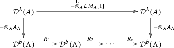
  commute up to a natural isomorphism of functors.

The vertical arrows of (1.4) induce an isomorphism $K_0({{\mathrm{per}}}\Lambda ) \rightarrow K_0(A)$ sending projectives to projectives. Thus, by considering the diagram (1.4) at the level of the Grothendieck groups, we get the following commutative diagram

(where $I_n$ is the $n \times n$ identity matrix), which explains why the theorem can be seen as a categorical interpretation of (1.1) for $B = C_{\Lambda }$, see Corollary 2.17.

To complement this result, we note that any integral square matrix B with non-negative entries and positive entries on its main diagonal can be realized as a Cartan matrix of a suitable algebra $\Lambda$ as in the theorem. More precisely, there exist a finite dimensional triangular algebra A and a triangular bimodule M over A with $B_+ = C_A$ and $B_- = C_M$, see Sect. 2.7 for the details.

1.3 Application to Serre functors

A triangular finite dimensional algebra A is of finite global dimension, hence its bounded derived category ${\mathcal {D}}^b(A)$ admits a Serre functor $\nu _A$ in the sense of Bondal and Kapranov [4]. By a result of Happel [12, I.4.6], it is given by the left derived functor of the Nakayama functor, $\nu _A = - \mathop {\otimes }\limits ^{\mathbf {L}}_A DA$. Thus, by taking in Theorem 1.2 the bimodule M to be A, we deduce the following result on the Serre functor on ${\mathcal {D}}^b(A)$.

Corollary 1.3

Let A be a finite dimensional triangular algebra over a field and let $T(A) = A \ltimes DA$ be its trivial extension algebra. Then there exist, for $1 \le i \le n={{\mathrm{rank}}}K_0(A)$, triangulated autoequivalences $R_i$ on ${\mathcal {D}}^b(T(A))$ which restrict to autoequivalences on ${{\mathrm{per}}}T(A)$, such that:

• (a) Each autoequivalence $R_i$ induces a linear map on $K_0({{\mathrm{per}}}T(A))$ whose matrix with respect to the basis of indecomposable projective T(A)-modules is given by the reflection $r_{n+1-i}^B$, where B is the symmetrization of the Cartan matrix of A;

• (b) The diagrams of triangulated functors

  

  (1.5)

  and

  

  commute up to a natural isomorphism of functors.

Thus, one can lift (a shift of) the Serre functor on ${\mathcal {D}}^b(A)$ to a product of the “reflections” $R_i$ in ${{\mathrm{per}}}T(A)$. As before, the diagram (1.5) can be regarded as a categorical interpretation of Eq. (1.3) for $C=C_A$, the Cartan matrix of A. This can be done for any upper triangular integral matrix C with non-negative entries and ones on its main diagonal, see Sect. 2.7.

1.4 On the proof

Section 2 is devoted to the proof of the theorem and its corollaries. A key ingredient in the proof is the proper definition and analysis of the functors $R_i$. They are defined, for each $1 \le i \le n$, as the left derived functors of tensoring with a two-term complex of bimodules,

$$\begin{aligned} R_i^{\Lambda } = - \mathop {\otimes }\limits ^{\mathbf {L}}_{\Lambda } \left( \Lambda e_i \otimes _k e_i \Lambda \xrightarrow {m} \Lambda \right) \end{aligned}$$

where m denotes the multiplication map and $e_1,\ldots ,e_n$ form a complete set of primitive orthogonal idempotents of $\Lambda$.

The functors $R_i^{\Lambda }$ have already been considered by Rouquier and Zimmermann [21, §4] in their construction of braid group actions on derived categories of Brauer tree algebras without exceptional vertex. In their case the algebra $\Lambda$ is a Brauer tree algebra whose tree is a Dynkin diagram of type A. Essentially the same braid group action is given by Khovanov and Seidel [16, §2.2] (see also [22, §4.3]), this time on the derived categories of certain graded algebras, denoted in their paper by $A_m$, which are closely related to the Brauer tree algebras mentioned above. The categories of modules over the algebras $A_m$ are highest weight categories and the equivalences afforded by the functors $R_i^{A_m}$ are analogs of the equivalences constructed by Rickard [20] using translation functors in the setting of representations of reductive groups in prime characteristic.

The functors $R_i^{\Lambda }$ have also been considered by Hoshino and Kato [13] in relation with constructions of two-sided tilting complexes for self-injective algebras. Moreover, when the algebra $\Lambda$ is symmetric and $\dim e_i \Lambda e_i = 2$, the functor $R_i^{\Lambda }$ can be viewed as a twist functor in the sense of Seidel and Thomas [22, §2] with respect to the 0-spherical object $e_i \Lambda$. Our result shows the importance of the functors $R_i^{\Lambda }$ for a wider class of algebras $\Lambda$, which are not necessarily restricted to be self-injective or symmetric.

In the course of the proof we first establish a special case of Theorem 1.2 where the bimodule M is zero, namely that for any finite dimensional triangular algebra A, the composition $R_n^A \cdot \ldots \cdot R_2^A \cdot R_1^A$ is isomorphic to zero on ${\mathcal {D}}^b(A)$, see Proposition 2.7. Plugging in that statement the definition of $R_i^A$, we obtain a (finite) projective resolution of the triangular algebra A as a bimodule over itself. A similar construction, with relation to Hochschild cohomology computations, was presented by Cibils in [7].

1.5 Previous work

Another categorical interpretation of (1.3), in the realm of representation theory of quivers, is given by a result of Gabriel [10], correcting previous paper by Brenner and Butler [6], relating, for a quiver without oriented cycles, the Auslander–Reiten translation on the bounded derived category of its path algebra with the composition of the reflection functors of Bernstein, Gelfand and Ponomarev [3] taken in an admissible ordering of the vertices. In Sect. 3 we provide more details and outline the differences between Gabriel’s result and our approach.

Another approach to the factorization of Serre functors for certain finite dimensional algebras, including ones arising from category ${\mathcal {O}}$ associated to semi-simple complex Lie algebras, is presented by Mazorchuk and Stroppel in [19].

2 Proof of the theorem

2.1 The building blocks: the functors $R_i^{\Lambda }$

Let $\Lambda$ be a basic finite dimensional algebra over a field k and let $P_1, \ldots , P_n$ be a complete collection of the non-isomorphic indecomposable projectives in ${{\mathrm{mod}}}\Lambda$, the category of finite dimensional right $\Lambda$-modules. Let $e_1, \ldots , e_n$ be primitive orthogonal idempotents in $\Lambda$ such that $P_i = e_i \Lambda$ for $1 \le i \le n$.

Fix $1 \le i \le n$ and consider the following complex of $\Lambda$-$\Lambda$-bimodules

$$\begin{aligned} C_i = \Lambda e_i \otimes _k e_i \Lambda \xrightarrow {m} \Lambda , \end{aligned}$$

where $\Lambda$ is in degree 0 and m is the multiplication map. Taking the tensor product $- \otimes _{\Lambda } C_i$ yields an endofunctor on the category ${\mathcal {C}}^b(\Lambda )$ of bounded complexes of finite dimensional right $\Lambda$-modules, which induces an endofunctor on its homotopy category ${\mathcal {K}}^b(\Lambda )$.

Since its terms are projective as left $\Lambda$-modules, the complex $C_i$ defines a triangulated functor

$$\begin{aligned} - \mathop {\otimes }\limits ^{\mathbf {L}}_{\Lambda } C_i = - \otimes _{\Lambda } C_i : {\mathcal {D}}^b(\Lambda )\rightarrow {\mathcal {D}}^b(\Lambda ). \end{aligned}$$

on the derived category ${\mathcal {D}}^b(\Lambda )$ of ${{\mathrm{mod}}}\Lambda$. Moreover, as the terms are also projective as right $\Lambda$-modules, this functor restricts to a functor

$$\begin{aligned} - \mathop {\otimes }\limits ^{\mathbf {L}}_{\Lambda } C_i = - \otimes _{\Lambda } C_i : {{\mathrm{per}}}\Lambda \rightarrow {{\mathrm{per}}}\Lambda \end{aligned}$$

on the triangulated subcategory ${{\mathrm{per}}}\Lambda$ of complexes quasi-isomorphic to perfect ones (that is, bounded complexes of finitely generated projectives). In the sequel, when no confusion arises, we shall denote both functors by $R^{\Lambda }_i$.

Lemma 2.1

Let $X \in {{\mathrm{mod}}}\Lambda$. Then

$$\begin{aligned} R_i^{\Lambda }(X) = {{\mathrm{Hom}}}_{\Lambda }(P_i, X) \otimes _k P_i \xrightarrow {ev} X \end{aligned}$$

where ev is the evaluation map $ev : \alpha \otimes y \mapsto \alpha (y)$.

Proof

Clearly, $X \otimes _{\Lambda } \Lambda e_i \simeq X e_i \simeq {{\mathrm{Hom}}}_{\Lambda }(e_i \Lambda , X)$. $\square$

The Grothendieck group $K_0({{\mathrm{per}}}\Lambda )$ is a free abelian group on the generators $[P_1],\ldots ,[P_n]$ equipped with a bilinear form induced by the Euler form

$$\begin{aligned} \left\langle {X}, {Y} \right\rangle _{\Lambda } = \sum _{r \in {\mathbb {Z}}} (-1)^r \dim _k {{\mathrm{Hom}}}_{{\mathcal {D}}^b(\Lambda )}(X, Y[r]) \qquad X, Y \in {{\mathrm{per}}}\Lambda . \end{aligned}$$

Corollary 2.2

Let $X \in {{\mathrm{per}}}\Lambda$. Then in $K_0({{\mathrm{per}}}\Lambda )$ we have

$$\begin{aligned} {[}R_i^{\Lambda }(X)] = [X] - \langle P_i, X \rangle _{\Lambda } [P_i] . \end{aligned}$$

Proof

Since $R_i^{\Lambda }$ is triangulated, it is enough to verify this equality on the basis elements $[P_j]$. This follows directly from Lemma 2.1. $\square$

The next lemma provides an explicit description of compositions of functors $R^{\Lambda }_i$, which will be useful in the sequel. We start by defining certain complexes of bimodules. Here and throughout the paper, when writing $\otimes$ without a subscript, we mean the tensor product over the ground field k.

Definition 2.3

Let $s \ge 1$ and let $\varphi : \{1, \ldots , s\} \rightarrow \{1, \ldots , n\}$ be any function. Define a complex $T^{\Lambda }_{\varphi }$ of $\Lambda$-$\Lambda$-bimodules by

$$\begin{aligned} T^{\Lambda }_{\varphi } = \cdots \rightarrow 0 \rightarrow T^{\Lambda ,s}_{\varphi } \xrightarrow {d^s_\varphi } \cdots \rightarrow T^{\Lambda ,r}_{\varphi } \xrightarrow {d^r_\varphi } T^{\Lambda ,r-1}_{\varphi } \rightarrow \cdots \xrightarrow {d^1_\varphi } T^{\Lambda , 0}_{\varphi } \rightarrow 0 \rightarrow \cdots \end{aligned}$$

where, for each $0 \le r \le s$, the term $T^{\Lambda ,r}_{\varphi }$ lies in degree $-r$ and

$$\begin{aligned} T^{\Lambda ,0}_\varphi = \Lambda&,&T^{\Lambda ,r}_{\varphi } = \bigoplus _{1 \le i_1< \ldots < i_r \le s} \Lambda e_{\varphi (i_1)} \otimes e_{\varphi (i_1)} \Lambda e_{\varphi (i_2)} \otimes \ldots \otimes e_{\varphi (i_r)} \Lambda \end{aligned}$$

(2.1)

with the differentials $d^r_{\varphi }$ defined on each summand by

$$\begin{aligned} d^r_{\varphi }(\lambda _0 \otimes \lambda _1 \otimes \ldots \otimes \lambda _r) = \sum _{j=0}^{r-1} (-1)^j \lambda _0 \otimes \ldots \otimes \lambda _j \lambda _{j+1} \otimes \ldots \otimes \lambda _r \end{aligned}$$

(2.2)

for $\lambda _0 \in \Lambda e_{\varphi (i_1)}$, $\lambda _r \in e_{\varphi (i_r)} \Lambda$ and $\lambda _j \in e_{\varphi (i_j)} \Lambda e_{\varphi (i_{j+1})}$ for $0< j < r$.

Lemma 2.4

In the notations of Definition 2.3, one has

$$\begin{aligned} R^{\Lambda }_{\varphi (s)} \cdot \ldots \cdot R^{\Lambda }_{\varphi (1)} = - \mathop {\otimes }\limits ^{\mathbf {L}}_{\Lambda } T^{\Lambda }_{\varphi } . \end{aligned}$$

Proof

By definition,

$$\begin{aligned} R^{\Lambda }_{\varphi (s)} \cdot \ldots \cdot R^{\Lambda }_{\varphi (2)} \cdot R^{\Lambda }_{\varphi (1)}&= \Bigl ( \ldots \Bigl ( \Bigl ( - \mathop {\otimes }\limits ^{\mathbf {L}}_{\Lambda } C_{\varphi (1)} \Bigr ) \mathop {\otimes }\limits ^{\mathbf {L}}_{\Lambda } C_{\varphi (2)} \Bigr ) \ldots \mathop {\otimes }\limits ^{\mathbf {L}}_{\Lambda } C_{\varphi (s)} \Bigr ) \\&= - \mathop {\otimes }\limits ^{\mathbf {L}}_{\Lambda } \Bigl ( C_{\varphi (1)} \otimes _{\Lambda } C_{\varphi (2)} \otimes _{\Lambda } \ldots \otimes _{\Lambda } C_{\varphi (s)} \Bigr ) \end{aligned}$$

(where we replaced $\mathop {\otimes }\limits ^{\mathbf {L}}_\Lambda$ by $\otimes _\Lambda$ since the terms of $C_i$ are projective as left (as well as right) modules), so it is enough to show that

$$\begin{aligned} T^{\Lambda }_{\varphi } = \Bigl ( \ldots \Bigl (C_{\varphi (1)} \otimes _{\Lambda } C_{\varphi (2)} \Bigr ) \otimes _{\Lambda } \ldots \otimes _{\Lambda } C_{\varphi (s)} \Bigr ) \end{aligned}$$

where the right hand side is an iterated tensor product of complexes.

We prove this by induction on s, the case $s=1$ being merely the definition of $R^{\Lambda }_{\varphi (1)}$. Now assume the claim for s, consider a function $\varphi : \{1, \ldots , s+1 \} \rightarrow \{1, \ldots , n\}$ and denote by $\varphi '$ its restriction to $\{1, \ldots , s\}$. By the induction hypothesis, we need to show that $T^{\Lambda }_{\varphi } = T^{\Lambda }_{\varphi '} \otimes _{\Lambda } C_{\varphi (s+1)}$.

Recall that the tensor product of two complexes $X_{\Lambda }$ and $_{\Lambda }Y$ is defined by

$$\begin{aligned} (X \otimes _{\Lambda } Y)^m = \bigoplus _{p+q=m} X^p \otimes _{\Lambda } Y^q \end{aligned}$$

with the differentials $d(x \otimes y) = d(x) \otimes y + (-1)^p x \otimes d(y)$ for $x \in X^p$, $y \in Y^q$. It follows that for any $0 \le r \le s+1$, the term at degree $-r$ of $T^{\Lambda }_{\varphi '} \otimes _{\Lambda } C_{\varphi (s+1)}$ equals

$$\begin{aligned} T^{\Lambda ,r}_{\varphi '} \oplus \left( T^{\Lambda ,r-1}_{\varphi '} \otimes _{\Lambda } \left( \Lambda e_{\varphi (s+1)} \otimes e_{\varphi (s+1)} \Lambda \right) \right) \end{aligned}$$

where the left summand vanishes for $r=s+1$ and the right one vanishes for $r=0$. Expanding these summands according to (2.1), we get a sum over all the r-tuples $1 \le i_1< \cdots < i_r \le s+1$, where the left summand corresponds to the tuples with $i_r \le s$ while the right one corresponds to the tuples with $i_r = s+1$. Hence the term equals $T^{\Lambda ,r}_{\varphi }$.

Concerning the differentials, we have the following picture

which shows that they coincide with the differentials $d^r_{\varphi }$ defined in (2.2). $\square$

As a side application, we show the following commutativity result which is analogous to the fact that in a Weyl group corresponding to a generalized Cartan matrix B, the two simple reflections $r^B_i$ and $r^B_j$ commute when $B_{ij} = 0 = B_{ji}$, compare with Proposition 2.12 of [22].

Lemma 2.5

If $\langle {P_i}, {P_j} \rangle _{\Lambda } = 0 = \langle {P_j}, {P_i} \rangle _{\Lambda }$ then $R^{\Lambda }_i R^{\Lambda }_j \simeq R^{\Lambda }_j R^{\Lambda }_i$.

Proof

Indeed, $R^{\Lambda }_i R^{\Lambda }_j$ and $R^{\Lambda }_j R^{\Lambda }_i$ are given by the complexes

$$\begin{aligned}&\Lambda e_j \otimes e_j \Lambda e_i \otimes e_i \Lambda \rightarrow \left( \Lambda e_j \otimes e_j \Lambda \right) \oplus \left( \Lambda e_i \otimes e_i \Lambda \right) \rightarrow \Lambda ,\\&\Lambda e_i \otimes e_i \Lambda e_j \otimes e_j \Lambda \rightarrow \left( \Lambda e_i \otimes e_i \Lambda \right) \oplus \left( \Lambda e_j \otimes e_j \Lambda \right) \rightarrow \Lambda \end{aligned}$$

which are isomorphic since $e_j \Lambda e_i = 0 = e_i \Lambda e_j$. $\square$

A special role is played by the composition $R_n^{\Lambda } \cdot \ldots \cdot R_2^{\Lambda } \cdot R_1^{\Lambda }$ corresponding to the identity function on $\{1,\ldots ,n\}$. We thus denote by $T^{\Lambda } = T^{\Lambda }_{id}$ the corresponding complex of bimodules of Definition 2.3, so that by Lemma 2.4,

$$\begin{aligned} R_n^{\Lambda } \cdot \ldots \cdot R_2^{\Lambda } \cdot R_1^{\Lambda } = - \mathop {\otimes }\limits ^{\mathbf {L}}_{\Lambda } T^{\Lambda } . \end{aligned}$$

(2.3)

2.2 Triangular algebras

In this section we study the complexes $T^A$ for triangular algebras A. Recall that a finite dimensional algebra A over a field k, with a complete set of primitive orthogonal idempotents $e_1, \ldots , e_n$, is called triangular if $e_i A e_j = 0$ for all $j < i$ and $e_i A e_i \simeq k$ for all $1 \le i \le n$ (in the literature on quasi-hereditary algebras, triangular algebras are sometimes called directed). Triangular algebras have finite global dimension, hence the categories ${{\mathrm{per}}}A$ and ${\mathcal {D}}^b(A)$ coincide.

Lemma 2.6

Let A be triangular and let $1 \le i \le j \le n$. Then

$$\begin{aligned} R_i^A(P_j) \simeq {\left\{ \begin{array}{ll} 0 &{} \text { if } j=i, \\ P_j &{} \text { if } j > i, \end{array}\right. } \end{aligned}$$

in the homotopy category ${\mathcal {K}}^b(A)$.

Proof

If $i < j$, then ${{\mathrm{Hom}}}_A(P_i, P_j) \simeq e_j A e_i = 0$, hence by Lemma 2.1, $R_i^A(P_j) = P_j$ (even in ${\mathcal {C}}^b(A)$).

Similarly, ${{\mathrm{Hom}}}_A(P_i, P_i) \simeq k$, hence $R_i^A(P_i)$ equals the null-homotopic complex $P_i \rightarrow P_i$, so it vanishes in ${\mathcal {K}}^b(A)$. $\square$

Proposition 2.7

Let A be triangular. Then:

• (a) The functor $R_n^A \cdot \ldots \cdot R_2^A \cdot R_1^A$ on ${\mathcal {D}}^b(A)$ is isomorphic to the zero functor.

• (b) $T^A \simeq 0$ in ${\mathcal {D}}^b(A^{op} \otimes A)$.

• (c) $T^A$ is contractible as a complex of right A-modules as well as a complex of left A-modules.

Proof

A repeated application of Lemma 2.6 shows that for $1 \le j, s \le n$,

$$\begin{aligned} (R^A_s \cdot \ldots \cdot R^A_1) (P_j) \simeq {\left\{ \begin{array}{ll} 0 &{} \text { if } j \le s, \\ P_j &{} \text { if } j > s, \end{array}\right. } \end{aligned}$$

in ${\mathcal {K}}^b(A)$, hence the complex $(R^A_n \cdot \ldots \cdot R^A_1)(A)$ is homotopic to zero. Since A generates ${\mathcal {D}}^b(A)$, the first assertion follows. Now the second assertion follows from (2.3). For the third, observe that all the terms of $T^A$ are projective both as right and as left A-modules (in fact, the above argument shows directly the contractibility of $T^A$ as a complex of right A-modules). $\square$

Remark 2.8

Since all its terms at negative degrees are also projective as A-A-bimodules, the complex $T^A$ yields a projective resolution of A as an A-A-bimodule, which can be useful when computing Hochschild cohomology. Indeed, a similar resolution is given by Cibils [7], where an explicit contraction (of k-modules) is also given.

Remark 2.9

Since $T^A$ is contractible as a complex of left A-modules, the tensor product $X \otimes _A T^A$ yields a projective resolution of a right module $X_A$. Similarly, $T^A \otimes _A Y$ gives a projective resolution of a left module $_AY$.

The statement of Proposition 2.7 is no longer true when the assumption that A is triangular is removed, even under the condition that A has finite global dimension. This is demonstrated by the following example.

Example 2.10

Let $\Lambda$ be the path algebra of the quiver

modulo the ideal generated by the path $\beta \alpha$. The algebra $\Lambda$ is 5-dimensional, its primitive orthogonal idempotents $e_1, e_2$ correspond to the vertices of the quiver and its global dimension is 2. However, $\Lambda$ is not triangular as its Cartan matrix equals

$$\begin{aligned} \begin{pmatrix} 2 &{}\quad 1 \\ 1 &{}\quad 1 \end{pmatrix} . \end{aligned}$$

Moreover, the complex

$$\begin{aligned} T^{\Lambda } = \Bigl ( \Lambda e_1 \otimes e_1 \Lambda e_2 \otimes e_2 \Lambda \rightarrow \left( \Lambda e_1 \otimes e_1 \Lambda \right) \oplus \left( \Lambda e_2 \otimes e_2 \Lambda \right) \rightarrow \Lambda \Bigr ) \end{aligned}$$

is not acyclic since its Euler characteristic as a complex of vector spaces (that is, the alternating sum of dimensions) is $3 \cdot 1 \cdot 2 - (3 \cdot 3 + 2 \cdot 2) + 5 \ne 0$.

Note that when $k={\mathbb {C}}$, the category ${{\mathrm{mod}}}\Lambda$ is equivalent to the principal block of category ${\mathcal {O}}$ of the complex Lie algebra $\mathfrak {sl}_2$, see [23, §5.1.1].

For a triangular algebra A, the compositions of $R^A_i$ in the reverse order have a very simple form. This is recorded in the next proposition, which will not be used in the sequel.

Proposition 2.11

Let A be triangular. Let $I \subseteq \{1,\ldots ,n\}$ and enumerate its elements in decreasing order $I = \{i_1> i_2> \cdots > i_s\}$. Then

$$\begin{aligned} R^A_{i_s} \cdot \ldots \cdot R^A_{i_1} = - \mathop {\otimes }\limits ^{\mathbf {L}}_A \Bigl ( \bigoplus _{i \in I} A e_i \otimes e_i A \xrightarrow {m} A \Bigr ) \end{aligned}$$

Proof

Apply Lemma 2.4 for the function $\varphi$ defined by $\varphi (t) = i_t$ for $1 \le t \le s$ and observe that all the terms $T^{A,r}_{\varphi }$ vanish when $r > 1$ as $e_{i_t} A e_{i_{t+1}} = 0$ for all $1 \le t < s$. $\square$

2.3 Triangular bimodules and their trivial extensions

Let A be a basic finite dimensional algebra with a complete set $e_1, \ldots , e_n$ of primitive orthogonal idempotents.

Let M be an A-A-bimodule and let $DM = {{\mathrm{Hom}}}_k(M,k)$ be its dual. Consider the trivial extension $\Lambda = A \ltimes DM$, that is, the k-algebra which has $A \oplus DM$ as an underlying vector space, with the multiplication defined by $(a,\mu ) (a',\mu ') = (aa', a \mu ' + \mu a')$.

The ring homomorphisms $A \xrightarrow {\iota } \Lambda \xrightarrow {\pi } A$ given by

$$\begin{aligned} \iota (a) = (a,0) \qquad \qquad \pi (a,\mu ) = a \end{aligned}$$

give rise to the bimodules $_A{\Lambda }_A$ and $_{\Lambda }A_{\Lambda }$ (where $a \in A$ acts via multiplication by $\iota (a)$ and $\lambda \in \Lambda$ acts via multiplication by $\pi (\lambda )$). In particular we have the exact functors

$$\begin{aligned} \iota ^{*}&= - \otimes _\Lambda \Lambda _A = {{\mathrm{Hom}}}_{\Lambda }({_A{\Lambda }_{\Lambda }}, -) : {{\mathrm{mod}}}\Lambda \rightarrow {{\mathrm{mod}}}A \\ \pi ^{*}&= - \otimes _A A_{\Lambda } = {{\mathrm{Hom}}}_A ({_{\Lambda }A_A}, -) : {{\mathrm{mod}}}A \rightarrow {{\mathrm{mod}}}\Lambda \end{aligned}$$

which induce functors

$$\begin{aligned} {\mathcal {D}}^b(\Lambda )\xrightarrow {- \otimes _{\Lambda } \Lambda _A} {\mathcal {D}}^b(A), \quad {\mathcal {D}}^b(A)\xrightarrow {- \otimes _A A_{\Lambda }} {\mathcal {D}}^b(\Lambda ). \end{aligned}$$

The left derived functors of their adjoints

$$\begin{aligned} - \otimes _A \Lambda _{\Lambda } : {{\mathrm{mod}}}A \rightarrow {{\mathrm{mod}}}\Lambda , \quad - \otimes _{\Lambda } A_A : {{\mathrm{mod}}}\Lambda \rightarrow {{\mathrm{mod}}}A . \end{aligned}$$

give rise to

$$\begin{aligned} {\mathcal {D}}^b(A)= {{\mathrm{per}}}A \xrightarrow {- \mathop {\otimes }\limits ^{\mathbf {L}}_A \Lambda _{\Lambda }} {{\mathrm{per}}}\Lambda , \quad {{\mathrm{per}}}\Lambda \xrightarrow {- \mathop {\otimes }\limits ^{\mathbf {L}}_{\Lambda } A_A} {{\mathrm{per}}}A = {\mathcal {D}}^b(A). \end{aligned}$$

The elements $\iota (e_1),\ldots ,\iota (e_n)$ form a complete set of primitive orthogonal idempotents of $\Lambda$. We shall denote them by $e_1,\ldots ,e_n$ when there is no risk of confusion.

We say that the bimodule M is triangular if $e_i M e_j = 0$ for all $j < i$.

Proposition 2.12

Let A be a finite dimensional basic algebra, let M be a triangular bimodule and let $\Lambda = A \ltimes DM$. Then there exist short exact sequences of complexes of bimodules

$$\begin{aligned} {\begin{matrix} 0 \rightarrow {_{\Lambda }DM_A} \rightarrow \Lambda \otimes _A T^A \rightarrow T^{\Lambda } \otimes _{\Lambda } A \rightarrow 0 \\ 0 \rightarrow {_ADM_{\Lambda }} \rightarrow T^A \otimes _A \Lambda \rightarrow A \otimes _{\Lambda } T^{\Lambda } \rightarrow 0 \end{matrix}} \end{aligned}$$

(2.4)

Proof

We prove only the exactness of the first sequence, as the proof for the other is similar.

Let $1 \le r \le n$ and consider the terms in degree $-r$ of $\Lambda \otimes _A T^A$ and $T^{\Lambda } \otimes _{\Lambda } A$ as direct sums

$$\begin{aligned} \bigl ( \Lambda \otimes _A T^A \bigr )^{-r}&= \bigoplus \Lambda e_{i_1} \otimes e_{i_1} A e_{i_2} \otimes \ldots \otimes e_{i_{r-1}} A e_{i_r} \otimes e_{i_r} A \\ \bigl ( T^{\Lambda } \otimes _{\Lambda } A \bigr )^{-r}&= \bigoplus \Lambda e_{i_1} \otimes e_{i_1} \Lambda e_{i_2} \otimes \ldots \otimes e_{i_{r-1}} \Lambda e_{i_r} \otimes e_{i_r} A \end{aligned}$$

running over the tuples $1 \le i_1< \cdots < i_r \le n$.

By our hypothesis that M is a triangular bimodule, $e_j M e_i = 0$ hence $e_i DM e_j = 0$ for all $i < j$. Therefore we can identify $e_i A e_j$ with $e_i \Lambda e_j$ (via either $\iota$ or $\pi$) so that the terms $(\Lambda \otimes _A T^A)^{-r}$ and $(T^{\Lambda } \otimes _{\Lambda } A)^{-r}$ are isomorphic via the map

$$\begin{aligned} \lambda _0 \otimes a_1 \otimes \cdots \otimes a_{r-1} \otimes a_r \mapsto \lambda _0 \otimes \iota (a_1) \otimes \cdots \otimes \iota (a_{r-1}) \otimes a_r . \end{aligned}$$

Moreover, by considering the explicit forms of the right A-action on $\Lambda$ and the left $\Lambda$-action on A,

$$\begin{aligned} \lambda _0 \cdot a_1 = \lambda _0 \iota (a_1)&,&a_{r-1}a_r = \iota (a_{r-1}) \cdot a_r&,&\iota (a_j a_{j+1}) = \iota (a_j) \iota (a_{j+1}) \end{aligned}$$

for $1 \le j < r-1$, we see that these isomorphisms commute with the differentials as long as $r > 1$.

Finally, note that $(\Lambda \otimes _A T^A)^0 = \Lambda$, $(T^{\Lambda } \otimes _{\Lambda } A)^0 = A$ and there is a commutative diagram

with the top and bottom differentials given by

$$\begin{aligned} d^{A,1} : \lambda _i \otimes a_i \mapsto \lambda _i \iota (a_i) \in \Lambda ,\qquad d^{\Lambda ,1} : \lambda _i \otimes a_i \mapsto \pi (\lambda _i) a_i \in A \end{aligned}$$

respectively.

Summarizing, we get the following commutative diagram of complexes of A-$\Lambda$-bimodules which shows the desired exact sequence.

$\square$

2.4 Proof of Theorem 1.2

Let A be a triangular algebra with a complete set $e_1, \ldots , e_n$ of primitive orthogonal idempotents and let M be a triangular A-A-bimodule (with respect to this ordering of the idempotents). By combining Propositions 2.7 and 2.12 we deduce the next result.

Corollary 2.13

Let $\Lambda = A \ltimes DM$. We have

$$\begin{aligned} T^{\Lambda } \otimes _{\Lambda } A \xrightarrow {\sim } DM[1] \quad and \quad A \otimes _{\Lambda } T^{\Lambda } \xrightarrow {\sim } DM[1] \end{aligned}$$

in ${\mathcal {D}}^b(\Lambda ^{op} \otimes A)$ and ${\mathcal {D}}^b(A^{op} \otimes \Lambda )$, respectively.

Proof

Since $T^A$ is contractible as a complex of left A-modules, the complex $\Lambda \otimes _A T^A$ is contractible as a complex of left $\Lambda$-modules, hence it is isomorphic to zero in ${\mathcal {D}}^b(\Lambda ^{op} \otimes A)$. Now the assertion follows from the first short exact sequence in (2.4). The proof of the second assertion is similar. $\square$

Part (b) of Theorem 1.2 now follows from Corollary 2.13 by setting $R_i = R^{\Lambda }_i$ for $1 \le i \le n$ and using (2.3).

Remark 2.14

When M is zero, $\Lambda = A$ and we recover Proposition 2.7.

2.5 K-theoretic interpretation

We now prove part (a) of Theorem 1.2 and explain how that theorem can be regarded as a categorification of Eq. (1.1). In fact, we will recover this equation through a process known as decategorification, by looking at the effect of the functors appearing in the theorem on the corresponding Grothendieck groups.

Indeed, as the functors $R_i^{\Lambda }$, $- \mathop {\otimes }\limits ^{\mathbf {L}}_A DM_A[1]$ and $- \mathop {\otimes }\limits ^{\mathbf {L}}_{\Lambda } A$ are triangulated, they induce linear maps on the corresponding Grothendieck groups, which we describe explicitly in terms of the Cartan matrices of A and $\Lambda$.

For an arbitrary (basic) finite dimensional algebra $\Lambda$ with indecomposable projectives $P_1, \ldots , P_n$, it will be convenient to reorder them in reverse order and to consider the basis

$$\begin{aligned} \varepsilon _1 = [P_n], \varepsilon _2 = [P_{n-1}], \ldots , \varepsilon _n = [P_1] \end{aligned}$$

of the Grothendieck group $K_0({{\mathrm{per}}}\Lambda )$. We denote by $C_{\Lambda }$ the matrix of the Euler form $\left\langle {\cdot }, {\cdot } \right\rangle _{\Lambda }$ with respect to that basis, known as the Cartan matrix of $\Lambda$. In explicit terms,

$$\begin{aligned} (C_{\Lambda })_{ij}&= \left\langle {P_{n+1-i}}, {P_{n+1-j}} \right\rangle _{\Lambda } = \dim _k {{\mathrm{Hom}}}_{\Lambda }(P_{n+1-i}, P_{n+1-j}) \\&= \dim _k e_{n+1-j} \Lambda e_{n+1-i} . \end{aligned}$$

Lemma 2.15

Let $1 \le i \le n$. Then the matrix of the linear map on $K_0({{\mathrm{per}}}\Lambda )$ induced by $R_i^{\Lambda }$ is given by $r^{C_{\Lambda }}_{n+1-i}$.

Proof

The j-th column of that matrix is equal to the class of $R^{\Lambda }_i(P_{n+1-j})$ in $K_0({{\mathrm{per}}}\Lambda )$ which, according to Corollary 2.2, equals

$$\begin{aligned}{}[R^{\Lambda }_i(P_{n+1-j})] = [P_{n+1-j}] - \left\langle {P_i}, {P_{n+1-j}} \right\rangle _{\Lambda }[P_i] = \varepsilon _j - (C_{\Lambda })_{n+1-i,j} \varepsilon _{n+1-i} . \end{aligned}$$

$\square$

For an algebra A with a complete set $e_1, \ldots , e_n$ of primitive orthogonal idempotents, the condition that A is triangular implies that the matrix $C_A$ is upper triangular with ones on its main diagonal. Similarly to the definition of $C_A$, one can define for any A-A-bimodule X, a Cartan matrix $C_X$ by

$$\begin{aligned} (C_X)_{ij} = \dim _k e_{n+1-j} X e_{n+1-i} , \end{aligned}$$

so that X is triangular if and only if $C_X$ is upper triangular.

Lemma 2.16

Let A be a triangular algebra and X an A-A-bimodule. Then the matrix of the linear map on $K_0({{\mathrm{per}}}A)$ induced by the functor $- \mathop {\otimes }\limits ^{\mathbf {L}}_A X$ is given by $C_A^{-1} C_X$.

Proof

Denote that matrix (with respect to the basis $\varepsilon _1,\ldots ,\varepsilon _n$) by x. Since the functor $- \mathop {\otimes }\limits ^{\mathbf {L}}_A X$ sends each $P_j$ to $P_j \otimes _A X \simeq e_j X$, we have

$$\begin{aligned}{}[e_{n+1-j} X] = \sum _{i=1}^n x_{ij} [P_{n+1-i}] \end{aligned}$$

for all $1 \le j \le n$. Now, for any $1 \le l \le n$,

$$\begin{aligned} (C_X)_{lj}&= \dim _k e_{n+1-j} X e_{n+1-l} = \left\langle {P_{n+1-l}}, {e_{n+1-j}X} \right\rangle _A \\&= \sum _{i=1}^n x_{ij} \left\langle {P_{n+1-l}}, {P_{n+1-i}} \right\rangle _A = \sum _{i=1}^n (C_A)_{li} x_{ij} , \end{aligned}$$

hence $C_X = C_A x$. $\square$

When A is triangular and M is a triangular bimodule, the Cartan matrix of the trivial extension $\Lambda = A \ltimes DM$ equals $C_{\Lambda } = C_A + C_{DM} = C_A + C_M^T$. Hence $(C_{\Lambda })_{+} = C_A$ is the upper triangular part of $C_{\Lambda }$ and $(C_{\Lambda })_{-} = C_M$ is its lower triangular part, as defined in Proposition 1.1.

Combining everything together, observing that the functor $- \mathop {\otimes }\limits ^{\mathbf {L}}_{\Lambda } A$ sends the projective $\iota (e_i) \Lambda$ to $e_i A$ and thus induces the identity matrix between the isomorphic groups $K_0({{\mathrm{per}}}\Lambda )$ and $K_0({{\mathrm{per}}}A)$, we conclude the following.

Corollary 2.17

The diagram (1.4) of Theorem 1.2 induces a commutative diagram on the Grothendieck groups

(where $I_n$ is the $n \times n$ identity matrix), thus recovering Eq. (1.1) for $B= C_{\Lambda }$.

2.6 Proof of Corollary 1.3

Let $e_1,\ldots ,e_n$ be a complete set of primitive orthogonal idempotents of A and set $R_i = R^{T(A)}_i$ for $1 \le i \le n$.

The algebra T(A) is symmetric and $\dim _k e_i T(A) e_i = 2$ for any $1 \le i \le n$. Hence by [13, Remark 4.3], the functors $R^{T(A)}_i$ are autoequivalences, see also [21, Theorem 4.1].

Since $\nu _A = - \mathop {\otimes }\limits ^{\mathbf {L}}_A DA$ and $A \ltimes DA = T(A)$, Corollary 1.3 is just a special case of Theorem 1.2, where the triangular bimodule M is taken to be A.

Remark 2.18

The Cartan matrix B of T(A) is symmetric with 2 on its main diagonal, hence the matrices $r^B_i$ are reflections. As the action of each autoequivalence $R^{T(A)}_i$ on $K_0({{\mathrm{per}}}T(A))$ is given by a reflection, one may interpret this corollary as lifting of the Serre functor (up to a shift by one) on ${\mathcal {D}}^b(A)$ to a product of “reflection” functors on ${{\mathrm{per}}}T(A)$.

2.7 Realization of matrices as Cartan matrices

We now show that Theorem 1.2 categorifies (1.1) for any integral square matrix B with non-negative entries and positive entries on its main diagonal. We start with an observation on the realization of such matrices as Cartan matrices of finite dimensional algebras.

Lemma 2.19

Let C be an integral $n \times n$ matrix with $C_{ij} \ge 0$ and $C_{ii} > 0$ for $1 \le i, j \le n$, and let k be a field. Then there exists a finite dimensional algebra A over k whose Cartan matrix equals C.

Proof

We construct A from a quiver with relations. Let Q be the quiver whose vertices are $\{1, 2, \ldots , n\}$, with the number of arrows from i to j set to

$$\begin{aligned} \left| \{\text {arrows } i \rightarrow j \}\right| = C_{n+1-j,n+1-i} - \delta _{ij} . \end{aligned}$$

Let $I \subseteq kQ$ be the ideal in the path algebra of Q generated by all the paths of length 2. Then the Cartan matrix of $A = kQ/I$ equals C, since $\dim _k {{\mathrm{Hom}}}_A(P_{n+1-i}, P_{n+1-j})$ is the number of paths in Q from $n+1-j$ to $n+1-i$ of length at most one, which equals $C_{ij}$ by construction. $\square$

Observe that the algebra A constructed in the lemma is triangular if and only if the square matrix C with non-negative integer entries is upper triangular with ones on its main diagonal. Hence Corollary 1.3 categorifies (1.3) for any such matrix C (or equivalently, for any square symmetric matrix B with non-negative integer entries and 2 on its main diagonal).

We now consider the realization of bimodules with prescribed Cartan matrix.

Lemma 2.20

Let $C'$ be an integral $n \times n$ matrix with non-negative entries and A a finite dimensional algebra as constructed in the previous lemma. Then there exists a bimodule M over A such that $C_M = C'$.

Proof

Let $A = kQ/I$ be as in the previous lemma. For each $1 \le i \le n$, let $S_i$ (respectively, $S'_i$) denote the simple right (respectively, left) A-module corresponding to the vertex i in Q. Then $S'_j \otimes _k S_i$ is a one dimensional simple A-A-bimodule for any $1 \le i,j \le n$.

Let $M = \bigoplus _{1 \le i,j \le n} (S'_j \otimes _k S_i)^{\oplus C'_{n+1-i,n+1-j}}$. Then M is a bimodule over A such that $C_M = C'$, since

$$\begin{aligned} (C_M)_{ij}&= \dim _k e_{n+1-j} M e_{n+1-i} \\&= \dim _k (S'_{n+1-j} \otimes S_{n+1-i})^{\oplus C'_{n+1-(n+1-i),n+1-(n+1-j)}} = C'_{ij} \end{aligned}$$

for any $1 \le i,j \le n$. $\square$

Combining the above two observations, we deduce the following.

Corollary 2.21

Let B be an integral $n \times n$ matrix with $B_{ij} \ge 0$ and $B_{ii} > 0$ for $1 \le i, j \le n$, and let k be a field. Then there exist a finite dimensional triangular algebra A over k and a triangular bimodule M over A such that $C_A = B_+$ and $C_M = B_-$. In particular, $B = C_{\Lambda }$ for $\Lambda = A \ltimes DM$.

Proof

Use Lemma 2.19 with $C=B_{+}$ to construct the algebra A, and then Lemma 2.20 with $C'=B_{-}$ to construct the bimodule M. $\square$

3 Discussion and comparison

In this section we recall previous work on path algebras of quivers that can also be considered as a categorical interpretation of Eq. (1.3), and compare it with our approach.

3.1 A result of Gabriel

Fix an algebraically closed field k. For a quiver Q without oriented cycles, denote by kQ its path algebra and by ${\mathcal {D}}^b(Q)$ the bounded derived category of finite dimensional right kQ-modules. Recall that a vertex $s \in Q$ is called a sink if there are no arrows in Q starting at s. The reflection of Q at s, denoted $\sigma _s Q$, is the quiver obtained from Q by inverting all the arrows ending at s while leaving all the others intact, so that s becomes a source in $\sigma _s Q$.

In [3], Bernstein, Gelfand and Ponomarev defined the reflection functor from the category of representations of Q to those of $\sigma _s Q$ (where s is a sink in Q). In the language of derived categories (see for example [11, (IV.4, Exercise 6)]), this functor induces a derived equivalence

$$\begin{aligned} R_s : {\mathcal {D}}^b(Q)\xrightarrow {\sim } {\mathcal {D}}^b(\sigma _s Q) . \end{aligned}$$

Order now the vertices of Q in an admissible ordering, that is, enumerate them in a sequence $1,2,\ldots , n$ such that there are no arrows $j \rightarrow i$ in Q for $i < j$. In this case, the vertex $1 \le i \le n$ is a sink in the quiver $\sigma _{i+1} \sigma _{i+2} \ldots \sigma _n Q$. Moreover, the quiver $\sigma _1 \ldots \sigma _n Q$ is equal to Q. Thus, the composition of the (derived) reflection functors

$$\begin{aligned} {\mathcal {D}}^b(Q)\xrightarrow {R_n} {\mathcal {D}}^b(\sigma _n Q) \xrightarrow {R_{n-1}} {\mathcal {D}}^b(\sigma _{n-1} \sigma _n Q) \xrightarrow {R_{n-2}} \cdots \xrightarrow {R_1} {\mathcal {D}}^b(\sigma _1 \ldots \sigma _n Q) \end{aligned}$$

defines an autoequivalence $R_1 \cdot R_2 \cdot \ldots \cdot R_n$ of ${\mathcal {D}}^b(Q)$, known as the Coxeter functor.

The following result of Gabriel [10] compares the Coxeter functor with another autoequivalence on ${\mathcal {D}}^b(Q)$ given by the Auslander–Reiten translation $\tau$ which can be written as $\tau = -\mathop {\otimes }\limits ^{\mathbf {L}}_{kQ} D(kQ)[-1]$ by [12, I.4.6].

Theorem 3.1

[10, §5] If the underlying graph of Q is a tree, or more generally, does not contain a cycle of odd length, then

$$\begin{aligned} \tau \simeq R_1 \cdot R_2 \cdot \ldots \cdot R_n . \end{aligned}$$

(3.1)

Similarly to Corollary 2.17, the relation with Eq. (1.3) is obtained through decategorification by considering the Grothendieck group $K_0(Q)$ of the triangulated category ${\mathcal {D}}^b(Q)$ together with its Euler form $\left\langle {\cdot }, {\cdot } \right\rangle _{kQ}$, but this time using bases of simple modules rather than the indecomposable projective ones.

Let $S_i$ be the simple module corresponding to the vertex $1 \le i \le n$. The classes $[S_1], \ldots , [S_n]$ form a basis of $K_0(Q)$, and the matrix $C_Q$ of $\left\langle {\cdot }, {\cdot } \right\rangle _{kQ}$ with respect to that basis has an explicit combinatorial description, namely

$$\begin{aligned} (C_Q)_{ij} = \delta _{ij} -\bigl | \{\text {arrows } i \rightarrow j\} \bigr | . \end{aligned}$$

When the vertices are ordered in an admissible order, the matrix $C_Q$ is upper triangular with ones on its main diagonal.

Given a sink s, the reflection functor $R_s$ induces a linear map $K_0(Q) \rightarrow K_0(\sigma _s Q)$ whose matrix with respect to the bases of simples is given by the reflection $r_s^{B_Q}$, where $B_Q = C_Q + C_Q^T$ is the symmetrization of $C_Q$, see [3]. Moreover, $B_{\sigma _s Q} = B_Q$ since

$$\begin{aligned} (B_Q)_{ij} = 2 \delta _{ij} - \bigl | \{\text {arrows } i \rightarrow j\} \bigr | - \bigl |\{\text {arrows } j \rightarrow i\} \bigr | \end{aligned}$$

is independent on the orientation of the arrows.

On the other hand, it is well known that the matrix of the linear map on $K_0(Q)$ induced by $\tau$ is given by $-C_Q^{-1} C_Q^T$. Therefore, Theorem 3.1 implies the following commutative diagram

recovering Eq. (1.3) for $C=C_Q$ as a K-theoretical consequence of the isomorphism of the functors $\tau$ and $R_1 \cdot R_2 \cdot \ldots \cdot R_n$ on ${\mathcal {D}}^b(Q)$.

3.2 Comparison

It had been claimed in [6] that (3.1) holds for any quiver without oriented cycles, however this turned out to be false, see [10, §5.4]. As Theorem 1.2 deals with arbitrary triangular algebras and in particular with all such quivers, the reader might wonder how one can generalize an incorrect statement. The answer to this puzzle is that Theorem 1.2 (and its Corollary 1.3) are not generalizations of Theorem 3.1 (i.e. the functors occurring in the statements are different), so while both results can be regarded as categorical interpretations of Eqs. (1.1) and (1.3), one notices several differences, as outlined below.

Compared with Theorem 3.1, Theorem 1.2 has broader scope in two aspects; firstly, it applies to any finite dimensional triangular algebra A, and not only to hereditary ones. Secondly, it applies to any triangular bimodule M, and not only to $M=A$, thus providing an interpretation of Eq. (1.1) rather than the more specific (1.3). This broader scope carries some price to be paid, namely that while Theorem 3.1 provides a factorization of the Auslander–Reiten translation as a composition of reflection functors, Theorem 1.2 does not factor $- \mathop {\otimes }\limits ^{\mathbf {L}}_A DM[1]$, but rather provides only a factorization of a lift to ${{\mathrm{per}}}\Lambda$ for $\Lambda = A \ltimes DM$.

In both results, the minus sign in the left hand side of (1.1) and (1.3) is interpreted as a shift applied to the functor of tensoring with a bimodule. However, in Theorem 1.2 this is a positive shift, while in Theorem 3.1 it is a negative one. Clearly, they are indistinguishable in the Grothendieck group.

Finally, both Corollary 1.3 and Theorem 3.1 categorify the same statement, namely Eq. (1.3), and in both cases the upper triangular matrix C is the matrix of the Euler form with respect to some basis. However, in Corollary 1.3 this is the basis of indecomposable projectives, while in Theorem 3.1 it is the basis of simple modules.

The use of the basis of simple modules is a rather special feature of hereditary algebras. Indeed, for a quiver Q and a sink s, one has $C_{\sigma _s Q} = r_s^T C_Q r_s$ where $r_s$ is the corresponding reflection built from the symmetrization of $C_Q$. However, as the next example illustrates, if A is a triangular algebra whose Euler form is given by an upper triangular matrix C with respect to the basis of simple modules and if s is a sink or a source in the quiver of A, then in general there may not exist an algebra whose Euler form with respect to the basis of simple modules is given by the matrix $r^T_s C r_s$, where $r_s$ is the reflection built from the symmetrization of C.

Example 3.2

Let A be the algebra given by the quiver

modulo the relation $\alpha \beta = 0$. The matrix of its Euler form with respect to the basis of simple modules $\{S_1, S_2, S_3\}$ is

$$\begin{aligned} C = \begin{pmatrix} 1 &{}\quad -1 &{}\quad 1 \\ 0 &{}\quad 1 &{}\quad -1 \\ 0 &{}\quad 0 &{}\quad 1 \end{pmatrix} , \end{aligned}$$

and the reflections built from the symmetrization $B = C + C^T$ are

$$\begin{aligned} r_1 = \begin{pmatrix} -1 &{}\quad 1 &{}\quad -1 \\ 0 &{}\quad 1 &{}\quad 0 \\ 0 &{}\quad 0 &{}\quad 1 \end{pmatrix}&,&r_2 = \begin{pmatrix} 1 &{}\quad 0 &{}\quad 0 \\ 1 &{}\quad -1 &{}\quad 1 \\ 0 &{}\quad 0 &{}\quad 1 \end{pmatrix}&,&r_3 = \begin{pmatrix} 1 &{}\quad 0 &{}\quad 0 \\ 0 &{}\quad 1 &{}\quad 0 \\ -1 &{}\quad 1 &{}\quad -1 \end{pmatrix}. \end{aligned}$$

The matrices $r_1^T C r_1$ and $r_3^T C r_3$ cannot represent Euler forms of algebras with respect to bases of simple modules. Indeed, if this were the case then their inverses would be Cartan matrices of algebras, which is impossible since

$$\begin{aligned} \left( r_1^T C r_1 \right) ^{-1} = \begin{pmatrix} 1 &{}\quad 0 &{}\quad 0 \\ 0 &{}\quad 1 &{}\quad 1 \\ -1 &{}\quad 0 &{}\quad 1 \end{pmatrix}&,&\left( r_3^T C r_3 \right) ^{-1} = \begin{pmatrix} 1 &{}\quad 1 &{}\quad 0 \\ 0 &{}\quad 1 &{}\quad 0 \\ -1 &{}\quad 0 &{}\quad 1 \end{pmatrix} \end{aligned}$$

contain negative entries.

References

A’Campo, N.: Sur les valeurs propres de la transformation de Coxeter. Invent. Math. 33(1), 61–67 (1976)
Baez, J.C., Dolan, J.: Categorification, higher category theory (Evanston, IL, 1997). Contemporary mathematics, vol. 230. American Mathematical Society, Providence, 1998, pp. 1–36
Bernstein, I.N., Gel’fand, I.M., Ponomarev, V.A.: Coxeter functors and Gabriel’s theorem. Russ. Math. Surv. 28(2), 17–32 (1973)
Bondal, A.I., Kapranov, M.M.: Representable functors, Serre functors, and reconstructions. Izv. Akad. Nauk SSSR Ser. Mat. 53(6), 1183–1205 (1989). 1337
Bourbaki, N.: Lie groups and Lie algebras. Chapters 4–6, Elements of mathematics. Springer, Berlin, 2002. Translated from the 1968 French original by Andrew Pressley
Brenner, S., Butler, M.C.R.: The equivalence of certain functors occurring in the representation theory of Artin algebras and species. J. London Math. Soc. 14(1), 183–187 (1976)
Cibils, C.: Cohomology of incidence algebras and simplicial complexes. J. Pure Appl. Algebra 56(3), 221–232 (1989)
Coleman, A.J.: Killing and the Coxeter transformation of Kac–Moody algebras. Invent. Math. 95(3), 447–477 (1989)
Coxeter, H.S.M.: The product of the generators of a finite group generated by reflections. Duke Math. J. 18, 765–782 (1951)
Gabriel, P.: Auslander–Reiten sequences and representation-finite algebras, representation theory, I. In: Proceedings on Workshop, Carleton University, Ottawa, ON, 1979. Lecture Notes in Mathematics, vol. 831, pp. 1–71. Springer, Berlin (1980)
Gelfand, S.I., Manin, Y.I.: Methods of Homological Algebra. Springer Monographs in Mathematics, Second edn. Springer, Berlin (2003)
Happel, D.: Triangulated Categories in the Representation Theory of Finite-Dimensional Algebras, London Mathematical Society Lecture Note Series, vol. 119. Cambridge University Press, Cambridge (1988)
Hoshino, M., Kato, Y.: Tilting complexes defined by idempotents. Comm. Algebra 30(1), 83–100 (2002)
Howlett, R.B.: Coxeter groups and \(M\)-matrices. Bull. London Math. Soc. 14(2), 137–141 (1982)
Khovanov, M., Mazorchuk, V., Stroppel, C.: A categorification of integral Specht modules. Proc. Am. Math. Soc. 136(4), 1163–1169 (2008)
Khovanov, M., Seidel, P.: Quivers, Floer cohomology, and braid group actions. J. Am. Math. Soc. 15(1), 203–271 (2002)
Ladkani, S.: On the periodicity of Coxeter transformations and the non-negativity of their Euler forms. Linear Algebra Appl. 428(4), 742–753 (2008)
Lenzing, H.: Coxeter transformations associated with finite-dimensional algebras. Computational methods for representations of groups and algebras (Essen, 1997), Progr. Math., vol. 173, pp. 287–308. Birkhäuser, Basel (1999)
Mazorchuk, V., Stroppel, C.: Projective-injective modules, Serre functors and symmetric algebras. J. Reine Angew. Math. 616, 131–165 (2008)
Rickard, J.: Translation functors and equivalences of derived categories for blocks of algebraic groups. Finite-dimensional algebras and related topics (Ottawa, ON, 1992), NATO Adv. Sci. Inst. Ser. C Math. Phys. Sci., vol. 424, pp. 255–264. Kluwer Acad. Publ., Dordrecht (1994)
Rouquier, R., Zimmermann, A.: Picard groups for derived module categories. Proc. London Math. Soc. 87(1), 197–225 (2003)
Seidel, P., Thomas, R.: Braid group actions on derived categories of coherent sheaves. Duke Math. J. 108(1), 37–108 (2001)
Stroppel, C.: Category \({\cal O}\): quivers and endomorphism rings of projectives. Represent. Theory 7, 322–345 (2003)
Acknowledgements
Open access funding provided by Max Planck Society. The results in this paper were first presented at the workshop on Spectral methods in representation theory of algebras and applications to the study of rings of singularities that was held at Banff in September 2008. I would like to thank J. A. de la Peña, C. Ringel and C. Stroppel for their helpful comments and suggestions. I would also like to thank the anonymous referee for the helpful comments.
Author information
Authors and Affiliations
Corresponding author
Rights and permissions
Open Access This article is distributed under the terms of the Creative Commons Attribution 4.0 International License (http://creativecommons.org/licenses/by/4.0/), which permits unrestricted use, distribution, and reproduction in any medium, provided you give appropriate credit to the original author(s) and the source, provide a link to the Creative Commons license, and indicate if changes were made.
About this article
Cite this article
Ladkani, S. Categorification of a linear algebra identity and factorization of Serre functors. Math. Z. 285, 879–896 (2017). https://doi.org/10.1007/s00209-016-1731-9
Received:
Accepted:
Published:
Issue Date:
DOI: https://doi.org/10.1007/s00209-016-1731-9