Simplified group activity selection with group size constraints

Abstract

Several real-world situations can be represented in terms of agents that have preferences over activities in which they may participate. Often, the agents can take part in at most one activity (for instance, since these take place simultaneously), and there are additional constraints on the number of agents that can participate in an activity. In such a setting, we consider the task of assigning agents to activities in a reasonable way. We introduce the simplified group activity selection problem providing a general yet simple model for a broad variety of settings, and start investigating its special case where upper and lower bounds of the groups have to be taken into account. We apply different solution concepts such as envy-freeness and core stability to our setting and provide a computational complexity study for the problem of finding such solutions.

1 Introduction

Several real-world situations can be represented in terms of agents that have preferences over activities in which they may participate, subject to some feasibility constraints on the way they are assigned to the different activities. In many scenarios, agents can take part in at most one activity (e.g., since these take place simultaneously), which is the setting considered in this work. In this respect, ‘activity’ should be taken in a wide sense; typical examples include, for instance, tasks, coalitions, or courses.

The group activity selection problem (GASP) asks how to assign agents to activities in a “good” way. In the original form introduced by Darmann et al. (2012, 2018), agents express their preferences both on the activities and on the number of participants for the latter; in general, these preferences are expressed by means of weak orders over pairs “(activity, group size)”.

We will consider a simplified version of the group activity selection problem, called s-GASP. Here, agents only express their preferences over the set of activities. However, the activities come with certain constraints, such as restrictions on the number of participants, concepts like balancedness, or more global restrictions. The goal is again to find a “good” assignment of agents to activities, respecting both the agents’ preferences as well as the constraints. In this work, we investigate the case that activities bare constraints on the number of participants, which are of the following kind: each activity has a lower and upper bound on the number of agents that can take part in it; the activity can only be used if the number of agents assigned to it is in that interval. The applications of such a setting include assignments of agents to “group activities” such as participants of a workshop to social activities in the free afternoon (e.g., for activities with costs to be split as in a bus trip, a certain minimum amount of participants could be required), co-workers to projects or working tasks, or students to courses.

In general, we are therefore concerned with a problem of translating individual preferences into a group decision in a meaningful way, which is the central question of social choice and has gained increasing attention in artificial intelligence in recent years. With the emergence and increase of recommender systems, e-commerce, and online platforms connecting people and serving as a tool to coordinate group activities, the study of properties of solutions and their practicability in terms of the computational complexity involved hence also have rapidly been gaining in relevance.

But what is a good assignment? Clearly, this essentially depends on the application on hand, but there are several concepts in the social choice and game theory literature that propose for an evaluative solution. We consider two classes of solution concepts for assessing the quality of an assignment:

• stability criteria that mainly come from game theory and that aim at telling whether an assignment is stable enough (that is, immune to some types of deviations) to be implemented. First, individual rationality requires that each agent is assigned to an activity she likes better than not being assigned to any activity at all. Then, a solution concept considered both in hedonic games and in matching theory, is the notion of stability. It asks whether the assignment is stable in the sense that no agent (individual stability) or no group of agents (core stability) would want to or be able to deviate from her coalition, her match, or in our case, her assigned activity. Besides considering these different variants of stability, it also makes sense in our setting to investigate the variations of virtual stability, meaning that it is not possible that an agent or a group of agents deviates from the assigned activity due to the given constraints on the desired activity.

• welfare and fairness criteria that stem from social choice theory and fair division. The former measure, qualitatively or quantitatively, the welfare of agents. A common quality measure in terms of efficiency of an assignment is the notion of Pareto optimality: there should be no feasible assignment in which there is an agent that is strictly better off, while the remaining agents do not change for the worse. More generally, one may wish to optimize social welfare, for some notion of utility derived from the agents’ preferences: for instance, one may simply be willing to maximize the number of agents assigned to an activity (which is one of the goals pursued in this work). If fairness is important in the design, the notion of envy-freeness makes sense: an assignment respecting the constraints is envy-free if no agent strictly prefers an activity another agent is assigned to to the activity she is currently assigned to. Envy can hence be the reason for an “unstable” assignment, and therefore envy-freeness can also be interpreted as a kind of stability criterion.

1.1 Related work

Our model is related to various streams of work:

Group Activity Selection Problem (see the survey by Darmann and Lang (2017)). Darmann et al. (2012, 2018) introduce the group activity selection problem (GASP), in which agents need to be assigned to activities (each agent to at most one activity). There, agents’ preferences depend both on the activities and on the number of participants in the respective activity and are captured by means of weak orders over pairs “(activity, group size)” including a dedicated outside option (the void activity). The works of Darmann et al. (2012, 2018) and Darmann (2018a, 2018b) are concerned with the variants of GASP in which the agents’ preferences are approvals and strict orders respectively and analyze the computational complexity of finding assignments that are stable or maximize the number of agents assigned to activities. The parametrized complexity of (variants of) GASP has also been studied in the literature. For instance, Ganian et al. (2019) consider the parametrized complexity of GASP with typed agents. Moreover, the model of GASP has been expanded by Igarashi et al. (2017a, 2017b) by introducing social network constraints: any pair of agents can only take part in the same activity if the respective agent-vertices of a given social network graph are connected by an edge in the graph. For that setting, Igarashi et al. (2017a, 2017b) and also Gupta et al. (2017) study stability concepts from a computational viewpoint, with the focus on fixed parameter tractability. Finally, we refer to Eiben et al. (2018) for another extension of the original model of GASP, where agents also express their preferences over other agents by listing enemies and friends.

In contrast to these works, however, in the model of s-GASP the agents have preferences over activities including the void activity, and constraints on the number of agents that can be assigned to each of the activities are given exogenously. We also consider additional aspects such as envy-freeness and the tension between envy-freeness and Pareto optimality, and we focus on weak orders (albeit almost all of our hardness results hold for strict orders as well).

Assignment problems (see, e.g., Chapter 17 in the book by Schrijver (2003)). ${\textsf {s{-}GASP}}$ with constraints on the group sizes is similar to the classical assignment problem where agents are assigned to tasks (at most one agent to each task and at most one task to each agent), minimizing some related total cost: our activities correspond to tasks, and for each activity, we introduce as many copies of the corresponding task as the upper bound of the considered activity. The void activity can be represented by a dummy task. The difference in our setting is that activities might come with lower bounds and can only be assigned if enough agents are willing to participate.

Course/Project allocation, (see, e.g. Cechlárová and Fleiner (2017), Kamiyama (2013) and Monte and Tumennasan (2013)). Students bear preferences over courses they would like to be enrolled in (these preferences are typically strict orders), and there are usually constraints given on the size of the courses. Courses will only be offered if a minimum number of participants is found, and there are upper bounds due to space or capacity limitations. Cechlárová and Fleiner (2017) consider a course-allocation framework where agents can be matched to more than one activity (course), and in their model, each agent has a certain capacity of courses she is able to take part in. Cechlárová and Fleiner (2017) are concerned with Pareto optimality, and provide NP-hardness for the problems of (i) deciding if a given matching is Pareto optimal in the case that all agents have strict preferences over a subset of acceptable courses, and (ii) finding a Pareto optimal matching in the case that each agent is indifferent between all courses she finds acceptable. Kamiyama (2013) and Monte and Tumennasan (2013) consider the scenario in which an agent can be assigned to at most one activity (project), each of which needs a minimum number of agents to open, and the agents have strict preferences over projects; the goal here would be a strategyproof and Pareto-optimal matching. These works are very close to our setting, but our setting contains a dedicated outside option (the void activity), and agents’ preferences are represented by weak orders over activities instead of strict rankings. Note that we do not restrict to Pareto optimality but also consider solution concepts such as core stability and virtual stability. In addition, our setting is related to the many-to-one weight matching problem considered by Arulselvan et al. (2018). They are concerned with a set of vertices (agents) that need to be matched with another set of vertices (posts) of an undirected graph, and each post comes with a lower and upper bound on the number of agents engaged in the post; each agent can be assigned to at most one post. Each edge in the graph has a weight, and the goal would be a many-to-one matching with total maximum weight. In the unit weight case, this problem corresponds to finding an individually rational assignment maximizing the number of agents involved in a non-void activity in the model of ${\textsf {s{-}GASP}}$ considered in this paper, see also Sects. 3 and 5.

Our setting is also related to the college/school admission problems with two-sided preferences and quotas as considered by Biró et al. (2010), Boehmer and Heeger (2020), Goto et al. (2014), and Hamada et al. (2017). In the college admission problem (see also Gale and Shapley (1962)), there is a set of students that need to be assigned to colleges; each college has a certain upper bound on the number of students that can be enrolled, while both students bear preferences over the colleges and colleges bear preferences over the students. We point out that in our setting, we are concerned with one-sided preferences only: the agents have preferences over the activities, but not vice versa. Hence, observe that in the college admission problem, a stable assignment takes into account the preferences of both sides, which is not the case in our setting. As an additional contrast to our setting, in the above papers the preferences are assumed to be strict. Similar to our work, however, Biró et al. (2010), Boehmer and Heeger (2020), Yokoi (2020), and Hamada et al. (2017) are concerned with lower quotas, i.e., each college comes also with a lower bound on the number of students that must be admitted to the college to ensure its opening. In such a setting, Yokoi (2020) is concerned with envy-freeness, while Biró et al. (2010) and Boehmer and Heeger (2020) focus on stability; in particular, Biró et al. (2010) show that deciding whether a stable assignment exists is NP-complete, and Boehmer and Heeger (2020) analyze the parametrized complexity involved. In contrast, as we show in this work, in ${\textsf {s{-}GASP}}$, for most of the stability concepts considered, a stable assignment always exists and can be found efficiently. In the variant considered by Hamada et al. (2017), however, in a feasible assignment, all colleges must be open; on the contrary, our setting also allows for activities to which no agents are assigned. Moreover, regional minimum or maximum (common) quotas have been considered in the college admission problem as well, where in each region (i.e., set of colleges) a certain lower, respectively upper, bound on the total number of students (see Goto et al. (2014) resp. Biró et al. (2010)) has to be met. Finally, our work also has a certain vicinity to the problem considered by Garg et al. (2010), where scientific papers need to be assigned to referees.

Hedonic games (see the recent survey by Aziz and Savani (2015)) are coalition formation games where each agent has preferences over coalitions containing her. The stability notions we will focus on are derived from those for hedonic games. However, in our model, agents do not care about who else is assigned to the same activity as them, but only about the activity to which they are assigned to.¹

In multiwinner elections, there is a set of candidates, voters have preferences over single candidates, and a subset of k candidates has to be elected. In some approaches to multiwinner elections, each voter is assigned to one of the members of the elected committee, who is supposed to represent her. Sometimes there are no constraints on the number of voters assigned to a given committee member as is the case for the Chamberlin-Courant rule (Chamberlin and Courant 1983), in which case each voter is assigned to her most preferred committee member; on the other hand, for the Monroe rule (Monroe 1995), the assignment has to be balanced. A more general setting, with more general constraints, has been defined by Skowron et al. (2015). Note that multiwinner elections can also be interpreted as resource allocation with items that come in several units (Skowron et al. 2015) and as group recommendation (Lu and Boutilier 2011). While assignment-based multiwinner election problems are similar to simplified group activity selection, an important difference is that for the former, stability notions play no role, as the voters are not assumed to be able to deviate from their assigned representatives.

1.2 Contents and outline

In this work, we will take into account various solution concepts and consider two tasks: First, do “good” assignments exist? Can we decide this efficiently? And if they exist, can we find them efficiently? Our second concern is optimization: we are looking for desirable assignments that maximize the number of agents which can be assigned to an activity. Again, we may ask whether an assignment that is optimal in this sense exists, and we can try to find it.

We will focus on one family of constraints concerning the size of the groups—we assume that each activity comes with a lower and an upper bound on the number of participants—and give a detailed analysis of the described problems for this class.

Our results for this class are twofold. First, we show that it is often possible to find assignments with desirable properties in an efficient way: we propose several polynomial-time algorithms to find good assignments or to optimize them, meaning that we want to maximize the number of agents assigned to a non-void activity. We complement these findings with NP- and coNP-completeness results for certain solution concepts. Whenever we encounter computational hardness, we identify tractable special cases: we will see that basically all our problems can be solved in polynomial time if there is no restriction on the minimum number of participants for the activities to take place. This corresponds to the setting of the assignment problem where tasks do not have a limitation on the lower bound of agents. An overview of our computational complexity results is given in Table 1 in Sect. 3. Second, we show that also in this class of problems considered, there is a certain tension between the concepts of envy-freeness and Pareto optimality, even for small instances.

From a technical point of view, we mainly use reductions to establish our hardness results and flow networks to obtain polynomial-time algorithms. Many of our hardness results are obtained by reductions from the NP-complete problem Exact Cover by 3-Sets (X3C). The constructions we use are often similar to a certain extent, but the argumentation to justify the desired properties of the constructed instances differs. We therefore give two of these proofs in detail in the main part of this work and defer the remaining constructions and their discussion to the Appendix. The special structure of the problems considered in Sect. 5, however, was helpful for working with matchings, either to obtain polynomial-time algorithms, or as a base problem for reductions to obtain computational hardness.

The remainder of this work is organized as follows. In Sect. 2, we formally introduce the simplified model as well as possible constraints and several solution concepts. Section 3 is the main part and provides an analysis of the computational complexity of the questions described above. Section 4 deals with the tension between envy-freeness and Pareto optimality. A special type of constraint asking for a certain kind of balancedness is considered in Sect. 5 where we investigate the case that an activity can only take place if exactly q agents are assigned to it, for some fixed number q. In Sect. 6, we conclude and discuss the general model of the simplified group activity selection problem, as well as future directions of research.

2 Model, constraints, solution concepts

We start with defining our model and with introducing the solution concepts we want to consider.

2.1 Simplified group activity selection, constraints

An instance (N, A, P, R) of the simplified group activity selection problem (${\textsf {s{-}GASP}}$) is given as follows. The set $N=\{1,\ldots ,n\}$ denotes a set of agents and $A=A^{*}\cup \{a_{\emptyset }\}$ a set of activities with $A^{*}=\{a_{1},\ldots ,a_{m}\}$, where $a_{\emptyset }$ stands for the void activity. An agent who is assigned to $a_{\emptyset }$ can be thought of as not participating in any activity. The preference profile $P=\langle \succsim _{1},\ldots ,\succsim _{n}\rangle$ consists of n votes (one for each agent), where $\succsim _{i}$ is a weak order over A (with strict part $\succ _{i}$ and indifference part $\sim _i$) for each $i\in N$. The set R is a set of side constraints, i.e., conditions that an assignment must satisfy.

A mapping $\pi :N\rightarrow A$ is called an assignment. Given assignment $\pi$, $\#(\pi )=|\{i\in N:\pi (i)\not =a_{\emptyset }\}|$ denotes the number of agents $\pi$ assigns to a non-void activity; for activity $a\in A$, $\pi ^{a}=\{i\in N:\pi (i)=a\}$ is the set of agents $\pi$ assigns to a.

The goal will be to find “good” assignments that satisfy the constraints in R. The structure of the set R depends on the application. In this work, we assume that each activity $a\in A^*$ comes with a lower bound $\ell (a)$ and an upper bound u(a), and all constraints in R are of the following type: for each $a\in A^{*}$, $|\pi ^{a}|\in \{0\}\cup [\ell (a),u(a)]$. We lay particular focus on the special cases of $\ell (a)=1$ and $u(a)=n$ respectively. In Sect. 5, we also have a look at the special case that each interval consists of a single number only.

2.2 Feasible assignments, solution concepts

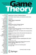
Let an instance (N, A, P, R) of ${\textsf {s{-}GASP}}$ be given. A feasible assignment is an assignment meeting the constraints in R. We will consider the following properties (see also Fig. 1). A feasible assignment $\pi$ is

• envy-free if there is no pair of agents $(i,j)\in N\times N$ with $\pi (j)\in A^{*}$ such that $\pi (j)\succ _{i}\pi (i)$ holds (i.e., no agent prefers any activity of $A^*$ assigned to another agent to her own activity);

• individually rational if for each $i\in N$ we have $\pi (i)\succsim _{i} a_{\emptyset }$ (i.e., every agent ends up with an activity that is acceptable for her);

• individually stable if there is no agent i and no activity $a\in A$ such that (1) $a\succ _{i}\pi (i)$ and (2) the mapping $\pi '$ defined by $\pi '(i)=a$ and $\pi '(k)=\pi (k)$ for $k\in N\setminus \{i\}$ is a feasible assignment (i.e., no agent can switch to a preferred activity without violating the constraints);

• core stable if there is no pair (E, a) where $E\subseteq N$ and $a\in A$ such that (1) $a\succ _{i}\pi (i)$ for all $i\in E$, (2) $\pi ^{a}\subset E$ holds if $a\in A^{*}$, and (3) the mapping $\pi '$ defined by $\pi '(i)=a$ for $i\in E$ and $\pi '(k)=\pi (k)$ for $k\in N\setminus E$ is a feasible assignment (i.e., no set of agents can reorganize itself in a way that each of them receives a more preferred activity and no constraint is violated); (Note that the respective activity a to which the set E of agents wishes to deviate must be either $a_{\emptyset }$ or currently unused because the agents in a non-empty set $\pi ^a$, $a \in A^*$, are not better off by agents joining as their preferences only depend on the activities.)

• strictly core stable if there is no pair (E, a) where $E\subseteq N$ and $a\in A$ such that (1) $a\succsim _{i}\pi (i)$ for all $i\in E$ where $a\succ _{i}\pi (i)$ for at least one $i\in E$, (2) $\pi ^{a}\subset E$ holds if $a\in A^{*}$, and (3) the mapping $\pi '$ defined by $\pi '(i)=a$ for all $i\in E$ and $\pi '(k)=\pi (k)$ for $k\in N\setminus E$ is a feasible assignment (i.e., no set of agents can reorganize itself in a way that some of them receive a more preferred activity whereas the remaining agents do not change for the worse, and no constraint is violated);

• Pareto optimal if there is no feasible assignment $\pi '$ that Pareto-dominates $\pi$: that is, if there is no feasible assignment $\pi '\not =\pi$ such that $\pi '(i)\succsim _{i}\pi (i)$ for all $i\in N$ and $\pi '(i)\succ _{i}\pi (i)$ for at least one $i\in N$ (i.e., the whole group of agents cannot reorganize in a way that some agents receive a more preferred activity whereas the remaining agents do not change for the worse, and no constraint is violated).

Requirement $E\supset \pi ^a$ in the definition of (strict) core stability follows the idea that agents cannot be removed from their assigned activity. Observe that, with the set of constraints R considered in this paper, a main difference between the concepts of (strict) core stability and individual stability is based on the size constraints for the activities.

Most of the above solution concepts are typically considered to assess the quality of an assignment in problems from matching theory and, in particular, hedonic games²—depending on the particular setting, it makes more sense to consider one or the other of them. Since simplified group activity selection has a certain vicinity to both of the problems, we translated them to our setting and consider this whole variety of criteria.

Remark 1

Another common notion of stability is Nash stability. In the hedonic games framework, the difference between Nash stability and individual stability is that the latter refers to deviations in which all members of a coalition C welcome the agent that wishes to join C. In contrast to hedonic games, in the setting of s-GASP the agents do not have preferences over other agents. Therefore, in s-GASP the solution concepts of Nash stability and individual stability coincide.

We begin with a short example highlighting some of the above solution concepts.

Example 1

Let $N=\{1,2,3,4\}$ and $A^{*}=\{a,b\}$, with $\ell (a)=1$, $\ell (b)=2$, and $u(a)=u(b)=4$. The agents’ preferences are given as follows:

$$\begin{aligned}{ \begin{array}{cc} \succsim _1 :\, &{} \mathbf {a} \succ _1 b \succ _1 a_{\emptyset }\\ \succsim _2 :\, &{} a \succ _2 \mathbf {b} \succ _2 a_{\emptyset }\\ \succsim _3 :\, &{} \mathbf {b} \succ _3 a \succ _3 a_{\emptyset }\\ \succsim _4 :\, &{} \mathbf {b} \succ _4 a \succ _4 a_{\emptyset }\\ \end{array}} \end{aligned}$$

Consider the assignment $\pi$ with $\pi (1)=a$ and $\pi (2)=\pi (3)=\pi (4)=b$; in particular, we have $\pi ^{a}=\{1\}$. (The activity assigned to each agent by $\pi$ is printed in bold in each agent’s preference order above.) The assignment $\pi$ is individually rational because there is no agent i who prefers $a_{\emptyset }$ over $\pi (i)$. However, $\pi$ is not envy-free since agent 2 envies agent 1 for activity a. In addition, it turns out that $\pi$ is not individually stable, because agent 2 wants to deviate to a with the resulting assignment $\pi '$ given by $\pi '(1)=\pi '(2)=a$ and $\pi '(3)=\pi '(4)=b$ being feasible. Similarly, $\pi$ is not strictly core stable since in the coalition $E=\{1,2\} \supset \pi ^a$, agent 2 can be made better off by making her join a, while agent 1 does not change for the worse. On the other hand, $\pi$ is core stable: the only possible coalition E making each of its members strictly better off would be $E=\{2\}$ with a deviation towards a, but the transition to activity a is not permitted as a is neither the void activity nor unused under $\pi$. Finally, in contrast to $\pi '$, assignment $\pi$ is not Pareto optimal.

Stability of a solution can have several reasons: the agents are all happy with the assignment and do not want to change it; or they are not as happy as they could be, but they cannot deviate because of the constraints.³ The constraints might be violated in different ways. For the class of constraints we consider, an alternative notion of stability, namely the notion of virtual stability, is interesting. Both types of stability notions incorporate the condition that agents cannot be simply removed from assigned activities. However, in contrast to the above defined stability notions in which a deviation requires the feasibility of the resulting assignment, virtual stability captures the idea that a deviating (group of) agent(s) is only concerned with the “feasibility” with respect to the activity the (group of) agent(s) wants to join, irrespective of whether or not the size constraints of the left activities are met: it thus requires that a deviation from the assigned activity towards a more preferred activity a violates the capacity constraints of a.

Formally, we define the following stability concepts (for the sake of conciseness we set $\ell (a_{\emptyset })=1$ and $u(a_{\emptyset })=n$).

A feasible assignment $\pi$ is

• virtually individually stable if there is no agent i and no activity $a\in A$ with $\ell (a)\le |\pi ^{a}|+1\le u(a)$ such that $a\succ _{i}\pi (i)$ holds;

• virtually core stable if there is no pair (E, a) where $E\subseteq N$ and $a\in A$ with $\ell (a)\le |E|\le u(a)$ such that (i) $a\succ _{i}\pi (i)$ for all $i\in E$, and (ii) $\pi ^{a}\subset E$ holds if $a\in A^{*}$;

• virtually strictly core stable if there is no pair (E, a) where $E\subseteq N$ and $a\in A$ with $\ell (a)\le |E|\le u(a)$ such that (i) $a\succsim _{i}\pi (i)$ for all $i\in E$ where $a\succ _{i}\pi (i)$ for at least one $i\in E$, and (ii) $\pi ^{a}\subset E$ holds if $a\in A^{*}$.

Note that as in the definition of core stability, also in virtual core stability the respective activity a to which the set E of agents wishes to deviate must be either the void activity $a_{\emptyset }$ or currently unused. The following example indicates the difference between stability and virtual stability, which lies in the fact that the latter notion refers to deviations which do not take into account the level of lower bounds on the activities that are left; in the example, this is illustrated by means of the respective notions of (virtual) individual stability.

Example 2

Let $N=\{1,2,3\}$, $A^{*}=\{a,b\}$ with $\ell (a)=1$, $u(a)=2$ and $\ell (b)=2=u(b)$, with the following preference profile:

$$\begin{aligned}{ \begin{array}{cc} \succsim _1 :\, &{} \mathbf {a} \succ _1 b \succ _1 a_{\emptyset }\\ \succsim _2 :\, &{} a \succ _2 \mathbf {b} \succ _2 a_{\emptyset }\\ \succsim _3 :\, &{} \mathbf {b} \succ _3 a \succ _3 a_{\emptyset }\\ \end{array}} \end{aligned}$$

Assignment $\pi$ with $\pi (1)=a$ and $\pi (2)=\pi (3)=b$ is individually stable (and also individually rational), because due to the lower bound of 2 on activity b, agent 2 cannot deviate towards a without violating feasibility. On the other hand, $\pi$ is not virtually individually stable, because a deviation of agent 2 towards activity a meets the capacity bounds of a since $u(a)=2$ and $\pi$ assigns only one agent to a.

Finally, an individually rational assignment $\pi$ is maximum individually rational if for all individually rational assignments $\pi '$ we have $\#(\pi )\ge \#(\pi ')$.

Fig. 1

Relations between the solution concepts we consider. An arrow directed from A to B means A implies B; e.g., a Pareto optimal assignment is also strictly core stable. For the solution concepts in bold a respective assignment always exists (see also Sect. 3)

The relationships between the solution concepts are shown in Fig. 1. Notably for none of the relations the converse holds as well. As the below Theorem 1 shows, the technical subtleties of the solution concepts lead to some surprising results. This also fixes an error in the corresponding figure in our previous work (Darmann et al. 2017) where we erroneously claimed that (virtual) core stability implies (virtual) individual stability.

Before turning to Theorem 1, however, we briefly provide the key arguments for the relations between the solution concepts depicted in Fig. 1:

• virtually strictly core stable $\Rightarrow$ virtually individually stable. This follows directly from the definition of a virtually strictly core stable assignment by setting $E=\{i\}$.

• virtually strictly core stable $\Rightarrow$ virtually core stable. Consider a feasible assignment $\pi$ and some pair (E, a) with $E\subseteq N$ and $a \in A$. If $a\succsim _i \pi (i)$ does not hold for all members of E, then $a\succ _i \pi (i)$ does not hold for all members of E. Therewith, the statement follows.

• virtually strictly core stable $\Rightarrow$ strictly core stable. This follows from the fact that, if the size constraints of the activity a which the group of agents wants to join is not met, then the resulting assignment cannot be feasible.

• Pareto optimal $\Rightarrow$ strictly core stable. Assume a feasible assignment $\pi$ is not strictly core stable. Then a group E of agents can deviate towards an activity a in a way that (1) makes at least one member of E better off without making one member of E worse off, and (2) results in a feasible assignment $\pi '$. Thus, $\pi '$ Pareto-dominates $\pi$, which proves our statement.

• virtually individually stable $\Rightarrow$ individually stable. This follows from the fact that, if the size constraints on the activity a towards which the agent wants to deviate is not met, then the resulting assignment is not feasible.

• virtually individually stable $\Rightarrow$ individually rational. An assignment that is virtually individually stable is necessarily also individually rational, because an agent assigned to an activity she prefers $a_{\emptyset }$ to can trivially deviate towards $a_{\emptyset }$ without violating its size constraints, as there are no constraints on $a_{\emptyset }$.

• virtually core stable $\Rightarrow$ individually rational. Analogously to the above, a group of agents E in which all of its members are better off by deviating to $a_{\emptyset }$ can trivially deviate towards $a_{\emptyset }$ without violating its size constraints, as there are no constraints on $a_{\emptyset }$.

• virtually core stable $\Rightarrow$ core stable. This follows analogously to (virtually strictly core stable $\Rightarrow$ strictly core stable).

• strictly core stable $\Rightarrow$ core stable. This follows analogously to (virtually strictly core stable $\Rightarrow$ virtually core stable).

Theorem 1

There are instances of s-GASP with assignments which are

• 1. (virtually) core stable but neither (virtually) individually stable nor (virtually) strictly core stable,

• 2. virtually strictly core stable but not Pareto optimal,

• 3. Pareto optimal but not individually rational

• 4. individually stable but not individually rational,

• 5. individually stable and individually rational but not virtually individually stable.

Proof

Statement 1 follows from Example 1, Statement 5 from Example 2. The Statements 2–4 hold as a consequence of the two examples below. In particular, the Example 3 below proves Statement 2. Example 4 given below shows Statement 3 and Statement 4. $\square$

Example 3

Let $N=\{1,2\}$, $A^{*}=\{a,b\}$ with $\ell (x)=1=u(x)$ for all $x \in A^*$. Consider the following preference profile:

$$\begin{aligned} { \begin{array}{cc} \succsim _1 :\, &{} a \succ _1 \mathbf {b} \succ _1 a_{\emptyset }\\ \succsim _2 :\, &{} b \succ _2 \mathbf {a} \succ _2 a_{\emptyset }\\ \end{array}} \end{aligned}$$

Then, the assignment $\pi$ with $\pi (1)=b$ and $\pi (2)=a$ is virtually strictly core stable but not Pareto optimal.

Example 4

Let $N=\{1,2\}$, $A^{*}=\{a,b\}$ with $\ell (x)=2=u(x)$ for all $x \in A^*$, and the following preference profile:

$$\begin{aligned} { \begin{array}{cc} \succsim _1 :\, &{} \mathbf {a} \succ _1 a_{\emptyset }\succ _1 b \\ \succsim _2 :\, &{} b \succ _2 a_{\emptyset }\succ _2 \mathbf {a} \\ \end{array}} \end{aligned}$$

Assignment $\pi$ with $\pi (1)=\pi (2)=a$ is Pareto optimal and individually stable (agent 2 cannot deviate to $a_{\emptyset }$ without violating the constraints of activity a), but neither individually rational nor virtually individually stable (there are no constraints on $a_{\emptyset }$, hence a deviation of agent 2 towards $a_{\emptyset }$ trivially satisfies the constraints on $a_{\emptyset }$). Hence, $\pi$ is also not virtually strictly core stable.

We point out that for the special case of $\ell (a)=1$ for each activity $a\in A^{*}$, virtual (strict) core stability coincides with (strict) core stability, and virtual individual stability coincides with individual stability. In addition, in this case all of the considered solution concepts except envy-freeness imply individual rationality; the latter is a consequence of the below proposition and the relations between the solution concepts displayed in Fig. 1.

Proposition 1

In s-GASP, if for each activity $a\in A^{*}$ we have $\ell (a)=1$, then any assignment that is core stable or individually stable is individually rational.

Proof

In the case $\ell (a)=1$ for all $a\in A^{*}$, consider an assignment $\pi$ which is not individually rational. Then there must be an agent i who is assigned to some activity a she has ranked below $a_{\emptyset }$ and hence would prefer to deviate to $a_{\emptyset }$. By $\ell (a)=1$, the assignment $\pi '$ with $\pi '(i)=a_{\emptyset }$ and $\pi '(j)=\pi (j)$ for $j\in N\setminus \{i\}$ is feasible. Hence, $\pi$ is neither individually stable nor core stable. $\square$

Before we move on to the next sections where we present our complexity results, we conclude this section with the definition of the NP-complete problem Exact Cover by 3-Sets (X3C) which is used in most of the reductions in this paper. The input of an instance of X3C consists of a pair $\langle X,\mathcal{Z}\rangle$, where $X=\{1,\ldots ,3q\}$ and $\mathcal{Z}=\{Z_{1},\ldots ,Z_{p}\}$ is a collection of 3-element subsets of X; the question is whether we can cover X with exactly q sets of $\mathcal{Z}$. Throughout the paper, we assume that each element of X is contained in exactly three sets of $\mathcal{Z}$; this implies that $p=3q$ holds. X3C is known to be NP-complete in this case (Gonzalez 1985). For each $i\in X$, we will always denote the sets containing i by $Z_{i_{1}},Z_{i_{2}},Z_{i_{3}}$ with $i_{1}<i_{2}<i_{3}$.

3 Computing “good” assignments

We will now consider the computational complexity of ${\textsf {s{-}GASP}}$ for the various solution concepts presented in the previous section. An overview of our results is given in Table 1. For each of the considered solution concepts, we first deal with the question of finding assignments with the desired properties or verifying them; then, we turn to an optimization variant.

Table 1 Overview of complexity results obtained for constraints $|\pi ^{a}|\in \{0\}\cup [\ell (a),u(a)]$, $a\in A^{*}$.

Naturally, the first interesting question is whether “good” assignments exist and how to find them. In this section, we either provide hardness results for the first question (implying hardness of finding a respective assignment) or we provide a polynomial-time algorithm for finding a respective assignment (except for Pareto optimal assignments, which always exist but in general turn out to be computationally hard to determine). For each of the considered concepts, we then turn to an optimization problem: among all feasible assignments that feature a certain property, one is usually interested in finding one that maximizes the number of agents that are assigned to a non-void activity, thus keeping the number of agents who cannot be enrolled in any activity low. The decision version of this problem asks the question whether, for some given k, at least k agents can be assigned to non-void activities. In this section, we either provide a polynomial-time algorithm that determines a “good” assignment maximizing the number of agents assigned to non-void activities (implying that the corresponding decision problem is in P), or provide hardness results for the above stated decision problem (which in turn implies hardness of finding a corresponding assignment).

This section is structured as follows. We begin with the two most basic concepts of feasibility and individual rationality in Sect. 3.1. Section 3.2 is dedicated to Pareto optimal assignments. Then, we consider the stability notions⁴ of (virtual) individual stability, (virtual) core stability, and (virtual) strict core stability in Sect. 3.3. We conclude the section with envy-free assignments in Sect. 3.4.

3.1 Feasible and individually rational assignments

Obviously, assigning the void activity to every agent results in a feasible, individually rational and also envy-free assignment. In addition, it can be checked in polynomial time whether a given assignment is feasible or individually rational.

The task of maximizing the number of agents assigned to a non-void activity in a feasible or individually rational assignment, however, is more challenging. On the positive side, if we are only interested in a feasible assignment maximizing the number of agents assigned to a non-void activity, we can find such an assignment in polynomial time.

Proposition 2

In s-GASP, in polynomial time we can find a feasible assignment that maximizes the number of agents assigned to a non-void activity.

Proof

We need to find the maximum number $k\le n$ such that taking, for each $a\in A^*$, exactly one number of $\{0\}\cup [\ell (a),u(a)]$, adds up to k. This problem corresponds to the Multiple-Choice Subset-Sum problem (Pisinger 1995); in our case, the latter allows for an overall polynomial-time algorithm since u(a) is bounded by n. $\square$

But already for individually rational assignments it is NP-complete to decide whether all agents can be assigned to a non-void activity (stated in Theorem 2 below). We note that Theorem 2, where we consider the decision for an assignment of all agents, is stronger than the result implied by Arulselvan et al. (2018, Theorem 1), namely that the decision problem whether it is possible to assign $\ge k$ agents to non-void activities such that the assignment is individually rational is NP-complete.

Theorem 2

It is NP-complete to decide whether s-GASP admits an individually rational assignment that assigns each agent to some $a\in A^{*}$, even when each agent has strict preferences and for each activity $a\in A^{*}$ we have $\ell (a)=3$ and $u(a)=n$.

Proof

This is shown by a reduction from Exact Cover by 3-Sets (see Appendix). $\square$

However, if we have $\ell (a)=1$ for each $a \in A^*$, then we can find a maximum individually rational assignment—i.e., an individually rational assignment which maximizes the number of agents assigned to a non-void activity—efficiently, since it is straightforward to translate this task to a (many-to-one) simple b-matching problem, which can be solved in polynomial time (see, e.g., the textbook by Korte and Vygen 2012, Chapter 12). In a simple b-matching problem, we are given an undirected graph $G=(V,E)$ and a mapping $b:V\rightarrow \mathbb {N}_0$; a b-matching is a subset $T\subseteq E$ such that for each vertex v there are at most b(v) edges in T that have v as an endpoint; the goal is to find a b-matching of maximum cardinality. In this kind of matching problems, the vertices of an undirected graph come with a bound b on the number of vertices they can be matched with (the case $b=1$ for all vertices corresponds to the ordinary matching problem).

Proposition 3

In s-GASP, if for each activity $a\in A^{*}$ we have $\ell (a)=1$, then in polynomial time we can find a maximum individually rational assignment.

3.2 Pareto optimal assignments

We now turn our attention to Pareto optimal assignments. Our first result shows that finding a Pareto optimal assignment in ${\textsf {s{-}GASP}}$ is NP-hard even for the case $u(a)=n$ for each activity a.

Theorem 3

In s-GASP, it is NP-hard to find a Pareto optimal assignment, even when for each activity $a\in A^*$ we have $\ell (a)=3$ and $u(a)=n$.

Proof

This is shown by a reduction from Exact Cover by 3-Sets (see Appendix). $\square$

However, in the case of $\ell (a)=1$ for each $a\in A^{*}$, we can even find a Pareto optimal assignment that maximizes the number of agents assigned to a non-void activity in polynomial time (see Corollary 1 at the end of Sect. 3.2).

Next, we turn to the question of verification of Pareto optimality. In particular, checking whether a given assignment is Pareto optimal is coNP-complete as the following theorem shows.

Theorem 4

In s-GASP, it is coNP-complete to decide if a given assignment is Pareto optimal, even when each agent has strict preferences and for each activity $a\in A^{*}$ we have $u(a)=n$.

Proof

This is shown by a reduction from Exact Cover by 3-Sets (see Appendix). $\square$

We remark that if there are no restrictions on the minimum number of participants of each activity, the latter problem can be modeled as a minimum cost flow problem and hence becomes tractable.

Theorem 5

In s-GASP, if for each activity $a\in A^{*}$, we have $\ell (a)=1$, then in polynomial time we can decide if a given assignment is Pareto optimal.

Proof

Given instance $\mathcal {I}=(N,A,P,R)$ of ${\textsf {s{-}GASP}}$ with $\ell (a)=1$ for all $a\in A^{*}$ and assignment $\pi$, we construct instance $\mathcal {C}$ of the minimum cost flow problem with lower bounds (see, e.g., Ahuja et al. 1993, Chapter 2.4). Note that $\pi$ must be individually rational. In instance $\mathcal {C}$, the directed graph $G=(V,E)$ along with edge costs, lower bounds (i.e., the minimum amount that must flow on an edge) and capacities (i.e., the maximum amount that can flow on an edge) of the edges are given as follows (see also Fig. 2 for an illustration). $G=(V,E)$ has vertex set $V=\{s,t\}\cup N\cup A^{*}$, the edge set E consists of the following edges:

Fig. 2

Illustration of the construction of a flow instance in the proof of Theorem 5. Consider instance $\mathcal {I}$ of s-GASP with $N=\{1,2,3\}$ and $A^*=\{a,b,c\}$, where $u(a)= 1$, $u(b)= 3$, and $u(c)=2$. The agents’ preferences are given by $a \succ _{1} b \succsim _1 c \succ _1 a_{\emptyset }$, $b\succ _2 c \succ _2 a \succ _2 a_{\emptyset }$, and $c \succ _3 a_{\emptyset }\succ _3 b \succsim _3 a$. The graph in the figure refers to assignment $\pi$ with $\pi (1)=\pi (2)=c$ and $\pi (3)=a_{\emptyset }$; lower bound and capacity of an edge are displayed in brackets, the costs are displayed in italic. Assignment $\pi$ is not Pareto optimal, because there is a flow of negative total cost in the graph. For instance, the flow (displayed in bold) that sends one unit along each of the edges (s, 1), (1, a), (a, t), (s, 2), (2, c), (s, 3), (3, c) and two units along (c, t) induces a feasible assignment $\pi '$ with $\pi '(1)=a$ and $\pi '(2)=\pi '(3)=c$, which Pareto-dominates $\pi$

• for $i\in N$, edge (s, i) of zero cost, and, for $a\in A^{*}$ with $a\succsim _{i}\pi (i)$, edge (i, a) of cost $-1$ if $a\succ _{i}\pi (i)$ and of cost 0 if $a\sim _{i}\pi (i)$

• for $a\in A^{*}$ edge (a, t) of capacity u(a)

Both lower bound and capacity of edge (s, i) are equal to 1 iff $\pi (i)\succ _ia_{\emptyset }$ holds. Unless otherwise specified above, the lower bound of edge $e\in E$ is 0, its capacity is 1, and its cost is 0.

Assume there is an integer flow f of negative total cost. Consider the assignment $\pi '$ defined by $\pi '(i)=a$ iff f sends flow through edge (i, a). Then, by construction we must have $\pi '(i)\sim _i \pi (i)$ or $\pi '(i)\succ _{i}\pi (i)$ for each $i\in N$, where the latter holds for at least one agent $i\in N$ by the negative total cost of f. Thus, $\pi$ is not Pareto optimal.

If, on the other hand, $\pi$ is not Pareto optimal, then there is an assignment $\pi '$ with $\pi '(i)\sim _i \pi (i)$ or $\pi '(i)\succ _{i}\pi (i)$ for each $i\in N$, where the latter holds for at least one $i\in N$. The integer flow $f'$ that, for each $i \in N$ and $a \in A$ with $\pi '(i)=a$, sends one unit along the edges (s, i), (i, a), (a, t) has negative total cost.

Therewith, for verifying if $\pi$ is Pareto optimal it is sufficient to find an integer minimum cost flow in instance $\mathcal {C}$. Under the use of a standard transformation to remove non-zero lower bounds (see Ahuja et al. 1993, Chapter 2.4), such an integer minimum cost flow can be determined in polynomial time by applying, e.g., a network simplex algorithm (see Ahuja et al. 1993, Chapter 11); for instance, with $|V|\in \mathcal {O}(n+m)$, $|E|\in \mathcal {O}(m+n+mn)$ and maximum cardinality edge cost of 1, the algorithm of Tarjan (1997) runs in $\mathcal {O}((n+m)(m+n+mn)(\log (n+m))^2)$ and hence in $\mathcal {O}((m^2n+mn^2)(\log (n+m))^2)$ time. $\square$

In the remainder of Sect. 3.2, we consider the computational complexity involved in maximizing the number of agents assigned to non-void activities in Pareto optimal assignments. In the framework of course allocation, if all agents have strict preferences, it is known that a Pareto optimal matching—that assigns an agent to an activity (course) only if the activity is acceptable for the agent—can be found in polynomial time (Cechlárová and Fleiner (2017); Kamiyama (2013)). Since in our setting (1) the agents’ preferences are represented by weak orders and (2) Pareto optimality does not require individual rationality, these results do not immediately translate. For the latter reason, the computational intractability result by  Cechlárová and Fleiner (2017) (for finding a Pareto optimal matching maximizing the number of agents assigned to a non-void activity if each agent can be assigned to at most one activity) does not immediately translate to our setting either.

By Theorem 3 we know that finding a Pareto optimal assignment that maximizes the number of agents assigned to non-void activities is NP-hard even for the case $u(a)=n$ for each activity a.

The general problem of deciding if there exists a Pareto optimal assignment that assigns each agent to a non-void activity turns out to be computationally hard.

Theorem 6

It is NP-hard to decide whether s-GASP admits a Pareto optimal assignment that assigns each agent to a non-void activity.

Proof

This is shown by a reduction from Exact Cover by 3-Sets (see Appendix). $\square$

However, as the following theorem shows, if we relax the constraints on the lower bound of the group sizes, the problem becomes computationally tractable.

Theorem 7

In s-GASP, if for each activity $a\in A^{*}$ we have $\ell (a)=1$ then in polynomial time we can find a Pareto optimal assignment that maximizes the number of agents assigned to a non-void activity.

Proof

Recall that in the case $\ell (a)=1$ for all $a\in A^{*}$ a Pareto optimal assignment is also individually rational (see Proposition 1 and Fig. 1). Let k be the maximum number of agents assigned to non-void activities by an individually rational assignment (recall that, due to Proposition 3, such an assignment can be found in polynomial time). Hence, it is sufficient to find a Pareto optimal assignment $\pi$ with $\#(\pi )=k$.

Given an instance $\mathcal {I}=(N,A,P,R)$ of ${\textsf {s{-}GASP}}$ with $\ell (a)=1$ for all $a\in A^{*}$, we construct an instance $\mathcal {F}$ of the min cost flow problem with directed graph $G=(V,E)$. Set ${V=\{s,t\}\cup N\cup A^{*}}$, and let the edges and their capacities be given as follows: for each $i\in N$, introduce edge (s, i) with capacity 1; for each $a\in A^{*}$ and $i\in N$ introduce an edge (i, a) of capacity 1 if $a\succsim _{i}a_{\emptyset }$ holds; for each $a\in A^{*}$, introduce edge (a, t) of capacity u(a).

We introduce non-zero costs on some edges of the graph: for each $a\in A^{*}$ and $i\in N$, edge (i, a) has cost $-(1+|\{b\in A^{*}\mid a\succ _{i}b,\,b\succ _{i}a_{\emptyset }\}|)$ if $a\succ _i a_{\emptyset }$ and cost 0 if $a\sim _i a_{\emptyset }$; all remaining edges have zero cost.

Observe that there is a one-to-one correspondence between a feasible assignment $\pi$ with $\#(\pi )=k$ and a (feasible) flow of size k. First, given $\pi$, sending a unit of flow along the sequence of edges (path) (s, i), (i, a), (a, t) iff i is assigned to activity a yields a flow of size k from s to t meeting all the edge capacity constraints. Second, a flow of size k from s to t must send a total of k units through edges (i, a) with $i \in N$ and $a \in A^{*}$ such that at most one unit is sent through (s, i) for any $i \in N$; since the capacity constraints of the edges (a, t) correspond to u(a) for $a \in A^{*}$, the assignment $\pi$ defined by setting $\pi (i)=a$ iff f sends a unit of flow through edge (i, a) is feasible.

Now, let f be a minimum integer cost flow of size k in instance $\mathcal {F}$. Then f induces the assignment $\pi$ by setting $\pi (i)=a$ iff f sends a unit of flow through edge (i, a). Assignment $\pi$ is Pareto optimal since otherwise a flow $f'$ of lower total cost than the total cost of f could be induced. $\square$

Recall that due to Proposition 1 in the case $\ell (a)=1$ for each $a\in A^{*}$, also any strictly core stable, core stable, or individually stable assignment is individually rational. In addition, in this case virtual (strict) core stability coincides with (strict) core stability, and virtual individual stability coincides with individual stability. Hence we can state the following corollary.

Corollary 1

In s-GASP, if for each activity $a\in A^{*}$ we have $\ell (a)=1$, then in polynomial time we can find a maximum individually rational assignment that is Pareto optimal, (virtually) individually stable, (virtually) core stable and (virtually) strictly core stable.

3.3 Stable assignments

The good news is that for several stability concepts, a corresponding assignment always exists and can efficiently be found, as, for instance, the following theorem shows.

Theorem 8

In s-GASP, a strictly core stable assignment always exists and can be found in polynomial time.

Proof

We present in Algorithm 1 a polynomial-time algorithm for finding a strictly core stable assignment.

Outline The basic idea behind Algorithm 1 is as follows. Starting with a feasible assignment $\pi$, for each agent i and each activity b which i prefers to $a=\pi (i)$, we check whether there is a subset of agents including agent i that want to deviate to b such that the resulting assignment is feasible. That is, we check whether there is a set of agents $E\supset \pi ^{b}$ such that (1) for all $j\in E$ we have that $b\succsim _{j}\pi (j)$ holds (recall that for agent i it holds that $b\succ _{i}\pi (i)$) and (2) $\pi '$ with $\pi '(i)=b$ for $i\in E$ and $\pi '(j)=\pi (j)$ for $j\in N\setminus E$ is a feasible assignment. In order to do so, we store all activities agent i prefers over $a=\pi (i)$ into set D (lines 5-6). While D is non-empty (line 7), we take an activity $b \in D$ and compute the set of agents B which are not worse off by deviating to b (lines 8-9). Then, for each activity $c\in A\setminus \{b\}$, we compute the possible numbers of agents in the set $\pi ^{c}$ that agree with joining b and can be removed from $\pi ^{c}$ while still enabling a feasible assignment—these numbers are stored in the set $R^{c}$ (lines $10-17$). Note that 0 must be removed from $R^{a}$ since we need to include agent i (line 18). Given these numbers, we then verify if—including i and the agents in $\pi ^{b}$—these add up to an integer contained in $[\ell (b),u(b)]$ by taking exactly one number from each activity (note that for activity b we need to include the whole amount $|\pi ^b|$ of agents assigned to b under $\pi$; line 20). If this is the case we can assign a subset of agents including $\{i\}\cup \pi ^b$ to B, and we update our assignment accordingly (lines $21-29$). Finally, we update D to the set of activities different from b that agent i prefers over the activity she is currently assigned to (line 30).

Termination and correctness Each for-loop in the algorithm iterates over at most $\max \{m,n\}$ elements. For the inner while-loop starting in line 7 (“while $D\not =\emptyset$”), note that the last line of the loop (line 30) implies that the set D in the statement of the loop is updated to a proper subset of itself. Next, observe that during execution of the algorithm, an agent either remains assigned to the originally assigned activity, say a, or is assigned to some activity that does not make her worse off than a (in lines 21, 22, 24 or 26); in addition, whenever some agent is assigned to a new activity, at least one agent is better off than before. Hence, at most mn times some agents can be assigned to a new activity. Now, for the outer while-loop starting in line 3 (“while $N\setminus N'\not =\emptyset$”), consider lines 32–35. If agent i is not assigned to a new activity, the set $N'$ is augmented by the singleton set $\{i\}$ in line 33. If she is assigned to a new activity, $N'$ is set to the empty set in line 35, and the loop in line 3 (“while $N\setminus N'\not =\emptyset$”) re-starts with the whole set $N\setminus N'=N$. However, at the end of the loop, we either augment the set $N'$ or set $N'=\emptyset$, and the latter can happen at most mn times. Thus, the algorithm terminates. For correctness, observe that the algorithm terminates when each agent i is contained in $N'$. By construction, the algorithm sets $N'=\emptyset$ whenever it is possible to assign some agent i to an activity b with $b\succ _i \pi (i)$, such that for some set $E\supset \pi ^b$ it holds that (1) each agent $j \in E\setminus \{i\}$ is not worse off with a deviation towards b, and (2) the resulting assignment is feasible. Therefore, the assignment $\pi$ which is finally determined by the algorithm is strictly core stable.

Running time As far as the running time of Algorithm 1 is concerned, its bottleneck is to decide whether we can add up the above-mentioned numbers to be in the interval $[\ell (b),u(b)]$. That problem reduces to the Multiple-Choice Subset-Sum problem (Pisinger 1995), which can be stated as follows: Given k classes $N_1, \ldots , N_k$, each class $N_i$ containing non-negative integer weights $w_{1i}, \ldots , w_{n_i i}$, and a capacity bound c, we ask whether we can select exactly one element from each class such that the total weight sum adds up to c. For our problem, the weights in class $N_i$ correspond to the possible numbers of agents in the set $R^{a_i}$ for activity $a_i$. We can now apply Pisinger’s algorithm (Pisinger 1995)⁵, which has a complexity in $\mathcal {O}(ab)$, where a is the largest weight—hence bounded by the number n of agents in our case—and b is the number of all weights, which is bounded by $m(n+1)$ in our case since there are at most as many weights per activity as the number of agents plus 1 (for weight 0). We hence have a running time of $\mathcal {O}(mn^{2})$ per execution of line 20. For each agent, we need to execute line 20 of our algorithm at most $m\cdot mn$ times. Thus, the overall running time of Algorithm 1 can roughly be bounded by $\mathcal {O}(m^{3}n^4)$. $\square$

Recall that a strictly core stable assignment is also core stable and individually stable. Hence, as a consequence of the above theorem, also a core stable and individually stable assignment always exists and can efficiently be found. As it turns out, an analogous result holds for virtually individually stable assignments.

Theorem 9

In s-GASP, a virtually individually stable assignment always exists and can be found in polynomial time.

Proof

In an instance (N, A, P, R) of ${\textsf {s{-}GASP}}$, we initially assign each agent to $a_{\emptyset }$, i.e., set $\pi (i)=a_{\emptyset }$ for $i\in N$. For $a\in A^{*}$ with $\ell (a)\ge 2$, if no agent is assigned to such a, then $\ell (a)\le |\pi ^{a}|+1$ cannot hold. Hence, in what follows, we only consider activities $a\in A^{*}$ with $\ell (a)=1$. For $1\le i\le n$, assign agent i to the best ranked such activity $a\succ _{i}a_{\emptyset }$ with $|\pi ^{a}|<u(a)$ and update $\pi$ (i.e., set $\pi (i)=a$ while $\pi (j)$ remains unchanged for $j\in N\setminus \{i\}$). The resulting assignment $\pi$ is virtually individually stable: for each agent i, by construction, each activity a with $a\succ _{i} \pi (i)$ has (1) no agent assigned to and $\ell (a)\ge 2$—which implies that the agent alone cannot deviate to a without violating the lower bound on a—or (2) already u(a) agents assigned to, and thus the agent cannot join a without violating the upper bound on a.$\square$

In contrast, a virtually core stable (and thus a virtually strictly core stable) assignment does not always exist, as the following example shows. It corresponds to the phenomenon referred to as Condorcet’s voting paradox (Marquis de Condorcet 1785) which reappears in many settings dealing with preferences.

Example 5

Let $N=\{1,2,3\}$ and $A^{*}=\{a,b,c\}$, with $a\succ _{1}b\succ _{1}c\succ _{1}a_{\emptyset }$, $b\succ _{2}c\succ _{2}a\succ _{2}a_{\emptyset }$, and $c\succ _{3}a\succ _{3}b\succ _{3}a_{\emptyset }$. The restrictions on the activities are given by $\ell (x)=2$ and $u(x)=3$ for each $x\in A^{*}$. By the restrictions given, there is at most one non-void activity to which agents can be assigned. Clearly, for any activity $z\in A$, there is an activity $y\in A^{*}$ such that two agents prefer y to z. As a consequence, there can be no virtually core stable assignment.

In addition, the problem to decide whether or not a virtually strictly core stable assignment exists turns out to be computationally hard.

Theorem 10

It is NP-complete to decide whether s-GASP admits a virtually strictly core stable assignment, even when each agent has strict preferences and for each activity $a\in A^{*}$ we have $u(a)=n$.

Proof

For membership in NP, we check if assignment $\pi$ is virtually strictly core stable as follows. For each agent i and each activity $a\succ _{i}\pi (i)$ such that $|\pi ^{a}|<u(a)$ (otherwise, a deviation towards a would violate its capacity constraint), determine the set $E(i,a)=\{j\in N\setminus \{i\}\mid a\succsim _{j}\pi (j)\}$. Observe that $E(i,a)\supset \pi ^{a}$ holds. Now, it remains to check if $|E(i,a)\cup \{i\}|\ge \ell (a)$ holds, because then—with $\pi ^{a}<u(a)$—it follows that there is a set E with $i\in E$, $E\supset \pi ^{a}$ such that $a\succ _{i}\pi (i)$ and $a\succsim _{j}\pi (j)$ for each $j\in E$ (e.g., take set E made up of $\pi ^{a}\cup \{i\}$ together with $\max \{0,\ell (a)-|\pi ^{a}|-1\}$ agents of $E(i,a)\setminus \pi ^{a}$). Determining the set E(i, a) and checking whether $|E(i,a)\cup \{i\}|\ge \ell (a)$ holds can be done in polynomial time for each agent i and activity a, and hence we can check whether $\pi$ is virtually strictly core stable in polynomial time.

For NP-hardness we provide a reduction from Exact Cover by 3-Sets , making use of Example 5 as a gadget. Given an instance $\langle X,\mathcal{Z}\rangle$ of X3C, we define the instance $\mathcal {I}=(N,A,P,R)$ of ${\textsf {s{-}GASP}}$ as follows. Let $N=\{v_{i,1}, v_{i,2}, v_{i,3} \mid 1\le i\le p\}$ and $A^{*}=\{y_{i},a_{i},b_{i},c_{i}\mid 1\le i\le p\}$. For $1\le i\le p$, let $\ell (a_{i})=\ell (b_{i})=\ell (c_{i})=2$, and $\ell (y_{i})=9$. For each $a\in A^{*}$, let $u(a)=|N|$. For each $i\in \{1,\ldots ,p\}$, the agents $v_{i,1},v_{i,2},v_{i,3}$ represent element $i\in X$; the set $Y=\{y_1,\ldots , y_p\}$ represents the set $\mathcal {Z}$, where, for $i \in X$ and $j\in \{1,2,3\}$, we denote by $y_{i_j}$ the activity in Y that refers to the set $Z_{i_j}$. Since any virtually strictly core stable assignment is individually rational, in the profile P we omit the activities ranked below $a_{\emptyset }$; the rankings of the agents $v_{i,1},v_{i,2},v_{i,3}$ are given as follows (for the sake of readability, we omit subscripts in the rankings):

$$\begin{aligned} \begin{array}{c} v_{i,1}:\,\,y_{i_{1}}\succ y_{i_{2}}\succ y_{i_{3}}\succ a_{i}\succ b_{i}\succ c_{i}\succ a_{\emptyset }\\ v_{i,2}:\,\,y_{i_{2}}\succ y_{i_{3}}\succ y_{i_{1}}\succ b_{i}\succ c_{i}\succ a_{i}\succ a_{\emptyset }\\ v_{i,3}:\,\,y_{i_{3}}\succ y_{i_{1}}\succ y_{i_{2}}\succ c_{i}\succ a_{i}\succ b_{i}\succ a_{\emptyset }\end{array} \end{aligned}$$

Note that each set Z contains three elements, and hence each $y_{i}$, $1\le i \le p$, is preferred to $a_{\emptyset }$ by exactly 9 agents. We show that there is an exact cover in instance $\langle X,\mathcal{Z}\rangle$ if and only if there is a virtually strictly core stable assignment in instance $\mathcal {I}$.

Assume there is an exact cover C. Consider the assignment $\pi$ defined by $\pi (v_{i,h})=y_{j}$ if $i\in Z_{j}$ and $Z_{j}\in C$, for $i\in \{1, \dots , p\}$ and $h\in \{1,2,3\}$. Since C is an exact cover, assignment $\pi$ is well-defined and feasible; note that each agent is assigned to an activity she ranks first, second or third. In addition, note that for $Z_{j}\in C$, each agent that prefers $y_{j}$ to $a_{\emptyset }$ is assigned to $y_{j}$. Assume a set of agents E wishes to deviate to another activity d, such that at least one member $i\in E$ prefers d over $\pi (i)$ while there is no $j\in E$ with $\pi (j)\succ _{j}d$. By the definition of $\pi$, $d\in \{y_{i}\mid 1\le i\le p\}$ holds. Observe that $\pi ^{d}=\emptyset$ holds because C is an exact cover: for each i, exactly one of $Z_{i,1},Z_{i,2},Z_{i,3}$ is in C, and therefore to exactly one of $y_{i,1},y_{i,2},y_{i,3}$ some agents are assigned. Due to $\ell (d)=9$, it hence follows that each agent of those who prefer d to $a_{\emptyset }$ must prefer d to the assigned activity, which is impossible since, by construction of the instance, for at least one of these agents j the assigned activity is top-ranked, i.e., $\pi (j)\succ _{j}d$ holds. Therewith, $\pi$ is virtually strictly core stable.

Conversely, assume there is a virtually strictly core stable assignment $\pi$. Assume that there is an agent $v_{i,h}$ who is not assigned to one of the activities $y_{i_{1}},y_{i_{2}},y_{i_{3}}$. Then, by $\ell (y_{i})=9$ and the fact that exactly 9 agents prefer $y_{i}$ to $a_{\emptyset }$ for each $i\in \{1,\ldots ,p\}$, it follows that no agent is assigned to one of $y_{i_{1}},y_{i_{2}},y_{i_{3}}$; in particular none of $v_{i,1},v_{i,2},v_{i,3}$ is assigned to one of these activities. Analogously to Example 5 it then follows that there is no virtually strictly core stable assignment, in contradiction with our assumption.

Thus, $\pi$ assigns each agent $v_{i,h}$ to one of the activities $y_{i_{1}},y_{i_{2}},y_{i_{3}}$. For each $i\in \{1,\ldots ,p\}$, by $\ell (y_{i})=9$ and the fact that exactly 9 agents prefer $y_{i}$ to $a_{\emptyset }$ it follows that to exactly one of $y_{i_{1}},y_{i_{2}},y_{i_{3}}$ exactly 9 agents are assigned, while no agent is assigned to the remaining two activities. As a consequence, the set $C=\{Z_{i}\mid |\pi ^{y_{i}}|=9,1\le i\le p\}$ is an exact cover in instance $\langle X,\mathcal{Z}\rangle$. $\square$

As a consequence of the above theorem, we obtain the following corollary.

Corollary 2

It is NP-complete to decide whether s-GASP admits a virtually core stable assignment, even when each agent has strict preferences and for each activity $a\in A^{*}$ we have $u(a)=n$.

Proof

In the instance considered in the proof of Theorem 10, an assignment is virtually strictly core stable if and only if it is virtually core stable. More precisely, analogously to the second part of that proof, it follows that in a virtually core stable assignment for each i the following holds: to exactly one of $y_{i_{1}},y_{i_{2}},y_{i_{3}}$, exactly 9 agents are assigned, while no agent is assigned to the remaining two activities. Therewith, any group deviation would require an unused activity, and by the agents’ strict orders over their three top choices, the two solution concepts coincide. $\square$

However, recall that for the case of $\ell (a)=1$ for each $a\in A^{*}$, we get a positive complexity result (see Corollary 1 in Sect. 3.2). In particular, in this case a virtually strictly core stable assignment that maximizes the number of agents assigned to a non-void activity can be found in polynomial time.

Finally, we point out that in polynomial time we can verify whether a given assignment is stable, for each of the stability concepts considered in this section. While for (virtual) individual stability this is rather straightforward, checking for strict core stability and virtual strict core stability is less obvious: Algorithm 1 checks for the former (as a part of the algorithm) as described in the proof of Theorem 8; for the latter, we refer to the first lines of the proof of Theorem 10. Note that the respective notions of (virtual) core stability can be verified in a similar manner, with the difference that each member of the deviating group must prefer the new activity to the assigned one (and hence that activity is either $a_{\emptyset }$ or currently unused).

Let us now turn to stable assignments that maximize the number of agents assigned to non-void activities. Concerning stable assignments, we have already seen (stated in Theorem 10, Corollary 2) that it is NP-complete to decide whether a virtually (strictly, respectively) core stable assignment exists, even if the upper bound of each activity equals n. This implies hardness for the corresponding optimization problems. In contrast, recall that a strictly core stable assignment and a virtually individually stable assignment always exist (stated in Theorems 8 and 9). However, deciding whether or not there is a strictly core stable or a virtually individually stable assignment that assigns each agent to a non-void activity—and thus the corresponding optimization problem of maximizing the number of agents assigned to a non-void activity—turns out to be computationally hard even if the upper bound of each activity equals n, as we will show in the following theorems. The complexity of the optimization problem remains open for individual stability and for core stability (unless $\ell (a)=1$, for which it is solvable in polynomial time as shown by Corollary 1 in Sect. 3.2).

Theorem 11

It is NP-complete to decide whether s-GASP admits a virtually individually stable assignment that assigns each agent to some $a\in A^{*}$, even when each agent has strict preferences and for each activity $a\in A^{*}$ we have $\ell (a)=3$ and $u(a)=n$.

Proof

The proof follows analogously to the proof of Theorem 2. $\square$

In a similar manner as Theorem 2, we can prove the following theorem.

Theorem 12

It is NP-complete to decide whether s-GASP admits a strictly core stable assignment that assigns each agent to some $a\in A^{*}$, even when for each activity $a\in A^{*}$ we have $\ell (a)=3$ and $u(a)=n$.

Proof

This is shown by a reduction from Exact Cover by 3-$\textsc {Sets}$ (see Appendix). $\square$

3.4 Envy-free assignments

As already mentioned, assigning each agent to the void activity $a_{\emptyset }$ results in an envy-free assignment. In addition, in polynomial time it can be verified whether a given assignment is envy-free by simply checking, for each agent, if she prefers to the activity she is assigned to one of the activities to which some other agent is assigned. On the other hand, for envy-freeness maximizing the number of “active” agents turns again out to be hard, even in a restricted setting.

Theorem 13

It is NP-complete to decide whether s-GASP admits an envy-free assignment that assigns each agent to some $a\in A^{*}$, even when each agent has strict preferences and for each activity $a\in A^*$ we have $\ell (a)=u(a)=3$.

Proof

This is shown by a reduction from Exact Cover by 3-$\textsc {Sets}$ (see Appendix). $\square$

However, we obtain tractability for envy-freeness if we loosen the constraints on the upper bounds of the group sizes: Clearly, if there is an activity with “unlimited” capacity (i.e., its upper bound equals n), we can assign all agents to it and obtain envy-freeness. It is not clear yet whether the problem becomes tractable if $\ell (a)=1$ holds for all $a\in A^*$. This is the case though if all preference orders are strict, as the following proposition shows.

Proposition 4

In s-GASP, if all agents have strict preferences and we have $\ell (a) =1$ for all $a\in A^*$, then it can be decided in polynomial time if there exists an envy-free assignment which assigns all agents to a non-void activity.

Proof

A simple greedy algorithm can determine if there exists such an envy-free assignment. The first step is to assign each agent to her most preferred non-void activity; this meets the lower bound of each activity because of $\ell (a)=1$ for all $a\in A^*$. If the resulting (provisional) assignment $\pi$ is feasible, i.e., for all activities $a\in A^*$ the statement $u(a)\ge |\pi ^{a}|$ holds true, we are done. If this is not the case, we remove all activities a with $u(a) < |\pi ^{a}|$ from the set of activities (envy-freeness will only be accomplished if no agent is assigned to any of these activities) and start over with the first step. This algorithm either stops because all activities have been removed, or it produces an envy-free assignment which assigns all agents to a non-void activity. $\square$

4 Envy-freeness versus Pareto optimality

In many social choice settings, there is a tension between envy-freeness and Pareto optimality. This is also the case for our simplified group activity selection problem, as the following propositions show.

Proposition 5

For any $n\ge 2$, there is an instance (N, A, P, R) of ${\textsf {s{-}GASP}}$ with $\ell (a)=1$ for each $a\in A^{*}$, for which there does not exist an assignment $\pi$ which is both Pareto optimal and envy-free.

Proof

We provide a proof for $n=2$, which easily extends to $n>2$. Consider the instance with $N=\{1,2\}$, $A^{*}=\{a\}$, with the rankings $a\succ _{1}a_{\emptyset }$ and $a\succ _{2}a_{\emptyset }$, and the restrictions given by $\ell (a)=u(a)=1$. Any Pareto optimal assignment assigns exactly one agent to a, which is clearly not envy-free. $\square$

Interestingly, this tension also holds if the only relevant constraint is the lower bound of the activities (i.e., $u(a)=n$ for all a).

Proposition 6

For any $n\ge 6$, there is an instance (N, A, P, R) of ${\textsf {s{-}GASP}}$ with $u(a)=n$ for each $a\in A^{*}$, for which there does not exist an assignment $\pi$ which is both Pareto optimal and envy-free.

Proof

We provide the proof for $n=6$, which easily extends to $n > 6$. Consider the instance of ${\textsf {s{-}GASP}}$ with $N=\{1,2,3,4,5,6\},A^{*}=\{a,b,c\}$ and for each $x \in A^{*}$ we have $\ell (x)=3, u(x)=6$. The rankings are

$$\begin{aligned} \begin{array}{ccccc} \succsim _1 :\, &{} a \succ _1 b \succ _1 c \succ _1 a_{\emptyset }&{} &{} \succsim _4 :\, &{} a \succ _4 b \succ _4 c \succ _4 a_{\emptyset }\\ \succsim _2 :\, &{} b \succ _2 c \succ _2 a \succ _2 a_{\emptyset }&{} &{} \succsim _5 :\, &{} b \succ _5 c \succ _5 a \succ _5 a_{\emptyset }\\ \succsim _3 :\, &{} c \succ _3 a \succ _3 b \succ _3 a_{\emptyset }&{} &{} \succsim _6 :\, &{} c \succ _6 a \succ _6 b \succ _6 a_{\emptyset }\\ \end{array}. \end{aligned}$$

Due to the feasibility constraints, there are only 4 types of feasible assignments:

(i):

between three and five agents are assigned to the same activity $x\ne a_{\emptyset }$, and the rest to $a_{\emptyset }$;

(ii):

all agents are assigned to the void activity;

(iii):

all agents are assigned to the same activity $x\ne a_{\emptyset }$;

(iv):

three agents are assigned to the same activity $x\ne a_{\emptyset }$ and the other three agents are assigned to another activity $y\notin \{x,a_{\emptyset }\}$.

Observe that the assignments of type (i) and (ii) are Pareto-dominated by some assignment of type (iii). To verify this, consider an assignment of type (i) first. If it assigns exactly three, four or five agents to some activity, say a, and the rest to $a_{\emptyset }$, then this assignment is Pareto-dominated by the assignment that assigns all agents to a, because the agents previously assigned to $a_{\emptyset }$ are made better off. Next, consider the only assignment of type (ii), i.e., the assignment that assigns all agents to $a_{\emptyset }$. That assignment is Pareto-dominated by any assignment of type (iii) since the latter would make all agents better off.

However, an assignment $\pi _1$ of type (iii) is envy-free but not Pareto optimal. Due to the symmetrical construction of the preferences profiles, we can assume without loss of generality $\pi _{1}(i)=a$ for all $i \in N$. But then the assignment is Pareto-dominated by the assignment $\pi _2$ with $\pi _{2}(1)=\pi _{2}(3)=\pi _{2}(4)=a$ and $\pi _2(2)=\pi _{2}(5)=\pi _{2}(6)=c$. Finally, an assignment of type (iv) cannot be envy-free. Without loss of generality, we can assume $x=a$ and $y=b$, because by construction the pair (a, b) is symmetric to all other pairs. Assume, for the sake of contradiction, that there is such an envy-free assignment. Agents 1 and 4 must then be assigned to activity a and agents 2 and 5 to activity b. As the preference profiles of the remaining agents both rank a strictly better than b, the assignment cannot be an envy-free assignment. $\square$

Propositions 5 and 6 imply that there is no mechanism that determines an assignment that is both Pareto optimal and envy-free for each given instance (N, A, P, R) of ${\textsf {s{-}GASP}}$, even if there are no upper or lower bound restrictions on the sizes of the activities.

The decision problem whether there is an assignment which is both Pareto optimal and envy-free turns out to be NP-hard even if we have $u(a)=n$ for each activity $a \in A^*$. A finer placement of that decision problem in the computational complexity hierarchy is an interesting task for future research. Also, whether or not the problem remains NP-hard if $\ell (a)=1$ holds for each $a \in A^*$ remains an interesting open question.

Theorem 14

It is NP-hard to decide whether s-GASP admits an assignment which is both Pareto optimal and envy-free, even when each agent has strict preferences and for each activity $a\in A^*$ we have $u(a)=n$.

Proof

We prove hardness by reducing from X3C. Given an instance $\langle X,\mathcal{Z}\rangle$ of X3C, we construct instance $\mathcal {I}=(N,A,P,R)$ of ${\textsf {s{-}GASP}}$ as follows. Let $N=\{v_{i,1},v_{i,2},\ldots , v_{i,6}\mid 1\le i \le p\}$ and $A^*=\{y_{i},a_{i},b_{i},c_{i} \mid 1\le i \le p\}$. Recall that $Z_{i_1},Z_{i_2},Z_{i_3} \in \mathcal {Z}$ denote the sets containing element $i \in X$. We associate set $Z_j$ with activity $y_j$; in particular, we denote by $y_{i_j}$ the activity in set $Y=\{y_i\mid 1\le i \le p\}$ that refers to the set $Z_{i_j}$. Next, let $\succ _\sigma$ be a fixed strict order over $A^*$.

A main tool of the proof is to make use of the example used in the proof of Proposition 6for each $i \in \{1,\ldots ,p\}$; hence, for each i, activities $a_{i},b_{i},c_{i}$ represent activities a, b, c of that example. For each $i\in \{1,\ldots ,p\}$ let $A_i=\{y_{i_{1}},y_{i_{2}},y_{i_{3}},a_i,b_i,c_i\}$; i.e., $A_i$ is composed of $a_i,b_i,c_i$ and the activities representing the three sets containing element i in instance $\langle X,\mathcal{Z}\rangle$. The agents’ preferences⁶ are such that for each $v_{i,t} \in N$,

• (i) $a \succ a_{\emptyset }$ for each $a\in A_i$,

• (ii) $a_{\emptyset }\succ a$ for each $a \in A^* \setminus A_{i}$, and

• (iii) for $d,e \in A^*\setminus A_i$ we have $d \succ e \Leftrightarrow d\succ _\sigma e$;

for each $1\le i \le p$ the rankings restricted to the activities in $A_i \cup \{a_{\emptyset }\}$ are

• for agents $v_{i,1}$ and $v_{i,4}$: $y_{i_{1}}\succ y_{i_{2}}\succ y_{i_{3}}\succ a_i \succ b_i \succ c_i ~ \succ a_{\emptyset }$ ,

• for agents $v_{i,2}$ and $v_{i,5}$: $y_{i_{2}}\succ y_{i_{3}}\succ y_{i_{1}}\succ b_i \succ c_i \succ a_i ~ \succ a_{\emptyset }$,

• for agents $v_{i,3}$ and $v_{i,6}$: $y_{i_{3}}\succ y_{i_{1}}\succ y_{i_{2}}\succ c_i \succ a_i\succ b_i~ \succ a_{\emptyset }$.

Observe that each activity $y_j \in A^*$ is ranked above $a_{\emptyset }$ by exactly 18 agents (the six agents $v_{i,1},\ldots ,v_{i,6}$ for each of the three elements $i \in Z_j$); each of the activities $\{a_i,b_i,c_i\}$ is is ranked above $a_{\emptyset }$ by exactly the six agents $v_{i,1},\ldots ,v_{i,6}$.

The restrictions on the activities are given by $|\pi ^{a}|\in \{0\}\cup [3,n]$ for all $a\in \{a_i,b_i,c_i \mid 1\le i \le p\}$, and $|\pi ^{y}|\in \{0\}\cup [18,n]$ for all $y\in Y$, where $n=|N|$. We claim that there is an exact cover by 3-sets in instance $\langle X,\mathcal{Z}\rangle$ if and only if there is an assignment which is both envy-free and Pareto optimal in instance $\mathcal {I}$ of ${\textsf {s{-}GASP}}$.

Assume there is an exact cover C in instance $\langle X,\mathcal{Z}\rangle$. Construct assignment $\pi$ in instance $\mathcal {I}$ of ${\textsf {s{-}GASP}}$ by, for each $Z_j \in C$, assigning the 18 agents who prefer $y_j$ over $a_{\emptyset }$ to $y_j$. By the fact that C is an exact cover, for each i exactly one $Z_{i_1}, Z_{i_2}, Z_{i_3}$ is in C; i.e., for each agent, to exactly one of the three top-ranked activities some agents (in fact, exactly 18 agents) are assigned. Since $\pi$ assigns each agent to an activity she prefers over $a_{\emptyset }$, $\pi$ is envy-free. To verify Pareto optimality, recall that each activity $y\in Y$ requires at least 18 agents. Also, recall that each agent is assigned to some $y\in Y$, i.e., to one of her three top-ranked activities. Assume assignment $\pi '$ Pareto-dominates $\pi$. Then $\pi '$ must assign an agent V to an activity c (say $c=y_{i_2}$) she prefers over $\pi (V)$ (say, $\pi (V)=y_{i_1}$). But since $\pi '$ must be individually rational (because $\pi$ is individually rational), $\pi '$ needs to assign all the 18 agents to c that prefer c over $a_{\emptyset }$; these 18 agents include the six agents with top-ranked activity $\pi (V)$, which contradicts with our assumption that $\pi '$ Pareto-dominates $\pi$.

On the other hand, assume there is a Pareto optimal and envy-free assignment $\pi$ in instance $\mathcal {I}$ of ${\textsf {s{-}GASP}}$.

For the sake of contradiction, assume that for some agent $v=v_{i,t}$ it holds that $\pi (v)\notin \{y_{i_1},y_{i_2},y_{i_3}\}$. By envy-freeness, this implies that none of the six agents $v_{i,1},\ldots ,v_{i,6}$ is assigned to an activity $y\in \{y_{i_1},y_{i_2},y_{i_3}\}$.

We will now show that v cannot be assigned by $\pi$ to an activity she ranks below $a_{\emptyset }$. Assume the opposite, i.e., $\pi$ assigns agent v to some activity d she ranks below $a_{\emptyset }$.

Recall that the agents $v_{i,1},\ldots ,v_{i,6}$ all have the activities of $A_i$ top-ranked and have the same restricted ranking over $A^*\setminus {A_i}$. By envy-freeness, the five agents of $\{ v_{i,1},\ldots ,v_{i,6} \}$ different from v must therefore be assigned either to d or to $a_{\emptyset }$ under $\pi$. By the pigeonhole principle, at least three of these agents, denoted by $v_1, v_2, v_3$, are jointly assigned to d or to $a_{\emptyset }$. In the latter case, assigning that three agents to $a_i$ and leaving the rest unchanged yields a feasible assignment which makes $v_1, v_2, v_3$ better off but no agent worse off. In the other case that the three agents are assigned to d, we distinguish the following cases.

Case 1: ${d \in \{a_j,b_j,c_j\}}$ for some j. Then $\ell (d)=3$ holds. As a consequence, assigning v to $a_{\emptyset }$ instead of d and leaving the rest unchanged yields an assignment under which v is better off and none one the agents worse off, in contradiction with the fact that $\pi$ is Pareto optimal.

Case 2: ${d \in \{y_{j_1},y_{j_2},y_{j_3}\}}$ for some j. By assumption, the agents $v,v_1,v_2,v_3$ are assigned to d. Recall that we have $\ell (d)=18$. If all 18 agents who prefer d over $a_{\emptyset }$ were assigned to d, reassigning $v,v_1,v_2,v_3$ to $a_i$ and leaving the rest unchanged would yield an assignment which makes no agent worse off but $v,v_1,v_2,v_3$ better off, in contradiction with the Pareto optimality of $\pi$. Thus, at least one of these 18 agents, say $v_{h,\bar{t}}$, has to be assigned to an activity e which she prefers over d. By the fact that d is among the three top-ranked activities of agent $v_{h,\bar{t}}$, it follows that $e \in \{y_{h_{\bar{t}}}\mid 1\le h \le p,1 \le \bar{t} \le 3\}$ and hence requires at least 18 agents itself. Observe that one of the agents $v_{h,1}, v_{h,2}, v_{h,3}$, has d top-ranked, and hence cannot be assigned to e. Therefore, since there are exactly 18 agents preferring e over $a_{\emptyset }$, at least one agent w who prefers $a_{\emptyset }$ over e has to be assigned to e. Now consider the two agents v and w. By envy-freeness, e must be ranked below d in the ranking of v, and d must be ranked below e in the ranking of w. This implies that both agents rank both activities d, e below $a_{\emptyset }$, and thus by the definition of their preferences by use of $\succ _\sigma$, both agents have either $d \succ e$ (if $d \succ _\sigma e$), or $e\succ d$ (if $e \succ _\sigma d$), a contradiction.

Therewith, if v is not assigned to one of her three top-ranked alternatives under $\pi$, she must be assigned to $a_{\emptyset }$ or to one of $a_i,b_i,c_i$. However, by envy-freeness none of the agents $v_{i,1},\ldots ,v_{i,6}$ can be assigned to one of her three top-ranked activities. As a consequence, all of them must be assigned to $a_{\emptyset }$ or to one of $a_i,b_i,c_i$. However, as shown by means of the instance used in the proof of Proposition 6 (with $a_i,b_i,c_i$ instead of a, b, c), this cannot be done in a way that $\pi$ is both envy-free and Pareto optimal.

Therefore, each agent must be assigned to one of her three top-ranked alternatives. To any $y_j \in Y$, if some agents are assigned to $y_j$ it must be exactly the 18 agents who rank $y_j$ over $a_{\emptyset }$—observe that these are the 6 agents $v_{i,1},\ldots ,v_{i,6}$ for each of the 3 indices i for which, in instance $\langle X,\mathcal{Z}\rangle$ of X3C element $i \in Z_j$ holds. Hence, the collection of sets $Z=\{Z_j \mid y_j\in A^* \text{ with } |\pi ^{y_j}|=18\}$ forms an exact cover by 3-sets in instance $\langle X,\mathcal{Z}\rangle$ of X3C. $\square$

5 On balanced assignments

In this section, we consider a special kind of constraint. We assume that for each activity, the upper bound equals the lower bound, i.e., for all activities $a\in A^*$, we have $\ell (a) = u(a) = q$ for some $q\in \mathbb {N}$—an activity can only take place if exactly q agents are assigned to it. As a first step, we focus on Pareto optimal and maximum individually rational assignments respectively (Table 2 summarizes the main results for this section). Observe that with this kind of constraint, maximizing the number of agents assigned to an activity is equivalent to maximizing the number of activities that can take place.

Table 2 Overview of complexity results for balanced assignments

The considered constraints can be thought of as asking for some kind of balancedness as done, e.g., in the Monroe scheme for proportional representation (Monroe 1995). Such constraints are natural in many applications. For example, for $q=1$, the time slots available for taking an oral exam with a teacher can be seen as activities on which students express their preferences. Each student can only be assigned to one of these dates. For $q=2$, the activities could be squash courts or climbing routes and can only be used by pairs of agents. In both cases, one naturally would be interested in satisfying as many students/players as possible (as well as in charging the maximum number of time slots/courts or routes), while respecting individual rationality.

Maximum individually rational assignments for such settings can be found in polynomial time for $q=1$ and for two-agents activities ($q=2$); these results follow from a more general theorem for weighted many-to-one matchings (Arulselvan et al. 2018, Theorem 3). In contrast, for $q\ge 3$, the problem turns out to be NP-complete as we show below. We note that the construction from Arulselvan et al. (2018, Theorem 1) together with the fact that Independent Set is NP-hard on q-regular graphs for each fixed $q \ge 3$ (Fricke et al. 1998) implies that deciding whether there is an individually rational assignment that assigns $\ge k$ agents to non-void activities in this setting is NP-hard.

Theorem 15

For each fixed $q \ge 3$, it is NP-complete to decide whether s-GASP admits an individually rational assignment that assigns each agent to some $a\in A^{*}$, even when each agent has strict preferences and for each activity $a\in A^{*}$ we have $\ell (a) = u(a)= q$.

Proof

Membership in NP is easy to see. We show NP-hardness by reduction from Perfect H-matching, where we are given a graph $G = (V, E)$ and a second graph H. The task is to cover the graph G with vertex-disjoint copies of H, i.e., the vertex sets of the copies of H must be a partition of V. The problem to decide if such a cover exists is NP-complete for all graphs H containing a component with at least three vertices (Kirkpatrick and Hell (1978); our notation is similar to Berman et al. (1990)). Now, let $q \ge 3$ and $K_q$ be the complete graph on q vertices (i.e., a clique of size q). Then, Perfect H-matching with $H = K_q$ is NP-complete by the result by Kirkpatrick and Hell (1978) since $K_q$ itself is a component containing at least three vertices. Note that in this particular version of Perfect H-matching, the task is to find a partition of the vertex set V such that each subset of the partition has size q and is fully connected in G.

Given an instance of Perfect H-matching with $H = K_q$, we construct the instance of s-GASP as follows.

Let $V = \{v_1,v_2,\ldots ,v_n\}$ be the set of vertices of G. Further, let $c_q$ be the number of cliques of size q in G and let $\mathcal {C} = \{C_j \mid 1 \le j \le c_q\}$ be the corresponding subsets of vertices. Note that $\mathcal {C}$ can be computed in polynomial time since q is a constant. For each clique $C_j \in \mathcal {C}$ we create an activity $a_j$. The set A of activities is thus $A=\{a_{\emptyset }\} \cup \bigcup _{j=1}^{c_q} \{a_j\}$. Then, we create an agent i for each vertex $v_i$ and construct her preference as follows: Let $A_{i}^+$ be the set of activities corresponding to the cliques $\{ C_j \subseteq \mathcal {C} \mid v_i \in C_j \}$, i.e., the cliques of size q that contain the vertex $v_i$. The agents’ preferences are such that

• (i) $a \succ _i a_{\emptyset }$ for each $a \in A_{i}^+$, and

• (ii) $a_{\emptyset }\succ _i a'$ for each $a' \in A^* \setminus A_{i}^+$.

The ranking of the activities in $A_i^+$ and $A^* \setminus A_{i}^+$ can be chosen arbitrarily.

Now, the restrictions R are given by $|\pi ^{a}|\in \{0,q\}$ for all $a \in A^*$. Then there exists a vertex-disjoint cover of G if and only if there is an individually rational assignment as required.

“$\Rightarrow$” Let $\mathcal {S} \subseteq \mathcal {C}$ cover the graph with vertex-disjoint copies of the complete graph with q vertices. For each clique $C_j \in \mathcal {S}$, we assign all agents i where $v_i \in C_j$ to the activity $a_j$. By construction, the restrictions are satisfied and each agent is assigned to exactly one (non-void) activity ranked higher than the void activity. Hence, the assignment is individually rational.

“$\Leftarrow$” Let $\pi$ be an individually rational assignment of the agents to non-void activities that satisfies $|\pi ^{a}|\in \{0,q\}$ for each activity $a \in A^*$. Let $\mathcal {J}$ be the set of indices of the activities $a_j$ with $|\pi ^{a_j}| = q$. Then, $\mathcal {S} = \bigcup _{j \in \mathcal {J}}\{C_j\}$ covers the graph G with vertex-disjoint copies of the complete graph with q vertices (this follows from the fact that each agent is assigned to exactly one non-void activity).

Clearly, the instance of s-GASP can be constructed in polynomial time. $\square$

As alluded to above (see remark preceding Theorem 15), the following corollary can be derived without Theorem 15 from known results (Arulselvan et al. 2018; Fricke et al. 1998). However, the corollary is also a direct consequence of Theorem 15, since for $k = n$ all agents have to be assigned to non-void activities.

Corollary 3

Let $k \in \mathbb {N}$. For each fixed $q \ge 3$ it is NP-complete to decide whether s-GASP admits an individually rational assignment that assigns at least k agents to non-void activities, even when each agent has strict preferences and for each activity $a\in A^{*}$ we have $\ell (a) = u(a)= q$.

Turning to Pareto optimal assignments, it turns out that we can find such an assignment in polynomial time if both lower and upper bound equal two for each activity (Corollary 4). Again this establishes the boundary between polynomial time solvable and computationally intractable cases: for the case of $\ell (a) = u(a) = 3$ for each activity $a\in A^{*}$, the problem of finding a Pareto optimal assignment becomes NP-hard as we will see in Theorem 17. Below we first show that with lower and upper bound equal to two for each activity it can be decided in polynomial time if a given assignment is Pareto optimal. The approach for providing this result can then be used to actually determine a Pareto optimal assignment in this case.

Theorem 16

Let $\ell (a) = u(a) = 2$ for each activity $a\in A^{*}$. Then, in s-GASP we can decide in polynomial time if a given assignment is Pareto optimal.

Proof

Let $\mathcal {I}=(N,A,P,R)$ be an instance of s-GASP as required (with $n=|N|$ and $m=|A^*|$) and let $\pi$ be an assignment of the agents N to the activities A. Recall that $\pi$ is Pareto optimal if there is no feasible assignment $\pi ' \ne \pi$ such that $\pi '(i) \succsim _i \pi (i)$ for all $i \in N$ and $\pi '(i) \succ \pi (i)$ for at least one $i \in N$. We present a polynomial-time algorithm using a solver for finding a matching with maximum weight as a subroutine. A matching with maximum weight can be found in polynomial time (see, e.g., the work by Galil (1986)). Intuitively, we construct a graph $G_j$ for each agent $j \in N$ that has a matching of a certain weight if the agent j can switch to a strictly preferred activity while no agent changes for the worse.

For each agent $j \in N$ we construct an edge-weighted graph $G_{j}=(V,E)$ as follows (see also Figure 3; we define the edge weights at the end of the construction): Let $V=V_N \cup V_{a_{\emptyset }} \cup V_{A^*} \cup V'_{A^*}$

$$\begin{aligned}&V_{N} = \{v_i \mid i \in N\} \text {, } V_{a_{\emptyset }} = \{v_{i}^{a_{\emptyset }} \mid i \in N\} \text {, } V_{A^*} = \{v_a \mid a \in A^{*}\} \text { and }\\&V'_{A^*} = \{v'_{a} \mid a\in A^{*}\}. \end{aligned}$$

For each agent $i \in N\setminus \{j\}$

• and each activity $a \in A^{*}$, we create the edges $\{v_i, v_a\}$ and $\{v_i, v'_a\}$ if and only if $a \succsim _i \pi (i)$

• we introduce the edge $\{v_i,v_{i}^{a_{\emptyset }}\}$ if and only if $a_{\emptyset }\succsim _i\pi (i)$.

Next, we create the edges $\{v_j, v_a\}$, $\{v_j, v'_a\}$ for each $a\in A^*$ with $a\succ _j\pi (j)$ and the edge $\{v_j,v_{j}^{a_{\emptyset }}\}$ in case $a_{\emptyset }\succ _j\pi (j)$. Finally, we create the edge $\{v_a, v'_a\}$ for each activity $a\in A^{*}$.

The edge-weights are now defined as follows: We set

• the weight of each edge in $\{\{v_a, v'_a\} \mid a \in A^{*}\}$ to 4

• the weight of each edge in $\{\{v_i, v_a\}, \{v_i, v'_a\} \mid a \in A^{*} \text { and } i \in N\}$ to 3

• the weight of each edge in $\{\{v_i, v_{i}^{a_{\emptyset }}\} \}$ to 1.

A matching M in the graph $G_j$ induces an assignment $\pi '$ as follows: If

$$\{\{v_i, v_a\}, \{v_i, v'_a\}\} \cap M \ne \emptyset $$

for an agent $i \in N$ and an activity $a \in A$, we set $\pi '(i) = a$. Otherwise, we set $\pi '(i) = a_{\emptyset }$. Note that no agent is assigned to any activity $a \in A^{*}$ with $\{v_a, v'_a\} \in M$. The following lemma shows that each maximum weight matching in the graph $G_j$ induces a feasible assignment $\pi '$ .

Lemma 1

Any maximum weight matching in $G_{j}$ contains, for each $a\in A^*$, either the edge $\{v_a,v'_a\}$ or two edges $\{v_i,v_a\}$, $\{v_{i'},v'_a\}$ for some $i,i' \in N$, $i\not =i'$.

Proof

Assume that a maximum weight matching M matches only one of the vertices $v_a, v'_a$ for some $a\in A^*$. Then, by construction, replacing the respective edge in M with $\{v_a, v'_a\}$ leads to a matching of higher weight, in contradiction to the choice of M. On the other hand, if none of the vertices $v_a, v'_a$ is matched it would be possible to additionally include the edge $\{v_a, v'_a\}$ into M, contradicting the fact that M is a maximum weight matching. Hence, in M, for each $a\in A^*$, both of $v_a, v'_a$ are matched and Lemma 1 is proven. $\lozenge$

The following lemma establishes a connection between the weight of a maximum weight matching M in the graph $G_j$ and the number of agents whose assignment is induced by some edge $\{v_i, v\} \in M$ with $i \in N$ and $v \in V$.

Lemma 2

The weight of a maximum weight matching M in $G_{j}$ is given by $4m + |\{v_i \mid i\in N \text { and } \{v_i,v\}\in M \text { for some } v\in V\}|$. In particular, the weight of each matching in $G_{j}$ is bounded from above by

$$w = 4m + n.$$

Proof

Consider a maximum weight matching M. Let $a\in A^*$. If $\{v_a,v'_a\} \in M$, then a weight of 4 is contributed to the weight of M. Otherwise, two edges $\{v_i,v_a\}$, $\{v_{i'},v'_a\}$ must be in M by Lemma 1, and hence a weight of 6 is contributed to the weight of M. On the other hand, if vertex $v_i$, $i\in N$, is not matched with some vertex $v_a, v'_a$, it can only be matched with the vertex $v_{i}^{a_{\emptyset }}$, thereby contributing a weight of 1 to the weight of M. Putting things together, it follows that the weight of M is composed of the number of matched vertices $v_i$ plus 4 times the total number of activities in $A^*$. Hence, the weight of M is bounded by w. $\lozenge$

It remains to show that $\pi$ is not Pareto optimal if and only if there is a $j \in N$ such that there is a matching with weight w in $G_j$ (see Fig. 3 for an example). If $\pi$ is not Pareto optimal, then there is a feasible assignment $\pi '$ that makes some $j \in N$ better off while no agent changes for the worse. In the corresponding graph $G_j$, $\pi '$ induces a matching M of weight w: For each $a\in A^*$ with (i) $\pi ^a=\emptyset$, include $\{v_a,v'_a\}$ in M, (ii) $\pi ^a\not =\emptyset$, include the edges $\{v_i,v_a\}$ and $\{v_{i'},v'_a\}$ in M for $i,i' \in \pi ^a$ (i.e., for one of the agents i assigned to a match $v_i$ with $v_a$, and for the other agent $i' \in \pi ^a$, match $v_{i'}$ with $v'_a$); for each $i\in \pi ^{a_{\emptyset }}$, match the vertex $v_i$ with $v_i^{a_{\emptyset }}$. Note that for each agent i, $v_i$ is matched to some vertex in $V \setminus V_N$. Thus, as indicated above, M has weight w.

On the other hand, assume there is a $j \in N$ such that there is a matching M with weight w in $G_j$. By Lemma 2, M matches each vertex $v_i$ with some other vertex. Together with Lemma 1, it follows that the induced assignment $\pi '$ which assigns each agent $i\in N$ to $a\in A^*$ if and only if $v_i$ is matched with $v_a$ or $v'_a$, and to $a_{\emptyset }$ otherwise, is feasible.

Fig. 3

Testing Pareto optimality by considering matchings with maximum weight (see Theorem 16). In this example, the set of agents is $N = \{1,2,3,4\}$, the set of non-void activities is $A^{*} = \{a,b,c\}$ and the preferences are $b \succ _1 a_{\emptyset }\sim _1 a \succ _1 c$, $b \sim _2 a \succ _2 a_{\emptyset }\succ _2 c$, $b \succ _3 c \succ _3 a \succ _3 a_{\emptyset }$ and $a_{\emptyset }\succ _4 c \succ _4 b \succ _4 a$. The given assignment $\pi$ is defined by $\pi (1) = \pi (2) = a$ and $\pi (3) = \pi (4) = b$. The figure above depicts the construction described in Theorem 16 for agent 4. A maximum matching of weight $4m + n = 16$ is indicated by bold edges. Hence, the assignment $\pi$ is not Pareto optimal. Note that the assignment $\pi '$ induced by the matching indicated by the bold edges ($\pi '(1) = \pi '(4) = a_{\emptyset }$ and $\pi '(2) = \pi '(3) = b$) is Pareto optimal

Also, by construction, agent j is made better off while no agent changes for the worse; hence $\pi$ is not Pareto optimal. $\square$

As a consequence of the above proof, we can also find a Pareto optimal (and individually rational) assignment in polynomial time.

Corollary 4

Let $\ell (a) = u(a) = 2$ for each activity $a\in A^{*}$. Then, in s-GASP we can find a Pareto optimal and individually rational assignment in polynomial time.

Proof

Let $\mathcal {I}=(N,A,P,R)$ be such an instance of s-GASP. Start with an individually rational assignment $\pi$ and repeatedly use the construction described in Theorem 16 to either verify that $\pi$ is Pareto optimal or to obtain a feasible assignment $\pi '$ such that $\pi '(i) \succsim _i \pi (i)$ for all $i \in N$ and $\pi '(i) \succ _{i} \pi (i)$ for at least one $i \in N$. After $\mathcal {O}(|N|\cdot |A|)$ repetitions, we will find a Pareto optimal assignment. By construction, this assignment is also individually rational. $\square$

However, our problem turns out to be computationally hard for $k\ge 3$, as the following theorem shows.

Theorem 17

In s-GASP, for each fixed $k \ge 3$ it is NP-hard to find a Pareto optimal assignment even when for each activity $a\in A^{*}$ we have $\ell (a) = u(a)= k$.

Proof

The proof proceeds similar to the proof of Theorem 3 (see Appendix). $\square$

6 Conclusion

We have investigated a simplified version of the group activity selection problem (GASP) where the assignment of agents to activities depends on the agents’ preferences as well as on exogenous constraints. The constraints considered in this work were given by intervals restricting the number of participants for each activity. Depending on the existence and size of upper and lower bounds for the group sizes, this problem is similar to course allocation problems or one-sided matching and assignment problems. We have studied various solution concepts for this kind of constraints.

We consider the relations between these solution concepts to be interesting and aim at fostering an understanding of the subtleties and the computational hardness of the related decision problems as well as of the tension between different desirable properties of an assignment. Some of the questions we considered remain open. For instance, what is the computational complexity involved in finding individually stable assignments that maximize the number of agents engaged in some non-void activity? Similarly, how difficult is it to find a Pareto optimal assignment that maximizes the number of agents engaged in some non-void activity when exactly two agents can be assigned to each activity? In addition, while most of our hardness results hold even when restricted to strict preferences, it is open whether this is also true for Theorems 3, 6, 12, and 17.

While we have focused on the described class of constraints, the model of ${\textsf {s{-}GASP}}$ is powerful enough to capture many real world applications, ranging from the considered course allocation and assignment problems to resource allocation, committee election, multiwinner elections, or hedonic games. Some practical examples of the general model are as follows:

• 1. a group of co-workers may have to decide in which project to work, given that each project needs a fixed number of participants;

• 2. the participants to a big workshop, who are too numerous to fit all in a single restaurant, want to select a small number of restaurants (say, between two and four) out of a wider selection, with different capacities, and that serve different types of food, and to assign each participant to one of them;

• 3. a group of pensioners have to select two movies out of a wide selection, to be played simultaneously in two different rooms, and each of them will be able to see at most one of them;

• 4. a group of students have to choose one course each to follow out of a selection, given that each course opens only if it has a minimum number of registrants and also has an upper bound;

• 5. a group of friends want to buy a set of pizzas; a pizza of a certain kind can be bought only if there are enough persons who want to eat from it; of course, the pizza can be ordered in several ‘copies’;

• 6. a set of voters want to select a committee of k representatives, given that each voter will be represented by one of the committee members.

All these examples share the general structure of a ${\textsf {s{-}GASP}}$ problem, i.e., there is a set of agents and a set of available activities; each agent has preferences over the possible activities; there are constraints bearing on the selection of activities and the way agents are assigned to them; the goal is to assign each agent to one activity, respecting the constraints, and respecting as much as possible the agents’ preferences.

The nature of the constraints can vary: sometimes there are constraints that are local to each activity (like the considered bounds on the number of participants, but we might imagine more complex constraints), as Examples (1), (2), (4), (5) and also (3) if the rooms have a capacity smaller than the number of pensioners; sometimes there are global constraints that bear on the whole assignment (like bounds on the number of activities that can be selected; once again, we may consider more complex constraints), as in Examples (2), (3), (6). Sometimes each agent must be assigned to an activity (as in Example (1)), sometimes she has the option of not being assigned to any activity.

Typical constraints are hence (combinations of) the following cases:

• 1. each activity comes with a lower and/or upper bound on the number of participants;

• 2. no more than k activities can have some agent assigned to them;

• 3. the number of participants per activity should be balanced in some way.

Our investigations in Sect. 5 can be seen as belonging to both cases (1) and (3).

Intuitively, if there are no constraints or the constraints are flexible enough, then agents go where they want and the problem becomes trivial. If the constraints are tight enough (e.g., perfect balancedness, provided |A| and |N| allow for it), then some agents are generally not happy, but they are unable to deviate because most deviations violate the constraints. The interesting cases can therefore be in between these two extreme cases.

Hence, an obvious next step is to derive a similar analysis for other classes of constraints as described in Sect. 2. In particular, it would be interesting to characterize families of constraints guaranteeing or not guaranteeing existence of a stable solution for the different solution concepts we considered, or exploring forbidden structures that prevent stability.

Also, it would be nice to provide a detailed analysis of the parameterized complexity of the hard cases, as done by Lee and Williams (2017) for the stable invitation problem, by Igarashi et al. (2017a, 2017b) and Gupta et al. (2017) for GASP on social networks, and by Eiben et al. (2018) and Ganian et al. (2019) for other variants of GASP. One might also consider typed agents in the sense that agents express preferences over the roles taken by the agents, but not over their identity, as it is the case in the setting of hedonic coalition formation games, inspired by massively multiplayer online games. Here, players have to be matched by their preferences, which they can express over the possible roles they can play in the game, and over team compositions, see the work by Spradling and Goldsmith (2015).

Appendix

As mentioned in the introduction, several of our hardness proofs use reductions from the Exact Cover by 3-Sets (X3C) problem. We provide the details and subtleties of the deferred proofs in this section.

Theorem 2It is NP-complete to decide whether s-GASP   admits an individually rational assignment that assigns each agent to some $a\in A^{*}$, even when each agent has strict preferences and for each activity $a\in A^{*}$ we have $\ell (a)=3$ and $u(a)=n$.

Proof

The proof proceeds by a reduction from Exact Cover by 3-Sets (X3C). Let $\langle X,\mathcal{Z}\rangle$ be an instance of X3C consisting of a pair $\langle X,\mathcal{Z}\rangle$, where $X=\{1,\ldots ,3q\}$, and $\mathcal{Z}=\{Z_{1},\ldots ,Z_{p}\}$. For each $i\in X$ recall that the sets containing i are denoted by $Z_{i_{1}},Z_{i_{2}},Z_{i_{3}}$ with $i_{1}<i_{2}<i_{3}$.

We now construct an instance $\mathcal {I}=(N,A,P,R)$ of ${\textsf {s{-}GASP}}$ as follows. Set $N=X$ and $A^*=\{a_{1},\ldots ,a_{p}\}$; we denote by $a_{i_j}$ the activity in $A^*$ that refers to the set $Z_{i_j}$. Let P be an arbitrary profile such that for each $i\in N$ the ranking restricted to the four top-ranked activities is given by $a_{i_{1}}\succ _{i}a_{i_{2}}\succ _{i}a_{i_{3}}\succ _{i}a_{\emptyset }$. The restrictions are given by $|\pi ^{a}|\in \{0\}\cup [3,n]$, for all $a\in A^{*}$.

We now show that there is an exact cover in instance $\langle X,\mathcal{Z}\rangle$ of X3C if and only if there is an individually rational assignment that assigns each agent to a non-void activity in the constructed instance $\mathcal {I}=(N,A,P,R)$ of ${\textsf {s{-}GASP}}$.

If there is an exact cover C, consider the assignment $\pi$ given by $\pi (i)=a_{j}$, with $i\in Z_{j}$ and $Z_{j}\in C$, for $i\in N$. Clearly, since C is an exact cover, $\pi$ is well-defined since for any $i\in X$, $i\in Z_{j}$ holds for exactly one set $Z_{j}\in C$. In addition, $\pi$ is feasible (since each $Z_{j}$ contains exactly three elements and hence either no agent or exactly three agents are assigned to $a_{j}$), individually rational, and assigns each agent to a non-void activity.

On the other hand, if an assignment $\pi$ satisfies these properties, then to any non-void activity either zero or exactly three agents are assigned (recall that in the original X3C-instance, each set contains exactly three elements). I.e., for exactly q activities $a\in A^{*}$ we have $|\pi ^{a}|>0$. Since all agents are assigned to a non-void activity, with individual rationality we get that $D=\{Z_{j}\mid |\pi ^{a_{j}}|>0,\quad 1\le j\le p\}$ is an exact cover for X. $\square$

Theorem 3In s-GASP , it is NP-hard to find a Pareto optimal assignment, even when for each activity $a\in A^*$ we have $\ell (a)=3$ and $u(a)=n$.

Proof

Again we reduce from Exact Cover by 3-Sets (X3C). An instance $\langle X,\mathcal{Z}\rangle$ of X3C consists of a set $X=\{1,\ldots ,3q\}$ and a collection $\mathcal{Z}=\{Z_{1},\ldots ,Z_{p}\}$ of 3-element subsets of X; we ask whether X can be covered by q sets of $\mathcal{Z}$. We can assume that each element of X is contained in exactly three sets of $\mathcal{Z}$ (see Gonzalez (1985)) (this implies $p=3q$ holds). For $i\in X$ recall that $Z_{i_{1}},Z_{i_{2}},Z_{i_{3}}$ denote the three sets containing element i.

Given $\langle X,\mathcal{Z}\rangle$ we construct instance $\mathcal {I}=(N,A,P,R)$ of ${\textsf {s{-}GASP}}$ as follows. Let $N=X$, $A^*=\{a_{1},\ldots ,a_{p}\}$. We associate set $Z_j$ with activity $a_j$; in particular, we denote by $a_{i_j}$ the activity in $A^*$ that refers to the set $Z_{i_j}$. Let P be some profile such that for each $i\in N$, (i) the ranking restricted to the four top-ranked activities corresponds to $a_{i_{1}}\sim _{i}a_{i_{2}}\sim _{i}a_{i_{3}}\succ _{i}a_{\emptyset }$, and (ii) for every remaining activity c we have $a_{\emptyset }\succ _{i} c$. With $n=|N|$, the restrictions are given by $|\pi ^{a}|\in \{0\}\cup [3,n]$ for all $a\in A^{*}$.

Consider instance $\mathcal {I}$ of ${\textsf {s{-}GASP}}$. Let $\pi$ be a Pareto optimal assignment. If $\pi$ assigns an agent $i\in N$ to $a_{\emptyset }$ or to an activity c with $a_{\emptyset }\succ _{i} c$, then by Pareto optimality of $\pi$ it follows that there does not exist a Pareto optimal assignment $\mu$ with $\mu (i)\succ _{i}a_{\emptyset }$ for each agent i. I.e., either each Pareto optimal assignment or no Pareto optimal assignment assigns at least one agent i to an activity different from $a_{i_1},a_{i_2},a_{i_3}$. Therefore, determining a single Pareto optimal assignment suffices to decide whether a Pareto optimal assignment exists that assigns each agent to an activity she prefers to $a_{\emptyset }$. We complete the proof by showing that a Pareto optimal assignment $\mu$ with $\mu (i)\succ _i a_{\emptyset }$ for each $i \in N$ exists if and only if there is an exact cover in instance $\langle X,\mathcal{Z}\rangle$ of X3C.

If there is a Pareto optimal assignment for $\mu (i)\succ _i a_{\emptyset }$ for each $i \in N$, each agent $i\in N$ is assigned to a non-void activity. By $\ell (a)=3$ for $a\in A^{*}$ and since each $a_j$ is preferred over $a_{\emptyset }$ by exactly three agents, it follows that the collection $D=\{Z_{j}\mid |\pi ^{a_{j}}|=3,\quad 1\le j\le p\}$ is an exact cover for X. On the other hand, given an exact cover C for instance $\langle X,\mathcal{Z}\rangle$, the assignment $\pi$ which assigns $i \in N$ to activity $a_j$ for the unique set $Z_j$ of C which contains element i is feasible and assigns each agent to one of her top-ranked activities. As a consequence, $\pi$ is Pareto optimal. $\square$

Theorem 4In s-GASP , it is coNP-complete to decide if a given assignment is Pareto optimal, even when each agent has strict preferences and for each activity $a\in A^{*}$ we have $u(a)=n$.

Proof

Membership in coNP is easy to see. For the hardness part, we again make use of the NP-completeness of X3C. Consider instance $\langle X,\mathcal{Z}\rangle$ of X3C where $X=\{1,\ldots ,3q\}$ and $\mathcal{Z}=\{Z_{1},\ldots ,Z_{p}\}$ is a collection of 3-element subsets of X. We can assume that each element of X is contained in exactly three sets of $\mathcal{Z}$. Instance $\mathcal {I}=(N,A,P,R)$ of ${\textsf {s{-}GASP}}$ is given as follows: $N=X$ and $A^{*}=\{a_{1},\ldots ,a_{p}\}\cup \{b\}$. We denote by $a_{i_j}$ the activity in $A^*\setminus \{b\}$ that refers to the set $Z_{i_j}$. P is a profile such that for each $i\in N$ the ranking restricted to the four top-ranked activities is given by $a_{i_{1}}\succ _{i}a_{i_{2}}\succ _{i}a_{i_{3}}\succ _{i}b$; the restrictions in R are given by $|\pi ^{b}|\in \{0\}\cup [n,n]$, and, for $a\in A^{*}\setminus \{b\}$, $|\pi ^{a}|\in \{0\}\cup [3,n]$. We show that $\langle X,\mathcal{Z}\rangle$ is a “no”-instance of X3C iff the assignment $\pi$ given by $\pi (i)=b$ for all $i\in N$ is Pareto optimal in instance $\mathcal {I}$. Clearly, $\pi$ is a feasible assignment. If there is an exact cover C for X, then the assignment $\pi '$ with $\pi '(i)=a_{j}$ if $i\in Z_{j}$ and $Z_{j}\in C$ is feasible and satisfies $\pi '(i)\succ _{i}b$ for all $i\in N$. Thus, $\pi$ is not Pareto optimal. On the other hand, if there is no exact cover for X, then any feasible assignment $\bar{\pi }\not =\pi$ must assign at least one agent $i\in N$ to an activity over which i prefers activity b. Therefore, $\pi$ is Pareto optimal. $\square$

Theorem 6It is NP-hard to decide whether s-GASP admits a Pareto optimal assignment that assigns each agent to a non-void activity.

Proof

We provide a reduction from X3C. Given an instance $\langle X,\mathcal{Z}\rangle$ of X3C, we construct instance $\mathcal {I}=(N,A,P,R)$ of ${\textsf {s{-}GASP}}$ as follows. Let $N=X$ and $A^*=\{a_{1},\ldots ,a_{p}\}\cup \{b\}$. We denote by $a_{i_j}$ the activity in $A^*\setminus \{b\}$ that refers to the set $Z_{i_j}$. Let P be some profile such that for each $i\in N$, (i) the ranking restricted to the five top-ranked activities corresponds to $b\sim _{i}a_{i_{1}}\sim _{i}a_{i_{2}}\sim _{i}a_{i_{3}}\succ _{i}a_{\emptyset }$, and (ii) for every remaining activity c we have $a_{\emptyset }\succ _{i} c$. With $n=|N|$, the restrictions are given by $|\pi ^{b}|\in \{0\}\cup [n-1,n-1]$, and $|\pi ^{a}|\in \{0\}\cup [3,3]$ for all $a\in A^{*}\setminus \{b\}$.

Consider instance $\mathcal {I}$ of ${\textsf {s{-}GASP}}$. Observe that an assignment $\pi$ which assigns an agent $i\in N$ to an alternative c with $a_{\emptyset }\succ _{i} c$ cannot be Pareto optimal, since under $\pi '$—which assigns i to $a_{\emptyset }$ and each of the remaining agents to b—agent i is strictly better off while no agent is worse off. Also, any assignment $\pi$ that assigns at most $n-2$ agents to a non-void activity is not Pareto optimal: Under $\lambda$—which assigns all of these agents and all but one of the agents of $\pi ^{a_{\emptyset }}$ to b and the remaining agent to $a_{\emptyset }$—at least one agent is better off (an agent of $\pi ^{a_{\emptyset }}$ who is assigned to b under $\lambda$) while no agent is worse off. Therefore, a Pareto optimal assignment must be individually rational and assigns at least $n-1$ agents to non-void activities. Note that any assignment that assigns exactly $n-1$ agents to non-void activities must assign all of these agents to b, because n is a multiple of 3 and due to $\ell (a)=u(a)=3$ for $a\in A^{*}\setminus \{b\}$. We complete the proof by showing that there is a Pareto optimal assignment $\mu$ with $\#(\mu )=n$ if and only if there is an exact cover in instance $\langle X,\mathcal{Z}\rangle$ of X3C.

If there is a Pareto optimal assignment for $\mu$ with $\#(\mu )=n$, each agent $i\in N$ is assigned to a non-void activity. By the above observation, $\mu$ is individually rational. Clearly, by the bounds $\ell (a)=u(a)=3$ for $a\in A^{*}\setminus \{b\}$ no agent can be assigned to b; also, it follows that the collection $D=\{Z_{j}\mid |\pi ^{a_{j}}|=3,\quad 1\le j\le p\}$ is an exact cover for X. On the other hand, given an exact cover C for instance $\langle X,\mathcal{Z}\rangle$, the assignment $\pi$ which assigns $i \in N$ to activity $a_j$ for the unique set $Z_j$ of C which contains element i is feasible and assigns each agent to one of her top-ranked activities. Thus, $\pi$ is Pareto optimal. $\square$

Theorem 12It is NP-complete to decide whether s-GASP  admits a strictly core stable assignment that assigns each agent to some $a\in A^{*}$, even when for each activity $a\in A^{*}$ we have $\ell (a)=3$ and $u(a)=n$.

Proof

Concerning membership in NP, for given assignment $\pi$ we proceed as in lines $2-20$ of Algorithm 1 (see also first paragraph in the proof of Theorem 8): we need to check, for each agent i and $b\succ _{i}\pi (i)$, whether transferring $h_a'$ agents from each activity $a'$, including i and the agents in $\pi ^{b}$, to activity b yields a feasible assignment in which no agent is worse off. If such a transfer is not possible for any agent and activity, the assignment is strictly core stable. Thus, we need to apply Pisinger’s algorithm at most mn times, which allows for a polynomial time verification of strict core stability. For hardness, we again reduce from Exact Cover by 3-$\textsc {Sets}$ (X3C). Given an instance $\langle X,\mathcal{Z}\rangle$ of X3C, we construct instance $\mathcal {I}=(N,A,P,R)$ of ${\textsf {s{-}GASP}}$ as follows. Set $N=X$ and $A^*=\{a_{1},\ldots ,a_{p}\}$; we denote by $a_{i_j}$ the activity in $A^*$ that refers to the set $Z_{i_j}$. Let P be an arbitrary profile such that for each $i\in N$ the ranking restricted to the four top-ranked activities is given by $a_{i_{1}}\sim _{i}a_{i_{2}}\sim _{i}a_{i_{3}}\succ _{i}a_{\emptyset }$ and $a_{\emptyset }\succ _i a$ for any $a \notin \{a_{i_{1}},a_{i_{2}},a_{i_{3}}\}$. The restrictions are given by $|\pi ^{a}|\in \{0\}\cup [3,n]$, for all $a\in A^{*}$. Observe that each set $Z \in \mathcal {Z}$ consists of three elements and thus each activity $a\in A$ is preferred over $a_{\emptyset }$ by exactly three agents.

We now show that there is an exact cover in instance $\langle X,\mathcal{Z}\rangle$ of X3C if and only if there is a strictly core stable assignment which assigns each agent to a non-void activity in the constructed instance $\mathcal {I}=(N,A,P,R)$ of ${\textsf {s{-}GASP}}$.

Assume there is an exact cover C. Let the assignment $\pi$ be given by $\pi (i)=a_{j}$, with $i\in Z_{j}$ and $Z_{j}\in C$, for $i\in N$. Because C is an exact cover, $\pi$ is well-defined and feasible (each set $Z_{j}$ contains exactly three elements of X, therefore either exactly three agents or no agent at all is assigned to activity $a_{j}$). Also, $\pi$ assigns each agent to one of the three activities she has top-ranked. As a consequence, $\pi$ is strictly core stable because no agent i can prefer any activity over $\pi (i)$.

On the other hand, assume there is a strictly core stable assignment $\pi$ which assigns each agent to a non-void activity. Observe that to any non-void activity either zero or exactly three agents are assigned: by construction, for any a with $|\pi ^a|>3$, there are at least $|\pi ^a| - 3$ agents that prefer $a_{\emptyset }$ to a; therefore, the singleton set of one such agent wants to deviate to $a_{\emptyset }$ which would result in a feasible assignment. Hence, for exactly q activities $a\in A^{*}$ we have $|\pi ^{a}|>0$ because each agent is assigned to a non-void activity. Now, assume an agent i is assigned to an activity a with $a_{\emptyset }\succ _{i}a$. Then, since each set $Z \in \mathcal {Z}$ contains exactly three elements, the group E of agents with $E=\{j\in N \mid a_{i_1 }\succ _j a_{\emptyset }\}\cup {\pi ^{a_{i_1}}}$ is of size at least 3, and each $e\in E$ has $a\succsim _{e}\pi (e)$ with our agent $i\in E$ strictly preferring $a_{i_1}$ over $a=\pi (i)$. This, however, contradicts with strict core stability of $\pi$. Hence, each agent is assigned to one of her three top-ranked activities. By the fact that to each activity exactly three agents are assigned that means that $D=\{Z_{j}\mid |\pi ^{a_{j}}|>0, \quad 1\le j\le p\}$ is an exact cover for X. $\square$

Theorem 13It is NP-complete to decide whether s-GASP admits an envy-free assignment that assigns each agent to some $a\in A^{*}$, even when each agent has strict preferences and for each activity $a\in A^*$ we have $\ell (a)=u(a)=3$.

Proof

We give a reduction from X3C. Given an instance $\langle X,\mathcal{Z}\rangle$ of X3C construct instance $\mathcal {I}=(N,A,P,R)$ of ${\textsf {s{-}GASP}}$ as follows. Let $N=\{1,\ldots ,6q\}$ and $A^{*}=\{a_{1},\ldots ,a_{p}\}\cup \{b_{1},\ldots b_{3q}\}$. Let $\sigma$ be a fixed strict ranking on $A'=\{a_{1},\ldots ,a_{p}\}$. We denote by $a_{i_j}$ the activity in $A'$ that refers to the set $Z_{i_j}$. Finally, let P be a profile such that (i) for each $i\in X$ the ranking restricted to the $(2+p)$ top-ranked activities is given by $a_{i_{1}}\succ _{i}a_{i_{2}}\succ _{i}a_{i_{3}}\succ _{i}b_{i}\succ _{i}a_{\emptyset }\succ _{i}\sigma _{i}$, where $\sigma _{i}$ corresponds to the ranking $\sigma$ restricted to the set $A'\setminus \{a_{i_{1}},a_{i_{2}},a_{i_{3}}\}$; and (ii) for $1\le i\le 3q$ the ranking of agent $(3q+i)$ restricted to the $(2+p)$ top-ranked activities is $b_{i}\succ _{(3q+i)}a_{\emptyset }\succ _{(3q+i)}\sigma$. The restrictions in R are given by $|\pi ^{a}|\in \{0\}\cup [3,3]$, for $a=a_{j}\in A^{*}$ with $j\in \{1,\ldots ,p\}$, and $|\pi ^{b}|\in \{0\}\cup [1,1]$, for $b=b_{j}\in A^{*}$, $j\in \{1,\ldots ,3q\}$.

We now show that there is an exact cover in instance $\langle X,\mathcal{Z}\rangle$ of X3C if and only if there is an envy-free assignment as required in the constructed instance $\mathcal {I}=(N,A,P,R)$ of ${\textsf {s{-}GASP}}$.

Given an exact cover C, consider the assignment $\pi$ defined by (i) for $i\in N\setminus X$: $\pi (i)=b_{i}$ and (ii) for $i\in X$: $\pi (i)=a_{j}$ iff $i\in Z_{j}$ with $Z_{j}\in C$. Assignment $\pi$ is feasible and assigns each agent to a non-void activity. Obviously, none of the agents $i\in N\setminus X$ envies another agent because each of these agents is assigned to her top-ranked activity. On the other hand, each agent $i\in X$ is assigned to one of her three top-ranked activities. By the fact that C is an exact cover, it follows that from the three top-ranked activities of agent i, only $\pi (i)$ is used, i.e., a positive number of agents is assigned. Thus, also $i\in X$ does not envy another agent.

On the other hand, let assignment $\pi$ satisfy the stated properties. In particular, each agent is assigned to a non-void activity. Clearly, no agent $i\in X$ can be assigned to some $b_{j}$ because otherwise agent $3q+j$ would envy i, i.e.,

$$\begin{aligned} \pi (i)\in A'\hbox { for all }i\in X \end{aligned}$$

(1)

holds. Let $N'=\{g\in N\setminus X\mid \pi (g)\in \{a_{1},\ldots ,a_{p}\}\}$. We distinguish the following cases.

Case 1: ${N'=\emptyset }$. Then $\pi (3q+i)=b_{i}$ follows for each $i\in \{1,\ldots ,3q\}$. Thus, in order to avoid envy, each agent $i\in X$ must be assigned to one of her three top-ranked activities. For any activity $a\in A'$ with $\pi ^{a}\not =\emptyset$ the restrictions imply that exactly three agents are assigned to a. Hence, it is not difficult to verify that $D=\{Z_{j}\in \mathcal{Z}:\,|\pi ^{a_{j}}|>0,\quad 1\le j\le p\}$ forms an exact cover for X in instance $\langle X,\mathcal{Z}\rangle$.

Case 2: ${N'\not =\emptyset }$. If $N'$ contains two agents g, h such that $\pi (g)\not =\pi (h)$, then one of these agents must envy the other by the fact that the two agents’ rankings over $\{a_{1},\ldots ,a_{p}\}$ coincide. Hence, all members of $N'$ must be assigned to the same activity $a\in \{a_{1},\ldots ,a_{p}\}$. Let $X'=\{i\in X:\pi (i)\notin \{a_{i_{1}},a_{i_{2}},a_{i_{3}}\}\}$.

• Assume $X'\not =\emptyset$, i.e., there is an agent $i\in X$ which is not assigned to one of her three top-ranked activities.

  First, we show that $\pi (i)=a$ must hold for each $i\in X'$. Assume the opposite, i.e., $\pi (i)\not =a$ for some $i\in X'$. Recall that $\pi (i)\in A'$ holds (see (1)), and thus $\pi (i)\in A'\setminus \{a_{i_{1}},a_{i_{2}},a_{i_{3}}\}$ follows. Then, in the strict ranking $\sigma$ we must have $a\succ _{\sigma }\pi (i)$ because otherwise the members in $N'$ envy i. However, this implies that in $\succ _{i}$ we must have $a\succ _{i}\pi (i)$ due to $\pi (i)\in A'\setminus \{a_{i_{1}},a_{i_{2}},a_{i_{3}}\}$; i.e., i envies the members in $N'$. Therewith, $\pi (i)=a$ follows.

  From $\pi ^{a}\not =\emptyset$ (due to $N'\not =\emptyset$) and the given restrictions we can conclude that exactly three agents are assigned to a. With $|N'|\not =0$ it follows that $|X'|\in \{1,2\}$ holds. Recall that each agent of $X\setminus X'$ is assigned to one of her three top-ranked activities. In addition, note that by the given restrictions to each activity $a'\in A'\setminus \{a\}$ exactly three agents must be assigned, all of which must be members of $X\setminus X'$ (recall that (i) all members of $X'$ are assigned to a and (ii) all members of $N\setminus X$ are either assigned to a or to some $b\in \{b_{1},\ldots ,b_{3q}\}$). This, however, is impossible, since from $|X|=3q$ and $|X'|\in \{1,2\}$ with $X'\subset X$ it follows that $|X\setminus X'|\in \{3q-1,3q-2\}$ holds.

• Thus, $X'=\emptyset$ holds. Assume $\pi (i)=a$ for some $i\in X$. By $N'\not =\emptyset$ we know that there can be at most two such agents and we get a contradiction to the size of X analogously to above. Hence, $\pi (i)\not =a$ holds for all $i\in X$. As a consequence, for each agent $i\in X$ we have $\pi (i)\in \{a_{i_{1}},a_{i_{2}},a_{i_{3}}\}$ such that to $\pi (i)$ exactly three agents, all members of X, are assigned (again, recall that for $j\in N\setminus X$ it holds that $\pi (j)\in \{a,b_{1},\ldots ,b_{3q}\}$). In other words, the collection $D=\{Z_{j}\in \mathcal{Z}:\,|\pi ^{a_{j}}\cap X|>0, 1\le j\le p\}$ is an exact cover for X. $\square$

Theorem 17In s-GASP , for each fixed $k \ge 3$ it is NP-hard to find a Pareto optimal assignment even if for each activity $a\in A^{*}$ we have $\ell (a) = u(a)= k$.

Proof

For the case $k=3$, setting $u(a)=3$ for each activity $a\in A^{*}$ in the proof of Theorem 3 yields the result.

Let $k>3$. In this case, we adapt the proof of Theorem 3. We add to instance $\mathcal {I}$ of the proof of Theorem 3 a set $N'$ of $(k-3)\cdot \frac{p}{3}$ agents who are indifferent between all activities (including $a_{\emptyset }$). Observe that the total number of agents in that instance is $(k-3)\cdot \frac{p}{3} + p = \frac{kp}{3}$. By $\ell (a) = u(a)= k$ at most $\frac{p}{3}$ activities of $A^*$ can have a positive number of agents assigned to. Hence, in order to assign all p agents of the original agent set N to an activity preferred over $a_{\emptyset }$, to each “used” activity exactly three agents of N must be assigned (by construction, each activity is preferred over $a_{\emptyset }$ by exactly three agents of N). Thus, if there is a Pareto optimal assignment that assigns each agent of N to an activity she prefers over $a_{\emptyset }$, the set $D=\{Z_{j}\mid |\pi ^{a_{j}}|=k, 1\le j\le p\}$ is an exact cover for X. On the other hand, if there is an exact 3-cover C in instance $\langle X,Z \rangle$, we assign to each of the $\frac{p}{3}$ activities $a_j$ with $Z_j \in C$ the three agents of N approving of $a_j$ and $(k-3)$ arbitrary agents of $N'$. This yields a Pareto optimal assignment which assigns each agent of N to an activity she prefers over $a_{\emptyset }$. $\square$

References

Ahuja RK, Magnanti TL, Orlin JB (1993) Network flows: theory, algorithms, and applications. Prentice Hall, Hoboken
Arulselvan A, Cseh A, Groß M, Manlove D, Matuschke J (2018) Matchings with lower quotas: algorithms and complexity. Algorithmica 80(1):185–208
Aziz H, Savani R (2015) Hedonic games. In: Brandt F, Conitzer V, Endriss U, Lang J, Procaccia AD (eds) Handbook of computational social choice, chapter 15. Cambridge University Press, Cambridge
Berman F, Johnson D, Leighton T, Shor PW, Snyder L (1990) Generalized planar matching. J Algor 11(2):153–184
Biró P, Fleiner T, Irving RW, Manlove DF (2010) The college admissions problem with lower and common quotas. Theoret Comput Sci 411(34):3136–3153
Boehmer N, Heeger K (2020) A fine-grained view on stable many-to-one matching problems with lower and upper quotas. In: Proceedings of the 16th international workshop on internet and network economics (WINE 2020), pp 31–44. LNCS 12495, Springer International Publishing
Cechlárová K, Fleiner T (2017) Pareto optimal matchings with lower quotas. Math Soc Sci 88:3–10
Chamberlin JR, Courant PN (1983) Representative deliberations and representative decisions: proportional representation and the Borda rule. Am Polit Sci Rev 77(3):718–733
Darmann A (2018) A social choice approach to ordinal group activity selection. Math Soc Sci 93:57–66
Darmann A (2018) Stable and Pareto optimal group activity selection from ordinal preferences. Int J Game Theory 47:1183–1209
Darmann A, Döcker J, Dorn B, Lang J, Schneckenburger S (2017) On simplified group activity selection. In: Proceedings of the 5th international conference on algorithmic decision theory (ADT 2017), pp 255–269. LNAI 10576. Springer International Publishing, Berlin
Darmann A, Döcker J, Dorn B, Lang J, Schneckenburger S (2018) Simplified group activity selection. In: Proceedings of the 7th international workshop on computational social choice (COMSOC 2018). COMSOC
Darmann A, Elkind E, Kurz S, Lang J, Schauer J, Woeginger G (2012) Group activity selection problem. In: Proceedings of the 8th international workshop on internet and network economics (WINE 2012), pp 156–169. LNCS 7695, Springer, Berlin, Heidelberg
Darmann A, Elkind E, Kurz S, Lang J, Schauer J, Woeginger G (2018) Group activity selection problem with approval preferences. Int J Game Theory 45(3):767–796
Darmann A, Lang J (2017) Group activity selection problems. In: Endriss U (ed) Trends in computational social choice, chapter 5, pp 87–103. AI Access
Eiben E, Ganian R, Ordyniak S (2018) A structural approach to activity selection. In: Proceedings of the 27th international joint conference on artificial intelligence (IJCAI 2018), pp 203–209
Fricke G, Hedetniemi ST, Jacobs DP (1998) Independence and irredundance in k-regular graphs. ARS Combin 49:271–279
Gale D, Shapley LS (1962) College admissions and the stability of marriage. Am Math Mon 69(1):9–15
Galil Z (1986) Efficient algorithms for finding maximum matching in graphs. ACM Comput Surv (CSUR) 18(1):23–38
Ganian R, Ordyniak S, Rahul CS (2019) Group activity selection with few agent types. In: Proceedings of the 27th annual European symposium on algorithms (ESA 2019), volume 144 of LIPIcs, pp 1–16
Garg N, Kavitha T, Kumar Amit, Mehlhorn K, Mestre J (2010) Assigning papers to referees. Algorithmica 58(1):119–136
Gonzalez TF (1985) Clustering to minimize the maximum intercluster distance. Theoret Comput Sci 38:293–306
Goto M, Hashimoto N, Iwasaki A, Kawasaki Y, Ueda S, Yasuda Y, Yokoo M (2014) Strategy-proof matching with regional minimum quotas. In: Proceedings of the 2014 international conference on autonomous agents and multiagent systems (AAMAS 2014), pp 1225–32
Gupta S, Roy S, Saurabh S, Zehavi M (2017) Group activity selection on graphs: parameterized analysis. In: Proceedings of the 10th international symposium on algorithmic game theory (SAGT 2017), pp 106–118. LNCS 10504, Springer International Publishing, Berlin
Hamada N, Hsu C, Kurata R, Suzuki T, Ueda S, Yokoo M (2017) Strategy-proof school choice mechanisms with minimum quotas and initial endowments. Artif Intell 249:47–71
Igarashi A, Bredereck R, Elkind E (2017) On parameterized complexity of group activity selection problems on social networks. In: Proceedings of the 16th conference on autonomous agents and multiagent systems (AAMAS 2017), pp 1575–1577
Igarashi A, Peters D, Elkind E (2017) Group activity selection on social networks. In: Proceedings of the 31st AAAI conference on artificial intelligence (AAAI 2017), pp 565–571
Kamiyama N (2013) A note on the serial dictatorship with project closures. Oper Res Lett 41(5):559–561
Kirkpatrick DG, Hell P (1978) On the completeness of a generalized matching problem. In: Proceedings of the tenth annual ACM symposium on theory of computing (STOC 1978), pp 240–245, ACM
Korte B, Vygen J (2012) Combinatorial optimization: theory and algorithms, 5th edn. Springer, Berlin, Heidelberg
Lee H, Williams V (2017) Parameterized complexity of group activity selection. In Proceedings of the 16th international conference on autonomous agents and multiagent systems (AAMAS 2017), pp 353–361
Lu T, Boutilier C (2011) Budgeted social choice: from consensus to personalized decision making. In: Proceedings of the 22nd international joint conference on artificial intelligence (IJCAI 2011), pp 280–286
Marquis de Condorcet (1785) Essai sur l’application de l’analyse à la probabilité des décisions rendues à la pluralité des voix. In: Imprimerie Royale, Paris, 1785
Monroe BL (1995) Fully proportional representation. Am Polit Sci Rev 89:925–940
Monte D, Tumennasan N (2013) Matching with quorums. Econ Lett 120(1):14–17
Pisinger D (1995) An O(nr) algorithm for the subset sum problem. In: DIKU-Rapport. Datalogisk Institut, Københavns Universitet, Datalogisk Institut København
Schrijver A (2003) Combinatorial optimization—polyhedra and efficiency. Springer, Berlin
Skowron P, Faliszewski P, Slinko A (2015) Achieving fully proportional representation: approximability results. Artif Intell 222:67–103
Spradling M, Goldsmith J (2015) Stability in role based hedonic games. In: Proceedings of the 28th international Florida artificial intelligence research society conference (FLAIRS 2015), pp 85–90
Tarjan ER (1997) Dynamic trees as search trees via Euler tours, applied to the network simplex algorithm. Math Program 78(2):169–177
Yokoi Y (2020) Envy-free matchings with lower quotas. Algorithmica 82:188–211
Acknowledgements
Previous versions of this article appeared in the proceedings of ADT’17 (Darmann et al. 2017) and COMSOC’18 (Darmann et al. 2018). This work was partly supported by COST Action IC1205 on Computational Social Choice. Andreas Darmann has been supported by the University of Graz project “Voting-Selection-Decision”. We are grateful for the useful hints provided by anonymous referees which contributed to improve the paper. We further thank Henning Fernau for helpful discussions concerning the questions considered in Sect. 5. Finally, we are grateful to Jérôme Lang for sharing his ideas and for all his useful hints.
Funding
Open access funding provided by University of Graz.
Author information
Authors and Affiliations
Corresponding author
Additional information
Publisher's Note
Springer Nature remains neutral with regard to jurisdictional claims in published maps and institutional affiliations.