Abstract
We study an interactive framework that explicitly allows for nonrational behavior. We do not place any restrictions on how players’ behavior deviates from rationality, but rather, on players’ higher-order beliefs about the frequency of such deviations. We assume that there exists a probability p such that all players believe, with at least probability p, that their opponents play rationally. This, together with the assumption of a common prior, leads to what we call the set of p-rational outcomes, which we define and characterize for arbitrary probability p. We then show that this set varies continuously in p and converges to the set of correlated equilibria as p approaches 1, thus establishing robustness of the correlated equilibrium concept to relaxing rationality and common knowledge of rationality. The p-rational outcomes are easy to compute, also for games of incomplete information. Importantly, they can be applied to observed frequencies of play for arbitrary normal-form games to derive a measure of rationality \(\overline{p}\) that bounds from below the probability with which any given player chooses actions consistent with payoff maximization and common knowledge of payoff maximization.


Notes
See the exhaustive list of examples in the survey of Conlisk (1996); see also Rubinstein (1998) and Mallard (2011) on models of bounded rationality; Crawford (2013) and Harstad and Selten (2013) distinguish optimization-based from nonoptimization-based models of bounded rationality; Camerer et al. (2011) and Camerer and Ho (2015) contain surveys of behavioral game theory and economics. The experimental literature has played an important role in advancing the research on bounded rationality in game theory.
As we discuss below, this is what separates this paper, from many other papers in the literature, that have looked at specific ways in which agents can deviate from “full rationality” such as the models of k-level reasoning, cognitive hierarchy or \(\lambda \)-quantal response, or theories of \(\epsilon \)-equilibria and so on; see, e.g., Camerer and Ho (2015) for a discussion of some of these theories. By contrast, we remain agnostic about how players behave when they are nonrational.
To highlight an important difference with our approach, notice that, within our finite, ex ante context, assuming common p-belief of rationality and a common prior for any \(p>0\), amounts to the same as assuming common knowledge of rationality (see Lemma 1).
Or, alternatively, every player i’s subjective outcome \(\pi _{i}^{B}\) happens to be identical.
That is, player i knows that, if player j gets the information corresponding to some state \(\omega \), then j plays action \(\alpha _{j}(\omega )\); formally this is represented by the fact that \(K_{i}(\lnot \Pi _{j}(\omega )\cup [\alpha _{j}=\alpha _{j}(\omega )])=\Omega \) for any \(\omega \in \Omega \), and any \(i,j\in I\).
That is, the probability of player i receiving the information corresponding to state \(\omega \), \(\mu [\Pi _{i}(\omega )]\) is exactly the probability that, ex ante each player j assigns to player i obtaining the information corresponding to state \(\omega \).
Another natural alternative, suggested to us by Dov Samet, would be to consider a common prior that satisfies \(\mu \left[ CB^{p}\left( R\right) \right] \ge 1-\varepsilon \) for some \(\varepsilon >0\). This is a weakening of mutual p-belief in opponents’ at every state in that it imposes less structure on players’ beliefs, nonetheless it appears to be computationally less tractable; we return to this later; see Remark 1 in Sect. 6.
Clearly, due to the symmetric role of the different copies of the action spaces of 2G, the theorem would also hold for any \(X=A\times \{\nu \}\), whereby only one of the two copies of players’ actions satisfies the incentive constraints.
In general, this is the set of probability distributions \(\pi \in \Delta (A)\) that satisfy the incentive constraints for correlated equilibria with a slack of \(\varepsilon \), analogous to Radner’s \(\varepsilon \)-Nash equilibria, formally, \(\pi \) is an \(\varepsilon \)-correlated equilibrium (\(\varepsilon \)-CE) if for any \(i\in I\),
$$\begin{aligned} \sum _{a_i \in A_i} \max _{a_i'\in A_i} \sum _{a_{-i} \in A_{-i}} \pi [(a_{-i};a_{i})]\cdot \left( u_i(a_{-i};a_i')-u_i(a_{-i};a_i)\right) \le \varepsilon . \end{aligned}$$A correspondence is continuous if it is both upper- and lower hemicontinuous; see, e.g., Ch. 17 in Aliprantis and Border (2006) for further details and related definitions. The topology is the standard one, inherited from Euclidean spaces.
In such case \(p=1\), the p-beliefs constraints only hold if \(X=\text {supp}\left( \text {marg}_{A}\pi \right) \), and thus, the incentive constraints are satisfied if and only if \(\pi \) satisfies what Bergemann and Morris call obedience.
Aumann (1992) proposes a measure of “irrationality” using both probabilities and forgone payoffs; implicitly, our measure also takes into account forgone payoffs.
To give a sense of what the number means in this case, we provide the underlying probability distribution \(\overline{\pi }^{2G}_{PK}\in \Delta (2A)\) of the doubled game, that supports the value \(\overline{p}\approx 0.96\):
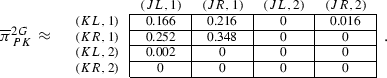
Essentially, since the entry at ((KL, 1), (JR, 2)) is positive, this indicates that the goalkeepers jumped right a little more than optimal, and since the entry ((KL, 2), (JR, 1)) is (barely) positive, this indicates that the kickers kicked left very slightly more than optimal. The remaining entries with (KL, 1), (KR, 1), (JL, 1), and (JR, 1) are all consistent with rationality.
The games and frequencies of play are taken from Goeree and Holt (2001).
We are grateful to Rahul Bhui and Peter Bossaerts for kindly providing us the data for this game.
These are taken from Costa-Gomes et al. (2001). We are grateful to Miguel Costa–Gomes for kindly providing us the data for these experiments.
Kneeland (2015) estimates for an interesting class of “ring games” the degrees to which agents are rational, hold beliefs of opponents being rational, and consistency of beliefs, and deduces that deviations from “equilibrium behavior” are largely due to inconsistency of beliefs.
To see this, notice that the computation of the largest \(\overline{p}\) consistent with payoff maximization and no further constraint must yield a no smaller \(\overline{p}\) than the same computation with the additional constraint of the common prior assumption.
To see that in a (1, 0)-rational belief system the total mass of states where agents are nonrational is unrestricted, take the game in Example 1 and consider the belief system B, where \(\Omega =A\), \(\alpha _{i}(a_{-i};a_{i})=a_{i}\), for any player i and any \(\left( a_{-i};a_{i}\right) \in A\), and where \(\mu \in \Delta (A)\) is given by \(\mu _{TL}=\mu _{TR}=\mu _{BL}=0\) and \(\mu _{BR}=1\). It can be checked that it is (1, 0)-rational and clearly \(\mu [R]=0\). At the same time, in a (p, q)-rational belief system it is always the case that, for any player i and any state \(\omega \), \(\mu (\omega )\left[ R_{-i}\right] \ge q\), hence
$$\begin{aligned} \mu [R_{-i} \cap \Pi _{i}\left( \omega \right) ] \ge q\cdot \mu [\Pi _{i}\left( \omega \right) ]\Longrightarrow \sum _{\Pi _{i}\left( \omega \right) \in \Pi _{i}} \mu [R_{-i} \cap \Pi _{i}\left( \omega \right) ]=q\cdot \sum _{\Pi _{i}\left( \omega \right) \in \Pi _{i}} \mu [\Pi _{i}\left( \omega \right) ]\Longrightarrow \mu [R_{-i}] \ge q \end{aligned}$$which besides confirming the expected convergence to the correlated equilibria as \((p,q) \rightarrow (1,1)\), also shows that positive q’s do put restrictions on the total mass of states where agents are rational \(\mu [R]\).
In order to see it in detail, given game G and probability p we say that a family of distributions \(\left( \pi _{i}\right) _{i\in I}\in \left( \Delta \left( A\right) \right) ^{I}\) is a p-subjectively rational outcome of G (p-SRO(G)) if there exists some belief system B that satisfies MB\(^{p}\)R, does not satisfy the common prior assumption and induces subjective outcomes \((\pi _{i})_{i\in I}\). As shown in the Appendix, it is easy to see that, for any \(p \in [0,1]\), the whole space is obtained, namely:
$$\begin{aligned} p- SRO\left( G\right) =\left( \Delta \left( A\right) \right) ^{I}. \end{aligned}$$In particular, a player who is certain that all the other agents are rational may still select a nonrational action, and thus, any pure strategy profile in A is consistent with MB\(^{p}\)R, even when \(p=1\).
Recall that the result of part (i) of Lemma 1 also holds with noncommon priors.
We abbreviate, \(\mu \left[ \prod _{j\ne i}(A_{j}\times \{k\})\cap \Pi _{i}(\omega )\right] =\mu \left[ \left( T\times \prod _{j\ne i}(A_{j}\times \{k\})\times A_{i}'\times \Theta \right) \cap \Pi _{i}(\omega )\right] \), with some abuse of notation.
This follows from \(p^n \ge p^{n-1}\), and because \(\pi \in p\)-RO(G) with \(p \ge p^{n-1}\) implies \(\pi \left[ \left( A^{n-1}\right) ^c \right] \le 1-p\).

References
Aliprantis CD, Border KC (2006) Infinite dimensional analysis: a Hitchhiker’s guide, 3rd edn. Springer, Berlin
Aumann RJ (1974) Subjectivity and correlation in randomized strategies. J Math Econ 1:67–96
Aumann RJ (1987) Correlated equilibria as an expression of Bayesian rationality. Econometrica 55(1):1–18
Aumann RJ (1992) Irrationality in game theory. In: Dasgupta P, Gale D, Hart O, Maskin E (eds) Economic analysis of markets and games: essays in honor of Frank Hahn. MIT Press, Cambridge
Aumann RJ, Dreze JH (2008) Rational expectations in games. Am Econ Rev 98:72–86
Battigalli P, Di Tillio A, Grillo E, Penta A (2011) Interactive epistemology and solution concepts for games with asymmetric information. BE J Theor Econ 11, Article 6
Bergemann D, Morris S (2015) Bayes correlated equilibrium and the comparison of information structures in games. forthcoming Theoretical Economics
Bernheim BD (1984) Rationalizable strategic behaviour. Econometrica 52:1007–1028
Börgers T (1994) Weak dominance and approximate common knowledge. J Econ Theor 64:265–276
Brandenburger A, Dekel E (1987) Rationalizability and correlated equilibria. Econometrica 55:1391–1402
Camerer CF (2003) Behavioral game theory: experiments in strategic interaction. Princeton University Press, New York
Camerer CF, Ho T-H (2015) Behavioral game theory, experiments and modeling. In: Young HP, Zamir S (eds) Handbook of game theory, vol 4. North-Holland, Elsevier, Amsterdam
Camerer CF, Loewenstein G, Rabin M (2011) Advances in behavioral economics. Princeton University Press, Princeton
Chiappori PA, Levitt SD, Groseclose T (2002) Testing mixed-strategy equilibria when players are heterogeneous: the case of penalty kicks in soccer. Am Econ Rev 92:1138–1151
Conlisk J (1996) Why bounded rationality? J Econ lit 34:669–700
Costa-Gomes M, Crawford VP, Broseta B (2001) Cognition and behavior in normal-form games: an experimental study. Econometrica 69:1193–1235
Crawford VP (2013) Boundedly rational versus optimization-based models of strategic thinking and learning in games. J Econ Lit 51:512–527
Dekel E, Fudenberg D, Morris S (2007) Interim correlated rationalizability. Theor Econ 2:15–40
Forges F (1993) Five legitimate definitions of correlated equilibrium in games with incomplete information. Theor Decis 35:277–310
Forges F (2006) Correlated equilibrium in games with incomplete information revisited. Theor Decis 61:329–344
Germano F, Weinstein J, Zuazo-Garin P (2016) Uncertain rationality, depth of reasoning and robustness in games with incomplete information. Mimeo
Goeree JK, Holt CA (2001) Ten little treasures of game theory and ten intuitive contradictions. Am Econ Rev 91:1402–1422
Harstad RM, Selten R (2013) Bounded-rationality models: tasks to become intellectually competitive. J Econ Lit 51:496–511
Hart S (2005) Adaptive heuristics. Econometrica 73:1401–1430
Hart S, Mansour Y (2010) How long to equilibrium? The communication complexity of uncoupled equilibrium procedures. Games Econ Behav 69:107–126
Hu T-W (2007) On p-rationalizability and approximate common certainty of rationality. J Econ Theor 136:379–391
Kajii A, Morris S (1997) Refinements and higher order beliefs: a unified survey. Mimeo
Kajii Atsushi, Morris Stephen (1997b) The Robustness of Equilibria to Incomplete Information Games. Econometrica 65:1283–1309
Kneeland T (2015) Identifying higher-order rationality. Econometrica 83:2065–2079
Lehrer E, Rosenberg D, Shmaya E (2010) Signaling and mediation in games with common interest. Games Econ Behav 68:670–682
Lehrer E, Rosenberg D, Shmaya E (2013) Garbling of signals and outcome equivalence. Games Econ Behav 81:179–191
Mallard G (2011) Modeling cognitively bounded rationality: an evaluative taxonomy. J Econ Surveys 26:674–704
Martin Christopher F, Bhui R, Bossaerts P, Matsuzawa T, Camerer C (2014) Chimpanzee choice rates in competitive games match equilibrium game theory predictions. Sci Rep 4:5182.1–6
McKelvey RD, Palfrey TR (1995) Quantal Response equilibria for normal form games. Games Econ Behav 10:6–38
Monderer D, Samet D (1989) Approximating common knowledge with common beliefs. Games Econ Behav 1:179–190
Palacios-Huerta I (2003) Professionals play minimax. Rev Econ Stud 70:395–415
Palacios-Huerta I, Volij O (2008) Experiencia docet: professionals play minimax in laboratory experiments. Econometrica 76:71–115
Pearce DG (1984) Rationalizable strategic behaviour and the problem of perfection. Econometrica 52:1029–1050
Rubinstein A (1998) Modelling bounded rationality. MIT Press, Cambridge
Stahl DO II, Wilson PW (1994) Experimental evidence on players’ models of other players. J Econ Behav Org 25:309–327
Stahl DO II, Wilson PW (1995) On players’ models of other players: theory and experimental evidence. Games Econ Behav 10:218–254
Tan Tommy Chin-Chiu, da Costa Werlang Ribeiro Sérgio (1988) The Bayesian foundation of solution concepts of games. J Econ Theor 45:370–391
Wright JR, Leyton-Brown K (2014) Level-0 meta-models for predicting human behavior in games. In: Proceedings of the 15th Conference on Economics and Computation (EC’14)
Author information
Authors and Affiliations
Corresponding author
Additional information
Earlier versions of this paper circulated under the title “Approximate Knowledge of Rationality and Correlated Equilibria.” We are indebted to Bob Aumann, Eddie Dekel, Sergiu Hart, and Dov Samet, for valuable comments and conversations. We also thank an anonymous referee and the editor, Bernhard von Stengel, as well as audiences in Barcelona, Bilbao, Budapest, Chicago, Istanbul, Jerusalem, Marseille, Paris, and York for insightful comments. Germano acknowledges financial support from the Spanish Ministry of Economy and Competitiveness (Grant ECO2014-59225-P), as well as from the Barcelona GSE Research Network and the Generalitat de Catalunya. Zuazo-Garin acknowledges financial support from the Spanish Ministry of Science and Technology (Grant ECO2009-11213), from the Spanish Ministry of Economy and Competitiveness (Grant ECO2012-31326) and from the Basque Government (Grants IT568-13 and POS-2015-1-0022), as well as inestimable help from professors Elena Iñarra and Annick Laruelle. Both authors thank the Center for the Study of Rationality at the Hebrew University of Jerusalem for their generous hospitality; Germano also thanks AMSE-IMéRA at Université Aix-Marseille and Zuazo-Garin thanks the Game Theory Group at Tel Aviv University and the CMS-EMS at Northwestern University for their generous hospitality. All errors are our own.
Appendices
APPENDIX
1.1 A Proof of Lemma 1
-
(i)
The left implication is obvious, so let’s focus on the right one. By definition, \(CB^{p}\left( R\right) \subseteq \bigcap _{i\in I}B_{i}^{p}\left( R\right) \), and therefore, for any \(i\in I\), \(CB^{p}\left( R\right) \subseteq B_{i}^{p}\left( R_{i}\right) \). Then, since \(p>0\), and \(\omega \in B_{i}^{p}\left( R_{i}\right) \), we have that \(R_{i}\cap \Pi _{i}\left( \omega \right) \ne \emptyset \), and therefore, that \(\Pi _{i}\left( \omega \right) \subseteq R_{i}\) and, in particular, \(\omega \in R_{i}\). Thus, \(B_{i}^{p}\left( R_{i}\right) \subseteq R_{i}\).
-
(ii)
It is immediate that \(CB^{1}\left( R\right) =\Omega \) if and only of \(\bigcap _{i\in I}B_{i}^{1}\left( R\right) =\Omega \), so it suffices to prove that \(\bigcap _{i\in I}B_{i}^{1}\left( R\right) =\Omega \) if and only if \(\bigcap _{i\in I}B_{i}^{1}\left( R_{-i}\right) =\Omega \). The right implication is immediate. For the proof of the left one, from part (i) of the lemma, it is enough to check that if \(\bigcap _{i\in I}B_{i}^{1}\left( R_{-i}\right) =\Omega \) then \(R=\Omega \). But this is immediate: take \(i,j\in I\), \(i\ne j\), then \(B_{j}^{p_{j}}\left( R_{-j}\right) \subseteq B_{j}^{p_{j}}\left( R_{i}\right) \), and therefore, \(B_{j}^{p_{j}}\left( R_{i}\right) =\Omega \). Hence \(\mu \left( R_{i}\right) = \sum _{\omega \in \Omega } \mu \left( R_{i}\cap \Pi _{j}\left( \omega \right) \right) = \sum _{\omega \in \Omega } \mu \left( \Pi _{j}\left( \omega \right) \right) =1\). Since \(\mu \) has full support on \(\Omega \), the latter implies that \(R_{i}=\Omega \). As the proof applies for any \(i\in I\), we obtain that \(R=\Omega \).
-
(iii)
If \(\bigcap _{i\in I}B_{i}^{p}\left( R_{-i}\right) =\Omega \), then \(R=\bigcap _{i\in I}\left( B_{i}^{p}\left( R_{-i}\right) \cap R_{i} \right) =\bigcap _{i\in I}B_{i}^{p}\left( R\right) \). Thus, R is p-evident belief and therefore, \(R\subseteq CB^{p}(R)\). Now, since \(\bigcap _{i\in I}B_{i}^{p}\left( R_{-i}\right) =\Omega \), we have both that \(\mu \left[ R_{-i}\right] \ge p\) and \(\mu \left[ R_{-i}\cap R_{i}\right] \ge p\cdot \mu \left[ R_{i}\right] \). The former implies that that \(\mu [R_{j}]\ge p\) for any \(j\ne i\); and thus, the same argument and some reindexing imply that \(\mu [R_{i}]\ge p\). The fact that for any \(j\ne i\), \(\mu \left[ R\right] =\mu \left[ R_{-i}|R_{i}\right] \cdot \mu \left[ R_{i}\right] \ge p\cdot \mu \left[ R_{i}\right] \ge p^{2}\) completes the proof.
B Proofs of the characterization results
In this section we first prove a technical lemma. Then we prove Theorem 4, and then Theorem 1 as a special case of Theorem 4. The technical lemma is the following:
Lemma 2
Let \(\left( G,S\right) \) be a Bayesian game, p a probability, \(n\in \{2,3\}\), and \(\pi ^{*}\in \left( A_{(k)}, p\right) \)-\(BCE\left( nG,S\right) \) for some \(k\le n\). For game nG, let belief system \(B=\left\langle \Omega ,\left( \Pi _{i}\right) _{i\in I},\mu ,\kappa ,\left( \alpha _{i}\right) _{i\in I},\left( \tau _{i}\right) _{i\in I}\right\rangle \) be given by: (i) \(\Omega =\left\{ \left( t,a,\nu ,\theta \right) \in T\times A'\times \Theta \right. \left. \left| \pi ^{*}\left[ \left( a,\nu ,\theta \right) \right] >0\right. \right\} \), and for any \(\left( t,a,\nu ,\theta \right) \in \Omega \), (ii) \(\mu \left[ (t,a,\nu ,\theta )\right] =\pi ^{*}\left[ \left( t,a,\nu ,\theta \right) \right] \), (iii) \(\kappa \left( t,a,\nu ,\theta \right) =\theta \), and for any \(i\in I\), (iv) we have cells \(\Pi _{i}\left( t,a,\nu ,\theta \right) =T_{-i}\times A'_{-i}\times \Theta \times \left\{ (t_{i},a_{i},\nu _{i})\right\} \), (v) \(\alpha _{i}\left( t,a,\nu ,\theta \right) =a_{i}\), and (vi) \(\tau _{i}\left( t,a,\nu ,\theta \right) =t_{i}\). Then, B is a belief system for (G, S) satisfying consistency, MB\(^{p}\)R and the common prior assumption, and induces \(\pi ^{*}\) in \(T\times A'\times \Theta \).
Proof
It is immediate that \(\alpha _{i}\) and \(\tau _{i}\) are measurable w.r.t. \(\Pi _{i}\) for any \(i\in I\). Take \(\left( t,\theta \right) \in T\times \Theta \); then, we have \(\mu \left[ \tau =t,\kappa =\theta \right] =\pi ^{*}\left[ \left( t,\theta \right) \right] =\psi \left[ \theta \right] \cdot \sigma \left[ t|\theta \right] \), and therefore, B satisfies consistency. Now, note first the fact that for any \(\omega =(t,a,\nu ,\theta )\in \Omega \) and any \(a'_{i}\in A_{i}\) it holds that,
together with the incentive constraints, implies that for any \(i\in I\) we have that \(T\times A_{-i}'\times (A_{i}\times \{k\})\times \Theta \subseteq R_{i}\), and therefore,Footnote 24 that \(\mu \left[ \prod _{j\ne i}(A_{j}\times \{k\})\cap \Pi _{i}(\omega )\right] \le \mu \left[ R_{-i}\cap \Pi _{i}(\omega )\right] \) for any \(i\in I\) and any \(\omega \in \Omega \). Then, take \(i\in I\) and \(\omega =(t,a,\nu ,\theta )\in \Omega \) and note that:
In consequence, due to the p-belief constraints, we have \(\mu \left[ R_{-i}\cap \Pi _{i}(\omega )\right] \ge p\cdot \mu \left[ \Pi _{i}(\omega )\right] \), and therefore, that B satisfies MB\(^{p}\)R. \(\square \)
1.1 B.1 Proof of Theorem 4
For the right inclusion, pick \(\pi \in p\)-\(RBO\left( G,S\right) \) and B, a belief model that induces \(\pi \). Take distribution \(\pi ^{*}\in \Delta \left( T\times A'\times \Theta \right) \) given by,
for any \((t,a,\nu ,\theta )\in T\times A'\times \Theta \). Then, \(\pi ^{*}\in \Delta \left( T\times A'\times \Theta \right) \). The consistency constraint is satisfied, since,
for any \(\left( t,\theta \right) \in T\times \Theta \). Now, note that for any \(i\in I\), any \(a_{i},a'_{i}\in A_{i}\), any \(t_{i}\in T_{i}\) and any \(\nu _{i}\in N\) we have that,
In addition, note that for any \((t_{i},a_{i},\nu _{i})\in T_{i}\times A'_{i}\),
Thus, both the incentive constraints and the p-belief constraints are satisfied. For the left inclusion, just apply Lemma 2 to \(A_{i}'=A_{i}\times \{1,2\}\) and \(k=1\).
1.2 B.2 Proof of Theorem 1
This theorem can be seen as a corollary of Theorem 4. To see this, note that if G is a game with complete information, we can define Bayesian game \(\left( G',S\right) \), where we have (i) \(G'=\left\langle I,\Theta ,\psi ,\left( A_{i}\right) _{i\in I},\left( u'_{i}\right) _{i\in I}\right\rangle \), with \(\Theta =\left\{ \theta \right\} \), \(\psi =1_{\left\{ \theta \right\} }\) and \(u'_{i}(a,\theta )=u_{i}(a)\) for any \(a\in A\) and \(i\in I\), and (ii) \(S=\left\langle \left( T_{i}\right) _{i\in I},\sigma \right\rangle \) with \(T_{i}=\left\{ t_{i}\right\} \) for any \(i\in I\) and \(\sigma (t|\theta )=1\). It is immediate that, for any \(X=\prod _{i\in I}X_{i}\subseteq A\) and any \(p\in [0,1]\), we have that \(\left( X,p\right) - CE\left( G\right) =\left( X,p\right) - BCE\left( G',S\right) \). But note also that if we take some list \(B'=\left\langle \Omega ,\left( \Pi _{i}\right) _{i\in I},\left( \alpha _{i}\right) _{i\in I},\left( \tau _{i}\right) _{i\in I},\mu \right\rangle \), which is a candidate to be a belief system for \(G'\), for any \(i\in I\), forcefully \(\tau _{i}=1_{\left\{ t_{i}\right\} }\); and therefore, \(B'\) is a belief system for \(G'\) if and only if \(B=\left\langle \Omega ,\left( \Pi _{i}\right) _{i\in I},\left( \alpha _{i}\right) _{i\in I},\mu \right\rangle \) is a belief system for G. Thus, it is immediate that, for any \(p\in [0,1]\), we have \(p- RO\left( G\right) = p- RBO\left( G',S\right) \). So, let G be a game, and \(p\in [0,1]\). Then, we just checked above that both \(p- RO\left( G\right) =p- RBO\left( G',S\right) \) and \(\left( A_{(1)},p\right) - CE\left( 2G\right) =\left( A_{(1)},p\right) - BCE\left( 2G',S\right) \), hold, so from Theorem 4 we conclude that \(p- RO\left( G\right) = \left( A_{(1)},p\right) - CE\left( 2G\right) \).
1.3 B.3 Proof of Theorem 3
We prove the first statement; the next one concerning the p-rational expectations of rational types then follows directly. We suppose we are taking some player i’s expectation. For right inclusion, take p-rational belief system \(B=\left\langle \Omega ,\left( \Pi _{i}\right) _{i\in I},\left( \alpha _{i}\right) _{i\in I},\mu \right\rangle \) and \(\omega \in \Omega \). We define:
for any \((a,\nu )\in A'\), where \(W_{i}=R_{i}{\setminus }\Pi _{i}\left( \omega \right) \) if \(\nu _{i}=0\), \(W_{i}=\lnot \left( R_{i}{\setminus }\Pi _{i}\left( \omega \right) \right) \) if \(\nu _{i}=1\), and \(W_{i}=\Pi _{i}\left( \omega \right) \) if \(\nu _{i}=2\). It is immediate that \(\pi _{i,\omega }^{*}\in \Delta \left( A'\right) \). By an argument similar to the one in the first part of the proof of Theorem 4, reduced to the degenerate case where \(|\Theta |=1\), we can conclude that \(\pi _{i,\omega }\) is a \(\left( A_{(1)},p\right) \)-correlated equilibrium of G; moreover, it is immediate that player i’s expectation conditional on playing \(\left( \alpha _{i}\left( \omega \right) ,3\right) \) induced by \(\pi _{i,\omega }\) is exactly \(\mathbb {E}(\omega )\left[ u_{i}\left( \alpha _{-i},\alpha _{i}\left( \omega \right) \right) \right] \). For the left inclusion, take Lemma 2 for the case \(A'_{i}=A_{i}\times \{1,2,3\}\), \(k=1\), and \(|\Theta |=1\).
C Proof of Theorem 2
Nonemptiness follows from the fact that correlated equilibria always exist for any finite game G and constitute p-rational outcomes for any \(p\in [0,1]\). Given that the set of p-rational outcomes is a projection of the (X, p)-correlated equilibria of 2G, with \(X=A_{(k)}\) a copy of the action space of the original game G, the remaining properties follow once they have been shown for the (X, p)-correlated equilibria of 2G. This is what we do next. For the given game G, define the (X, p)-correlated equilibrium correspondence, where \(X=A _{(k)}\) with \(k \in \{0, 1\}\), is fixed:

Clearly \(\rho \) is convex- and compact-valued; it remains to be shown that it is also continuous. We do this by showing that it is upper- and lower-hemicontinuous (respectively, uhc and lhc) as a correspondence of p.

Since 2A is finite, \(\Delta (2A)\) is compact, and hence upper-hemicontinuity is equivalent to showing that \(\rho \) has a closed graph. But this is immediate from inspection of the inequalities defining the sets \((X, p)- CE\left( 2G\right) \). In particular, all the inequalities are all weak inequalities, linear in p. Moreover, the domain [0, 1] is compact.

Denote by \(\Gamma _{\rho } \subset [0,1]\times \Delta (2A)\) the graph of the correspondence \(\rho \). Fix \((p, \hat{\pi }) \in \Gamma _{\rho }\) and let \(\left( p^n\right) _n \subset [0,1]\) be a sequence converging to p. We need to show that there exists a sequence \(\left( (\hat{\pi })^n\right) _n\) converging to \(\hat{\pi }\) such that \((\hat{\pi })^n \in \rho (p^n)\) for sufficiently large n. Take the point \((p, \hat{\pi })\). Clearly this satisfies all inequalities defining \(\rho (p)\), in particular also the p-rationality constraints. Consider the following sequence \(\left( p^n, \hat{\pi }\right) _n \subset [0,1] \times \Delta (2A)\). If for sufficiently large n the elements are contained in \(\Gamma _{\rho }\) we are done. So consider the case where they are not. Consider the family of projections \(\Pi _{\rho }: [0,1] \times \Delta (2A) \longrightarrow [0,1] \times \Delta (2A)\) that map, for fixed \(\bar{p} \in [0,1]\), any element \((\bar{p}, \bar{\pi }) \in [0,1] \times \Delta (2A)\) to the point in the set \(\{ \bar{p} \} \times \rho ( \bar{p} )\) that is closest to \((\bar{p}, \bar{\pi })\). Since the sets \(\rho ( \cdot )\) are always nonempty, convex, compact polyhedra, we have that \(\Pi _{\rho } \left( p^n, \hat{\pi } \right) \) is uniquely defined and moreover, \(\Pi _{\rho } \left( p^n, \hat{\pi } \right) \in \Gamma _{\rho }\) for any point in the sequence \(\left( p^n, \hat{\pi } \right) _n\). It remains to be shown that the sequence \(\left( \Pi _{\rho } \left( p^n, \hat{\pi } \right) \right) _n\) converges to the point \((p, \hat{\pi })\). Apart from the p-belief constraints all other constraints defining \(\rho (p)\) are independent of p. Hence, if \((p, \hat{\pi })\) satisfies those constraints, then so must any other point in the sequence \(\left( p^n, \hat{\pi }\right) _n\). Therefore the only constraints that can be violated by elements of the sequence \(\left( p^n, \hat{\pi }\right) _n\) are the p-belief constraints. Consequently, any point in the sequence \(\left( \Pi _{\rho } \left( p^n, \hat{\pi } \right) \right) _n\) lies on the boundary of the polyhedra defined by the p-belief constraints. As mentioned, these constraints are linear in p, and since they also define nonempty, convex, compact polyhedra, the sequence \(\left( \Pi _{\rho } \left( p^n, \hat{\pi } \right) \right) _n\) indeed converges to \((p, \hat{\pi })\). This shows the continuity of \(\rho \) and hence also of p-RO(G) in p.
Finally, the claims that, for \(p=0\), we have 0-\(RO(G)=\Delta (A)\), and for \(p=1\), we have 1-\(RO(G)=CE(G)\), are immediate. To see that for any \(p \in [0,1)\), we have dim[p-\(RO(G)]=\) dim\([\Delta (A)]\), notice that the (X, p)-correlated equilibria with \(X=A^1\) and \(p<1\) entail distributions that put strictly positive weight on all strategies in \(A^2\) as well as all convex combinations of such distributions. Projecting onto the original space \(\Delta (A)\) implies distributions with strictly positive weights on all strategies in A as well as all possible convex combinations. This concludes the proof.
D Proof of Proposition 1
Fix G and let \(A^n=\Pi _{i \in I} A_i^n\) denote the space of all pure strategy profiles that survive n rounds of iterated elimination of strictly dominated strategies in G, and similarly for the individual sets \(A_i^n\). Let \(G^n\) denote the subgame of G with strategies restricted to \(A^n\). Because G is finite, the limit sets \(A_i^{\infty }, A^{\infty }\), and \(G^{\infty }\) are well defined (and are obtained after finitely many iterations). Also, for any subset \(Y \subset A\), let \(Y^c=A{\setminus } Y\) denote the complement of Y in A. For any given \(p\in \left[ 0,1\right] \), take \(p'\ge p\). We show that for p sufficiently close to 1, behavior is supported with high probability in \(A^{\infty }\). Specifically, we construct a \(\bar{p}<1\) such that for any \(p \in [\bar{p}, 1]\), if \(\pi \in p\)-RO(G), then \(\pi \left[ \left( A^{\infty }\right) ^c \right] \le 1-p\). Consider the game \(G^0=G\) and pick some \(p^1<1\). It immediately follows from p-rationality that for \(p\in [p^1,1]\), if \(\pi \in p\)-RO(G), then we have \(\pi \left[ \left( A^1\right) ^c \right] \le 1-p\). Suppose now that the above statement is true for \(n-1\), namely there exists \(p^{n-1}<1\) such that for \(p \in [p^{n-1},1]\), if \(\pi \in p\)-RO(G), then we have \(\pi \left[ \left( A^{n-1}\right) ^c \right] \le 1-p\). We show that the statement also holds for n. Fix game \(G^{n-1}\). It follows from finiteness of G and continuity of the payoffs that there exists \(p^n \in [p^{n-1}, 1)\) such a strategy in \(A^{n-1}{\setminus } A^n\) that is strictly dominated in \(G^{n-1}\) (by some strategy in \(G^{n-1}\) and hence in G) is also strictly dominated in G (by the same strategy) given a p-rational belief system with \(p \ge p^n\).Footnote 25 This implies that for any \(p \in [p^n, 1]\) and any \(\pi \in p\)-RO(G), we also have \(\pi \left[ \left( A^n\right) ^c\right] \le 1-p\). Finiteness of the game implies that the process ends after finitely many steps implying that indeed there exists \(p^{\infty } <1\) such that for \(p \in [p^{\infty }, 1]\) and any \(\pi \in p\)-RO(G), we have \(\pi \left[ \left( A^{\infty }\right) ^c \right] \le 1-p\). Taking \(\bar{p}=p^{\infty }\) proves the claim.
E Proof of Proposition 2
To see the if part, take \(\pi \in \Delta (A)\) a p-rational outcome of G. By Theorem 1, there exists an \((A_{(1)}, p)\)-correlated equilibrium \(\hat{\pi } \in \Delta (A')\) of the doubled game 2G. Define \(P \equiv \hat{\pi }\) and set
for all \(t_{i} \in T_{i}\). Then, by definition of the type spaces \(T_{i}=T_{i}^{s} \cup T_{i}^{c}\), we have:
-
\(P[ T^{s}_{-i} \, | \, t_{i}] \ge p\), for any \(t_{i} \in T_{i}\);
-
\(\alpha _{i} (t_{i})[a_{i}]= 1\) if \(t_{i} \in T^{c}_{i}\) and \(t_{i}= a_{i}\)
-
\(a_{i} \in \) argmax\(_{a_{i}' \in A_{i}} \sum _{t_{-i} \in T_{-i}}P[t_{-i} \, | \, t_{i}]\cdot \sum _{a_{-i} \in A_{-i}}\alpha _{-i} (t_{-i})[a_{-i}]\cdot u_{i}(a_{-i};a_{i}')\), where \(\alpha _{-i}(t_{-i})[a_{-i}]=\prod _{j\ne i}\alpha _{j}(t_{j})[a_{j}]\).
Let \(\mu [a]=\sum _{t \in T}P(t)\cdot \alpha (t)[a]\), where \(\alpha (t)[a]=\prod _{i\in I}\alpha _{i}(t_{i})[a_{i}]\); then, again by construction, and using Theorem 1, we have \(\mu = \pi \).
To see the only if part, take \(\mu \in \Delta (A)\) an EAD of (G, P) where P satisfies \(P[ T^{s}_{-i} \, | \, t_{i}] \ge p\), for any \(t_{i} \in T_{i}\), and for some equilibrium profile \(\alpha \) satisfying conditions (i) and (ii). By definition, together with P, \(\alpha \) can be seen as inducing a probability distribution on the outcomes of the doubled game \(\hat{\mu } \in \Delta (2A)\), where types in \(T_{i}^{s}\) and corresponding strategies chosen are associated to \(A_{(2)}\) and types in \(T_{i}^{c}\) are associated to strategies in \(A_{(2)}\). As a consequence of (i) and (ii) and the definition of P, \(\hat{\mu }\) will also satisfy the incentive constraints and the p-belief constraints for 2G. By Theorem 1, computing the EAD \(\mu \) of \(\hat{\mu }\) gives us, a p-rational outcome of G.
F Proof of result in Remark 2
Adapting the original definition by Aumann (1974), Aumann (1987), for any \(X=\prod _{i\in I}X_{i}\subseteq A\), we say that the family \(\left( \pi _{i}\right) _{i\in I}\subseteq \left( \Delta \left( A\right) \right) ^{I}\) is a \(\left( X,p\right) \)-subjective correlated equilibrium of G, if, for any \(i\in I\) the following are satisfied:
-
Incentive constraints For any \(a_{i}\in X_{i}\), \(a_{i}\in \text {argmax}_{a'_{i}\in A_{i}}\sum _{a_{-i}\in A_{-i}}\pi _{i}[\left( a_{-i};a_{i}\right) ]\cdot u_{i}\left( a_{-i};a'_{i}\right) \).
-
p-Belief constraints For any \(a_{i}\in A_{i}\), \(\pi _{i}\left[ X_{-i}\times \{a_{i}\}\right] \ge p\cdot \pi _{i}\left[ A_{-i}\times \{a_{i}\}\right] \).
We denote the set of \(\left( X,p\right) \)-subjective correlated equilibria of game G by \(\left( X,p\right) - SCE\left( G\right) \). Given \(n\in \{2,3\}\) and nG, we have a map \(\mathbf marg _{A^{I}}:\left( \Delta \left( A'\right) \right) ^{I}\rightarrow \left( \Delta \left( A\right) \right) ^{I}\), where for any \(\left( \hat{\pi _{i}}\right) _{i\in I}\in \left( \Delta \left( A'\right) \right) ^{I}\), we have that \(\mathbf{marg }_{A^{I}}\left( \left( \hat{\pi _{i}}\right) _{i\in I}\right) =\left( \text {marg}_{A}\left( \hat{\pi _{i}}\right) \right) _{i\in I}\). Then, the proof of the identity,
where \(X=\prod _{i\in I}\left( A_{i}\times \left\{ 1\right\} \right) \), is the same as the one for Theorem 1 after slight modifications (just add sub-indices where needed). To see that the above marginals constitute the whole space, take \(\left( a^{i}\right) _{i\in I}\subseteq A\), and for any \(i\in I\), \(\pi _{i}=1_{\left\{ a^{i}\right\} }\). Fix \(k\in \left\{ 1,2\right\} \), and define, for any \(i\in I\), \(\hat{\pi }_{i}=1_{\{((a_{j}^{i},k)_{j\ne i};(a_{i}^{i},2-k))\}}\). It is immediate that \(\mathbf{marg }_{A^{I}}\left( \left( \hat{\pi }_{i}\right) _{i\in I}\right) =\left( \pi _{i}\right) _{i\in I}\). Now, take \(i\in I\), then the incentive constraints are trivially satisfied, since \(\hat{\pi }_{i}[A_{i}\times \left\{ 1\right\} ]=0\). Moreover, the p-belief constraint is also satisfied, because, regardless of i’s action, the sums are on both sides 0 or 1. We conclude that, again for \(X=\prod _{i\in I}\left( A_{i}\times \left\{ 1\right\} \right) \), we have \(\left( 1_{\{a^{i}\}}\right) _{i\in I}\in \mathbf{marg }_{A^{I}}((X ,p)- SCE(2G))\) for any \((a^{i})_{i\in I}\subseteq A\); thus, by convexity, \(\mathbf{marg }_{A^{I}}((X ,p)- SCE(2G))=((\Delta \left( A\right) )^{I}\).
Rights and permissions
About this article

Cite this article
Germano, F., Zuazo-Garin, P. Bounded rationality and correlated equilibria. Int J Game Theory 46, 595–629 (2017). https://doi.org/10.1007/s00182-016-0547-5
Accepted:
Published:
Issue Date:
DOI: https://doi.org/10.1007/s00182-016-0547-5
Keywords
- Strategic interaction
- Correlated equilibrium
- Robustness to bounded rationality
- Approximate knowledge
- Incomplete information
- Measure of rationality
- Experiments