
Abstract
This paper introduces the shape mixtures of the skew-t-normal distribution which is a flexible extension of the skew-t-normal distribution as it contains one additional shape parameter to regulate skewness and kurtosis. We study some of its main characterizations, showing in particular that it is generated through a mixture on the shape parameter of the skew-t-normal distribution when the mixing distribution is normal. We develop an Expectation Conditional Maximization Either algorithm for carrying out maximum likelihood estimation. The asymptotic standard errors of estimators are obtained via the information-based approximation. The numerical performance of the proposed methodology is illustrated through simulated and real data examples.


References
Adcock C, Eling M, Loperfido N (2015) Skewed distributions in finance and actuarial science: a review. Eur J Financ 21:1253–1281
Aitken AC (1927) On Bernoulli’s numerical solution of algebraic equations. Proc R Soc Edinb 46:289–305
Akaike H (1973) Information theory and an extension of the maximum likelihood principle. In: Petrov BN, Csaki F (eds) 2nd International symposium on information theory. Akademiai Kiado, Budapest, pp 267–281
Anscombe FJ, Glynn WJ (1983) Distribution of the kurtosis statistic \(b_2\) for normal statistics. Biometrika 70:227–234
Arellano-Valle RB, Castro LM, Genton MG, Gómez HW (2008) Bayesian inference for shape mixtures of skewed distributions, with application to regression analysis. Bayesian Ana 3:513–540
Arellano-Valle RB, G ómez HW, Quintana FA (2004) A new class of skew-normal distributions. Commun Stat Theory Methods 33:1465–1480
Azzalini A (1985) A class of distributions which includes the normal ones. Scand J Stat 12:171–178
Azzalini A with the collaboration of Capitanio A (2014) The skew-normal and related families, IMS monographs. Cambridge University Press, Cambridge
Azzalini A, Capitaino A (2003) Distributions generated by perturbation of symmetry with emphasis on a multivariate skew \(t\)-distribution. J R Stat Soc B 65:367–389
Branco MD, Dey DK (2001) A general class of multivariate skew-elliptical distributions. J Multivar Anal 79:99–113
Cramér H (1946) Mathematical methods of statistics. Princeton University Press, Princeton
Dempster AP, Laird NM, Rubin DB (1977) Maximum likelihood from incomplete data via the EM algorithm (with discussion). J R Stat Soc B 39:1–38
D’Agostino RB (1970) Transformation to normality of the null distribution of g1. Biometrika 57:679–681
Efron B, Hinkley DV (1978) Assessing the accuracy of the maximum likelihood estimator: observed versus expected Fisher information. Biometrika 65:457–482
Efron B, Tibshirani R (1986) Bootstrap methods for standard errors, confidence intervals, and other measures of statistical accuracy. Stat Sci 1:54–75
Eling M (2012) Fitting insurance claims to skewed distributions: are the skew-normal and skew-student good models? Insur Math Econ 51:239–248
Eling M (2014) Fitting asset returns to skewed distributions: are the skew-normal and skew-student good models? Insur Math Econ 59:45–56
Ferreira CS, Bolfarine H, Lachos VH (2011) Skew scale mixture of normal distributions: properties and estimation. Stat Method 8:154–171
Gómez HW, Venegas O, Bolfarine H (2007) Skew-symmetric distributions generated by the distribution function of the normal distribution. Environmetrics 18:395–407
Ho HJ, Lin TI, Chang HH, Haase HB, Huang S, Pyne S (2012a) Parametric modeling of cellular state transitions as measured with flow cytometry different tissues. BMC Bioinform 13:S5
Ho HJ, Pyne S, Lin TI (2012b) Maximum likelihood inference for mixtures of skew student-\(t\)-normal distributions through practical EM-type algorithms. Stat Comput 22:287–299
Huber PJ (1967) The behavior of maximum likelihood estimates under nonstandard conditions. In: Proceedings of the fifth Berkeley symposium on mathematical statistics and probability, vol 1. University of California Press, Berkeley, pp 221–233
Jamalizadeh A, Lin TI (2017) A general class of scale-shape mixtures of skew-normal distributions: properties and estimation. Comput Stat 32:451–474
Lin TI, Lee JC, Yen SY (2007) Finite mixture modelling using the skew normal distribution. Stat Sin 17:909–927
Lin TI, Ho HJ, Lee CR (2014) Flexible mixture modelling using the multivariate skew-t-normal distribution. Stat Comput 24:531–546
Liu CH, Rubin DB (1994) The ECME algorithm: a simple extension of EM and ECM with faster monotone convergence. Biometrika 81:633–648
Meng XL, Rubin DB (1993) Maximum likelihood estimation via the ECM algorithm: a general framework. Biometrika 80:267–278
Meng XL, van Dyk D (1997) The EM algorithm-an old folk-song sung to a fast new tune (with discussion). J R Stat Soc B 59:511–567
Schwarz G (1978) Estimating the dimension of a model. Ann Stat 6:461–464
Smirnov NV (1948) Tables for estimating the goodness of fit of empirical distributions. Ann Math Stat 19:279–281
Wang WL, Lin TI (2013) An efficient ECM algorithm for maximum likelihood estimation in mixtures of \(t\)-factor analyzers. Comput Stat 28:751–769
Wu CFJ (1983) On the convergence properties of the EM algorithm. Ann Stat 11:95–103
Wu LC (2014) Variable selection in joint location and scale models of the skew-\(t\)-normal distribution. Commun Stat Simul Comput 43:615–630
Acknowledgements
We gratefully acknowledge the chief editor, the associate editor and two anonymous referees for their valuable comments and suggestions, which led to a greatly improved version of this article. This research was supported by MOST 105-2118-M-005-003-MY2 awarded by the Ministry of Science and Technology of Taiwan.
Author information
Authors and Affiliations
Corresponding author
Electronic supplementary material
Below is the link to the electronic supplementary material.
Appendices
Appendix A: The score function and Hessian matrix
From (14), the log-likelihood function corresponding to the jth observation is
where \(u_{j}=(y_{j}-\xi )/\sigma \). Let \(s_{j}(\varvec{\theta })=(s_{j,\xi },s_{j,\sigma },s_{j,\lambda },s_{j,\alpha },s_{j,\nu })\) be a \(5\times 1\) vector. Based on the definition of \(s_{j}(\varvec{\theta })\) in Sect. 3.2, explicit expressions for the components of \(s_{j}(\varvec{\theta })\) are obtained by differentiation from (A.1) with respect to each parameter. They are given by
where \(\zeta _{j}=(\nu +1)/(\nu +u_{j}^{2})\), \(\omega _{j}=(1+\alpha u_{j}^{2})^{3/2}\) and \(R_{j}=\phi (\lambda u_{j}\omega _{j}^{-1/3})/\varPhi (\lambda u_{j}\omega _{j}^{-1/3})\). The Hessian matrix consisting of the second partial derivatives of the SMSTN log-likelihood takes the form of
The detailed expressions for the components of \(H_{j}(\varvec{\theta })\) are shown below.
where \(H_j^{\theta _r\theta _s}=H_j^{\theta _s\theta _r}\), \(A_j=\lambda R_{j}+\lambda ^{2}u_{j}\omega _{j}^{-1/3}\) and \(\mathrm{TG}(x)=d^{2}\log \varGamma (x)/dx^{2}\) is the trigamma function.
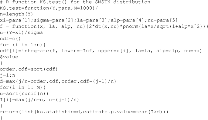
Appendix B: The procedure of the Kolmogorov–Smirnov test for continuous data
-
1.
Sort data values into ascending order \(y_{(1)}\le y_{(2)}\le \cdots \le y_{(n)}\).
-
2.
Compute the KS test statistic
$$\begin{aligned} D=\mathop {\max _{j=1,\ldots ,n}}\left\{ \frac{j}{n}-\hat{F}(y_{(j)}),~\hat{F}(y_{(j)})-\frac{j-1}{n}\right\} , \end{aligned}$$where \(\hat{F}(\cdot )\) is the fitted cdf under a specific distribution.
-
3.
Generate n random number from U(0, 1) and sort them into ascending order, we have \(u^{(i)}_{(1)}\le u^{(i)}_{(2)} \le \cdots \le u^{(i)}_{(n)}\) for \(i=1,\ldots ,n\).
-
4.
Compute
$$\begin{aligned} d_i=\mathop {\max _{j=1,\ldots ,n}}\left\{ \frac{j}{n}-u_{(j)}^{(i)},~u_{(j)}^{(i)}-\frac{j-1}{n}\right\} . \end{aligned}$$ -
5.
Set \(I_i=1\) if \(d_i\ge D\) and 0 otherwise. Repeat Steps 3 and 4 M times, we get \(I_1,...,I_M\). The p-value is estimated by \(\sum ^{M}_{i=1} I_i/M\).

Rights and permissions
About this article

Cite this article
Tamandi, M., Jamalizadeh, A. & Lin, TI. Shape mixtures of skew-t-normal distributions: characterizations and estimation. Comput Stat 34, 323–347 (2019). https://doi.org/10.1007/s00180-018-0835-6
Received:
Accepted:
Published:
Issue Date:
DOI: https://doi.org/10.1007/s00180-018-0835-6