
Abstract
Recent targeted attacks have increased significantly in sophistication, undermining the fundamental assumptions on which most cryptographic primitives rely for security. For instance, attackers launching an Advanced Persistent Threat (APT) can steal full cryptographic keys, violating the very secrecy of “secret” keys that cryptographers assume in designing secure protocols. In this article, we introduce a game-theoretic framework for modeling various computer security scenarios prevalent today, including targeted attacks. We are particularly interested in situations in which an attacker periodically compromises a system or critical resource completely, learns all its secret information and is not immediately detected by the system owner or defender. We propose a two-player game between an attacker and defender called FlipIt or The Game of “Stealthy Takeover.” In FlipIt, players compete to control a shared resource. Unlike most existing games, FlipIt allows players to move at any given time, taking control of the resource. The identity of the player controlling the resource, however, is not revealed until a player actually moves. To move, a player pays a certain move cost. The objective of each player is to control the resource a large fraction of time, while minimizing his total move cost. FlipIt provides a simple and elegant framework in which we can formally reason about the interaction between attackers and defenders in practical scenarios. In this article, we restrict ourselves to games in which one of the players (the defender) plays with a renewal strategy, one in which the intervals between consecutive moves are chosen independently and uniformly at random from a fixed probability distribution. We consider attacker strategies ranging in increasing sophistication from simple periodic strategies (with moves spaced at equal time intervals) to more complex adaptive strategies, in which moves are determined based on feedback received during the game. For different classes of strategies employed by the attacker, we determine strongly dominant strategies for both players (when they exist), strategies that achieve higher benefit than all other strategies in a particular class. When strongly dominant strategies do not exist, our goal is to characterize the residual game consisting of strategies that are not strongly dominated by other strategies. We also prove equivalence or strict inclusion of certain classes of strategies under different conditions. Our analysis of different FlipIt variants teaches cryptographers, system designers, and the community at large some valuable lessons:
-
1.
Systems should be designed under the assumption of repeated total compromise, including theft of cryptographic keys. FlipIt provides guidance on how to implement a cost-effective defensive strategy.
-
2.
Aggressive play by one player can motivate the opponent to drop out of the game (essentially not to play at all). Therefore, moving fast is a good defensive strategy, but it can only be implemented if move costs are low. We believe that virtualization has a huge potential in this respect.
-
3.
Close monitoring of one’s resources is beneficial in detecting potential attacks faster, gaining insight into attacker’s strategies, and scheduling defensive moves more effectively.
Interestingly, FlipIt finds applications in other security realms besides modeling of targeted attacks. Examples include cryptographic key rotation, password changing policies, refreshing virtual machines, and cloud auditing.
1 Introduction
The cyber-security landscape has changed tremendously in recent years. Major corporations and organizations, including the United Nations, Lockheed Martin, Google and RSA, have experienced increasingly sophisticated targeted attacks (e.g., Aurora, Stuxnet). These attacks, often referred in industry circles as Advanced Persistent Threats (APTs), exhibit several distinctive characteristics compared to more traditional malware. APTs are extremely well funded and organized, have very specific objectives, and have their actions controlled by human operators. They are in general persistent for long periods of time in a system, advancing stealthily and slowly to maintain a small footprint and reduce detection risks. Typically, APTs exploit infrastructure vulnerabilities through an arsenal of zero-day exploits and human vulnerabilities through advanced social-engineering attacks.
When designing security protocols, cryptographers and computer security researchers model adversarial behavior by making simplifying assumptions. Traditional cryptography relies for security on the secrecy of cryptographic keys (or of system state). Modern cryptography considers the possibility of partial compromise of system secrets. Leakage resilient cryptography, for instance, constructs secure primitives under the assumption that a system is subject to continuous, partial compromise. But in an adversarial situation, assumptions may fail completely. For instance, attackers launching an APT can steal full cryptographic keys, crossing the line of inviolate key secrecy that cryptographers assume in designing primitives. Assumptions may also fail repeatedly, as attackers find new ways to penetrate systems.
In this paper, motivated by recent APT attacks, we take a new perspective and develop a model in which an attacker periodically compromises a system completely, in the sense of learning its entire state, including its secret keys. We are especially interested in those scenarios where theft is stealthy or covert and not immediately noticed by the victim. We model these scenarios by means of a two-player game we call FlipIt, a.k.a. The Game of “Stealthy Takeovers”.
FlipIt is a two-player game with a shared resource that both players (called herein attacker and defender) wish to control. The resource of interest could be, for instance, a secret key, a password, or an entire infrastructure, depending on the situation being modeled. Players take control of the resource by moving, and paying a certain move cost, but unlike most existing games, in FlipIt players can move at any given time. Most importantly, a player does not immediately know when the other player moves! A player only finds out about the state of the system when she moves herself. This stealthy aspect of the game is a unique feature of FlipIt, which to the best of our knowledge has not been explored in the game theory literature. The goal of each player is to maximize a metric we call benefit, defined as the fraction of time the player controls the resource minus the average move cost. A good strategy for a given player, therefore, is one that gives the player control of the resource a large fraction of the time with few moves.
Our main goal in this paper is to find best-choice (ideally dominant or strongly dominant) playing strategies for different variants of the FlipIt game that achieve maximum benefit for each player. An instance of FlipIt is determined by the information players receive before the game, the feedback players obtain while playing the game, and a space of strategies or actions for each player. We have created a hierarchical graphical representation of different classes of strategies for one player in Fig. 1. The strategies are ordered (from top to bottom) by increasing amount of feedback received by a player during the game. As we move down the hierarchy, we encompass broader classes of strategies. In the paper, we prove results about the equivalence of different classes of strategies, (strongly) dominant and dominated strategies within a particular class, and strict inclusion of a class in a broader class. We also characterize, for several instances of FlipIt, the residual game consisting of strategies that are not strongly dominated. We detail below several FlipIt instances that we define and analyze, and then describe the theoretical results proven in the paper, as well as the results based on experimental evidence. We also discuss some of our conjectures regarding the relationship among different classes in the hierarchy, leading to some challenging open problems.

Hierarchy of strategies in FlipIt.
FlipIt Instances
Broadly, as graphically shown in Fig. 1, we define two main classes of strategies for a player: non-adaptive strategies (NA) in which the player does not receive any feedback during the game; and adaptive strategies (AD) in which the player receives certain types of feedback when moving.
In the class of non-adaptive strategies, one subclass of particular interest is that of renewal strategies. For a player employing a renewal strategy, the intervals between the player’s consecutive moves are independent and identically distributed random variables generated by a renewal process. Examples of renewal strategies include: the periodic strategy in which the interval between two consecutive moves is fixed at a constant value and the exponential strategy in which the intervals between consecutive moves are exponentially distributed. The moves of a player employing a non-adaptive (but possibly randomized) strategy can be determined before the game starts, as there is no feedback received during the game.
In the class of adaptive strategies, we distinguish a subclass called last move or LM, in which the player finds out upon moving the exact time when his opponent moved last. In a general adaptive strategy, a player receives upon moving complete information about his opponent’s moves (this is called full history or FH). Classes LM and FH collapse in some cases (for instance when the opponent plays with a renewal strategy).
A further dimension to a player’s strategy is the amount of information the player receives before the game starts. Besides the case in which the player receives no information about his opponent before the game, other interesting cases are: (1) rate-of-play (or RP), in which the player finds out the exact rate of play of his opponent; (2) knowledge-of-strategy (KS), in which the player finds out full information about the strategy of the opponent (but not the opponent’s randomness).
Contributions and Results
Our first contribution in this paper is the definition of the FlipIt game, and its application to various computer security scenarios, including APTs. We view FlipIt as a theoretical framework that helps provide a foundation for the science of cyber-security.
We then analyze several instances of the game of increasing sophistication and complexity. Our main theoretical and experimental results, as well as conjectures, and remaining open questions are summarized in Table 1. To simplify the exposition, we present results for the case when the attacker is more powerful than the defender and organize these results according to the strength of the attacker. Since the game is symmetric, though, analogous results apply when the defender is more powerful than the attacker. In this article, we restrict ourselves to games in which the defender plays with a renewal strategy.
To elaborate, we start by analyzing the simple game in which both players employ a periodic strategy with a random phase. (In such a strategy, moves are spaced at equal intervals, with the exception of the first randomly selected move called the phase.) We compute the Nash equilibrium point for the periodic game and show that the benefit of the player with higher move cost is always 0 in the Nash equilibrium. When move costs of both players are equal, players control the resource evenly and both achieve benefit 0.
We next consider a variant of FlipIt in which both players play with either a renewal or periodic strategy with random phase. We call such games renewal games. Our main result for the renewal game (Theorem 4 in Sect. 4.3) shows that the periodic strategy with a random phase strongly dominates all renewal strategies of fixed rate. Therefore, we can completely characterize the residual FlipIt game when players employ either renewal or periodic strategies with random phases. It consists of all periodic strategies with random phases.
We also analyze renewal games in which the attacker receives additional information about the defender at the beginning of the game, in particular the rate of play of the defender. For this version of the game, we prove that Theorem 4 still holds, and periodic strategies are strongly dominant. Additionally, we determine in Theorem 5 in Sect. 4.4 parameter choices for the rates of play of both attacker and defender that achieve maximum benefit.
Moving towards increased sophistication in the attacker’s strategy, we next analyze several FlipIt instances for the attacker in the broad Last-Move (LM) class. The attacker in this case adaptively determines his next move based on the feedback learned during the game, in particular the exact time of the defender’s last move. In this setting, periodic play for the defender is not very effective, as the attacker learning the defender’s period and last-move time can move right after the defender and achieve control of the resource most of the time. We demonstrate in Theorem 6 in Sect. 5.3 that by playing with an exponential strategy instead, the defender forces an adaptive attacker into playing periodically. (That is, the periodic strategy is the strongly dominant attacker strategy in the class of all LM strategies against an exponential defender strategy.) Paradoxically, therefore, the attacker’s strongly dominant strategy does not make use of the full knowledge the attacker gains from the feedback received during the game. (The full hierarchy in Fig. 1 for the attacker strategy collapses for exponential defender play.) Additionally, we determine optimal parameters (i.e., parameters that optimize both players’ benefits) for both the exponential defender and periodic attacker distributions in Theorems 7 and 8 in Sect. 5.3.
For both non-adaptive and fully adaptive attacker strategies, we show that by playing periodically at sufficiently high rate, the defender can force the attacker to drop out of the game. The move cost of the defender needs to be significantly lower than that of the attacker, however, for such a strategy to bring benefit to the defender. This demonstrates that the player radically lowering his move cost relative to his opponent obtains a high advantage in the game and can effectively control the resource at all times.
We propose an enhancement to the exponential distribution employed by the defender, a strategy that we call delayed exponential. In this strategy, the defender waits after each move for some fixed interval of time and then waits for an exponentially distributed time interval until making her next move. We show experimentally that with this strategy the benefit of the defender is higher than that for exponential play. This result provides evidence that the exponential strategy is not the strongly dominant renewal defender strategy against an LM attacker. There are still interesting questions for which we cannot yet provide a definitive answer: What other renewal strategies for the defender could further increase her benefit?; Is there a strongly dominant strategy for the defender in the class of all renewal strategies against an LM attacker?
Lastly, we explore a Greedy algorithm in which the attacker’s moves are chosen to maximize the local benefit achieved in an interval between two consecutive attacker moves. We analyze the Greedy strategy for several renewal defender strategies and demonstrate that it results in the strongly dominant strategy for an exponential defender strategy. We also show one example for which the Greedy strategy does not result in a dominant strategy for the attacker. We leave open the challenging problem of which strategies are (strongly) dominant for an LM attacker against particular classes of defender strategies (e.g., renewal strategies).
Lessons Derived from FlipIt
Our analysis of FlipIt teaches cryptographers, system designers, and the community at large some valuable lessons:
-
1.
Systems should be designed under the assumption of repeated total compromise, including theft of cryptographic keys. Many times, attackers cross the line of secrey cryptographers assume in their protocol designs. This view has already been expressed by the head of the NSA’s Information Assurance Directorate [28]: “No computer network can be considered completely and utterly impenetrable—not even that of the NSA. NSA works under the assumption that various parts of their systems have already been compromised, and is adjusting its actions accordingly.”
FlipIt provides guidance on how and when to implement a cost-effective defense. For instance, our analysis can help defenders determine when they should change cryptographic keys or user credentials, and how often should they clean their machines or refresh virtual machine instances. FlipIt analysis, conversely, also guides attackers in how to schedule their attacks to have maximal effect, while minimizing attack cost.
-
2.
Aggressive play by the defender can motivate the attacker to drop out of the game (and essentially not to play at all). The best defensive strategy, therefore, is to play fast (for instance by changing passwords frequently, rebooting servers often, or refreshing virtual machines at short intervals) and make the opponent drop out of the game. To be able to move fast, the defender should arrange the game so that her moves cost much less than the attacker’s moves.
An interesting research challenge for system designers is how to design an infrastructure in which refresh/clean costs are very low. We believe that virtualization has huge potential in this respect.
-
3.
As we have shown in our theoretical analysis, any amount of feedback (even limited) received during the game about the opponent benefits a player in FlipIt. Defenders, therefore, should monitor their systems frequently to gain information about the attacker’s strategy and detect potential attacks quickly after take over. Both monitoring and fast detection help a defender more effectively schedule moves, which results in more control of the resource and less budget spent on moves, increasing the defender’s benefit.
Conjectures and Open Problems
In this paper, we introduce a new framework, reflected in the FlipIt game, for modeling different cyber-security situations. The FlipIt game is unique in the game theory literature mostly for its stealthy aspect and continuous-time play. We prove some interesting results about different variants of the game, and the relationships among several classes of strategies. Nevertheless, many interesting questions remain to be answered in order to understand fully all facets of this simple (but challenging-to-analyze) game. We elaborate here on some of the more interesting open problems we have identified, and also state some conjectures for whose truth our results provide strong evidence.
-
1.
For FlipIt with non-adaptive strategies for both defender and attacker, we have fully analyzed the subclass of renewal games. An analysis of the game in which one or both players employ general non-adaptive strategies is deferred to future work. It would be interesting to determine if periodic strategies are still dominant in the general non-adaptive FlipIt game.
-
2.
In the case in which the attacker receives additional information about the defender at the beginning of the game (e.g., the rate of play of the defender or extra information about the defender’s strategy) and both players employ non-adaptive strategies, which strategies are best choices for both players? From this class of games, we analyzed the renewal game in which one player receives RP information and the other receives no information, RP, or KS. We leave open the analysis of other instances of FlipIt in this class.
-
3.
We believe that the most interesting open questions arise in the case in which one player (e.g., the attacker) is adaptive. Here we enumerate several of them:
-
When the attacker is LM, which renewal strategies for the defender are (strongly) dominant?
-
Which LM strategies are (strongly) dominant against a renewal defender?
-
For which class of defender strategies is the Greedy algorithm (strongly) dominant for an LM attacker?
-
When the attacker is LM, the relationship between the non-adaptive and adaptive classes for the defender is not completely understood. We have though strong evidence (also deferred to follow-up work) to state the following conjecture:
-
Conjecture 1
Consider an instance of FlipIt with an LM attacker. Then the defender receiving feedback during the game and playing with an adaptive strategy can strictly improve her benefit relative to non-adaptive play.
-
4.
The most challenging instance of FlipIt is when both players utilize adaptive strategies. In this setting, it would be interesting to determine (strongly) dominant strategies (if any), and to what extent they involve cooperation among players.
2 Game Motivation
We start by defining FlipIt in an informal way. In the second part of this section, we describe several practical applications that motivated the game definition. In Sect. 3, we give a formal definition of FlipIt with careful specification of players’ action spaces, strategies, and benefits.
2.1 Game Definition by Example
Consider a resource that can be controlled (or “owned”) by either of two players (attacker or defender). Ownership will change back and forth following a move of either player, with the goal of each player being to maximize the fraction of time that he or she controls the resource. A distinctive feature of FlipIt is its stealthy aspect, that is, the players do not know when the other player has taken over. Nor do they know the current ownership of the resource unless they perform a move. Also important is the fact that to move, a player must pay a move cost; players thus have a disincentive against moving too frequently.
In an example implementation of a basic version of FlipIt, each player has a control panel with a single button and a light. The player may push his/her button at any time (in the most general form of FlipIt, we consider time to be continuous, but we support discrete variants as well). Pushing the button always causes the button-pusher to take ownership of the resource. We assume that players do not push their buttons at exactly the same time (or, if they do, then ownership does not change hands).
If pushing the button causes ownership to change hands, then the light flashes when the button is pushed. We call this a “takeover.” If the button-pusher already had ownership of the resource, then the light does not flash and the button-push was wasted.
The players cannot see each other’s control panels, and thus the defender does not know when the attacker takes control, and vice versa. The only way a player can determine the state of the game is to push his/her button. Thus a move by either player has two consequences: it acquires the control of the resource (if not already controlled by the mover), but at the same time, it reveals the pre-move state of the resource to the player taking control.
There is always a cost to pushing the button. In this example, pushing the button costs the equivalent of one second of ownership. Thus, at any time t, each player’s net score is the number of seconds he has had ownership of the resource, minus the number of times he has pushed his button.
We show a graphical representation of the game in Fig. 2. The control of the resource is graphically depicted through shaded rectangles, a blue rectangle (dark gray in grayscale) representing a period of defender control, a red rectangle (light gray in grayscale) one of attacker control. Players’ moves are graphically depicted with shaded circles. A vertical arrow denotes a takeover, when a player (re)takes control of the resource upon moving.

The FlipIt game. Blue and red circles represent defender and attacker moves, respectively. Takeovers are represented by arrows. Shaded rectangles show the control of the resource—blue (dark gray in grayscale) for the defender and red (light gray in grayscale) for the attacker. We assume that upon initialization at time 0, the defender has control.
The main focus of the paper is in analyzing “optimal play” for both attacker and defender in this simple game. We wish to explore this question under various assumptions about the details of the rules, or about the strategies the players employ. In what follows, we motivate the choice of this game through several practical applications, and describe various extensions of the basic game needed to model these applications.
2.2 Motivating Applications
A prime motivation for FlipIt is the rise of Advanced Persistent Threats (APTs), which often play out as a protracted, stealthy contest for control of computing resources. FlipIt, however, finds many other natural applications in computer security, and even in other realms of trust assurance. Most of these applications correspond to slightly modified versions of the basic FlipIt game. To motivate exploration of FlipIt, we describe some of these other applications here, along with the extensions or modifications of the basic game required to model them.
2.2.1 Advanced Persistent Threats (APTs)—A Macro-level Game
An APT is a concerted, stealthy, and long-lived attack by a highly resourced entity against a critical digital resource. Publicly acknowledged APTs include disablement of an Iranian uranium enrichment facility by means of the Stuxnet worm [7] and the breach of security vendor RSA, an attack whose ultimate objective was reportedly the theft of military secrets or intellectual property from organizations relying on RSA’s authentication tokens [25].
Stealth is a key characteristic: attackers rely on extended reconnaissance and human oversight to minimize the risk of detection by the defender, which can quickly set back or thwart an APT. Similarly, a defender looks to conceal its knowledge of a detected APT, to avoid alerting the attacker and allowing it to achieve renewed stealth by changing its strategy.
In the case where the attacker looks to exercise persistent control over a set of target resources (as opposed to achieving a one-time mission), FlipIt can serve as a global model for an APT. The defender’s sensitive assets may include computers, internal networks, document repositories, and so forth. In such a macro-level view, we treat all of these assets as an aggregate FlipIt resource that the defender wishes to keep “clean.” The goal of the attacker is to compromise the resource and control it for a substantial fraction of time.
In this macro-level model, a move by the attacker is a campaign that results in control over essential target resources, that is, a thorough breach of the system. A move by the defender is a system-wide remediation campaign, e.g., patching of all machines in a network, global password refresh, reinstallation of all critical servers, etc.
The macro-level view of a defender’s critical resources as a single FlipIt resource is attractively simple. A more realistic and refined model, however, might model an APT as a series of stages along a path to system takeover, each stage individually treated as a micro-level FlipIt game. The attacker’s global level of control at a given time in this case is a function of its success in each of the component games. We now give examples of some micro-level games.
2.2.2 Micro-level Games
Host Takeover
In this version of the game, the target resource is a computing device. The goal of the attacker is to compromise the device by exploiting a software vulnerability or credential compromise. The goal of the defender is to keep the device clean through software reinstallation, patching, or other defensive steps.
An action by either side carries a cost. For the attacker, the cost of host compromise may be that of, e.g., mounting a social-engineering attack that causes a user to open an infected attachment. For the defender, cleaning a host may carry labor and lost-productivity costs.
FlipIt provides guidance to both sides on how to implement a cost-effective schedule. It helps the defender answer the question, “How regularly should I clean machines?” and the attacker, “When should I launch my next attack?”
A Variant/Extension
There are many ways to compromise or clean a host, with varying costs and criteria for success. In a refinement of the game, players might choose among a set of actions with varying costs and effectiveness.
For example, the attacker might choose between two types of move: (1) Use of a published exploit or (2) Use of a zero-day exploit, while the defender chooses either to: (1) patch a machine or (2) reinstall its software. For both players, (1) is the less expensive, but (2) the more effective. Action (2) results in takeover for either player, while action (1) will only work if the opponent’s most recent move was action (1). (For instance, patching a machine will not recover control from a zero-day exploit, but software reinstallation will.)
Refreshing Virtual Machines (VMs)
Virtualization is seeing heavy use today in the deployment of servers in data centers. As individual servers may experience periods of idleness, consolidating multiple servers as VMs on a single physical host often results in greater hardware utilization. Similarly, Virtual Desktop Infrastructure (VDI) is an emerging workplace technology that provisions users with VMs (desktops) maintained in centrally managed servers. In this model, users are not bound to particular physical machines. They can access their virtual desktops from any endpoint device available to them, even smart phones.
While virtualization exhibits many usability challenges, one key advantage is a security feature: VMs can be periodically refreshed (or built from scratch) from “clean” images, and data easily restored from backups maintained at the central server.
Takeover of a VM results in a game very similar to that for a physical host. Virtualization is of particular interest in the context of FlipIt, though, because FlipIt offers a means of measuring (or at least qualitatively illustrating) its security benefits. Refreshing a VM is much less cumbersome than rebuilding the software stack in a physical host. In other words, virtualization lowers the move cost for the defender. Optimal defender play will therefore result in resource control for a higher proportion of the time than play against a comparable attacker on a physical host.
An Extension
Virtualization also brings about an interesting question at the macro-level. How can refreshes of individual VMs be best scheduled while maintaining service levels for a data center as a whole? In other words, how can refresh schedules best be crafted to meet the dual goals of security and avoidance of simultaneous outage of many servers/VDI instances?
Password Reset
When an account or other resource is password-protected, control by its owner relies on the password’s secrecy. Password compromise may be modeled as a FlipIt game in which a move by the attacker results in its learning the password. (The attacker may run a password cracker or purchase a password in an underground forum.) The defender regains control by resetting the password, and thus restoring its secrecy.
This game differs somewhat from basic FlipIt. An attacker can detect the reset of a password it has compromised simply by trying to log into the corresponding account. A defender, though, does not learn on resetting a password whether it has been compromised by an attacker. Thus, the defender can only play non-adaptively, while the attacker has a second move option available, a probe move that reveals the state of control of the resource.
2.2.3 Other Applications
Key Rotation
A common hedge against the compromise of cryptographic keys is key rotation, the periodic generation and distribution of fresh keys by a trusted key-management service. Less common in practice, but well explored in the research literature is key-evolving cryptography, a related approach in which new keys are generated by their owner, either in isolation or jointly with a second party. In all of these schemes, the aim is for a defender to change keys so that compromise by an attacker in a given epoch (interval of time) does not impact the secrecy of keys in other epochs.
Forward-secure protocols [12] protect the keys of past epochs, but not those of future epochs. Key-insulated [6] and intrusion-resilient [6] cryptography protect the keys of both past and future epochs, at the cost of involving a second party in key updates. Cryptographic tamper evidence [11] provides a mechanism for detecting compromise when both the valid owner and the attacker make use of a compromised secret key.
Key updates in all of these schemes occur at regular time intervals, i.e., epochs are of fixed length. FlipIt provides a useful insight here, namely the potential benefit of variable-length epochs.
The mapping of this scenario onto FlipIt depends upon the nature of the target key. An attacker can make use of a decryption key in a strongly stealthy way, i.e., can eavesdrop on communications without ready detection, and can also easily detect a change in key. In this case, the two players knowledge is asymmetric. The defender must play non-adaptively, while the attacker has the option of a probe move at any time, i.e., can determine the state of the system at low cost.
Use of a signing key, on the other hand, can betray compromise by an attacker, as an invalidly signed message may appear anomalous due to its content or repudiation by the key owner.
Variant/Extension
To reflect the information disclosed by use of a signing key, we might consider a variant of FlipIt in which system state is revealed probabilistically. Compromise of a signing key by an attacker only comes to light if the defender actually intercepts a message signed by the attacker and determines from the nature of the signed message or other records that the signature is counterfeit. Similarly, the attacker only learns of a key update by the defender when the attacker discovers a signature by the defender under a new key. (In a further refinement, we might distinguish between moves that update/compromise a key and those involving its actual use for signing.)
Cloud Service Auditing
Cloud computing is a recent swing of the pendulum away from endpoint-heavy computing toward centralization of computing resources [16]. Its benefits are many, including, as noted above, certain forms of enhanced security offered by virtualization, a common element of cloud infrastructure. Cloud computing has a notable drawback, though: it requires users (often called “tenants”) to rely on the trustworthiness of service providers for both reliability and security.
To return visibility to tenants, a number of audit protocols have been proposed that enable verification of service-level agreement (SLA) compliance by a cloud service provider [1–4, 13, 26]. The strongest of these schemes are challenge-response protocols. In a Proof of Retrievability (PoR), for instance, a tenant challenges a cloud service provider to demonstrate that a stored file is remotely retrievable, i.e., is fully intact and accessible via a standard application interface. Other protocols demonstrate properties such as quality-of-service (QoS) levels, e.g., retention of a file in high-tier storage, and storage redundancy [4], i.e., distribution of a file across multiple hard drives.
Execution of an audit protocol carries a cost: A PoR, for instance, requires the retrieval of some file elements by the cloud and their verification by a tenant. It is natural then to ask: What is the best way for a tenant to schedule challenges in an audit scheme?. (Conversely, what is the best way for a cloud service provider to cheat an auditor?) This question goes unaddressed in the literature on cloud audit schemes. (The same question arises in other forms of audit, and does see some treatment [5, 20].)
Auditing for verification of SLA compliance is particularly amenable to modeling in FlipIt. A move by the defender (tenant) is a challenge/audit, one that forces the provider into compliance (e.g., placement of a file in high-tier storage) if it has lapsed. A move by the attacker (cloud) is a downgrading of its service level in violation of an SLA (e.g., relegation of a file to a low storage tier). The metric of interest is the fraction of time the provider meets the SLA.
3 Formal Definition and Notation
This section gives a formal definition of the stealthy takeover game, and introduces various pieces of useful notation.
Players
There are two players: the defender is the “good” player, identified with 0 (or Alice). The attacker is the “bad” player, identified with 1 (or Bob). It is convenient in our development to treat the game as symmetric between the two players.
Time
The game begins at time t=0 and continues indefinitely as t→∞. In the general form of the game, time is viewed as being continuous, but we also support a version of the game with discrete time.
Game State
The time-dependent variable C=C(t) denotes the current player controlling the resource at time t; C(t) is either 0 or 1 at any time t. We say that the game is in a “good state” if C(t)=0, and in a “bad state” if C(t)=1.
For i=0,1 we also let
denote whether the game is in a good state for player i at time t. Here I is an “indicator function”: I(⋅)=1 if its argument is true, and 0 otherwise. Thus, C 1(t)=C(t) and C 0(t)=1−C 1(t). The use of C 0 and C 1 allows us to present the game in a symmetric manner.
The game begins in a good state: C(0)=0.
Moves
A player may “move” (push his/her button) at any time, but is only allowed to push the button a finite number of times in any finite time interval. The player may not, for example, push the button at times 1/2,2/3,3/4,…, as this means pushing the button an infinite number of times in the time interval [0,1]. (One could even impose an explicit lower bound on the time allowed between two button-pushes by the same player.)
A player cannot move more than once at a given time. We allow different players to play at the same time, although with typical strategies this happens with probability 0. If it does happen, then the moves “cancel” and no change of state happens. (This tie-breaking rule makes the game fully symmetric, which we prefer to alternative approaches such as giving a preference to one of the players when breaking a tie.) It is convenient to have a framework that handles ties smoothly, since discrete versions of the game, wherein all moves happen at integer times, might also be of interest. In such variants ties may be relatively common.
We denote the sequence of move times, for moves by both players, as an infinite non-decreasing sequence:
The sequence might be non-decreasing, rather than strictly increasing, since we allow the two players move at the same time.
We let p k denote the player who made the kth move, so that p k ∈{0,1}. We let p denote the sequence of player identities:
We assume that t 1=0 and p 1=0; the good player (the defender) moves first at time t=0 to start the game.
For i=0,1 we let
denote the infinite increasing sequence of times when player i moves.
The sequences t 0 and t 1 are disjoint subsequences of the sequence t. Every element t k of t is either an element t 0,j of t 0 or an element t 1,l of t 1.
The game’s state variable C(t) denotes the player who has moved most recently (not including the current instant t), so that
When C(t)=i then player i has moved most recently and is “in control of the game”, or “in possession of the resource.” We assume, again, that C(0)=0.
Note that C(t k )=p k−1; this is convenient for our development, since if a player moves at time t k then C(t k ) denotes the player who was previously in control of the game (which could be either player).
For compatibility with our tie-breaking rule, we assume that if t k =t k+1 (a tie has occurred), then the two moves at times t k and t k+1 have subscripts ordered so that no net change of state occurs. That is, we assume that p k =1−C(t k ) and p k+1=1−p k . Thus, each button-push causes a change of state, but no net change of state occurs.
We let n i (t) denote the number of moves made by player i up to and including time t, and let
denote the total number of moves made by both players up to and including time t.
For t>0 and i=0,1, we let
denote the average move rate by player i up to time t.
We let r i (t) denote the time of the most recent move by player i; this is the largest value of t i,k that is less than t (if player i has not moved since the beginning of the game, then we define r i (t)=−1). Player 0 always moves at time 0, and therefore r 0(t)≥0. We let r(t)=max(r 0(t),r 1(t))≥0 denote the time of the most recent move by either player.
Feedback During the Game
We distinguish various types of feedback that a player may obtain during the game (specifically upon moving).
It is one of the most interesting aspects of this game that the players do not automatically find out when the other player has last moved; moves are stealthy. A player must move himself to find out (and reassert control).
We let ϕ i (t k ) denote the feedback player i obtains when the player moves at time t k . This feedback may depend on which variant of the game is being played.
-
Non-adaptive [NA]. In this case, a player does not receive any useful feedback whatsoever when he moves; the feedback function is constant.
$$\phi_i(t_k) = 0. $$ -
Last move [LM]. The player moving at time t k >0 finds out the exact time when the opponent played last before time t k . That is, player i learns the value:
$$\phi_i(t_k)=r_{1-i}(t_k). $$ -
Full history [FH]. The mover finds out the complete history of moves made by both players so far:
$$\phi_i(t_k) = \bigl((t_1,t_2, \ldots,t_k),(p_1,p_2,\ldots,p_k) \bigr). $$
We abbreviate these forms of feedback as NA, LM, and FH, and we define other types of feedback in Sect. 7. We consider “non-adaptive” (NA) feedback to be the default (standard) version of the game. When there is feedback and the game is adaptive, then players interact in a meaningful way and therefore cooperative (e.g.,“tit-for-tat”) strategies may become relevant.
Views and History
A view is the history of the game from one player’s viewpoint, from the beginning of the game up to time t. It lists every time that player moved, and the feedback received for that move.
For example, the view for player i at time t is the list:
where t i,j is the time of player i’s jth move, her last move up to time t, and ϕ(t i,j ) is the feedback player i obtains when making her jth move.
A history of a game is the pair of the players’ views.
Strategies
A strategy for playing this game is a (possibly randomized) mapping S from views to positive real numbers. If S is a strategy and v a view of length j, then S(v) denotes the time for the player to wait before making move j+1, so that t i,j+1=t i,j +S(v).
The next view for the player following strategy S will thus be
We define now several classes of strategies, and we refer the reader to Fig. 1 for a hierarchy of these classes.
Non-adaptive Strategies
We say that a strategy is non-adaptive if it does not require feedback received during the game, and we denote by \(\mathcal{N}\) the class of all non-adaptive strategies. A player with a non-adaptive strategy plays in the same manner against every opponent. A player with a non-adaptive strategy can in principle generate the time sequence for all of his moves in advance, since they do not depend on what the other player does. They may, however, depend on some independent source of randomness; non-adaptive strategies may be randomized.
Renewal Strategies
Renewal strategies are non-adaptive strategies for which the intervals between consecutive moves are generated by a renewal process (as defined, for instance, by Feller [8]). Therefore, the inter-arrival times between moves are independent and identical distributed random variables chosen from a probability density function f. As the name suggests, these strategies are “renewed” after each move: the interval until the next move only depends on the current move time and not on previous history.
Periodic Strategies
An example of a simple renewal strategy is a periodic strategy. We call a strategy periodic if there is a δ such that the player always presses his button again once exactly δ seconds have elapsed since his last button-push. We assume that the periodic strategy has a random phase, i.e., the first move is selected uniformly at random from interval [0,δ] (if the strategy is completely deterministic an adaptive opponent can find out the exact move times and schedule his moves accordingly).
Exponential Strategies
We call a strategy exponential or Poisson if the player pushes his button in a Poisson manner: there is some rate λ such that in any short time increment Δ the probability of a button-push is approximately λ⋅Δ. In this case, S(v) has an exponential distribution and this results in a particular instance of a renewal strategy.
Adaptive Strategies
The class of adaptive strategies encompasses strategies in which players receive feedback during the game. In the LM class of strategies, denoted \(\mathcal {A}_{ \mathsf{LM}}\), a player receives last-move feedback, while in the FH-adaptive class, denoted \(\mathcal{A}_{ \mathsf{FH}}\), a player receives full-history feedback, as previously defined.
No-play Strategies
We denote by Φ the strategy of not playing at all (effectively dropping out of the game). We will show that this strategy is sometimes the best response for a player against an opponent playing extremely fast.
Information Received Before the Game Starts
Besides receiving feedback during the game, sometimes players receive additional information about the opponent before the game starts. We capture this with ϕ i (0), which denotes the information received by player i before the game starts. There are several cases we consider:
-
Rate of Play [RP]. In this version of the game, player i finds out the limit of the rate of play α 1−i (t) of its opponent at the beginning of the game (assuming that the rate of play converges to a finite value):
$$\phi_i(0) = \lim_{t \rightarrow\infty} \alpha_{1-i}(t). $$No additional information, however, is revealed to the player about his opponent’s moves during the game.
-
Knowledge of Strategy [KS]. Player i might find additional information about the opponent’s strategy. For instance, if the opponent (player 1−i) employs a renewal strategy generated by probability density function f, then KS information for player i is the exact distribution f:
$$\phi_{i}(0) = f. $$Knowledge of the renewal distribution in this case does not uniquely determine the moves of player 1−i, as the randomness used by player 1−i is not divulged to player i. In this paper, we only use KS in conjunction with renewal strategies, but the concept can be generalized to other classes of strategies.
RP and KS are meaningfully applicable only to a non-adaptive attacker. An adaptive attacker from class LM or FH can estimate the rate of play of the defender, as well as the defender’s strategy during the game from the information received when moving. But a non-adaptive attacker receiving RP or KS information before the game starts can adapt his strategy and base moves on pre-game knowledge about the opponent’s strategy.
Pre-game information received at the beginning of the game, hence, could be used, in conjunction with the feedback received while moving, to determine the strategy of playing the game. We can more formally extend the definition of views to encompass this additional amount of information as
Gains and Benefits
Players receive benefit equal to the number of time units for which they are the most recent mover, minus the cost of making their moves. We denote the cost of a move for player i by k i ; it is important for our modeling goals that these costs could be quite different.
Player i’s total gain G i in a given game (before subtracting off the cost of moves) is just the integral of C i :
Thus G i (t) denotes the total amount of time that player i has owned the resource (controlled the game) from the start of the game up to time t, and
The average gain rate for player i is defined as
so that γ i (t) is the fraction of time that player i has been in control of the game up to time t. Thus, for all t>0:
We let B i (t) denote player i’s net benefit up to time t; this is the gain (total possession time) minus the cost of player i’s moves so far:

We also call B i (t) the score of player i at time t. The maximum benefit or score B 0(t)=t−k 0 for player 0 would be obtained if neither player moved again after player 0 took control at time t=0.
We let β i (t) denote player i’s average benefit rate up to time t:

this is equal to the fraction of time the resource has been owned by player i, minus the cost rate for moving.
In a given game, we define player i’s asymptotic benefit rate or simply benefit as
We use lim inf since β i (t) may not have limiting values as t increases to infinity.
An alternative standard and reasonable approach for summarizing an infinite sequence of gains and losses would be to use a discount rate λ<1 so that a unit gain at future time t is worth only λ t. Our current approach is simpler when at least one of the players is non-adaptive, so we shall omit consideration of the alternative approach here.
While we have defined the benefit for a given game instance, it is useful to extend the notion over strategies. Let S i be the strategy of player i, for i∈{0,1}. Then the benefit of player i for the FlipIt game given by strategies (S 0,S 1) (denoted β i (S 0,S 1)) is defined as the expectation of the benefit achieved in a game instance given by strategies (S 0,S 1) (the expectation is taken over the coin flips of S 0 and S 1).
Game-Theoretic Definitions
We denote by \(\mathsf{FlipIt}( \mathcal {C}_{0}, \mathcal{C}_{1})\) the FlipIt game in which player i chooses a strategy from class \(\mathcal{C}_{i}\), for i∈{0,1}. For a particular choice of strategies \(S_{0} \in \mathcal{C}_{0}\) and \(S_{1} \in \mathcal{C}_{1}\), the benefit of player i is defined as above. In our game, benefits are equivalent to the notion of utility used in game theory.
Using terminology from the game theory literature:
-
A strategy \(S_{0} \in \mathcal{C}_{0}\) is strongly dominated for player 0 in game \(\mathsf{FlipIt}( \mathcal {C}_{0}, \mathcal{C}_{1})\) if there exists another strategy \(S_{0}' \in \mathcal {C}_{0}\) such that
$$\beta_0(S_0,S_1) < \beta_0 \bigl(S_0',S_1\bigr), \quad \forall S_1 \in \mathcal{C}_1. $$ -
A strategy \(S_{0} \in \mathcal{C}_{0}\) is weakly dominated for player 0 in game \(\mathsf{FlipIt}( \mathcal {C}_{0}, \mathcal{C}_{1})\) if there exists another strategy \(S_{0}' \in \mathcal{C}_{0}\) such that
$$\beta_0(S_0,S_1) \le\beta_0 \bigl(S_0',S_1\bigr), \quad \forall S_1 \in \mathcal{C}_1, $$with at least one S 1 for which the inequality is strict.
-
A strategy S 0 is strongly dominant for player 0 in game \(\mathsf{FlipIt}( \mathcal {C}_{0}, \mathcal{C}_{1})\) if
$$\beta_0(S_0,S_1) > \beta_0 \bigl(S_0',S_1\bigr), \quad \forall S_0' \in \mathcal{C}_0, \ \forall S_1 \in \mathcal{C}_1. $$ -
A strategy S 0 is weakly dominant for player 0 in game \(\mathsf{FlipIt}( \mathcal {C}_{0}, \mathcal{C}_{1})\) if
$$\beta_0(S_0,S_1) \ge\beta_0 \bigl(S_0',S_1\bigr), \quad \forall S_0' \in \mathcal{C}_0, \ \forall S_1 \in \mathcal{C}_1. $$
Similar definitions can be given for player 1 since the game is fully symmetric.
There is an implicit assumption in the game theory literature that a rational player does not choose to play a strategy that is strongly dominated by other strategies. Therefore, iterative elimination of strongly dominated strategies for both players is a standard technique used to reduce the space of strategies available to each player (see, for instance, the book by Myerson [18]). We denote by \(\mathsf{FlipIt}^{*}( \mathcal {C}_{0}, \mathcal{C}_{1})\) the residual FlipIt game consisting of surviving strategies after elimination of strongly dominated strategies from classes \(\mathcal{C}_{0}\) and \(\mathcal{C}_{1}\). A rational player will always choose a strategy from the residual game.
A Nash equilibrium for the game \(\mathsf {FlipIt}( \mathcal{C}_{0}, \mathcal{C}_{1})\) is a pair of strategies \((S_{0},S_{1}) \in \mathcal{C}_{0} \times \mathcal{C}_{1}\) such that

4 Renewal Games
In this section, we analyze FlipIt over a simple but interesting class of strategies, those in which a player “renews” play after every move, in the sense of selecting each interval between moves independently and uniformly at random from a fixed distribution. Such a player makes moves without regard to his history of previous moves, and also without feedback about his opponent’s moves. The player’s next move time depends only on the time he moved last.
In this class of strategies, called renewal strategies, the intervals between each player’s move times are generated by a renewal process, a well-studied type of stochastic process. (See, for example, the books of Feller [8], Ross [23] and Gallager [9] that offer a formal treatment of renewal theory.) We are interested in analyzing the FlipIt game played with either renewal or periodic strategies (with random phases as defined in Sect. 4.1), finding Nash equilibria for particular instances of the game, determining strongly dominated and dominant strategies (when they exist), and characterizing the residual FlipIt game.
These questions turn out to be challenging. While simple to characterize, renewal strategies lead to fairly complex mathematical analysis. Our main result in this section is that renewal strategies are strongly dominated by periodic strategies (against an opponent playing also a renewal or periodic strategy), and the surviving strategies in the residual FlipIt game are the periodic strategies. In addition, in the subclass of renewal strategies with a fixed rate of play, the periodic strategy is the strongly dominant one.
We also analyze in depth the FlipIt game in which both players employ a periodic strategy with a random phase. We compute the Nash equilibria for different conditions on move costs, and discuss the choice of the rate of play when the attacker receives feedback according to NA and RP definitions given in Sect. 3.
4.1 Playing Periodically
We start this section by analyzing a very simple instance of the FlipIt game. We consider a non-adaptive continuous game in which both players employ a periodic strategy with a random phase. If the strategy of one player is completely deterministic, then the opponent has full information about the deterministic player’s move times and therefore can schedule his moves to control the resource at all times. We introduce phase randomization into the periodic strategy for this reason, selecting the time of the first move uniformly at random from some interval.
More specifically, a periodic strategy with random phase is characterized by the fixed interval between consecutive moves, denoted δ. We assume that the first move called the phase move is chosen uniformly at random in interval [0,δ]. The average play rate (excluding the first move) is given by α=1/δ. We denote by P α the periodic strategy with random phase of rate α and \(\mathcal{P}\) the class of all periodic strategies with random phases:
An interesting game to consider is one in which player i employs strategy \(P_{\alpha_{i}}\). Let δ i =1/α i be the period, and k i the move cost of player i, for i∈{0,1}. This game is graphically depicted in Fig. 3.

The FlipIt game with both players playing periodically with respective periods δ 0 and δ 1.
As an initial exercise, and to get acquainted to the model and definitions, we start by computing benefits for both players in the periodic game.
Computing Benefits
For the periodic game defined above, the benefits of both players depend on rates of play α 0 and α 1. We thus denote the benefit of player i by β i (α 0,α 1) (this is the expected benefit computed over the random phase selections of the two players as in the definition given in Sect. 3). To compute both players’ benefits, we consider two cases:
- Case 1::
-
α 0≥α 1 (The defender plays as least as fast as the attacker.)
Let r=δ 0/δ 1. The intervals between two consecutive defender’s moves have length δ 0. Consider a given defender move interval. The probability over the attacker’s phase selection that the attacker moves in this interval is r. Given that the attacker moves within the interval, he moves exactly once within the interval (since δ 0≤δ 1) and his move is distributed uniformly at random. Thus the expected period of attacker control within the interval is r/2. We can therefore express the players’ benefits as
- Case 2::
-
α 0≤α 1 (The defender plays no faster than the attacker.)
Similar analysis yields benefits


Nash Equilibria
As a second step, we are interested in finding Nash equilibria, points for which neither player will increase his benefit by changing his rate of play. More formally, a Nash equilibrium for the periodic game is a point \((\alpha_{0}^{*},\alpha_{1}^{*})\) such that the defender’s benefit \(\beta_{0}(\alpha_{0},\alpha_{1}^{*})\) is maximized at \(\alpha_{0} = \alpha _{0}^{*}\) and the attacker’s benefit \(\beta_{1}(\alpha_{0}^{*},\alpha_{1})\) is maximized at \(\alpha_{1} = \alpha_{1}^{*}\).
To begin with, some useful notation. We denote by opt 0(α 1) the set of values (rates of play α 0) that optimize the benefit of the defender for a fixed rate of play α 1 of the attacker. Similarly, we denote by opt 1(α 0) the set of values (rates of play α 1) that optimize the benefit of the attacker for a fixed rate of play α 0 of the defender. The following theorem specifies Nash equilibria for the periodic game and is proven in Appendix A.
Theorem 1
The FlipIt game \(\mathsf {FlipIt}( \mathcal{P}, \mathcal{P})\) in which both players employ periodic strategies with random phases has the following Nash equilibria:

We illustrate the case for k 0=1 and k 1=1.5 in Fig. 4. We depict in the figure the two curves opt 0 and opt 1 and the unique Nash equilibrium at their intersection. (See the proof of Theorem 1 for an explicit formula for opt 0 and opt 1.) The highlighted blue (dark gray in grayscale) and red (light gray in grayscale) regions correspond to cases for which it is optimal for the defender, and the attacker, respectively, not to move at all (when opt 0(α 1)=0 or opt 1(α 0)=0, respectively).

Nash equilibrium for game with periodic attacker and periodic defender and move costs k 0=1 and k 1=1.5. The optimal strategy opt 0 of the defender is depicted in blue (dark gray in grayscale), and the optimal strategy of the attacker opt 1 is depicted in red (light gray in grayscale).
Parameter Choices
Finally, we would like to show the impact the parameter choice has on the benefits achieved by both players in the game. The periodic strategy with random phase for player i is uniquely determined by choosing rate of play α i . Again, in the non-adaptive version of the game neither player has any information about the opponent’s strategy (expect for the move costs, which we assume are known at the beginning of the game). Therefore, players need to decide upon a rate of play based only on knowledge of the move costs.
We show in Fig. 5 the benefits of both players as a function of play rates α 0 and α 1. We plot these graphs for different values of move costs k 0 and k 1. Darker shades correspond to higher values of the benefits, and white squares correspond to negative or zero benefit.

Defender’s (left, depicted in blue, dark gray in gray scale) and attacker’s (right, depicted in red, light gray in gray scale) benefit for various move costs. Benefits are represented as a function of rates of play α 0 and α 1. Darker shades correspond to higher values of the benefits, and white squares correspond to negative or zero benefit.
The top four graphs clearly demonstrate the advantage the player with a lower move cost has on its opponent. Therefore, an important lesson derived from FlipIt is that by lowering the move cost a player can obtain higher benefit, no matter how the opponent plays! The bottom four graphs compare the benefits of both players for equal move costs (set at 1 and 2, respectively). The graphs show that when move costs are equal, both players can achieve similar benefits, and neither has an advantage over the other. As expected, the benefits of both players are negatively affected by increasing the move costs. We also notice that in all cases playing too fast results eventually in negative benefit (depicted by white squares), as the cost of the moves exceeds that of the gain achieved from controlling the resource.
Achieve Good Benefits in Any Game Instance
We notice that if both players play periodically with random phase, the choice of the random phase could result in gain 0 for one of the players (in the worst case). This happens if the opponent always plays “right after” and essentially controls the resource at all times. The benefits computed above are averages over many game instances, each with a different random phase.
We can, nevertheless, guarantee that expected benefits are achieved in any game instance by “re-phasing” during the game. The idea is for a player to pick a new random phase at moves with indices a 1,a 2,…,a n ,…. It turns out that for a j =j 2, the expectation of β i (t) (the benefit up to time t) over all random phases converges to β i (α 0,α 1) as t→∞ and by the law of large numbers its standard deviation converges to 0 as t→∞. This can be used to show that each game instance achieves benefits β 0(α 0,α 1) and β 1(α 0,α 1) computed above.
Forcing the Attacker to Drop Out
We make the observation that if the defender plays extremely fast (periodic with rate α 0>1/2k 1), the attacker’s strongly dominant non-adaptive strategy is to drop out of the game. The reason is that in each interval between defender’s consecutive moves (of length δ 0=1/α 0<2k 1), the attacker can control the resource on average at most half of the time, resulting in gain strictly less than k 1. However, the attacker has to spend k 1 for each move, and therefore the benefit in each interval is negative.
We can characterize the residual FlipIt game in this case:
4.2 General Renewal Strategies
We now analyze the general case of non-adaptive renewal games. In this class of games both players’s strategies are non-adaptive and the inter-arrival times between each player’s moves are produced by a renewal process (characterized by a fixed probability distribution). We start by presenting some well-known results from renewal theory that will be useful in our analysis and then present a detailed analysis of the benefits achieved in the renewal game.
Renewal Theory Results
Let {X j } j≥0 be independent and identically distributed random variables chosen from a common probability density function f. Let F be the corresponding cumulative distribution function. {X j } j≥0 can be interpreted as inter-arrival times between events in a renewal process: the nth event arrives at time \(S_{n} = \sum_{j=0}^{n}X_{j}\). Let μ=E[X j ], for all j≥0.
A renewal process generated by probability density function f is called arithmetic if inter-arrival times are all integer multiples of a real number d. The span of an arithmetic distribution is the largest d for which this property holds. A renewal process with d=0 is called non-arithmetic.
For a random variable X given by a probability density function f, corresponding cumulative distribution F, and expected value μ=E[X], we define the size-bias density function as
and the size-bias cumulative distribution function as
The age function Z(t) of a renewal process is defined at time interval t as the time since the last arrival. Denote by f Z(t) and F Z(t) the age density and cumulative distribution functions, respectively. The following lemma [8] states that as t goes to ∞, the age density and cumulative distribution functions converge to the size-bias density and cumulative distribution functions, respectively:
Lemma 1
For a non-arithmetic renewal process given by probability density function f, the age density and cumulative distribution functions converge as

Playing FlipIt with Renewal Strategies
A renewal strategy, as explained above, is one in which a player’s moves are generated by a renewal process. In a non-arithmetic renewal strategy, the player’s moves are generated by a non-arithmetic renewal process. We denote by R f the renewal strategy generated by a non-arithmetic renewal process with probability density function f, and by \(\mathcal{R}\) the class of all non-arithmetic renewal strategies:
Here we consider the FlipIt game in which both players employ non-arithmetic renewal strategies: player i uses strategy \(R_{f_{i}}\). Let us denote the intervals between defender’s moves as {X j } j≥0 and the intervals between attacker’s moves as {Y j } j≥0. {X j } j≥0 are identically distributed random variables chosen independently from probability density function f 0 with average μ 0, while {Y j } j≥0 are independent identically distributed random variables chosen from probability density function f 1 with average μ 1. Let α i =1/μ i be the rate of play of player i.
We denote the corresponding cumulative distribution functions as F 0 and F 1. Since both renewal processes are non-arithmetic, we can apply Lemma 1 and infer that the age density and cumulative distribution functions of both processes converge. Denote by \(f_{0}^{*}, f^{*}_{1}\) and \(F_{0}^{*}, F^{*}_{1}\) the size-bias density and cumulative distribution functions for the two distributions.
A graphical representation of this game is given in Fig. 6.

The FlipIt game with both players playing with renewal strategies. The defender and attacker play with inter-arrival times iid from probability density functions f 0 and f 1, respectively.
In this context, the following theorem (proven in Appendix A) gives a formula for the players’ benefits:
Theorem 2
In the non-adaptive renewal FlipIt game \(\mathsf {FlipIt}( \mathcal{R}, \mathcal{R})\), the players’ benefits for strategies \((R_{f_{0}},R_{f_{1}}) \in \mathcal{R}\times \mathcal{R}\) are

Interestingly, Theorem 2 can be generalized to strategies from class \(\mathcal{R}\cup \mathcal{P}\). We observe that for strategy \(P_{\alpha} \in \mathcal{P}\), the density and cumulative distribution of the underlying periodic distribution are
The size-bias density and cumulative distribution functions for the periodic distribution are
Based on these observations, we obtain the following theorem, whose proof is given in Appendix A.
Theorem 3
In the non-adaptive FlipIt game \(\mathsf {FlipIt}( \mathcal{R}\cup \mathcal {P}, \mathcal{R}\cup \mathcal{P})\), the players’ benefits for strategies \((S_{0},S_{1}) \in ( \mathcal{R}\cup \mathcal{P}) \times ( \mathcal{R}\cup \mathcal{P})\) are

4.3 The Residual Renewal Game
We are now able to completely analyze the FlipIt game with strategies in class \(\mathcal{R}\cup \mathcal{P}\). We show first that for a fixed rate of play α i of player i the periodic strategy with random phase is the strongly dominant strategy for player i (or, alternatively, all non-arithmetic renewal strategies are strongly dominated by the periodic strategy with the same rate). As a consequence, after both players iteratively eliminate the strongly dominated strategies, the surviving strategies in the residual game \(\mathsf{FlipIt}^{*}( \mathcal{R}\cup \mathcal{P} , \mathcal{R}\cup \mathcal{P})\) are the periodic strategies.
For a fixed α>0, we denote by \(\mathcal {R}_{\alpha}\) the class of all non-arithmetic renewal strategies of fixed rate α, and by \(\mathcal{P}_{\alpha}\) the class of all periodic strategies of rate α. As there exists only one periodic strategy of rate α, \(\mathcal{P}_{\alpha} = \{P_{\alpha}\}\). The proof of the following theorem is given in Appendix A.
Theorem 4
-
1.
For a fixed rate of play α 0 of the defender, strategy \(P_{\alpha_{0}}\) is strongly dominant for the defender in game \(\mathsf{FlipIt}( \mathcal{R}_{\alpha_{0}} \cup \mathcal{P}_{\alpha_{0}}, \mathcal{R}\cup \mathcal{P})\). A similar result holds for the attacker.
-
2.
The surviving strategies in the residual FlipIt game \(\mathsf{FlipIt}( \mathcal{R}\cup \mathcal{P} , \mathcal{R}\cup \mathcal{P})\) are strategies from class \(\mathcal{P}\):
$$\mathsf{FlipIt}^*( \mathcal{R}\cup \mathcal{P}, \mathcal{R} \cup \mathcal{P}) = \mathsf {FlipIt}( \mathcal{P}, \mathcal{P}). $$
Remark
While we have proved Theorem 4 for the non-adaptive case, the result also holds if one or both players receive information at the beginning of the game according to the RP definition. This follows immediately from the proof of Theorem 4 given in Appendix A.
4.4 Renewal Games with an RP Attacker
In the case in which one player (assume the attacker) receives feedback according to RP (i.e., knows the rate of play of the defender), we can provide more guidance to both players on choosing the rates of play that achieve maximal benefit. In particular, we consider a scenario in which the attacker finds out the rate of play of the defender before the game starts, and we assume that the attacker plays rationally in the sense that he tries to maximize his own benefit: for a fixed rate of play α 0 of the defender, the attacker chooses to play with rate \(\alpha_{1}^{*} = \mathsf{argmax} \mbox{ } \beta_{1}(\alpha_{0},\cdot )\). Under this circumstance, the defender can also determine for each fixed rate of play α 0, the rate of play \(\alpha_{1}^{*}\) of a rational attacker. In a pre-game strategy selection phase, then, a rational defender selects and announces the rate of play \(\alpha_{0}^{*}\) that maximizes her own benefit: \(\alpha_{0}^{*} = \mathsf{argmax} \mbox{ } \beta_{0}(\cdot,\alpha_{1}^{*})\). The following theorem provides exact values of \(\alpha_{0}^{*}\) and \(\alpha_{1}^{*}\), as well as maximum benefits achieved by playing at these rates.
Theorem 5
Consider the periodic FlipIt game with NA defender and RP attacker. Assume that the attacker always chooses his rate of play to optimize his benefit: \(\alpha_{1}^{*} = \operatorname{\mathsf{argmax}} \beta_{1}(\alpha _{0},\cdot)\) given a fixed rate of play of the defender α 0, and the defender chooses her rate of play \(\alpha_{0}^{*}\) that achieves optimal benefit: \(\alpha_{0}^{*} = \operatorname{\mathsf{argmax}} \beta _{0}(\cdot,\alpha_{1}^{*})\). Then:
-
1.
For \(k_{1} < (4-\sqrt{12})k_{0}\) the rates of play that optimize each player’s benefit are
$$\alpha_0^* = \frac{k_1}{8k_0^2}; \qquad \alpha_1^* = \frac {1}{4k_0}. $$The maximum benefits for the players are
$$\beta_0\bigl(\alpha_0^*,\alpha_1^*\bigr) = \frac{k_1}{8k_0}; \qquad \beta_1\bigl( \alpha_0^*,\alpha_1^*\bigr) = 1 - \frac{k_1}{2k_0}. $$ -
2.
For \(k_{1} \ge(4-\sqrt{12})k_{0}\) the rates of play that optimize each player’s benefit are (↓ denotes convergence from above):
$$\alpha_0^* \downarrow\frac{1}{2k_1}; \qquad \alpha_1^* = 0. $$The maximum benefits for the players are (↑ denotes convergence from below):
$$\beta_0\bigl(\alpha_0^*,\alpha_1^*\bigr) \uparrow1- \frac{k_0}{2k_1}; \qquad \beta_1\bigl( \alpha_0^*,\alpha_1^*\bigr) = 0. $$
5 LM Attacker
In the previous section, we analyzed a non-adaptive instance of FlipIt in which both players employ (non-arithmetic) renewal or periodic strategies with a random phase. We consider now a FlipIt game in which the defender is still playing with a renewal or periodic strategy, but the attacker is more powerful and receives feedback during the game. In particular, the attacker finds out the exact time of the defender’s last move every time he moves, and is LM according to our definition in Sect. 3. It is an immediate observation that for a defender playing with a renewal strategy, an LM attacker is just as powerful as an FH one.
We believe that this models a realistic scenario in which attackers have access to more information than defenders. For instance, attackers can determine with high confidence the time intervals when the defender changes her password by trying to use a compromised password at different time intervals and observe its expiration time. In this model, our goals are two-fold: first, we would like to understand which renewal strategies chosen by the defender achieve high benefit against an adaptive attacker; second, we are interested in finding good adaptive strategies for the attacker, given a fixed distribution for the defender.
We analyze this game for the defender playing with periodic and exponential distributions. The periodic defender strategy is a poor choice against an LM attacker, as the defender’s benefit is negative (unless the defender can afford to play extremely fast and force the attacker to drop out of the game). For the defender playing with an exponential distribution, we prove that the attacker’s strongly dominant strategy is periodic play (with a rate depending on the defender’s rate of play). We also define a new distribution called delayed exponential, in which the defender waits for a fixed interval of time before choosing an exponentially distributed interval until her next move. We show experimentally that for some parameter choices, the delayed-exponential distribution results in increased benefit for the defender compared to exponential play.
5.1 Game Definition
In this version of the game, the defender plays with either a non-arithmetic renewal strategy from class \(\mathcal{R}\) or with a periodic strategy with random phase from class \(\mathcal {P}\). Hence, the inter-arrival times between defender’s consecutive moves are given by independent and identically distributed random variables {X j } j≥0 from probability density function f 0. (In case the defender plays with a periodic strategy with a random phase, X 0 has a different distribution that {X j } j≥1.)
The attacker is LM and his inter-arrival move times are denoted by {Y j } j≥0. At its jth move, the attacker finds out the exact time since the defender’s last move, denoted τ j . The attacker determines the interval until his next move Y j+1 taking into consideration the history of his own previous moves (given by \(\{Y_{i}\} _{i=0}^{j}\)), as well as τ j . Without loss of generality, the attacker does not consider times {τ i } i<j when determining interval Y j+1 for the following reason. The defender “restarts” its strategy after each move, and thus knowledge of all the history {τ i } i<j does not help the attacker improve his strategy. This game is depicted graphically in Fig. 7.

The FlipIt game with renewal defender and LM attacker. The defender plays with inter-arrival times iid from distribution f 0. The attacker finds out upon moving the interval since defender’s last move τ j .
Observation
We immediately observe that an LM attacker is as powerful as an FH attacker against a renewal or periodic defender:
The reason is that an FH attacker, while receiving more feedback during the game than an LM one, will only make use of the last defender’s move in determining his strategy. Information about previous defender’s moves does not provide any additional advantage, as the defender’s moves are independent of one another.
5.2 Defender Playing Periodically
We start by analyzing the simple game in which the defender plays periodically with period δ 0 and a random phase. The attacker finds out after his first move after δ 0 the exact phase of the distribution (the time of the defender’s first move denoted X 0). As such, the attacker knows the exact time of all future moves by the defender: X 0+δ 0,X 0+2δ 0,…. The strongly dominant strategy for the attacker is then to play “immediately after” the defender, and control the resource all the time after the first move. However, when the defender plays sufficiently fast, it can force the attacker to drop out of the game. We distinguish three cases based on the defender’s rate of play.
- Case 1::
-
α 0<1/k 1
It is quite easy to see that in this case the strongly dominant attacker strategy is to play right after the defender. Therefore, the defender only controls the resource for a small time interval at the beginning of the game. We can prove that the gain of the defender is asymptotically 0 (γ 0=0) and that of the attacker converges to 1 (γ 1=1). The benefits of the players are
$$\beta_0 = - k_0/\delta_0; \qquad \beta_1 = 1-k_1/\delta_0. $$ - Case 2::
-
α 0>1/k 1
In this case, the attacker would have to spend at least as much budget on moving as the gain obtained from controlling the resource, resulting in negative or zero benefit. Therefore, the defender forces the attacker to drop out of the game. The following observation is immediate:
Forcing the Attacker to Drop Out If the defender plays periodically with rate α 0>1/k 1, an LM attacker’s strongly dominant strategy is not playing at all. Therefore all LM attacker strategies are strongly dominated by the no-play strategy against a defender playing with strategy \(P_{\alpha_{0}}\), with α 0>1/k 1, and we can characterize the residual FlipIt game in this case:
$$\mathsf{FlipIt}^*(P_{\alpha_0}, \mathcal {A}_{ \mathsf{FH}}) = \mathsf{FlipIt}(P_{\alpha_0},\varPhi), \quad \forall \alpha_0 > 1/k_1. $$The benefit achieved by the defender is β 0=1−k 0/k 1.
It is important to note that this holds for FH attackers, as well, since we have discussed that the residual games for LM and FH attackers against a \(\mathcal{R}\cup \mathcal{P}\) defender result in the same set of surviving strategies.
- Case 3::
-
α 0=1/k 1
Two attacker strategies are (weakly) dominant in this case: play right after the defender and no play at all. Both strategies achieve zero benefit for the attacker. The defender yields benefit either β 0=−k 0/k 1 (for the attacker playing after the defender) or β 0=1−k 0/k 1 (for the no-play attacker strategy).
This demonstrates that the periodic strategy with a random phase is a poor choice for the defender (unless the defender plays extremely fast), resulting always in negative benefit. This motivates us to search for other distributions that will achieve higher benefit for the defender against an LM attacker.
5.3 Defender Playing Exponentially
We now consider the game in which the defender plays with an exponential distribution with rate λ, denoted E λ . The exponential distribution is memoryless: in a renewal process with inter-arrival time between events distributed exponentially, the time of the next event is independent of the time elapsed since the last event. Intuitively, an LM attacker that knows the time of the defender’s last move has no advantage over a non-adaptive attacker in predicting the time of the defender’s next move. Accordingly, we can prove that strategies from the LM class are strongly dominated by periodic strategies (and, hence, the attacker does not benefit from the additional feedback received during the game).
Theorem 6
Suppose the defender plays exponentially with rate λ. Then the strongly dominant LM strategy is either
-
1.
P α for some α>0, the associated game FlipIt(E λ ,P α ) yielding benefits
-
2.
No play, the associated game FlipIt(E λ ,Φ) yielding benefits β 0(E λ ,P α )=1−λk 0 and β 1(E λ ,P α )=0.

The proof of Theorem 6 is given in Appendix B. The following theorem, also proven in Appendix B, provides a relationship between the period δ of the dominant LM attacker strategy and the rate λ of the defender’s exponential distribution.
Theorem 7
Assume that the defender plays with an exponential distribution E λ with fixed rate λ. Then:
-
1.
If λ<1/k 1, the strongly dominant LM strategy is P α with period δ=1/α satisfying equation:
$$e^{-\lambda\delta} (1+ \lambda\delta) = 1-\lambda k_1. $$ -
2.
If λ≥1/k 1, then the strongly dominant LM strategy for the attacker is not playing at all.
Choosing the Defender’s Rate of Play
We have proved that by playing exponentially, the defender induces a strongly dominant attacker strategy consisting of periodic play (or no play at all). But what is the rate λ at which the defender should play to maximize her own benefit, assuming the defender plays exponentially?
An LM attacker can determine the rate of play of the defender since it has information about the exact times of the defender’s moves. A rational attacker, one that aims to maximize his benefit, responds by playing the strongly dominant strategy, i.e., periodically with interval size δ defined by Theorem 7. A rate λ chosen by the defender therefore induces a period δ for the attacker that the defender can compute in advance. In a pre-game strategy selection, then, a defender committed to exponential play can determine the rate of play λ that maximizes her own benefit β 0(E λ ,P 1/δ ). The following theorem (proven in Appendix B) gives a formula for the rate λ that maximizes the defender’s benefit assuming such pre-game rate selection against an attacker that chooses an optimal periodic strategy:
Theorem 8
Assume that players’ move costs are k 0 and k 1, the defender plays exponentially at rate λ, and an LM attacker chooses period δ as given by Theorem 7. Then:
-
1.
If k 0≥0.854⋅k 1, the maximum defender’s benefit is achieved by playing at rate:
$$\lambda= \frac{1-(1+z)e^{-z}}{k_1}, $$where z is the unique solution of equation
$$\frac{k_0}{k_1} = \frac{e^z-1-z}{z^3}. $$For this choice of λ, the attacker’s maximum benefit is achieved for period \(\delta= \frac{z}{\lambda}\).
The benefits achieved by both players are
-
2.
If k 0<0.854⋅k 1, the maximum defender’s benefit is achieved by playing at rate λ=1/k 1 and the attacker’s best response is not playing at all. The benefits achieved by both players are
$$\beta_0( E_{\lambda},P_{1/\delta}) = 1-k_0/k_1; \qquad \beta_1( E_{\lambda},P_{1/\delta}) = 0. $$

Remark
While we proved Theorems 6, 7 and 8 for a powerful LM attacker, they also hold for an RP attacker playing against an exponential defender (since the feedback received by an LM attacker is not helpful in improving his strategy). In addition, Theorem 6 holds for an NA or KS attacker (but Theorems 7 and 8 require that the attacker knows the rate of play of the defender). In conclusion, if the defender plays exponentially with a fixed rate, the strongly dominant strategy for an NA, RP, KS or LM attacker is periodic play. For an RP or LM attacker, the period δ of the dominant attacker strategy is given by Theorem 7, and the defender maximizes her benefit by choosing her rate of play according to Theorem 8.
5.4 Defender Playing with Delayed-Exponential Distribution
A natural question to consider now is if the exponential distribution is a dominant renewal strategy for the defender playing against an LM attacker. We provide experimental evidence that the defender’s benefit achieved when playing exponentially can be further improved using a delayed-exponential distribution. When playing with a delayed-exponential distribution, the defender’s inter-move times X j are computed as \(X_{j} = \varDelta+X_{j}'\), for j≥0 where Δ is a fixed “wait” time interval and \(\{X_{j}'\}_{j \ge0}\) are iid from an exponential distribution of rate λ′.
Intuitively, we might expect suitably parameterized delayed-exponential play by the defender to achieve higher benefits for both players than a game pitting an exponential defender against a periodic attacker (as analyzed in the previous section). Thanks to the fixed interval Δ, a delayed-exponential defender playing with rate λ′ will move less frequently than an exponential defender playing with rate λ=λ′. Conversely, if the attacker moves at time t<Δ after the defender’s move, it is best off waiting for Δ−t before moving next (as the defender’s moves are always separated by time at least Δ). As such, both players play less frequently and pay less for move costs than in the exponential vs. periodic case, resulting in higher benefits for both.
Theorem 9 (proven in Appendix B) characterizes the dominant LM strategy for the attacker when the defender plays with a delayed-exponential distribution. The next subsection provides experimental results affirming for a range of game cost structures (and suggesting as a general fact) that there is a delayed-exponential strategy yielding higher defender benefit than exponential play. Still the question of the existence and form of a dominant renewal strategy for the defender against an LM attacker remains open.
Theorem 9
Assume that the defender plays with a delayed-exponential distribution given by parameters Δ and λ′. There exists a period δ′ such that the strongly dominant LM strategy for the attacker is given by inter-move times {Y j } j≥0 with
5.5 Simulation of Different Defender Strategies
We conclude this section by presenting simulations of several defender strategies against attackers receiving different types of feedback during the game. The graph on the left in Fig. 8 depicts the maximum defender’s benefit against a non-adaptive attacker with knowledge of both the strategy and the rate of play of the defender. We denote such an attacker by KS+RP. (It receives feedback according to the KS and RP notions defined in Sect. 3.) The graph on the right shows the maximum defender’s benefit against an LM attacker. For the periodic and exponential renewal strategies, we plot the maximum benefit rates derived by our theoretical analysis (in Theorems 5 and 8). As we have not analytically derived exact benefit rates for the defender playing with a delayed-exponential distribution, we present experimental results for this distribution. (Precise analytic characterization remains an open problem.)

Defender’s benefit by playing different strategies for KS+RP and LM attackers.
We have implemented the FlipIt game in Python with time discretized at integer intervals of length one. Each round of the game is played for 100,000 time units. To compute the benefit for fixed attacker and defender strategies, we run 10 instances of the game and report the average benefit rates. For the results presented in Fig. 8, we have fixed the defender’s move cost k 0 at 5, and varied k 1 to achieve a particular ratio k 1/k 0 shown on the horizontal axis (the exception is the point with k 1/k 0=0.5, for which we used k 0=10 and k 1=5).
The delayed-exponential distribution employed by the defender is completely characterized by two parameters: the wait interval Δ and the rate of play λ′. We exhaustively search the optimal parameters in the following space: Δ∈[0,50] and λ′∈[0.01,0.2] (discretized at a step of 0.01). We determined the search space for the rate of play by looking at the optimal rate for the exponential distribution and varying it within at least a factor of two both above and below. As for the wait interval, we noticed that in virtually all cases, waiting for longer than 50 time units results in very low benefit for the defender. For fixed parameters Δ and λ′, we experimentally search for an attacker strategy as given by Theorem 9. While the theorem gives us the strongly dominant attacker strategy against a delayed-exponential distribution, it does not specify the exact value of parameter δ′. We exhaustively search for δ′ in a sufficiently large interval (at least 8–10 larger than the move cost k 1).
As we see in Fig. 8, by playing exponentially the defender achieves the same benefit for both KS+RP and LM attackers, as shown in Sect. 5.3. The periodic strategy, in contrast, is a poor choice for an LM attacker, as the maximum defender’s benefit converges over time to 0.
Interestingly, the exponential strategy outperforms the periodic one against an KS+RP attacker, for cases in which k 1/k 0<2. This clearly demonstrates that Theorem 4 does not hold when one player has additional information about his opponent. (In this case, the attacker knows the distribution of the defender renewal strategy.) Another counterintuitive observation is that it is sometimes in a player’s best interest to release information about his own strategy. In this example, if the attacker knows that the defender plays with an exponential distribution, the attacker chooses a different rate of play than in a renewal game in which the attacker has no additional information about the defender’s strategy. This additional knowledge released to the attacker results in increased defender benefit (for particular choices of move costs).
We did not plot the benefit achieved by playing a delayed-exponential distribution against an KS+RP attacker, as we were not able to analyze this case and determine a dominant attacker strategy. Our intuition, though, is that if the attacker only knows the rate of play and the defender’s distribution, but receives no additional feedback during the game, he cannot do better than playing with a periodic strategy (as he cannot predict the exact move times of the defender).
We also see in Fig. 8 that for an LM attacker, the delayed-exponential distribution outperforms the exponential strategy for carefully chosen parameters. The observed increase in the defender’s benefit ranges between 15 % and 140 %. For a more thorough comparison, we present in Table 2 the exact parameters and benefits achieved for both the exponential and delayed-exponential strategies. We observe that the optimal wait intervals Δ increase with the attacker’s move cost k 1, and that the optimal rate λ′ is always higher than the optimal rate λ of the optimal exponential strategy with the same cost structure.
6 The Greedy Strategy for an LM Attacker
We now propose and analyze a natural strategy that we call Greedy. This is an LM attacker strategy for play against non-adaptive defender employing a known renewal strategy. We show that against an exponential defender strategy, Greedy results in the periodic strategy for the attacker, which is the strongly dominant one. We analyze the Greedy strategy for other renewal strategies of interest (in particular the periodic strategy with random phase and the uniform strategy). We also give an example of a renewal defender strategy for which Greedy is not a dominant strategy for the attacker.
6.1 Algorithm Definition
At a high level, the Greedy strategy optimizes the local benefit the attacker achieves between two consecutive moves. Assume that the defender employs a renewal strategy given by probability density function f 0 and cumulative distribution function F 0. The LM attacker receives information upon moving (at time t) about the time τ passed since the defender’s last move. The Greedy strategy with inputs f 0 and τ outputs a time interval \(\hat{z}\) until the attacker’s next move that maximizes the local benefit achieved in interval \([t,t+\hat{z}]\).
In more detail, the first step of the Greedy strategy is to estimate the probability density \(\hat{f_{0}}\) of the time till the defender’s next move. Assume that the next attacker’s move after time t is at time t+z. If the defender’s next move after time t is at time t+x (this happens with probability \(\hat{f_{0}}(x)\)) and t+x<t+z, then the attacker controls the resource a fraction x/z in interval [t,t+z]. On the other hand, if the defender’s next move after time t is at time t+x>t+z, then the attacker controls the resource the entire interval [t,t+z]. The local benefit L(z) in interval [t,t+z] can then be computed based on these two cases. The interval \(\hat{z}\) until the next attacker’s move is the point that maximizes the local benefit L(z).
The Greedy strategy proceeds as follows:
-
1.
Compute \(\hat{f_{0}}(x)\) defined as the probability density of the time until the defender’s next move:
$$\hat{f_0}(x) = \frac{f_0(\tau+x)}{1-F_0(\tau)}. $$ -
2.
Define the local benefit:
$$L(z) = \frac{1}{z} \biggl[\int_{x=0}^z x \hat{f_0}(x) \,dx + z \int_{z}^{\infty} \hat{f}_0(x)\,dx - k_1 \biggr]. $$ -
3.
Compute \(\hat{z}\) that maximizes the local benefit L(z).
-
4.
If \(L(\hat{z}) \ge0\), move after \(\hat{z}\) time units; otherwise do not move.
We now analyze the Greedy strategy for several defender strategies, including exponential, uniform and periodic renewal distributions. Our goal is to determine the attacker strategies given by the Greedy strategy and compare them with the dominant ones (in the case of periodic and exponential defender strategies, the strongly dominant LM attacker strategies are given by our analysis in Sect. 5).
6.2 Defender Playing Exponentially Against Greedy
Assume that f 0 is an exponential distribution of rate λ: f 0(x)=λe −λx,x>0. In this case,
Then L(z) does not depend on the time since the defender’s last move τ, and as such the optimum \(\hat{z}\) is always the same when the Greedy strategy is invoked (after each attacker’s move). The exception is the first attacker move, for which the attacker does not have information about the defender’s previous move. Assuming that the attacker picks the first move uniformly at random from some fixed interval, the strategy given by the Greedy strategy is periodic with random phase.
We can now compute L(z):

We observe that L(z) is equal to the attacker’s benefit in the game FlipIt(E λ ,P 1/z ). Therefore, the point \(\hat{z}\) that optimizes L(z) in step 3 of the Greedy strategy is the period δ of the strongly dominant periodic strategy given by Theorem 7. Thus the Greedy strategy finds the strongly dominant LM strategy against an exponential defender.
6.3 Defender Playing Periodically Against Greedy
Suppose that the defender plays periodically with random phase P α given by period δ=1/α. The attacker is LM and his move cost is k 1<δ/2.
Assume that the first move of the attacker is at time t=δ, and the interval since the defender’s last move is τ. Since the defender plays periodically, the next defender’s move is scheduled at time t+(δ−τ). To compute the local benefit L(z) in interval [t,t+z], we consider two cases:
-
1.
z≥δ−τ: The attacker controls the resource for time δ−τ (until the defender’s next move) in interval [t,t+z]. Therefore, benefit L(z) can be written as
$$L(z) = \frac{\delta-\tau-k_1}{z}. $$ -
2.
z<δ−τ: The attacker controls the resource the entire interval [t,t+z] since the defender does not move in this interval. We can, hence, express L(z) as
$$L(z) = \frac{z-k_1}{z} = 1 - \frac{k_1}{z}. $$
The local benefit L(z) is strictly increasing on interval [0,δ−τ]. However, on the interval [δ−τ,∞], L(z) could be either strictly increasing or strictly decreasing depending on whether τ>δ−k 1 or τ<δ−k 1. Since τ is uniformly distributed in interval [0,δ], the probability that L(z) is strictly increasing on [δ−τ,∞] is equal to k 1/δ<1/2. Hence, with probability less than 1/2 the optimum point \(\hat{z}\) in step 3 of the Greedy strategy is ∞, and the attacker will stop playing after the first move.
However, with probability greater than 1/2, L(z) is strictly decreasing on [δ−τ,∞], and, therefore the maximum L(z) is achieved at point \(\hat{z} = \delta-\tau\). If we restrict the defender strategy space to the set of strategies against which Greedy does not stop playing (with size at least half of the original strategy space for the defender), then Greedy yields the strongly dominant attacker strategy specified in Sect. 5.2.
6.4 Defender Playing by the Uniform Distribution Against Greedy
We analyze now the Greedy strategy against a uniform defender distribution f 0 centered at δ and of support u, denoted U(δ−u/2,δ+u/2). We assume that 3u/2<δ. The density and cumulative probability functions of the uniform distribution are
When the attacker moves at time t, he learns the time τ since the defender’s last move and the Greedy strategy is invoked to compute the time \(\hat{z}\) until his next move. The following theorem gives a formula for \(\hat{z}\) depending on the parameters of the uniform defender distribution, time since last defender’s move, and the attacker’s move cost:
Theorem 10
Assume the defender plays with a renewal strategy given by probability density function U(δ−u/2,δ+u/2), and the attacker finds out when moving at time t the interval τ since defender’s last move. Assume that 3u/2<δ and that the attacker’s move cost is k 1<δ−u. Then the time until the next attacker’s move given by the Greedy strategy is \(\hat{z} = \sqrt{(\delta-u/2-\tau)^{2} + 2k_{1}/c}\), where c is a constant defined as
In addition the time since the defender’s last move is always either less than u or greater than δ−u/2.
The proof of this theorem is given in Appendix C.
The uniform distribution is an example of a renewal defender strategy for which we cannot easily find the (strongly) dominant LM strategy. Theorem 10, however, specifies the LM strategy given by the Greedy algorithm.
6.5 Greedy Does Not Always Result in Dominant Strategies!
The analysis in Sect. 6.3 showed that for a periodic defender, there is a certain probability that the Greedy strategy will stop playing after the first move, but this probability can be made arbitrarily small. With high probability in that case, the Greedy strategy finds the strongly dominant LM strategy. We give now an example of a renewal strategy for which Greedy outputs a non-dominant strategy (with high probability).
Consider the defender renewal strategy given by density function f 0 defined as
Assume that the move costs for both players are k 0=k 1=5. We first compute the strategy found by the Greedy algorithm, and then define another strategy that achieves higher benefit.
Proposition 1
If the attacker moves at time t, and receives feedback 0<τ<1000−k 1, then the Greedy strategy outputs \(\hat{z} = 1000-\tau\).
Proof
We consider several cases:
-
1.
0<τ<1: We can compute L(z) as
$$L(z)= \begin{cases} \frac{z-k_1}{z}, & \tau+z \le1, \\ \frac{0.01(1-\tau)+0.99z-k_1}{z}, & 1 < \tau+z <1000, \\ \frac{0.01(1-\tau)+0.99(1000-\tau) -k_1}{z}, & 1000\leq\tau+z. \end{cases} $$For τ+z<1, L(z) is negative. For 1<τ+z<1000, L(z) is strictly increasing, and for 1000≤τ+z, L(z) is strictly decreasing, hence, the maximum is \(\hat{z} = 1000-\tau\).
-
2.
1≤τ<1000: We can compute L(z) as
$$L(z)= \begin{cases} \frac{z-k_1}{z} = 1-\frac{k_1}{z}, & z \le1000-\tau,\\ \frac{1000-\tau-k_1}{z}, & z \ge1000-\tau. \end{cases} $$Therefore L(z) is strictly increasing when z≤1000−τ, strictly decreasing when z≥1000−τ and τ≤1000−k 1, and strictly increasing when z≥1000−τ and τ≥1000−k 1. The maximum is achieved at \(\hat{z} = 1000-\tau\) or \(\hat {z}=\infty\). □
We define now a strategy that achieves higher benefit than the Greedy strategy. At time t, assume that the attacker moves and receives feedback τ. With this strategy, the attacker always moves after time 1, if τ<1. On the other hand, if 1<τ<1000, then the attacker moves after time 1000−τ.
Let β 1=γ 1−k 1 α 1 be the benefit of the attacker in the above strategy. Also, denote by \(\beta_{1}^{g} = \gamma _{1}^{g} - k_{1} \alpha_{1}^{g}\) the benefit achieved by playing with the Greedy strategy from Proposition 1.
With the newly defined strategy, the attacker moves right after all defender’s moves, virtually controlling the resource at all times. Compared to the Greedy strategy, the attacker controls the resource at least an additional 0.001 fraction of time, resulting in \(\gamma_{1} - \gamma_{1}^{g} \ge0.001\). The increase in move cost for this strategy is at most 0.01k 1 α 0.
We can infer that
Therefore the benefit of the attacker is increased compared to the Greedy strategy, demonstrating that the Greedy strategy does not result in a dominant attacker strategy against this example renewal defender distribution.
6.6 Other Greedy Variants
One refinement to the Greedy strategy explored above is to optimize the attacker’s local benefit across an interval that includes two or more attacker moves (rather than just looking at the interval until the next attacker’s move). For instance, we can define a Greedy strategy that looks ahead at two attacker moves and optimizes at time t the local benefit L(z 0,z 1) in interval [t,t+z 1], given exactly two moves of the attacker at times z 0<z 1 following t. After maximizing function L(z 0,z 1) and finding optimum values \(\hat{z}_{0}\) and \(\hat {z}_{1}\), the attacker moves next at time \(t+\hat{z}_{0}\) (assuming \(L(\hat{z}_{0},\hat{z}_{1})>0\)) and then evaluates the new local benefit in order to compute his next move.
We can prove that this Greedy strategy results in the strongly dominant strategy against a defender playing with the periodic strategy with a random phase (assuming k 1<δ/2). We believe it would be interesting to investigate under which conditions such strategies that simultaneously optimize across two or more attacker moves are strongly dominant against renewal defender strategies.
7 General Variations and Extensions
We have defined and analyzed a basic version of the FlipIt game. The motivating applications we discussed in Sect. 2 raise a number of extensions and variations of likely interest in practical settings.
Other Types of Feedback
In Sect. 3 we defined three different types of feedback in FlipIt: NA, RP and LM. All results proven in this paper are related to one of these three versions of the game. We could define different FlipIt instances in which players receive other types of feedback during the game, for example:
-
Previous mover [PM]. The player who moves at time t k >0 learns the identity of the most recent previous mover—that is, player p k learns the value
$$\phi_i(t_k) = C(t_k) = p_{k-1}. $$For k>1, if p k ≠p k−1, then move k at time t k is a takeover or a turnover, control of the game changes hands from player p k−1 to player p k .
-
Score [SC]. The mover finds out the score of both players. Note that this information is sufficient to figure out when your opponent regained control after your last move, if he had done so.
$$\phi_i(t_k) = \bigl(B_0(t_k),B_1(t_k)\bigr) $$where B i (t k ) is the score of player i up to time t k .
Cost Variations
Our FlipIt models above assume that the move cost k i at time t is constant for each player. In variants of this game, k i may depend on other factors, such as time t, C(t) (who has possession of the resource at time t) and the amount of time a player has controlled the resource. For instance, the cost of moving might go up with the amount of time that the opponent has had control.
We can also imagine other extensions with a “discount rate” for benefits and costs, e.g., a move cost k i at time t−d is only ρ d of that at time t, for some ρ<1.
Budgets
A natural option to consider is one in which one or both players have a move budget they cannot exceed. For instance, an enterprise’s security operations may have an operating budget capping the security investment over the course of a year. (Alternatively, upper bounds might be imposed on the players’ move rate.)
Effective/Ineffective Moves
In reality, moves do not always succeed. In our host takeover example, cleaning of user machines are effective only with some probability.
We may therefore consider a model in which only with some probability q<1 is a move effective, in the sense that it gives control to the player that has made it (if she does not already have control). A move is ineffective, then, i.e., does not effect a change of control, with probability 1−q.
Paying for More Information
The players in FlipIt might pay for more information. That is, a basic “move” would cost k i , but to find out the previous mover would cost an additional amount. Password reset offers an example application of this variant. Some systems display to users the time of last login to their accounts, information that can reveal to an attentive user the compromise and use of her account by an attacker. Getting users to pay attention to this extra information, though, carries a cost. It might involve, for instance, a pop-up window displaying the account’s login history and requiring verification by the user—a valuable but burdensome security feature.
Extra discovery options might have tiered pricing: To find out the current score would cost even more than the current state of control. To find out the complete history would cost more yet.
Other Variants
Of course, countless other variants or extensions of FlipIt may have practical application. Natural ones include:
-
Finite-time games: Our experiments, as explained above, are simulations (in a discrete-time model) with a bounded time horizon T. Such games are of interest given the finite lifetime of most system deployments, and may be combined with other variant games features (e.g., bounded player budgets). For small T, optimal strategies can be exactly computed.
-
Refractory periods: In this variant, a player that has moved at time t is not allowed to move again until at least time t+ρ. Here, ρ is what we call “refractory period,” a time delay that reflects the resource depletion caused by a move (in, e.g., financial budget, personnel time, etc.).
Note that in the basic (continuous) form of the game with k 0=k 1=1 and no feedback, a refractory period of ρ=1 is implicit: Since the move cost equals the benefit of control for an interval of length 1, it is always suboptimal to move twice in one such interval.
-
Multiplayer games: Straightforward extensions of FlipIt can model competition for resource control among three or more players.
8 Related Work
FlipIt was first presented at an invited talk by Rivest at CRYPTO 2011[22].
The prior work most relevant to FlipIt seems to be in the field of game theory. In particular, work on “repeated games” seems especially relevant. (See, for example, the excellent text by Mailath and Samuelson [15].)
However, FlipIt does not meet the usual criteria for a repeated game, since:
-
In FlipIt, time is typically continuous, not discrete. A repeated game has a sequence of stages, and a “stage game” is played again each stage. Thus, time is normally not continuous for a repeated game.
-
In FlipIt, players do not know when the other player moves. In a repeated game, each player moves within each stage.
-
FlipIt contains a hidden “state variable” that specifies which player has control at any given time. In a repeated game, though, there are no such “state variables” propagating information from one stage game to the next; each stage game starts afresh.
Nonetheless, at a higher level, FlipIt does share some qualitative characteristics with repeated games. For example, one does need to exercise some care in defining appropriate measures of payoff for each player, since the game is infinite in duration. The discussion by Myerson [18] on the use of a discount rate in defining the “payoff” for a player in an infinite repeated game is quite relevant. Similarly, if both players of FlipIt play adaptively, then FlipIt acquires the rich complexity of repeated games such as repeated Prisoner’s Dilemma, where players may choose to cooperate for their mutual benefit, defect from a cooperation strategy, retaliate against a defector, etc. For our purposes it is helpful that in FlipIt non-adaptive play is meaningful, interesting, and worth analyzing.
When one player (e.g. the attacker) is adaptive, and the other is non-adaptive, then the problem for the attacker decomposes naturally into two parts: (1) learning what non-adaptive (renewal) strategy is being employed by the defender, and (2) playing optimally against the defender’s strategy. Viewed as a problem in machine learning, this might be addressable using reinforcement learning [27]. However, since FlipIt is an infinite game, the learning (or estimation) problem is trivial to do asymptotically, and one might as well (without loss of generality) assume that the attacker is initially given a complete specification of the defender’s non-adaptive strategy, rather than forcing the attacker to learn this specification.
Conventional game theory has a long history of application to and enhancement by cryptography; see Katz [14] for a survey. More pertinent to FlipIt are games modeling system security. Roy et al. [24] offer a taxonomy and survey of game-theoretic models in network security in particular. They note a preponderance of games differing from FlipIt in two regards. The games assume perfect information, meaning that players know the full game state. They assume synchronous moves by players.
The asynchronicity of FlipIt addresses a pervasive limitation highlighted by Hamilton et al. [10] in a broad study of information-security games. They observe that in most games once a move occurs, it occurs instantaneously. In information warfare this is not true. In fact, it can take a variable amount of time to carry out a move. (They also enumerate other directions for model enrichment, such as variation across time in action spaces and in players’ goals and resources.)
Some recent information-security modeling has made use of extensive forms, which permit complex modeling, strictly within a framework of synchronous moves. This approach gives rise to security games with imperfect information, as in a game devised by Moore et al. to model zero-day disclosure by competing entities [17]. Nguyen et al. [19] consider an abstract, repeated security game with imperfect information and also incomplete information, in the sense that players do not know one another’s payoffs. (As we have shown, FlipIt can similarly be studied as a game of incomplete information in which strategy spaces and/or payoffs are unknown.) Also of relevance to FlipIt is a synchronous territorial game of incomplete, perfect information proposed by Pavlovic [21]. It aims to model two-player cyber-security scenarios and, in particular, information gathering via deception.
References
Cloud Security Alliance. www.cloudaudit.org
G. Ateniese, R. Burns, R. Curtmola, J. Herring, L. Kissner, Z. Peterson, D. Song, Provable data possession at untrusted stores, in Proc. 14th ACM Conference on Computer and Communication Security (CCS) (2007)
K.D. Bowers, A. Juels, A. Oprea, HAIL: A high-availability and integrity layer for cloud storage, in Proc. 16th ACM Conference on Computer and Communication Security (CCS) (2009)
K.D. Bowers, M. van Dijk, A. Juels, A. Oprea, R. Rivest, Remote assessment of fault tolerance, in Proc. 18th ACM Conference on Computer and Communication Security (CCS) (2011)
D.Y. Chan, M.A. Vasarhelyi, Innovation and practice of continuous auditing. Int. J. Account. Inf. Syst. 12(2), 152–160 (2011)
Y. Dodis, J. Katz, S. Xu, M. Yung, Key-insulated public key cryptosystems, in Proc. IACR EUROCRYPT (2002)
N. Falliere, L.O. Murchu, E. Chien, W32.stuxnet dossier (2011). Symantec white paper
W. Feller, An Introduction to Probability Theory and Its Applications, 2nd edn. (Wiley, New York, 2011)
R.G. Gallager, Discrete Stochastic Processes (Springer, Berlin, 1996)
S.N. Hamilton, W.L. Miller, A. Ott, O.S. Saydjari, Challenges in applying game theory to the domain of information warfare, in Information Survivability Workshop (ISW) (2002)
G. Itkis, Cryptographic tamper-evidence, in Proc. 10th ACM Conference on Computer and Communication Security (CCS) (2003)
G. Itkis, Handbook of Information Security (Wiley, New York, 2006)
A. Juels, B. Kaliski, PORs: Proofs of retrievability for large files, in Proc. 14th ACM Conference on Computer and Communication Security (CCS) (2007), pp. 584–597
J. Katz, Bridging game theory and cryptography: recent results and future directions, in Proc. Theory of Cryptography Conference (TCC) (2008), pp. 251–272
G.J. Mailath, L. Samuelson, Repeated Games and Reputations: Long-Run Relationships (Oxford University Press, London, 2006)
P. Mell, T. Grance, The NIST definition of cloud computing. NIST Special Publication 800-145 (2011)
T. Moore, A. Friedman, A. Procaccia, Would a “cyber warrior” protect us? Exploring trade-offs between attack and defense of information systems, in Proc. New Security Paradigms Workshop (NSPW) (2010), pp. 85–94
R.B. Myerson, Game Theory—Analysis of Conflict (Harvard University Press, Cambridge, 1997)
K.C. Nguyen, T. Alpcan, T. Basar, Security games with incomplete information, in Proc. IEEE International Conference on Communications (ICC) (2009)
J. Pathak, B. Chaouch, R.S. Sriram, Minimizing cost of continuous audit: counting and time dependent strategies. J. Account. Public Policy 24, 61–75 (2005)
D. Pavlovic, Gaming security by obscurity (2011). CoRR abs/1109.5542
R.L. Rivest, Illegitimi non carborundum. Invited keynote talk given at CRYPTO 2011, August 15 (2011). http://people.csail.mit.edu/rivest/pubs.html#Riv11b
S. Ross, Stochastic Processes (Wiley, New York, 1996)
S. Roy, C. Ellis, S. Shiva, D. Dasgupta, V. Shandilya, Q. Wu, A survey of game theory as applied to network security, in Proc. Hawaii International Conference on System Sciences (HICSS) (2010), pp. 1–10
N.D. Schwartz, C. Drew, RSA faces angry users after breach. New York Times, p B1, 8 June 2011
H. Shacham, B. Waters, Compact proofs of retrievability, in Proc. IACR ASIACRYPT. LNCS, vol. 5350 (2008), pp. 90–107
R.S. Sutton, A.G. Barto, Reinforcement Learning: An Introduction (MIT Press, Cambridge, 1998) (Bradford Book)
Z. Zorz, NSA considers its networks compromised (2010). Referenced at http://http://www.net-security.org/secworld.php?id=10333
Acknowledgements
We thank members of RSA Laboratories and RSA Office of the CTO for many helpful suggestions regarding the practical applications of the framework proposed here. We also thank Alex Rivest for suggesting the name “FlipIt”.
Author information
Authors and Affiliations
Corresponding author
Additional information
Communicated by Rogaway
Solicited from Crypto 2011.
Appendices
Appendix A. Analysis of Renewal Games
This section is dedicated to the analysis of renewal FlipIt games. We start by proving Theorem 1 that gives the Nash equilibria for the FlipIt game with periodic strategies with random phases. We then prove Theorem 2 that gives an explicit formula of the players’ benefits in a game with non-arithmetic renewal strategies. We can generalize Theorem 2 to a class that includes both non-arithmetic renewal strategies, as well as periodic strategies with random phases, resulting in Theorem 3. As a consequence, we can characterize in Theorem 4 the residual renewal game and the surviving strategies remaining after elimination of strongly dominated strategies.
Proof of Theorem 1
Nash equilibria are points with the property that neither player benefits by deviating in isolation from the equilibrium. We can compute Nash equilibria for the periodic game as intersection points of curves opt 0 and opt 1, as defined in Sect. 4.1.
To determine opt 0(α 1), we need to compute the derivative of β 0(α 0,α 1) for fixed α 1. We consider two cases:
- Case 1::
-
α 0≥α 1
Since
$$\frac{\partial\beta_0(\alpha_0,\alpha_1)}{\partial\alpha_0} = \frac {\alpha_1}{2\alpha_0^2} - k_0, $$it follows that β 0(⋅,α 1) is increasing on \([0,\sqrt {\frac{\alpha_{1}}{2k_{0}}}]\), decreasing on \([\sqrt{\frac{\alpha _{1}}{2k_{0}}}, \infty]\) and thus has a maximum at \(\alpha_{0} = \max\{ \alpha_{1}, \sqrt{\frac{\alpha_{1}}{2k_{0}}} \}\).
- Case 2::
-
α 0≤α 1
Since
$$\frac{\partial\beta_0(\alpha_0,\alpha_1)}{\partial\alpha_0} = \frac {1}{2\alpha_1} - k_0, $$it follows that (a) β 0(⋅,α 1) is increasing if \(\alpha_{1}<\frac{1}{2k_{0}}\), and (b) decreasing if \(\alpha_{1} > \frac {1}{2k_{0}}\).
Based on that, we distinguish three cases for different values of α 1:
-
If \(\alpha_{1} < \frac{1}{2k_{0}}\), then \(\sqrt{\frac{\alpha _{1}}{2k_{0}}} \ge\alpha_{1}\). From case 1 and case 2(a) above, it follows that the optimal benefit for the defender is achieved at rate \(\alpha_{0} = \sqrt{\frac{\alpha_{1}}{2k_{0}}}\).
-
If \(\alpha_{1} = \frac{1}{2k_{0}}\), then β 0(α 0,α 1)=0, for all \(\alpha_{0} \in[0,\frac{1}{2k_{0}}]\). For α 0≥α 1 case 1 applies, hence, the benefit β 0(α 0,α 1) decreases in α 0. In this case, the defender’s maximum benefit is achieved for any α 0 in \([0,\frac{1}{2k_{0}}]\) and has value 0.
-
If \(\alpha_{1} > \frac{1}{2k_{0}}\), it follows from case 1 and 2(b) that the defender’s benefit is always non-positive, and as such the defender’s optimal strategy is not playing at all.
From this analysis we can compute opt 0(α 1) as
Similarly, we can also compute opt 1(α 0):
Intersection points of curves opt 0 and opt 1 result in Nash equilibria. We distinguish several cases based on the relationship between players’ move costs:
- Case 1::
-
k 0<k 1
The Nash equilibrium is obtained for rates:
$$\alpha_0^* = \frac{1}{2k_1}; \qquad \alpha_1^* = 2k_0 \alpha_0^2 = \frac{k_0}{2k_1^2} $$and the players’ benefits achieved in the Nash equilibrium are
$$\beta_0 =1-\frac{k_0}{k_1}; \qquad \beta_1 = 0. $$ - Case 2::
-
k 0>k 1
The Nash equilibrium is obtained for rates:
$$\alpha_0^* = \frac{k_1}{2k_0^2}; \qquad \alpha_1^* = \frac {1}{2k_0} $$and the players’ benefits achieved in the Nash equilibrium are
$$\beta_0 = 0 ; \qquad \beta_1 = 1- \frac{k_1}{k_0}. $$ - Case 3::
-
k 0=k 1
The Nash equilibrium is given by
$$\alpha_0^* = \alpha_1^* = \frac{1}{2k_0} $$and both players’ benefits for the Nash equilibrium are β 0=β 1=0. □
Proof of Theorem 2
We consider the two renewal strategies \(R_{f_{0}}\) and \(R_{f_{1}}\). At time interval t, we denote the age of the first process (defined as the time lapsed since player 0’s last move) as x=Z 0(t) and the age of the second process as y=Z 1(t). Let \(f_{Z_{0}(t),Z_{1}(t)}\) denote the joint probability density function of the ages Z 0(t) and Z 1(t). The first player (defender) is in control at time t if x≤y. As such, the probability that the defender is in control at time interval t can be computed as
Since both players use non-adaptive strategies, ages Z 0(t) and Z 1(t) are uncorrelated and statistically independent. We may write \(f_{Z_{0}(t),Z_{1}(t)}(x,y)=f_{Z_{0}(t)}(x)f_{Z_{1}(t)}(y)\) and derive

Our goal is to prove that C 0(t) converges to
as t→∞. As an immediate consequence we will show that γ 0, the gain of player 0, is equal to G 0.
We start by writing:

and

where for all N>0 and all t>0, we have defined

Our proof proceeds in several steps. First, we fix an ϵ>0. Then, we show that there exist an N and a T′, such that for all t≥T′, the tail C 0(N,t) is bounded by 2ϵ. We also prove that G 0(N) is bounded by ϵ. Finally, we show that there exists a T such that \(|\int_{y=0}^{N} (g_{t}(y)-g^{*}(y)) \,dy| \le2 \epsilon\), for all t≥T.
Bounding C 0(N,t): For all N>0 and t>0,

Since \(\lim_{N \rightarrow\infty} F_{1}^{*}(N) = 1\), we choose N such that \(1-F^{*}_{1}(N)\leq\epsilon\). By Lemma 1, \(\lim_{t \rightarrow\infty}F_{Z_{1}(t)}(N) = F^{*}_{1}(N)\). This implies that there exists T′ such that for all t≥T′: \(|F^{*}_{1}(N)-F_{Z_{1}(t)}(N)| \le \epsilon\). From this and (A.1) it follows that
Bounding G 0(N): By using similar arguments we can bound the tail G 0(N). For the value of N chosen above,
Bounding \(|\int_{y=0}^{N} (g_{t}(y)-g^{*}(y)) \,dy|\): Denote \(s_{t} = \int_{y=0}^{N} (g_{t}(y)-g^{*}(y)) \,dy\). By the definition of Riemann integrability, it follows that there exists an integer \(k \ge N/\sqrt{\epsilon}\) such that for y i =Ni/k, 0≤i≤k:
By Lemma 1, it follows that lim t→∞ g t (y)=g ∗(y), and as such there exists \(\{T_{i}\}_{i=0}^{k-1}\) such that
For t≥max i {T i }, we have

Finally, we can combine (A.2), (A.3) and (A.4) and infer that

which proves that
Since the limit of C 0(t) is finite, it follows immediately (using standard calculus techniques) that
In a similar way we can derive the expression for player 1’s gain. The formula for both players’ benefits follows immediately since the average move cost of player i is k i α i . □
Proof of Theorem 3
From Theorem 2, we can immediately infer that the result holds if both players use strategies from class \(\mathcal{R}\).
We prove that the theorem holds for the defender playing with a strategy in class \(\mathcal{R}\) and the attacker playing with a strategy in class \(\mathcal{P}\). Let f 0 and F 0 be the probability density and cumulative distribution function of the non-arithmetic renewal process of the defender. Let δ be the period of the attacker’s distribution, and θ the phase randomly chosen in [0,δ].
Let t denote an arbitrary time interval, and we would like to compute the probability that the defender is in control at time t. Denote by x the time lapsed since the last move of the defender and by y the time lapsed since the last move of the attacker (both computed at time t). Then we can express:
where k≥0 is an integer such that t−(θ+kδ)≥0>t−(θ+(k+1)θ).
We separate time into intervals between attacker’s moves. These have fixed length (except the first one): [0,θ],[θ,θ+δ],[θ,θ+2δ],…,[θ,θ+kδ],…. We compute the defender’s gain \(\gamma_{0}^{k}\) in an interval [θ+kδ,θ+(k+1)δ]:

From Lemma 1 we know that \(F_{Z_{0}(t)}(x)\) converges as t→∞ and
We can now use this limit in (A.5). Since the integral in (A.5) is finite, the limit and the integral commute and we can infer
If we denote the latter limit by L, we can use the definition of limits and derive that

Our final goal is to compute the defender’s gain, which by definition is
Let ϵ>0 be fixed, and k ϵ be as in (A.6). Then

where n is such that θ+nδ≤T<θ+(n+1)δ.
Both integrals \(\int_{0}^{\theta+k_{\epsilon}\delta}C_{0}(t)\,dt\) and \(\int_{\theta+n \delta}^{T}C_{0}(t)\,dt \le\delta\gamma_{0}^{n} \) are finite, and therefore

From (A.6) we can bound the latter sum in (A.7):
Since \(\lim_{T \rightarrow\infty} \frac{n-k_{\epsilon}}{T} = \frac {1}{\delta}\), it follows immediately that

Combining (A.7), (A.9), and (A.8), we prove that lim T→∞ A T =L, implying that the gain of player 0 is L:
The last step is to prove that this last integral is equal to the expression given in the theorem statement.
The size-bias density function for the periodic strategy of the attacker is uniform and can be expressed as
Then
To complete the proof, we have to show that the statement of the theorem also holds for both strategies in class \(\mathcal {P}\). Denote by δ 0 and δ 1 the periods of the defender’s and attacker’s strategies. Then
We can now compute \(\int_{x=0}^{\infty}f_{1}^{*}(x)F_{0}^{*}(x) \,dx \) by considering two cases:
-
1.
δ 0≤δ 1:

-
2.
δ 0>δ 1:
$$\int_{x=0}^{\infty}f_1^*(x)F_0^*(x) \,dx = \int_{x=0}^{\delta_1}\frac {x}{\delta_0 \delta_1} \,dx = \frac{\delta_1}{2\delta_0}. $$

From the analysis in Sect. 4.1, it follows that this last expression indeed equals the gain γ 0 of player 0. This completes our proof. □
Proof of Theorem 4
We prove the first part of the theorem. Consider two strategies from class \(\mathcal{R}\cup \mathcal{P}\) and denote by f 0 and f 1 the probability densities of the two processes (if the strategy of player i is in class \(\mathcal{R}\), then f i is the non-arithmetic probability density of the renewal process; otherwise if player i employs a strategy in class \(\mathcal{P}\), then f i is the probability density of the periodic distribution).
We also denote by F 0 and F 1 the corresponding cumulative distribution functions, and by \(f_{0}^{*},f_{1}^{*},F_{0}^{*},F_{1}^{*}\) the size-bias density and cumulative distributions for the two strategies. From the definition of the size-bias density and cumulative distribution function, it follows immediately that \(f_{0}^{*}\) and \(f_{1}^{*}\) are non-increasing.
By applying Theorem 3 the average benefit rate of player 0 is

Assume that the rate of play α 0 of player 0 is fixed. Then \(f_{0}^{*}(0) = \alpha_{0}\). In (A.10) functions \(f_{0}^{*}(y)\) and \(1-F_{1}^{*}(y)\) are non-increasing. Accordingly, the function \(f_{0}^{*}(y)\) that maximizes β 0 (for any strategy of player 1) is one that takes the largest possible values for small values for y:

But this size-bias probability density corresponds to the periodic distribution. This shows that in the class of strategies \(\mathcal{R}_{\alpha_{0}} \cup \mathcal{P}_{\alpha_{0}}\) (with fixed rate of play α 0) for player 0, the strategy \(P_{\alpha_{0}}\) is the strongly dominant strategy (assuming player 1 plays with any strategy in \(\mathcal{R}\cup \mathcal{P}\)). A similar result can be proven for player 1.
We make the observation that the same argument holds if a player knows the rate of play of his opponent. For instance, if player 0 knows the rate of play α 1 of player 1, function \(1-F^{*}_{1}(y) = 1-F^{*}_{1}(\alpha_{1},y)\) (in variable y) is still decreasing, and using (A.10) player 0’s benefit is maximized for \(f_{0}^{*}\) as in (A.11).
In addition, the argument can be extended to the case in which one player (player 0) knows the distribution F 1 of his opponent and the other player (player 1) is renewal and knows the rate of play of his opponent α 0 or has no information about his opponent before the game starts. Function \(1-F^{*}_{1}(y) = 1-F^{*}_{1}(\alpha_{0};y)\) (in variable y) is still decreasing (for fixed α 0), and using (A.10) player 0’s benefit is maximized for \(f_{0}^{*}\) as in (A.11) regardless of additional knowledge about the exact distribution F 1(α 0;y).
The second part of the theorem is an immediate consequence: Since all non-arithmetic renewal strategies are strongly dominated by periodic strategies, the residual FlipIt game consists of only periodic strategies. □
Proof of Theorem 5
From the proof of Theorem 1, we know that if α 0 is fixed by the defender, the attacker’s rate of play \(\alpha_{1}^{*}\) that maximizes his benefit can be chosen according to opt 1(α 0):
We consider several cases:
- Case 1::
-
\(\alpha_{0} < \frac{1}{2k_{1}}\)
Then, \(\alpha_{1}^{*} = \sqrt{\frac{\alpha_{0}}{2k_{1}}} \ge\alpha_{0}\). We can write the defender’s benefit as
$$\beta_0\bigl(\alpha_0,\alpha_1^*\bigr) = \frac{\alpha_0}{2\alpha_1^*} - k_0 \alpha_0 = \sqrt{ \frac{\alpha_0 k_1}{2}} - k_0 \alpha_0. $$The maximum for \(\beta_{0}(\cdot,\alpha_{1}^{*})\) is achieved at \(\alpha _{0} = \frac{k_{1}}{8k_{0}^{2}}\). As such, function β 0 is increasing on \([0,\frac{k_{1}}{8k_{0}^{2}}]\) and decreasing on \([\frac{k_{1}}{8k_{0}^{2}}, \infty ]\). We further distinguish two cases:
-
k 1<2k 0: Then \(\beta_{0}(\cdot,\alpha_{1}^{*})\) is maximized at point \(\frac{k_{1}}{8k_{0}^{2}} \in[0,\frac{1}{2k_{1}}]\). It follows immediately that the defender’s rate of play that maximizes his benefit is \(\alpha_{0}^{*} = \frac{k_{1}}{8k_{0}^{2}}\). The attacker’s rate of play that maximizes his benefit is then \(\alpha_{1}^{*} = \sqrt{\frac{\alpha _{0}^{*}}{2k_{1}}} = \frac{1}{4k_{0}}\). The players’ benefits are
$$\beta_0\bigl(\alpha_0^*,\alpha_1^*\bigr) = \frac{k_1}{8k_0}; \qquad \beta_1\bigl( \alpha_0^*,\alpha_1^*\bigr) = 1-\frac{k_1}{2k_0}. $$ -
k 1>2k 0: Then \(\frac{1}{2k_{1}} \in[0,\frac{k_{1}}{8k_{0}^{2}}]\). Since function \(\beta_{0}(\cdot,\alpha_{1}^{*})\) is increasing on \([0,\frac {k_{1}}{8k_{0}^{2}}]\), the optimal defender strategy is to play with maximum rate \(\alpha_{0}^{*} \uparrow\frac{1}{2k_{1}}\). The attacker’s optimal rate of play is \(\alpha_{1}^{*} \uparrow\sqrt{\frac{\alpha_{0}^{*}}{2k_{1}}} = \frac {1}{2k_{1}}\). This results in benefits
$$\beta_0\bigl(\alpha_0^*,\alpha_1^*\bigr) = \frac{1}{2}- \frac{k_0}{2k_1}; \qquad \beta_1 \bigl(\alpha_0^*,\alpha_1^*\bigr) = 0. $$
-
- Case 2::
-
\(\alpha_{0} = \frac{1}{2k_{1}}\)
The attacker’s rate of play that optimizes his benefit is any \(\alpha _{1}^{*} \in[0,\frac{1}{2k_{1}}]\). The defender’s benefit \(\beta_{0}(\alpha _{0},\alpha_{1}^{*})\) ranges in interval \([\frac{1}{2}-\frac{k_{0}}{2k_{1}}, 1-\frac{k_{0}}{2k_{1}}]\).
- Case 3::
-
\(\alpha_{0} > \frac{1}{2k_{1}}\)
The attacker optimizes his benefit by not playing at all, resulting in \(\alpha_{1}^{*} = 0\). The defender’s benefit is \(\beta_{0}(\alpha_{0},\alpha _{1}^{*}) = 1- k_{0} \alpha_{0}\), which is maximized for \(\alpha_{0}^{*} \downarrow \frac{1}{2k_{1}}\). With these rates of play, the players’ benefits are
$$\beta_0 = 1- \frac{k_0}{2k_1} ; \qquad \beta_1 = 0. $$
Based on this analysis, we can distinguish several cases of interest:
- Case 1::
-
k 1<2k 0
We proved previously that for \(\alpha_{0} \in(0,\frac{1}{2k_{1}})\), the maximum benefit is \(\frac{k_{1}}{8k_{0}}\) (achieved at rate \(\alpha_{0} = \frac{k_{1}}{8k_{0}^{2}}\)), and for \(\alpha_{0} \in[\frac{1}{2k_{1}},\infty)\), the maximum benefit is \(1-\frac{k_{0}}{2k_{1}}\) (achieved at rate \(\alpha_{0} \downarrow\frac{1}{2k_{1}}\)).
The optimal defender’s benefit is then \(\beta_{0} = \max(\frac {k_{1}}{8k_{0}}, 1-\frac{k_{0}}{2k_{1}})\). By analyzing the quadratic function \(k_{1}^{2}-8k_{0}k_{1}+4k_{0}^{2}\) in variable k 1 (for fixed k 0) it turns out that \(\frac{k_{1}}{8k_{0}}> 1-\frac{k_{0}}{2k_{1}}\) when \(k_{1}<k_{0}(4-\sqrt {12})\). It follows that
$$\alpha_0^* = \begin{cases} \frac{k_1}{8k_0^2}, & k_1 \le k_0(4-\sqrt{12}), \\ \downarrow\frac{1}{2k_1}, & k_0(4-\sqrt{12}) < k_1 < 2k_0 \end{cases} $$and the maximum defender’s benefit is
$$\beta_0\bigl(\alpha_0^*,\alpha_1^*\bigr) = \begin{cases} \frac{k_1}{8k_0}, & k_1 \le k_0(4-\sqrt{12}), \\ 1-\frac{k_0}{2k_1}, & k_0(4-\sqrt{12}) < k_1 < 2k_0. \end{cases} $$ - Case 2::
-
k 1≥2k 0
The optimal defender’s benefit is \(1-\frac{k_{0}}{2k_{1}}\) achieved at rate \(\alpha_{0}^{*} \downarrow\frac{1}{2k_{1}}\).
The conclusion of the theorem follows. □
Appendix B. Analysis of Renewal Defender Against LM Attacker
Proof of Theorem 6
Let f 0(x) be the probability density function for the defender’s exponential distribution:
Suppose that the attacker moves at some time interval t, and finds out that the interval since the defender’s last move is y. Then, the probability that the interval till the defender’s next move is time x is
Thus, an attacker moving at time t only knows that the interval till the next defender’s move is distributed with probability density function f 0(x). Based on this knowledge, and move costs k 0 and k 1, the attacker can determine an interval of time till his next move: he decides to move at time t+δ. But at each move, the knowledge of the attacker is exactly the same (it does not depend in any way on the time interval of his move, or the time interval since the defender’s last move). As such, we can make the argument that every time he moves, the attacker chooses the same interval δ until his next move. The exception is the first move (when the attacker has no knowledge about the defender), which we may assume is uniformly distributed. This proves that the dominant LM strategy against an exponential defender belongs to class \(\mathcal{P}\) of periodic strategies with random phases.
Assume that the attacker’s strongly dominant strategy is \(P_{\alpha} \in \mathcal{P}\) and its period is δ=1/α. We compute players’ benefits in game FlipIt(E λ ,P α ).
In each interval of length δ between attacker’s two moves (assume for simplicity the interval is [0,δ]), the defender moves at some time u with probability f 0(u) and controls the resource for δ−u time. As such, the defender’s gain is
The gain of the attacker is equal to γ 1=1−γ 0. The cost of players 0 and 1 are λk 0 and k 1/δ. As such, we can derive the formulas for the benefits:

□
Proof of Theorem 7
For game FlipIt(E λ ,P α ), the attacker’s benefit β 1(E λ ,P α ) is a function of rates of play λ and α. Let δ=1/α be the period of the defender’s strategy.
We fix λ and analyze the optimum for β 1 as a function of period δ. For that, we compute the derivative of the benefit β 1 with respect to δ:
We define function g(z)=e −z(1+z), for z>0. Since g′(z)=−ze −z<0, function g is decreasing. We consider two cases:
-
1.
If λ<1/k 1, then the equation g(λδ)=1−λk 1 has a unique solution δ, which satisfies the equation:
$$e^{-\lambda\delta} (1+ \lambda\delta) = 1-\lambda k_1. $$The solution of the above equation is the period δ for which β 1 is maximized.
-
2.
If λ≥1/k 1, then \(\frac{d\beta_{1}}{d\delta} > 0\), and as such β 1 is strictly increasing. In this case, the benefit β 1 is increased by increasing δ arbitrarily, which corresponds to a strategy of not playing at all for the attacker. □
Proof of Theorem 8
From Theorem 7, it follows that if λ<1/k 1, then the attacker’s strongly dominant strategy is P α with period δ=1/α satisfying:
If λ≥1/k 1, then the attacker’s strongly dominant strategy is not playing at all.
We would like to find the optimal rate of play λ of the defender that maximizes his benefit β 0(E λ ,P 1/δ ). If the defender plays with rate λ=1/k 1, then his benefit is constant at β 0(E λ ,P 1/δ )=1−k 0/k 1 (by using Theorem 6 and the fact that the attacker’s strongly dominant strategy is not playing at all). The question of interest is if there are rates λ<1/k 1 for which the defender’s benefit is higher than 1−k 0/k 1. The answer depends on the defender’s and attacker’s move costs, k 0 and k 1.
Since we focus on the case λ≤1/k 1, let \(\lambda= \frac {1-\epsilon}{k_{1}}\), for 0≤ϵ≤1, and define z=λδ, as well as function g(x)=(1+x)e −x, for x>0. Function g is strictly decreasing for x>0.
From (B.1), it follows that g(z)=1−λk 1=ϵ, and as such z is the unique solution of this equation. We can now use Theorem 6 and express the defender’s benefit as a function of z, k 0 and k 1:
We would like to find the point z for which the benefit β 0 is maximized. Once we determine such z, we can find ϵ=g(z) and then find the optimal rate of play λ. For this, we compute the derivative of β 0 with respect to z:
The number of zeroes of (B.3) for z∈(0,∞) is equal to the number of solutions of
The Taylor series of (e z−1−z)/z 2 around 0 has non-negative coefficients, therefore the right side of (B.4) is convex. The left side is a line k 0 z/k 1 through the origin. It intersects the convex function (e z−1−z)/z 2 in at most two points.
Let us compute the point at which the tangent to (e z−1−z)/z 2 passing through the origin intersects the function. This is determined by equation:
equivalent to
which has a solution for z=2.1491. Function (e z−z−1)/z 3 evaluated in z=2.1491 has value 0.5468. As such, we distinguish several cases for analyzing the optimum of β 0:
- Case 1::
-
k 0/k 1>0.5468
In this case (B.3) has two zeros, z 1<2.1491 and z 2>2.1491. From these, z 1 is a local maximum point. We need to compare the benefit β 0(z 1) achieved in the local maximum z 1 with β 0(0)=1−k 0/k 1 achieved for λ=1/k 1. The optimum β 0 is the maximum of the two.
By using (B.2), inequality β 0(z 1)≥β 0(0) is equivalent to:
$$\frac{k_0}{k_1}g(z_1) \ge\frac{1-e^{-z_1}}{z_1}. $$Since z 1 is a solution of (B.4), this is equivalent to
$$e^{z_1}\bigl(z_1+1-z_1^2\bigr) \ge1+2z_1, $$which is only satisfied if z 1≤0.77. From (B.4), this is achieved if and only if k 0/k 1≥0.854. We now distinguish two subcases:
-
(a)
k 0/k 1≥0.854: the maximum β 0 is achieved for z 1≤0.77 solution of (B.4).
-
(b)
k 0/k 1<0.854: the maximum β 0 is achieved for λ=1/k 1.
-
(a)
- Case 2::
-
k 0/k 1≤0.5468
In this case (e z−z−1)/z 2≥(k 0/k 1)z, and from (B.3) it follows that dβ 0/ dz≥0 and as such β 0 is increasing. The maximum β 0 is achieved for z→∞, which implies ϵ→0 and λ→1/k 1. The maximum benefit in this case according to Theorem 7 is β 0=1−k 0/k 1. □
Proof of Theorem 9
Let p′(x)=λ′e −λ′x,x>0 be the probability density function for the exponential distribution with rate λ′. After each move, the defender waits for fixed interval Δ, and then chooses a random variable with pdf p′(x) until his next move. Assume that at his nth move, the attacker finds out that the time since defender’s last move is τ n . There are two cases we consider:
-
1.
τ n <Δ: Then the defender does not move in the next interval of length [Δ−τ n ], and thus the attacker controls the resource in this interval. After time Δ−τ n , the defender plays with exponential pdf p′(x). With a similar argument as in the proof of Theorem 6, the attacker only knows that at each moment in time after Δ−τ n , the probability until defender’s next move is given by p′(x). Based on this knowledge and move costs k 0 and k 1, the attacker determines an interval δ′ until his next move. The important point here is that δ′ is the same in all intervals when the defender move times are determined by exponential play due to the memoryless property of the exponential distribution.
-
2.
τ n ≥Δ: In this case, the defender moves with probability density function p′(x). As in the first part, the view of the attacker is the same at each time due to the memoryless property of the exponential distribution. As such, the attacker chooses the same δ′ as in the previous case.
It follows that the strongly dominant attacker strategy is given by the strategy defined in the theorem’s statement. □
Appendix C. Analysis of the LM Greedy Algorithm Against an Uniform Defender
Proof of Theorem 10
Assume that the attacker moves first at time δ+u/2 and finds out the time τ since the defender’s last move. We shall show that if the attacker selects moves according to the Greedy algorithm, then after each move the following invariants hold:

We first compute density function \(\hat{f_{0}}\) defined as
Assuming that the invariants above hold, there are two cases to consider:
-
(1)
\(0 < \tau+x < \delta-\frac{u}{2}\): \(\hat{f_{0}}(x) = 0\),
-
(2)
\(\delta-\frac{u}{2} \le\tau+x \le\delta+\frac{u}{2}\):
-
If τ≤u, then τ≤δ−u/2, and F 0(τ)=0, \(\hat{f_{0}}(x)=1/u\).
-
If τ≥δ−u/2, then \(F_{0}(\tau) = \frac{\tau -(\delta -u/2)}{u}\) and \(\hat{f_{0}}(x) = 1/(\delta+u/2-\tau)\).
Denote by c the constant value of \(\hat{f_{0}}(x)\):
$$c = \begin{cases} \frac{1}{u}, & \tau\le u ,\\ \frac{1}{\delta+u/2-\tau}, & \tau\ge\delta-u/2. \end{cases} $$ -
For computing the local benefit L(z), we make some notations:

We can write the local benefit L(z) as
We will compute both integrals I 1 and I 2, as well as the local benefit L(z) for z in different intervals:
-
(1)
0<z<δ−u/2−τ: This case only occurs if τ≤u.
Then I 1=0 and
$$I_2 = \frac{1}{u} \int_{\delta-u/2-\tau}^{\delta+u/2-\tau} \,dx = 1. $$We can compute the local benefit as L 1=1−k 1/z, which clearly shows that L(z) is strictly increasing on this interval.
-
(2)
δ−u/2−τ≤z≤δ+u/2−τ: We compute

The local benefit L(z) can be expressed as
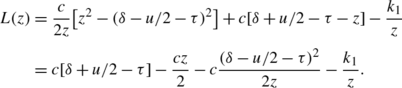
To analyze the function L(z) in interval [δ−u/2−τ,δ+u/2−τ], we compute its derivative:
$$L'(z) = c\frac{(\delta-u/2-\tau)^2}{2z^2}-\frac{c}{2} + \frac{k_1}{z^2} = \frac{(\delta-u/2-\tau)^2 + 2k_1/c - z^2}{2 z^2/c}. $$The positive solution of the derivative is \(z_{0} = \sqrt{(\delta -u/2-\tau )^{2} + 2k_{1}/c}\). Obviously, z 0>δ−u/2−τ. We shall show that z 0≤δ+u/2−τ by considering two cases:
-
τ≤u: Then c=1/u, k 1≤δ−u≤δ−τ and
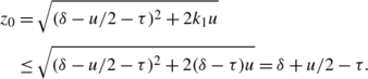
-
τ≥δ−u/2: Then c=1/(δ+u/2−τ), k 1≤δ−u, δ+u/2−τ≤u and

In both cases, function L′(z) is positive on [δ−u/2−τ,z 0], and is negative on [z 0,δ+u/2−τ]. Therefore, function L(z) is strictly increasing on [δ−u/2−τ,z 0] and strictly decreasing on [z 0,δ+u/2−τ].
Since z 0≤δ+u/2−τ, L(z 0)=c(δ+u/2−τ−z 0)≥0.
-
-
(3)
z>δ+u/2−τ: Then I 2=0 and there are two cases for computing I 1:
-
τ≤u≤δ−u/2:
$$I_1 = \frac{1}{u} \int_{\delta-u/2-\tau}^{\delta+u/2-\tau} x \,dx = \frac {1}{2u}\bigl[(\delta+u/2-\tau)^2 - (\delta-u/2- \tau)^2\bigr] = (\delta-\tau). $$The local benefit L(z) can be computed as
$$L(z) = \frac{1}{z}[\delta-\tau-k_1]. $$ -
τ≥δ−u/2:
$$I_1 = \frac{1}{\delta+u/2-\tau} \int_{0}^{\delta+u/2-\tau} x \,dx = \frac {\delta+u/2-\tau}{2}. $$The local benefit L(z) can be computed as
$$L(z) = \frac{1}{2z}[\delta+u/2-\tau-2k_1]. $$
Therefore, in both cases L(z)→0 as z→∞ and L(z) is either strictly decreasing or strictly increasing on this interval.
-


Based on the three cases, the local benefit L(z) is strictly increasing on [0,z 0] and strictly decreasing on [z 0,δ+u/2−τ] with L(z 0)≥0. Since L(z)→0 as z→∞ and L(z) is either strictly decreasing or strictly increasing on interval [δ+u/2−τ,∞), the maximum value is achieved at some point \(\hat{z} = z_{0} \in[\delta-u/2-\tau,\delta+u/2-\tau]\).
We have hence proved that if τ≤u or τ≥δ−u/2, then \(\hat{z} \in[\delta-u/2-\tau,\delta+u/2-\tau]\). To conclude the proof, we need to show that in the next step of the algorithm (at the next attacker move), the invariant that τ≤u or τ≥δ−u/2 also holds.
Assume, for simplicity, that the previous defender move before current time t (when the attacker moved) happened at time t 0<t. Then the defender’s next move t 1 is in interval [t 0+δ−u/2,t 0+δ+u/2]. The attacker receives as feedback τ=t−t 0 and his next move given by the Greedy algorithm is scheduled at time
There are two cases to consider:
-
\(t_{1} \le t+\hat{z}\) (the defender’s next move is before the attacker’s next move): Then the feedback received by the attacker at the next move is \(\tau' = t+\hat{z}-t_{1} \le(t_{0}+\delta +u/2)-(t_{0}+\delta-u/2) = u\).
-
\(t+\hat{z}< t_{1}\) (the attacker’s next move is before the defender’s next move): Then the feedback received by the attacker at the next move is \(\tau' = t+\hat{z}-t_{0} \ge\delta-u/2\).
This concludes our proof. □
Rights and permissions
About this article
Cite this article
van Dijk, M., Juels, A., Oprea, A. et al. FlipIt: The Game of “Stealthy Takeover”. J Cryptol 26, 655–713 (2013). https://doi.org/10.1007/s00145-012-9134-5
Received:
Published:
Issue Date:
DOI: https://doi.org/10.1007/s00145-012-9134-5