The Helioseismic and Magnetic Imager (HMI) Vector Magnetic Field Pipeline: SHARPs – Space-Weather HMI Active Region Patches

Abstract

A new data product from the Helioseismic and Magnetic Imager (HMI) onboard the Solar Dynamics Observatory (SDO) called Space-weather HMI Active Region Patches (SHARPs) is now available. SDO/HMI is the first space-based instrument to map the full-disk photospheric vector magnetic field with high cadence and continuity. The SHARP data series provide maps in patches that encompass automatically tracked magnetic concentrations for their entire lifetime; map quantities include the photospheric vector magnetic field and its uncertainty, along with Doppler velocity, continuum intensity, and line-of-sight magnetic field. Furthermore, keywords in the SHARP data series provide several parameters that concisely characterize the magnetic-field distribution and its deviation from a potential-field configuration. These indices may be useful for active-region event forecasting and for identifying regions of interest. The indices are calculated per patch and are available on a twelve-minute cadence. Quick-look data are available within approximately three hours of observation; definitive science products are produced approximately five weeks later. SHARP data are available at jsoc.stanford.edu and maps are available in either of two different coordinate systems. This article describes the SHARP data products and presents examples of SHARP data and parameters.

1 Introduction

This article describes a data product from the Solar Dynamics Observatory’s Helioseismic and Magnetic Imager (SDO/HMI) called Space-weather HMI Active Region Patches (SHARPs). SHARPs follow each significant patch of solar magnetic field from before the time it appears until after it disappears. The SHARP data series currently include 16 indices computed from the vector magnetic field in active-region patches. These parameters, many of which have been associated with enhanced flare productivity, are automatically calculated for each solar active region using HMI vector magnetic-field data with a 12-minute cadence. The indices and other keywords can be used to select regions and time intervals for further study. The active-region patches are automatically identified and tracked for their entire lifetime (Turmon et al. 2014). In addition to the indices, the four SHARP data series include the photospheric vector magnetic-field data for the patches, as well as co-registered maps of Doppler velocity, continuum intensity, line-of-sight magnetic field, and other quantities.

Measurements of the photospheric magnetic field provide insight into understanding and possibly predicting eruptive phenomena in the solar atmosphere, such as flares and coronal mass ejections. For example, it is generally accepted that large, complex, and rapidly evolving photospheric active regions are the most likely to produce eruptive events (Zirin 1988; Priest 1984). As such, it is an active area of research to seek a correlation (or its rejection) between eruptive events and quantitative parameterizations of the photospheric magnetic field. Many studies have found a relationship between solar-flare productivity and various indices: magnetic helicity (e.g. Tian et al., 2005; Török and Kliem, 2005; LaBonte, Georgoulis, and Rust, 2007), free-energy proxies (e.g. Moore, Falconer, and Sterling, 2012), magnetic shear angle (e.g. Hagyard et al., 1984; Leka and Barnes, 2003a, 2003b, 2007), magnetic topology (e.g. Cui et al., 2006; Barnes and Leka, 2006, Georgoulis and Rust, 2007), or the properties of active-region polarity-inversion lines (e.g. Mason and Hoeksema, 2010; Falconer, Moore, and Gary, 2008; Schrijver, 2007). However, when Leka and Barnes (2003a) conducted a discriminant analysis of over a hundred parameters calculated from vector magnetic-field measurements of seven active regions, they could identify “no single, or even small number of, physical properties of an active region that is sufficient and necessary to produce a flare.” Larger statistical samples show correlations between some vector-field non-potentiality parameters and overall flare productivity (Leka and Barnes 2007; Yang et al. 2012), as well as correlations between the parameters themselves. Still, characteristics have yet to be identified that uniquely distinguish imminent flaring in an active region.

The SHARP data series will provide a complete record of all visible solar active regions since 1 May 2010. SHARP data are stored in a database and are readily accessible at the Joint Science Operations Center (JSOC). JSOC data products from SDO, as well as source code for the modules, can be found at jsoc.stanford.edu . Continuously updated plots of near-real-time parameters are available online (see Table 1 for URLs). We describe how the SHARP series are created and show results for two representative active regions. We also present examples of four active-region parameters for 12 X-, M-, and C-class flaring active regions.

Table 1 Listed below are URLs relevant for finding the SHARP data, codes, documentation, and data visualizations. These URLs will be maintained for at least the duration of the SDO mission.

2 Methodology: SHARP Data and Active Region Parameters

Data taken onboard SDO/HMI are downlinked to the ground, automatically processed through the HMI data pipeline, and made available at jsoc.stanford.edu organized in data series (Schou et al. 2012a; Scherrer et al. 2012). Conceptually, a JSOC data series consists of a sequence of records, each of which includes i) a table of keywords and ii) associated data arrays, called segments. A record exists for each time step or unique set of prime keyword(s). Keywords and data-array segments are merged by the JSOC into FITS files in response to a user’s request to download (or export) the data series. SHARP data for export can be selected by time, given in the keyword t_rec, and the region number harpnum; additionally, requests for data from the JSOC can also take advantage of simple SQL database queries on keywords to select data of interest. A complete overview of JSOC data series is available on the JSOC wiki (see Table 1). Certain HMI data series are processed on two time scales: near-real-time (NRT) and definitive. NRT data are processed quickly, ordinarily within three hours of the observation time, but with preliminary calibrations. Section 7 describes the differences between definitive and NRT SHARPs. Although most NRT data series are not archived and go offline after approximately three months, the NRT SHARP data since 14 September 2012 are archived. NRT data are primarily intended for quick-look monitoring or as a forecasting tool. This section briefly describes the elements of the HMI data pipeline necessary to create the definitive SHARP data. A more detailed explanation of the HMI vector magnetic-field pipeline processing is given by Hoeksema et al. (2014) and references therein.

• In each 135-second interval, HMI samples six points across the Fe i 6173.3 Å spectral line and measures six polarization states: I±Q, I±U, and I±V, generating 36 4096 × 4096 full-disk filtergrams.

• To reduce noise and minimize the effects of solar oscillations, a tapered temporal average is performed every 720 seconds using 360 filtergrams collected over a 1350-second interval to produce 36 corrected, filtered, and co-registered images (Couvidat et al. 2012).

• A polarization calibration is applied and the four Stokes polarization states [I  Q  U  V] are determined at each wavelength, giving a total of 24 images at each time step (Schou et al. 2012b), which are available in the data series hmi.S_720s.

• Active-region patches are automatically detected and tracked in the photospheric line-of-sight magnetograms (Turmon et al. 2014). The detection algorithm identifies both a rectangular bounding box on the CCD image that encompasses the entire region and, within this box, creates a bitmap that both encodes membership in the coherent magnetic structure and indicates strong-field pixels. Specifically, the bitmap array assigns a value to each pixel inside the bounding box, depending on whether it i) resides inside or outside the active region, and ii) corresponds to weak or strong line-of-sight magnetic field. This coding scheme permits non-contiguous active-region patches.

• The tracking module numbers each HMI Active Region Patch (HARP) and generates a time series of bitmaps large enough to contain the maximum known heliographic extent of the region. Each numbered HARP (keyword harpnum) corresponds to one active region or AR complex (see Figure 1). The HARP database generally captures more patches of solar magnetic activity than the NOAA active-region database because coherent regions that are small in extent or have no associated photometric sunspot are detected and tracked by our code; such faint HARPs often have no NOAA correspondence. A HARP may include zero, one, or multiple NOAA active regions (for example, see HARP 2360 in Figure 1); about one-third of HARPs correspond to a single NOAA region. The bitmap array described above is in the bitmap segment of the data series hmi.Mharp_720s. The terms HARP and SHARP are not quite interchangeable. The HARP data series primarily provides geometric information about the patch. The SHARP also includes cut-outs of the observables and computed indices.

  Figure 1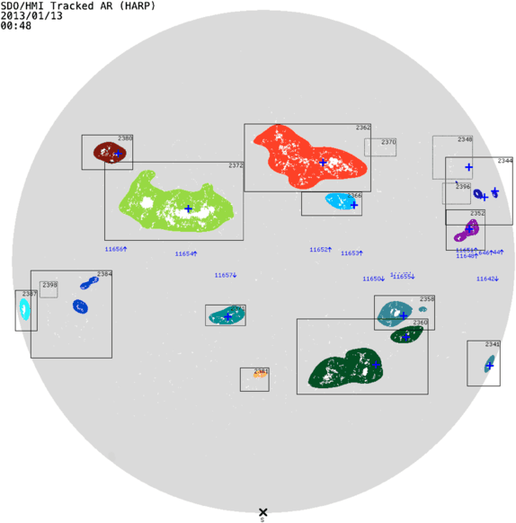

  

  The results of the active-region automatic detection algorithm applied to the data on 13 January 2013 at 00:48 TAI. NOAA active-region numbers are labeled in blue near the Equator, next to arrows indicating the hemisphere; the HARP number is indicated inside the rectangular bounding box at the upper right. Note that HARP 2360 (lower right, in green) includes two NOAA active regions, 11650 and 11655. The colored patches show coherent magnetic structures that comprise the HARP. White pixels have a line-of-sight field strength above a line-of-sight magnetic-field threshold (Turmon et al. 2014). Blue ‘+’ symbols indicate coordinates that correspond to the reported center of a NOAA active region. The temporal life of a definitive HARP starts when it rotates onto the visible disk or two days before the magnetic feature is first identified in the photosphere. As such, empty boxes, e.g. HARP 2398 (on the left), represent patches of photosphere that will contain a coherent magnetic structure at a future time.

• The full-disk Stokes data are inverted using the Very Fast Inversion of the Stokes Vector (VFISV) code, which assumes a Milne–Eddington model of the solar atmosphere, to yield vector magnetic field data (Borrero et al. 2011; Centeno et al. 2014). Inverted data are available in the data series hmi.ME_720s_fd10. Full-disk inversions are being computed for all HMI data since 1 May 2010. An improvement made to the inversion code in May 2013 (Hoeksema et al. 2014) to use time-dependent information about the HMI filter profiles introduces measurable systematic differences in inversion results. Data in the interval from 1 August 2012 – 24 May 2013 were processed before the improvement. Some care must be taken when comparing data computed with different versions of the analysis code (see the entry under PipelineCode referenced in Table 1).

• The azimuthal component of the vector magnetic field is disambiguated using the Minimum Energy Code (ME0) to resolve the 180^∘ ambiguity (Metcalf 1994; Leka et al. 2009). Through 14 January 2014 SHARP regions have been disambiguated individually using fd10 data inside a rectangle that extends beyond the HARP bounding box by the number of pixels given in the ambnpad keyword. Disambiguation results for each harpnum at each time step are stored in the disambig segment of the hmi.Bharp_720s data series. All pixels inside the rectangular bounding box are annealed in the patchwise SHARP disambiguation; however, pixels below a noise threshold are also smoothed (Barnes et al. 2014; Hoeksema et al. 2014). Since 19 December 2013 we have disambiguated the entire disk and use that data set from the consistently derived disambig segment of the hmi.B_720s data series for definitive SHARPs observed from 15 January 2014 onward.

• Finally, to complete the SHARP data series the analysis pipeline collects maps of HMI observables and computes a set of active-region summary parameters using a publicly available module (see Table 1 and Section 4).

3 SHARP Coordinates: CCD Cutouts and Cylindrical Equal-Area Maps

HMI data series use standard World Coordinate System (WCS) for solar images (Thompson 2006). SHARP data series are available in either of two coordinate systems: one is effectively cut out directly from corrected full-disk images, which are in helio-projective Cartesian CCD image coordinates, and the other is remapped from CCD coordinates to a heliographic Cylindrical Equal-Area (CEA) projection centered on the patch. Table 2 lists the four available SHARP data series.

Table 2 Four series that contain SHARP data. SHARP active-region parameters are stored as keywords for these series. For a list of parameters, see Table 3.

For standard CCD-cutout SHARPs, the pipeline module collects 31 maps, including many of the primary HMI observable data segments (line-of-sight magnetogram, Dopplergram, continuum intensity, and vector magnetogram), other inversion and disambiguation quantities, uncertainty arrays, and the HARP bitmap. Using the HARP bounding box as a stencil, the module extracts the corresponding arrays of observable data. The first six tables in the Appendix give a description of each of the cut-out SHARP series segment maps.

Additional processing is applied to the CEA versions of the SHARPs to convert selected segments from CCD pixels in plane-of-the-sky coordinates to a heliographic coordinate system in the photosphere. Table A.7 in the Appendix lists the 11 segment maps that are available in CEA coordinates.

The expression relating the final CEA map coordinate [x,y] to the heliographic longitude and latitude [ϕ,λ] follows Equations (79) and (80) of Calabretta and Greisen (2002), compliant with the World Coordinate System (WCS) standard (e.g. Thompson, 2006). The remapping uses the patch center as reference point, thus effectively de-rotating the patch center to ϕ=0, λ=0 before CEA projection to minimize distortion (see Section 2.5 of Calabretta and Greisen, 2002). As a consequence, the correspondence between what are labeled CEA degrees and the familiar Carrington latitude and longitude is complex. The Carrington coordinates of the patch center are indicated in the keywords crval1 and crval2. The SHARP CEA pixels have a linear dimension in the x-direction of 0.03 heliographic degrees in the rotated coordinate system and an area on the photosphere of 1.33×10⁵ km². The size in the y-direction is defined by the CEA requirement that the area of each pixel be the same, so the pixels are equally spaced in the sine of the angular distance from the great circle that defines the x-axis, and the step size is fixed such that the pixel dimension is equal to 0.03 degrees at patch center. In Figures 2 and 3 the axes are labeled in CEA degrees with the center point having the Carrington longitude and latitude values. In our remapping process the CEA grid is oversampled by interpolating the nearby CCD values and then smoothed with a Gaussian filter to the final sampling. Details are provided by Sun (2013).

Figure 2

The first three panels, clockwise from upper left, show the inverted and disambiguated data wherein the vector B has been remapped to a Cylindrical Equal-Area projection and decomposed into B _r , B _θ , and B _ϕ , respectively, for HARP 401 (NOAA AR 11166) on 9 March 2011 at 23:24:00 TAI. The color table is scaled between ± 2500 Gauss for all three magnetic-field arrays. The lower-left panel shows the computed continuum intensity for the same region at the same time. The patch is centered on longitude 90.91^∘, latitude 9.59^∘ in Carrington Rotation 2107. CEA longitude and latitude are described in the text.

Figure 3

Only pixels that are both within the HARP (shaded orange in map segment bitmap, upper left) and above the high-confidence disambiguation threshold (shown in white in the upper right panel where segment conf_disambig = 90) contribute to the active-region parameters (represented in the bottom panel). This example from hmi.sharp_720s_cea shows HARP 401 (NOAA AR 11166) on 9 March 2011 at 23:24:00 TAI, where the quantities have been remapped to a Cylindrical Equal-Area coordinate system. Black areas at the edge of the bitmap and conf_disambig images fall outside the maximal CCD HARP bounding box; therefore, the azimuthal ambiguity resolution has not been applied to these areas. As in Figure 2, the axes are labeled in CEA coordinates, as described in the text.

The remapping of the uncertainty images, as well as the bitmap and conf_disambig maps, is done a little differently. For these the center of each pixel in the remapped CEA coordinate system is first located in the original CCD image; then the nearest neighboring pixel in the original image is identified, and the value for that nearest original CCD pixel is reported.

For the CEA version, the native three-component vector magnetic-field output from the inversion – expressed as field strength [B], inclination [γ], and azimuth [ψ] in the image plane – is transformed into the components B _r , B _θ , and B _ϕ in standard heliographic spherical coordinates $[\hat{\boldsymbol{e}}_{r}, \hat{\boldsymbol{e}}_{\theta}, \hat{\boldsymbol{e}}_{\phi}]$ following Equation (1) of Gary and Hagyard (1990). Figure 2 shows the three components of the vector magnetic field and the computed continuum intensity for HARP 401 on 9 March 2011 at 23:24 TAI in CEA coordinates. We note that because $(\hat{\boldsymbol{e}}_{r}, \hat{\boldsymbol{e}}_{\theta}, \hat{\boldsymbol{e}}_{\phi})$ is a spherical coordinate system with the rotation axis at the pole and $(\hat{\boldsymbol{e}}_{x}, \hat{\boldsymbol{e}}_{y}, \hat{\boldsymbol{e}}_{z})$ is a planar cylindrical equal-area coordinate system centered on the patch, the unit vectors $(\hat{\boldsymbol{e}}_{\theta}, \hat{\boldsymbol{e}}_{\phi})$ do not precisely align with $(\hat{\boldsymbol{e}}_{x}, \hat{\boldsymbol{e}}_{y})$ except at the center of the patch. In general, only along the y-axis passing through patch center do $\hat{\boldsymbol{e}}_{\phi}$ and $\hat{\boldsymbol{e}}_{y}$ align. See Figure 2 of Calabretta and Greisen (2002) for an illustrative example. For more information on SHARP coordinate systems, mapping, and vector transformations, see Sun (2013).

4 SHARP Summary Parameters

The SHARP module calculates summary parameters every twelve minutes on the inverted and disambiguated data using the vector field and other quantities in the CEA projection. The SHARP series currently contain sixteen summary parameters, as detailed in Table 3. This initial list parametrizes some of the features of solar active regions that have been associated with enhanced flare productivity (e.g. Leka and Barnes, 2003a, 2007, and references therein) and includes different kinds of indices such as the total magnetic flux, the spatial gradients of the field, the characteristics of the vertical current density, current helicity, and a proxy for the integrated free magnetic energy. Until now, indices based on vector-field values have not been available with the coverage, cadence, and continuity afforded by HMI. With previously available data, none of the parameters were found to be necessary or sufficient to forecast a flaring event (Leka and Barnes 2007). As of this writing, the SHARP indices focus on low-order statistical moments of observables and readily derived quantities. As the SHARP database develops further, new quantities will be added, including ones that characterize the magnetic-inversion lines, the relevant fractal indices, and models of the coronal field (see Section 9 for further discussion).

Table 3 Active-region parameters are stored as keywords in each SHARP series. This table lists each active-region parameter keyword with a brief description and formula. The keyword for the error associated with each parameter is given in the last column. Each parameter represents either a mean, sum, or integral of the distribution in the high-confidence part of the HARP; this is indicated in the Statistic column. The active-region parameters were generally adapted from Leka and Barnes (2003b) except as noted in the text. WCS-standard keywords such as cdelt1, rsun_obs, and rsun_ref, as well as fundamental constants, were used to convert to the units specified in the eponymous column. Calculations are performed on the cmask high-confidence pixels in the CEA SHARP. Derivations of the errors can be found at the SHARP web page (see Table 1). Further description of the parameters can be found in Section 5.

The pixels that contribute to any given index calculation are selected by examining two data segment maps: bitmap and conf_disambig. The bitmap segment, an example of which is shown in the upper left panel of Figure 3, identifies pixels within the HARP (bitmap ≥ 33). Pixels with strong line-of-sight magnetic-field strength are shown in white, whether inside or outside the orange HARP area. The conf_disambig segment has a high value for clusters of pixels above the spatially and temporally dependent disambiguation noise threshold (≈ 150 G, conf_disambig = 90; see Table A.5 and Hoeksema et al., 2014). Only data that are both within the HARP and above the high-confidence threshold contribute to the SHARP parameter calculation; the number of contributing CEA pixels is given in the keyword cmask. The bottom panel of Figure 3 shows the pixels that contribute to the active-region parameters for HARP 401 (NOAA AR 11166) on 9 March 2011 at 23:24:00 TAI. The indices in all four SHARP series are computed from the CEA data.

5 SHARP Parameters for an Illustrative Region: HARP 401

The SHARP indices are common active-region parameters described in the literature, as discussed in the previous section, and the formulae are given in Table 3. Figures 4 and 5 show the SHARP indices for HARP 401 from the time it first rotated onto the disk on 2 March 2011 through its final disappearance on 15 March. Computed quantities from Table 3 are plotted with error bars, except for those that are areas or pixel counts. In most cases the error bars are smaller than the size of the dots, because formal errors are small and systematic errors are not reflected. We have excluded data points with poor status bits set in the quality keyword, which provides information about data reliability (see Table A.8 and Lev1qualBits referenced in Table 1 for more information about quality).

Figure 4

SHARP active-region parameters for HARP 401, 2 – 15 March 2011. Column A on the left shows four quantities: Panel A1, area; A2, cmask; A3, area_acr; and A4, usflux; Column B on the right shows five quantities: Panel B1, meangam; B2, meanshr; B3, shrgt45; B4, meanpot; and B5, meanjzd.

Figure 5

Additional SHARP active-region parameters for HARP 401, 2 – 15 March 2011. Column A on the left shows five quantities: Panel A1, totusjh; A2, totpot; A3, totusjz; A4, meangbt; and A5, meangbh. Column B on the right shows five quantities: Panel B1, meanjzh; B2, absnjzh; B3, savncpp; B4, meanalp; and B5, meangbz.

The photospheric area (Figure 4 Panel A1, top left) is determined by the HARP module using the HMI line-of-sight magnetic field measurements. The area includes everything inside the orange patch in the upper left panel of Figure 3. This established active region rotates onto the disk on 2 March and grows steadily as it crosses the disk. The patch reaches a maximum area of ≈ 7500 microhemispheres on 11 March before it starts to decrease as it rotates off the disk. The panel below (Figure 4 Panel A2) shows the total number of high-confidence pixels that contribute to the SHARP index calculation [cmask], i.e. the pixels in white in the bottom panel of Figure 3. Once the region is on the disk, the number of cmask pixels increases from about 40 000 to nearly 80 000. The number of contributing pixels changes with the size of the region and also depends on the noise threshold that varies with location on the disk and velocity of SDO relative to the Sun (see Section 7.1 of Hoeksema et al., 2014). A histogram of the total-field noise level (not shown) increases and broadens near 60^∘ from central meridian, consequently increasing the number of pixels above the noise threshold relative to disk center.

For comparison, Figure 4 Panel A3 shows the area of the strong active pixels determined from the line-of-sight field during the initial identification of the HARP region. This area [area_acr] associated with the white pixels inside the orange patch on the upper left of Figure 3, is smaller than the area associated with the high-confidence pixels in the center panel of that figure. The area of strong field shows a steady 40 % increase during the new flux emergence on 7 – 8 March. The total unsigned flux [usflux] computed from the radial component of the vector magnetic field appears in Figure 4 Panel A4, at the bottom of the left column. The total flux, initially about 3×10²² Mx, decreases by 20 % on 6 March, recovers by a similar amount late on 7 March, and then gradually builds to about 5×10²² Mx on 13 March. Variations in usflux in this time interval do not exactly track changes in the area of the region, the number of pixels in the computation, or the strong-pixel area, indicating that the strength of the field in the region is also changing. Correlated daily variations in usflux and cmask are associated with SDO’s geosynchronous orbital velocity. The episode of flux emergence during 7 and 8 March is reflected in a number of the quantities. The largest flare produced by HARP 401, an X 1.5 flare, peaked at 23:23 TAI on 9 March, about the time that the active-pixel area first reaches a maximum. Numerous C-class and M-class flares occurred during the lifetime of the region.

The systematic change in the transverse-field noise level is reflected in the trend of the mean value of the inclination angle [meangam] shown in Panel B1 at the top right of Figure 4. The plot shows both the evolution of the region and a position-dependent trend that results from the different strengths and noise levels in the circular and linear polarization signals. (See Borrero and Kobel (2011) for a relevant discussion of the effects of noise on the interpretation of vector-field measurements.) At disk center, the vertical magnetic-field component [B _z ] is closest to the lower-noise line-of-sight direction that depends on the stronger Stokes-V; the horizontal component [B _h] reflects the sensitivity to noise in Stokes-Q and -U. In weak-field pixels this tends to bias the inclination angle away from 0^∘. The relative contributions of noise to the vertical- and horizontal-field components change with center-to-limb angle [μ]. As a consequence, the ratio B _z /B _h in the weak-field pixels increases, decreasing the horizontal bias in the reported inclination. meangam reaches a maximum of ≈ 60^∘ from radial near disk center and shows two broad minima at 45^∘ and 40^∘ when the region is near the east and west limbs, respectively, where the noise contributions to the vertical and horizontal field components are roughly the same.

The mean shear angle [meanshr] in Figure 4 Panel B2 shows a similar variation across the disk, with a maximum a little over 50^∘ near central meridian passage and broad minima below 40^∘ and 35^∘ in the East and West, respectively. The shear angle is calculated by determining the angle between the observed field [B ^Obs] and a potential field [B ^Pot]. To compute the parameters that require a potential-field model, we used the discretized Green’s function based on Equation (2.14) of Sakurai (1982), which is the potential due to a submerged monopole at a depth of $\Delta/\sqrt{2\pi}$. In that case, Δ is the size of a pixel, which preserves the total flux of B _z . However, using that depth yields a B _z map that is blurry compared with the original observational data, which, in turn, yields blurry calculated B _x and B _y maps. Therefore, we chose a smaller Δ that corresponds to 0.001 pixels. Since this yields a sharper B _z map, with a resolution similar to the original observational data, the calculated B _x and B _y maps are of a higher resolution as well. We preserved the original observational data for the z-component of the potential magnetic field. Figure 4 Panel B3, the fraction of cmask pixels with shear greater than 45^∘ [sheargt45], shows a pattern very similar to the mean shear and mean inclination angle. Trends in the large-scale averages are affected by what is happening in the weak and intermediate field-strength pixels near the noise level and the systematic change in reported field direction from center to limb. There is a few percent decrease in the fraction of strong-shear pixels over the course of 9 March, prior to the X-class flare, which may or may not be significant.

Figure 4 Panel B4 presents the mean value of the free-energy density averaged over the patch [meanpot]. meanpot shares evolutionary characteristics of the shear and inclination angle. Figure 4 Panel B5 (bottom right) shows the evolution of the mean vertical-current density [meanjzd]. The point-to-point scatter and the uncertainties in this quantity are relatively larger than for most of the other SHARP parameters. The mean vertical-current density more than doubles from about 0.1 to 0.25 mA m⁻² on 7 March when new flux began to rapidly emerge. The vertical current is computed using derivatives of the horizontal magnetic-field components. To compute any of the parameters that require a computational derivative, we used a second-order finite-difference method with a nine-point stencil centered on each of the cmask pixels.

We now consider Figure 5, which shows additional SHARP parameters for the same HARP 401. Figure 5 Panels A1 and A2 on the upper left show the total unsigned current helicity [totusjh] and a proxy for the integrated total free-energy density [totpot]. Both quantities show a sustained increase on 7 March when new flux was emerging. The total current helicity showed a sharp increase from 3100 to 3900 G² m⁻¹ on 9 March leading up to the X-class flare. The integrated free-energy density is the difference between the observed and potential magnetic-field energy integrated over the region. totpot nearly doubles from 5×10²³ to 9×10²³ erg cm⁻¹ on 7 March; however, no obvious signal associated with the flare or its immediate aftermath is reflected in the free-energy density plot. In fact, totpot continues to increase gradually until 11 March.

The total unsigned vertical current (totusjz in Figure 5 Panel A3) changes dramatically during the life of HARP 401. Like the current helicity and integrated free-energy density, it reaches a plateau on 5 March and then increases rapidly on 7 and 8 March from 4×10¹³ to 7×10¹³ A. A dip and rapid rise occur on 9 March before the X-class flare, after which the current stabilizes for several days.

Figure 5 Panels A4, A5 (bottom left), and B5 (bottom right) show the temporal dependence of the horizontal gradients of the field. Each index is the mean value of the gradient computed at the cmask pixels in the patch. Figure 5 Panel A4 shows the mean horizontal gradient of the total field magnitude [meangbt]. There is a fairly clear daily periodicity associated with the spacecraft velocity and the number of pixels in cmask. The daily variation is superposed on a broad peak near central meridian at about 100 G Mm⁻¹. The same shape is evident in Figure 5 Panel A5, which shows the horizontal gradient of the horizontal component of the field [meangbh]. The peak is a little sharper, ranging from ≈ 20 – 65 G Mm⁻¹ during the disk passage of the region. Figure 5 Panel B5 (on the lower right) shows that the horizontal gradient of the vertical component of the field [meangbz] is less sharply peaked near central meridian and has a more pronounced daily variation. Consideration of other regions (see the discussion of HARP 2920 and Figure 6) suggests that the broad shape tends to follow that of cmask and area; so, perhaps the mean gradient of the vertical field is more heavily influenced by the contributions of the variable number of weak-field pixels than are the means of the total or horizontal field gradient.

Figure 6

SHARP active-region parameters for HARP 2920, 1 – 14 July, 2013. Column A on the left shows four quantities: Panel A1, cmask; A2, acr_area; A3, usflux; and A4, totusjz. Column B on the right shows four quantities: Panel B1, meangam; B2, absnjzh; B3, meanpot; and B4, meangbt.

Figure 5 Panel B1 (upper right) shows the mean of the contribution to the current helicity from the vertical components of the magnetic field and the current density [meanjzh]. We cannot calculate the other terms that contribute to the total helicity because HMI cannot determine the field gradient in the vertical direction. The mean current helicity is generally negative for this region through much of its lifetime and shows relatively strong variability while the region is evolving rapidly from 6 – 11 March. Starting 12 March, the helicity was relatively large in magnitude, at −0.004 G² m⁻¹, but stable. Indices plotted in the next three panels, B2, B3, and B4, are related to physical quantities associated with helicity, and thus all share a similar temporal profile. The sum of the absolute values of the net current helicity [absnjzh] is shown in Figure 5 Panel B2; the sum of absolute values of the net current determined separately in the positive and negative B _z regions [savncpp] appears in Figure 5 Panel B3; and the mean of the magnetic-field twist [α] of the region [meanalp] is in Figure 5 Panel B4. All exhibit some degree of daily variation. Periodic variations are particularly strong on 6, 7, 9, and 11 March. All experience a steep increase in magnitude on 11 – 12 March, after which the indices remain fairly stable. The sum of the net currents in the two polarity regions [savncpp] peaks above 2×10¹³ A on 13 March.

The average twist parameter [meanalp] posed a challenge. The simple definition of twist [α=J _z /B _z ] is noisy for individual pixels when the field is low and near the noise level (cf. Leka and Skumanich, 1999). Simply averaging the computed α in the high-confidence SHARP region pixels results in a meaningless scatter of points from one time step to the next, suggesting that a higher threshold may be more appropriate. Instead we calculated a parameter intended to reflect the mean twist of the field in the entire active region. A variety of methods have been proposed (Pevtsov, Canfield, and Metcalf 1995; Leka et al. 1996; Leka and Skumanich 1999; Falconer, Moore, and Gary 2002) based on fits to differences from a linear force-free field, moments of the distribution of α, and taking ratios of spatial averages determined in parts of the active region. None of the methods is clearly superior. For the SHARP index meanalp we adopted the $B_{z}^{2}$-weighted α method proposed by Hagino and Sakurai (2004) in which one simply computes the sum of the product of J _z B _z at the cmask pixels and divides by the sum of $B_{z}^{2}$.

6 Selected Parameters for a Second Region: HARP 2920

Considering a single active-region complex does not provide sufficient context to understand how regions differ from each other or how much of the variation in a quantity depends on disk position or other typical evolutionary characteristics. To illustrate the differences between regions, Figure 6 shows selected SHARP indices for HARP 2920 from the time that it first rotated onto the disk on 1 July 2013 through its final disappearance on 14 July. HARP 401 was energetic and large, but had reasonably simple large-scale topology. HARP 2920 was larger and more complex, ultimately including three NOAA regions: 11785, 11787, and 11788. HARP 2920 produced numerous C-class flares; the largest, class M 1.5, occurred at 07:18 UT on 3 July while the region was still near the east limb. Figure 6 Panel A1 (cmask, upper left) shows the number of high-confidence CEA pixels that contribute to the indices. Panel A2 shows the area associated with strong pixels [area_acr]. The region grows as it rotates onto the disk, and then on 3 and 4 July its size nearly doubles from about 1400 microhemispheres on 2 July to 2100 on 3 July, as a second activity complex (AR 11787) rotates over the limb, and then to 2800 by the end of 4 July as new flux emerges. In the NRT HARP this appearance and nearby emergence results in the merger of two regions. The size of the region remains fairly stable as it continues to rotate across the disk. The active pixel area [area_acr] starts to diminish on 10 March, but the size of the high-confidence pixel area [cmask] only begins to decrease rapidly starting on 12 July as the HARP rotates off the limb. Compare this with the strong emergence of new flux within the existing flux system seen in HARP 401 on 8 – 9 July.

The evolution of the total unsigned flux [usflux] appears in Figure 6 Panel A3. The change in cmask pixel number creates broad peaks near 60^∘ from central meridian on 4 July and 12 July in the usflux. The variations of cmask and usflux were also correlated for HARP 401, but the evolution across the disk was very different. The trend also seems to be reflected in an inverse fashion in the mean inclination angle [meangam] plotted in Figure 6 Panel B1 (top right). A similar inverted trend appears, with a broad peak near central meridian on 8 – 9 July, in the measures of shear angle and the mean vertical-current density (not shown). The similarity of the meangam profile for 401 and 2920 confirms that significant effects due to the relative noise levels in Stokes Q, U, and V are important.

Figure 6 Panel B2 shows the modulus of the net current helicity [absnjzh]. There is a strong rise on 2 – 4 July and again on 5 July followed by a sharp decline on 6 and 7 July. The mean-current-helicity, net-current-per-polarity, and mean-twist parameters (not shown) have a similar profile. Compare this with the weaker and relatively less volatile behavior of HARP 401 (note the difference in plot scale) even though 401 was emerging much more new flux. The mean free-energy density [meanpot, Figure 6, Panel B3] remains fairly stable at 7000 ergs cm⁻³ from the time the region appeared until a steady decrease begins on 9 July. The mean free-energy density of HARP 401 was significantly greater and increased by ≈ 30 % during its disk passage before beginning a similar decline. The variations of the total unsigned vertical current [totusjz, Figure 6 Panel A4] are representative of the total unsigned current helicity and integrated free-energy density proxy. Unlike HARP 401, these quantities in HARP 2920 do not follow the evolution of the unsigned flux or the area. There is an interesting small excursion in the vertical current on 6 July just after the helicity measures reach their peak and begin their rapid decline. No similar relationship is seen in HARP 401.

Finally, Figure 6 Panel B4 plots the mean of the horizontal gradient of the total field strength [meangbt], which is indicative of the evolution of the mean gradients of the other field components. The broad hump on the meangbt curve that occurs on 9 – 10 July is not apparent in any of the indices unrelated to field-strength gradients. Otherwise the evolution is very smooth, much smoother than for HARP 401. All gradient indices exhibit a short-term (12-hour) variation that is related to the sensitivity of the vector-field measurement to the orbital velocity of the spacecraft (Hoeksema et al. 2014). The general profile of the mean gradient of the horizontal-field component (not shown) for HARP 2920 has a broad peak near central meridian passage, as does the area of the strong-field elements. The mean gradients of the total and vertical field (not shown) follow the flatter shape of the total area more closely, with additional broad increases appearing near 60^∘ from central meridian associated with the increase in the number of weak- and intermediate-strength pixels, although both start to decrease steadily on 10 July.

7 Definitive and Near-Real-Time (NRT) SHARPs

The definitive HARP processing module groups and tailors the identified regions according to their complete life history. The definitive HARP geometry is determined only after an active-region patch has crossed the face of the disk. At each time step the rectangular bounding box of a definitive HARP on the CCD encloses the fixed heliographic region that encompasses the greatest geometric extent attained by the patch during its entire lifetime. The temporal life of a definitive HARP starts when it rotates onto the visible disk or two days before an emerging magnetic feature is first identified in the photosphere. The HARP expires two days after the feature decays or when it rotates completely off the disk. The center of the HARP at central meridian passage is uniformly tracked at the differential-rotation rate appropriate for its latitude, given in keyword omega_dt. There is necessarily a delay of about five weeks before definitive SHARPs can be created.

Operational space-weather forecasting requires more timely data and would need to rely on the HMI NRT data stream. We outline below three primary differences between the NRT data and definitive SHARP data. Note that the harpnum for a particular region will be different for the definitive and NRT SHARP series. The NRT SHARPs are offered “as is”; i.e. there is no plan to necessarily correct the NRT data series when updates are made to the definitive SHARPs. The NRT SHARP archive begins 14 September 2012, but because of the inferior quality of the NRT data, we strongly recommend against use of the NRT data except for forecasting and development of forecasting tools.

• i) The NRT and definitive observables input data differ in completeness and calibration. Roughly 4 % of the data are delayed more than one hour; delays tend to be more clustered than random. Calibrations and corrections to the NRT data rely on predicted conditions or on calibration information that may be increasingly out of date as the day progresses. Effects of cosmic rays are not corrected. The differences are generally minor or localized. For a detailed summary of calibration procedures and the differences between the NRT and definitive input data, see Hoeksema et al. (2014).

• ii) NRT HARP geometry is determined as soon as possible, before the full life-cycle of the region is known. For that reason the photospheric area enclosed by the box bounding the active region can grow (but will never shrink) with time. In addition, the heliographic center of the NRT HARP bounding box may shift in time as a region evolves. In general, the size and shape of the patch itself is the same in NRT and definitive HARPs. It is important to note that NRT HARPs may merge, resulting in the termination of one HARP and the continuation of another HARP, but augmented by the content of the terminated HARP. This will typically cause a major discontinuity in the NRT SHARP indices at that time step. The h_merge keyword is set when such a merge occurs, so that merging can be taken into account when the discontinuities are observed. The h_merge keyword is also carried over into the definitive HARPs, but in this case the region configuration is consistent before and after the merge (the entire future of all regions is available), so for definitive HARPs, the relic h_merge keyword is not particularly significant. At least one merger occurred during the lifetime of 494 of the first 3213 HARPs. Note again that the NRT and definitive harpnum will not be the same.

• iii) For NRT processing, the annealing parameters for the disambiguation code are adjusted to enable faster computation (Barnes et al. 2014) and a smaller buffer outside the HARP is used to compute the potential-field starting point. The keyword ambnpad gives the size of the buffer and is reduced to 50 currently for NRT SHARPs from the 500 used for definitive processing. To investigate how these input parameters affect the active-region indices, we disambiguated a five-day cube of inverted data for HARP 401 using the two different sets of disambiguation parameters. The resulting active-region indices generally differ by less than a percent. For example, the typical difference in the total field gradient was less than 0.05 % with a maximum difference of 0.3 %. Starting on 15 January 2014, the definitive SHARPs rely on full-disk rather than patch-wise disambiguation.

Hoeksema et al. (2014) presented a detailed comparison between the definitive and quick-look total unsigned flux parameter for SHARP 2920 and found that the typical difference is about 1 % (see their Figure 5). The differences have some systematic periodic components, most likely attributable to differences in calibration. The differences increase to a few percent when SHARPs are near the limb. By far the largest difference (≈ 30 %) is due to a merger.

8 Sources of Uncertainty

The vector-magnetogram data used in this study have uncertainties and limitations that were discussed at length by Hoeksema et al. (2014). Many of these issues are more significant in weak-field regions, which do not contribute directly to the computation of active-region parameters, except that in intermediate field-strength regions near the noise threshold the number of pixels can change appreciably. Systematic errors remain, the largest are associated with the daily variation of the radial velocity of the spacecraft inherent to the geosynchronous orbit (e.g. small periodic variations in Figures 4 – 7). For each index we characterize the formal random error in the computed active-region parameter. The inversion code provides estimates of uncertainties at each pixel, including χ ², the computed standard deviations, and certain correlation coefficients of the errors in the derived parameters. They effectively provide a way to estimate a lower limit on the uncertainties. We use the uncertainty determined for each component of the vector magnetic field and formally propagate these error estimates per pixel per unit time per quantity for each SHARP index. The uncertainty keyword is listed in the last column of Table 3. To test the results, we verified our formal error propagation at a relatively early stage in the vector field pipeline using a Monte Carlo analysis in which we varied the input Stokes parameters according to the error estimates. The variability found in the final SHARP indices is consistent with the formal error propagation results.

Figure 7

Clockwise from top left, temporal profiles of the total unsigned flux [usflux], the modulus of the net current helicity [absnjzh], the mean value of the inclination angle [meangam], and the integrated total free-energy density per active region [totpot]. The entire sample is color coded: active regions associated with X-class flares are represented with red-purples, M-class by blue-greens, and C-class by yellow-browns. For clarity a larger symbol is plotted every three hours, i.e. every 15th point. The legend is in the top-left panel. The time profiles are adjusted to align the flare peaks shortly after the start of Day 5, as denoted by the red dotted–dashed line. Error bars are plotted for all points; however, in most cases, they are smaller than the point size. Scatter in the active-region parameters for NOAA AR 11429 for a few points following the flare peak is due to poor data quality following an eclipse: thermal changes in the HMI front window affect the focus. Periodicities in some of the parameters, most prominently in some temporal profiles of unsigned flux, are systematic effects due to the daily variation of the radial velocity of the spacecraft inherent to the geosynchronous orbit.

9 Sample Data and Discussion

For illustrative purposes, Figure 7 shows the evolution of a few SHARP parameters for selected active regions associated with X-, M-, and C-class flares (Table 4). A more complete analysis with comprehensive statistics is left for a future publication. Region selection was based on the following criteria: i) to minimize the effects of the increased noise in limb-ward data, we required that (a) the active region must be within 45 degrees of central meridian during the GOES X-ray flux peak, and (b) for active regions that produced multiple flares, we chose the flare that occurred while the region was closest to disk center. ii) In some cases the identification and extraction algorithm (Turmon et al. 2014) identifies as one coherent magnetic structure – i.e., one HARP – a region associated with multiple NOAA active regions. For simplicity, such HARPs were excluded from this sample. iii) To make a good comparison we identified the largest class of flare associated with each active region. Thus a C-class region would not have produced any M- or X-class flares. For each flare class we then arbitrarily selected just four regions to show in Figure 7 as a demonstration of the currently available SHARP parameters.

Table 4 The following active regions that produced X-, M-, and C-class flares were used in our sample data. We list the time and position of the active region during the GOES X-ray flux peak; however, we analyzed a five-day time series of data per active region. The latitude and longitude are given in Stonyhurst coordinates and correspond to the latitude and longitude of the flux-weighted center of active pixels at the time of the GOES X-ray flux peak. These correspond to keywords lat_fwt and lon_fwt.

Figure 7 shows temporal profiles for each active region, color-coded by flare class, for the unsigned flux, the absolute value of the net current helicity, the mean of the absolute value of the inclination angle, and a proxy for the total free-energy density. These and other active-region parameters appear as keywords in the SHARP data series and so can be displayed, retrieved, or used in a query with the JSOC data-handling tools without having to retrieve the image data. A link to examples that can be used interactively with the JSOC lookdata program can be found at the magnetic-field portal (see Table 1). The temporal profiles are adjusted to align the flare occurrence time to a little after the start of Day 5, as indicated by the red dotted–dashed line. The SHARP data can be used to create temporal profiles of the parameters for any active region since 1 May 2010. Note that at the time of writing, the HMI analysis pipeline is running as fast as practical to close the remaining gap in SHARP coverage by mid-2014.

We chose the four parameters in Figure 7 to suggest possible uses of SHARP indices for quickly and easily comparing regions of interest. Magnetic flux has been well correlated with flaring activity (e.g. Barnes and Leka, 2008; Komm et al., 2011; Welsch, Christe, and McTiernan, 2011; and Georgoulis, 2012), although the line-of-sight magnetic-field data are known to suffer from bias. Region 11429 was much greater in both total unsigned flux (upper left panel of Figure 7) and in flare magnitude (Class X 5.4). Small flux regions showed little flare activity. It is easy to track the growth rate of total flux, e.g. Region 11620 grows rapidly during its disk transit. Statistical studies of flare-related magnetic-field configurations, including the best determinations of the true total magnetic flux, have been performed with vector magnetic data (e.g. Leka and Barnes, 2007; Barnes and Leka, 2008; Barnes et al., 2007), albeit with the recognized limitations of ground-based data sources, many of which are now ameliorated with the SDO/HMI SHARP series. Several studies used line-of-sight magnetogram data to show that the photospheric magnetic field can store up to 50 % of the total magnetic energy (e.g. Priest and Forbes, 2002 and references therein); however, this percentage may change when considering the transverse component of the vector magnetic field. The integrated free-energy density [totpot], shown in the lower-left panel, seems to increase significantly for most, but not all, of the large-flare regions; the exception was region 11283. Fan (2009) and Fang et al. (2012) suggested that some eruptive flares result in an imbalance of magnetic torque at the photosphere; this may have implications for the photospheric current helicity. Two of the largest regions, 11429 and 11158, had a high net current helicity and showed abrupt changes at the time of their X-class flares (upper right panel). C 1.8-class region 11631 also had reasonably high net current helicity. A more comprehensive analysis is required to see whether a significant relationship exists. Hudson, Fisher, and Welsch (2008) noted that explosive events should decrease coronal magnetic energy and thus lead the coronal field to contract, increasing the inclination angle or the angle between the vertical and horizontal photospheric field. Indeed, several studies (Liu et al., 2005; Petrie, 2012, 2013; Sun et al., 2012; Wang, Liu, and Wang, 2012) showed that the horizontal component of the magnetic field changes within select areas of an active region – in particular, near the polarity-inversion line. However, the mean inclination angles shown in the lower-right panel give no indication of an obvious systematic relationship to flare size or timing. Such field changes may not be detectable in the large-scale SHARP averages shown in Figure 7.

We have implemented an interface to automatically submit SHARP parameters, as well as HARP geometry and location keywords, to the Heliophysics Events Knowledgebase (HEK: Hurlburt et al., 2012). The HEK is a web-based tool designed to aid researchers in finding features and events of interest. Various features extracted or extrapolated from HMI data, such as the location of sunspots, polarity-inversion lines, and nonlinear force-free numerical models, are already available in the HEK (see Sections 13 – 15 of Martens et al., 2012).

The set of active-region parameters in the SHARP data series is by no means exhaustive. We plan to include additional parameters, including those that characterize polarity-inversion lines and field morphologies of varying complexity. Several studies show a relationship between flaring activity and properties of the polarity-inversion line. For example, Schrijver (2007) defined a parameter [R] that measures the flux contribution surrounding polarity-inversion lines. After determining R for 289 active regions using line-of-sight magnetograms from the Solar and Heliospheric Observatory’s Michelson Doppler Imager (SOHO/MDI), he found that “large flares, without exception, are associated with pronounced high-gradient polarity-separation lines.” Mason and Hoeksema (2010) developed a similar parameter, called the Gradient-Weighted Inversion Line Length (GWILL), applied it to 71 000 MDI line-of-sight magnetograms of 1075 active regions, and found that GWILL shows a 35 % increase during the 40 hours prior to an X-class flare. Falconer, Moore, and Gary (2008) devised a similar parameter [WL_sg] and computed it for 56 vector magnetic-field measurements of active regions. Using WL_sg, they were able to predict CMEs with a 75 % success rate.

Two additional approaches have been widely used to characterize active regions in the context of energetic-event productivity. One is to model the coronal magnetic field from the observed photospheric boundary and parametrize the results to gauge the coronal magnetic-field complexity and morphology. Examples of relevant parameterizations include descriptions of the magnetic connectivity (e.g. ϕ _ij from Barnes and Leka, 2006, and B _eff from Georgoulis and Rust, 2007), and topological descriptions (Barnes and Leka, 2006; Barnes, 2007; Ugarte-Urra, Warren, and Winebarger, 2007; Cook, Mackay, and Nandy, 2009). The results are fairly convincing that parameters based on models of the coronal magnetic field can add unique information to what is otherwise available from characterizing the photosphere. Secondly, the fractal spectrum and related parameterizations of the photospheric field provide additional measures of the magnetic complexity, although the event-predictive capabilities of such measures require additional research. While McAteer, Gallagher, and Ireland (2005) and Abramenko and Yurchyshyn (2010) found a relation between fractal dimension and the range of multifractality spectra and flare productivity, respectively, Georgoulis (2012) found that “both flaring and non-flaring active regions exhibit significant fractality, multifractality, and non-Kolmogorov turbulence, but none of the three tested parameters manages to distinguish active regions with major flares from the flare-quiet ones.” More study is required using these analysis approaches. As the database of SHARP active-region parameters grows, it will include parameters derived from these and other relevant studies.

10 Summary

The four SHARP data series provide a systematic active-region database of patches of photospheric vector magnetic field, Doppler velocity, continuum intensity, and line-of-sight magnetic field extracted and tracked to mitigate cumbersome handling of full-disk data. At each 12-minute time step, the SHARP pipeline module automatically calculates sixteen indices that characterize active regions. The parameters have been chosen because they are representative examples of the types of quantities linked to active-region flare productivity in the literature. These and other keywords can be used to identify and select regions of interest. Definitive data are available a few weeks after regions complete their passage across the disk; quick-look data for forecasting purposes are available within a few hours of being observed. We compared temporal profiles of four SHARP indices for 16 selected regions at the times of flares of various classes. We expect to add several more parameters to the database. The SHARP database can enable a more thorough investigation of these parameters as statistics accumulate.

Appendix: SHARP Data Segment Descriptions

The hmi.sharp_720s and hmi.sharp_720s_nrt data series, which are in CCD coordinates, include 31 data arrays, or segments. Table A.1 describes the segments associated with maps of the line-of-sight HMI observables. Table A.2 describes the bitmap segment associated with geometry of the HARP data series. Table A.3 describes the segments associated with the vector-field inversion, including the vector magnetic-field data as inclination, disambiguated azimuth, and field strength. Segments that provide estimates of the uncertainties are listed separately in Table A.4. Table A.5 describes two data segments associated specifically with the disambiguation module. Table A.6 describes three segments that contain bits set by either the inversion or disambiguation module.

Table A.1 Line-of-sight observables.

Table A.2 HARP bitmap information.

Table A.3 To solve the inverse problem of inferring a vector magnetic field from polarization profiles, the Very Fast Inversion of the Stokes Vector (VFISV) module solves a set of differential equations that fit the parameters below.

Table A.4 The following segments contain formal computed standard deviations and correlation coefficients of the uncertainties derived during the inversion that can be used to determine the statistical errors of the vector magnetic field. The standard deviations are the single-parameter quantities; the correlation coefficients are the double-parameter entries. The calculated uncertainties and covariances are only reliable if the VFISV solution is close to an absolute minimum.

Table A.5 Disambiguation module segments.

Table A.6 Per pixel information about the status/quality of inversion or disambiguation processing.

Table A.7 describes the eleven map segments associated with the hmi.sharp_cea_720s and hmi.sharp_cea_720s_nrt data series. The CEA data-series segments have been remapped to heliographic Cylindrical Equal-Area coordinates centered on the patch. Several of the segments, such as plasma parameters from the inversion module, are not included in the CEA data series.

Table A.7 Map segments in the CEA SHARPs. The CEA magnetic-field values are represented differently, as spherical vector-field components [B _r , B _θ , and B _ϕ ] at each remapped grid point. Statistical uncertainties are given for each field component, but no cross-correlations are provided. The errors in B _r , B _θ , and B _ϕ at each remapped pixel are calculated from the variances of the inverted magnetic field [B _Total, inclination, and azimuth] and the covariances between them. The nearest-neighbor method is used to derive the values of the variances and covariances at the original CCD pixel nearest the final remapped pixel. These values are then propagated to derive the errors for B _r , B _θ , and B _ϕ . If nothing is specified in the unit column, the quantity is dimensionless.

The keywords for the SHARP-computed active-region quantities and their associated uncertainties are described in Table 3.

Each of the SHARP data series includes more than 300 keywords that provide information about HARP geometry, disk position, upstream processing, data statistics, etc. A few are described in Table A.8. Additional documentation can be found on the JSOC wiki (see Table 1).

Table A.8 Definitions of selected SHARP keywords. See references in Table 1 for links to more information.

References

Abramenko, V., Yurchyshyn, V.: 2010, Intermittency and multifractality spectra of the magnetic field in solar active regions. Astrophys. J. 722, 122. 10.1088/0004-637X/722/1/122 . 2010ApJ...722..122A .
Barnes, G.: 2007, On the relationship between coronal magnetic null points and solar eruptive events. Astrophys. J. Lett. 670, L53. 10.1086/524107 . 2007ApJ...670L..53B .
Barnes, G., Leka, K.D.: 2006, Photospheric magnetic field properties of flaring versus flare-quiet active regions. III. Magnetic charge topology models. Astrophys. J. 646, 1303. 10.1086/504960 . 2006ApJ...646.1303B .
Barnes, G., Leka, K.D.: 2008, Evaluating the performance of solar flare forecasting methods. Astrophys. J. Lett. 688, L107. 10.1086/595550 . 2008ApJ...688L.107B .
Barnes, G., Leka, K.D., Schumer, E.A., Della-Rose, D.J.: 2007, Probabilistic forecasting of solar flares from vector magnetogram data. Space Weather 5, 9002. 10.1029/2007SW000317 . 2007SpWea...509002B .
Barnes, G., Leka, K.D., Crouch, A.D., Sun, X., Wagner, E.D., Schou, J.: 2014, The helioseismic and magnetic imager (HMI) vector magnetic field pipeline: disambiguation. Solar Phys. in preparation.
Borrero, J.M., Kobel, P.: 2011, Inferring the magnetic field vector in the quiet Sun. I. Photon noise and selection criteria. Astron. Astrophys. 527, A29. 10.1051/0004-6361/201015634 . 2011A%26A...527A..29B .
Borrero, J.M., Tomczyk, S., Kubo, M., Socas-Navarro, H., Schou, J., Couvidat, S., Bogart, R.: 2011, VFISV: Very Fast Inversion of the Stokes Vector for the Helioseismic and Magnetic Imager. Solar Phys. 273, 267. 10.1007/s11207-010-9515-6 . 2011SoPh..273..267B .
Calabretta, M.R., Greisen, E.W.: 2002, Representations of celestial coordinates in FITS. Astron. Astrophys. 395, 1077. 10.1051/0004-6361:20021327 . 2002A%26A...395.1077C .
Centeno, R., Schou, J., Hayashi, K., Norton, A., Hoeksema, J.T., Liu, Y., Leka, K.D., Barnes, G.: 2014, The Helioseismic and Magnetic Imager (HMI) vector magnetic field pipeline: optimization of the spectral line inversion code. Solar Phys. 10.1007/s11207-014-0497-7 .
Cook, G.R., Mackay, D.H., Nandy, D.: 2009, Solar cycle variations of coronal null points: implications for the magnetic breakout model of coronal mass ejections. Astrophys. J. 704, 1021. 10.1088/0004-637X/704/2/1021 . 2009ApJ...704.1021C .
Couvidat, S., Schou, J., Shine, R.A., Bush, R.I., Miles, J.W., Scherrer, P.H., Rairden, R.L.: 2012, Wavelength dependence of the Helioseismic and Magnetic Imager (HMI) instrument onboard the Solar Dynamics Observatory (SDO). Solar Phys. 275, 285. 10.1007/s11207-011-9723-8 . 2012SoPh..275..285C .
Cui, Y., Li, R., Zhang, L., He, Y., Wang, H.: 2006, Correlation between solar flare productivity and photospheric magnetic field properties. 1. Maximum horizontal gradient, length of neutral line, number of singular points. Solar Phys. 237, 45. 10.1007/s11207-006-0077-6 . 2006SoPh..237...45C .
Falconer, D.A., Moore, R.L., Gary, G.A.: 2002, Correlation of the coronal mass ejection productivity of solar active regions with measures of their global nonpotentiality from vector magnetograms: baseline results. Astrophys. J. 569, 1016. 10.1086/339161 . 2002ApJ...569.1016F .
Falconer, D.A., Moore, R.L., Gary, G.A.: 2008, Magnetogram measures of total nonpotentiality for prediction of solar coronal mass ejections from active regions of any degree of magnetic complexity. Astrophys. J. 689, 1433. 10.1086/591045 . 2008ApJ...689.1433F .
Fan, Y.: 2009, The emergence of a twisted flux tube into the solar atmosphere: sunspot rotations and the formation of a coronal flux rope. Astrophys. J. 697, 1529. 10.1088/0004-637X/697/2/1529 . 2009ApJ...697.1529F .
Fang, F., Manchester, W. IV, Abbett, W.P., van der Holst, B.: 2012, Buildup of magnetic shear and free energy during flux emergence and cancellation. Astrophys. J. 754, 15. 10.1088/0004-637X/754/1/15 . 2012ApJ...754...15F .
Gary, G.A., Hagyard, M.J.: 1990, Transformation of vector magnetograms and the problems associated with the effects of perspective and the azimuthal ambiguity. Solar Phys. 126, 21. 1990SoPh..126...21G .
Georgoulis, M.K.: 2012, Are solar active regions with major flares more fractal, multifractal, or turbulent than others? Solar Phys. 276, 161. 10.1007/s11207-010-9705-2 . 2012SoPh..276..161G .
Georgoulis, M.K., Rust, D.M.: 2007, Quantitative forecasting of major solar flares. Astrophys. J. Lett. 661, L109. 10.1086/518718 . 2007ApJ...661L.109G .
Hagino, M., Sakurai, T.: 2004, Latitude variation of helicity in solar active regions. Publ. Astron. Soc. Japan 56, 831. 2004PASJ...56..831H .
Hagyard, M.J., Teuber, D., West, E.A., Smith, J.B.: 1984, A quantitative study relating observed shear in photospheric magnetic fields to repeated flaring. Solar Phys. 91, 115. 10.1007/BF00213618 . 1984SoPh...91..115H .
Hoeksema, J.T., Liu, Y., Hayashi, K., Sun, X., Schou, J., Couvidat, S., Norton, A., Bobra, M.G., Centeno, R., Leka, K.D., Barnes, G., Turmon, M.: 2014, The Helioseismic and Magnetic Imager (HMI) solar vector magnetic field pipeline: overview and performance. Solar Phys. 10.1007/s11207-014-0516-8 .
Hudson, H.S., Fisher, G.H., Welsch, B.T.: 2008, Flare energy and magnetic field variations. In: Howe, R., Komm, R.W., Balasubramaniam, K.S., Petrie, G.J.D. (eds.) Subsurface and Atmospheric Influences on Solar Activity CS-383, Astron. Soc. Pac., San Francisco, 221. 2008ASPC..383..221H .
Hurlburt, N., Cheung, M., Schrijver, C., Chang, L., Freeland, S., Green, S., Heck, C., Jaffey, A., Kobashi, A., Schiff, D., Serafin, J., Seguin, R., Slater, G., Somani, A., Timmons, R.: 2012, Heliophysics event knowledgebase for the Solar Dynamics Observatory (SDO) and beyond. Solar Phys. 275, 67. 10.1007/s11207-010-9624-2 . 2012SoPh..275...67H .
Komm, R., Ferguson, R., Hill, F., Barnes, G., Leka, K.D.: 2011, Subsurface vorticity of flaring versus flare-quiet active regions. Solar Phys. 268, 389. 10.1007/s11207-010-9552-1 . 2011SoPh..268..389K .
LaBonte, B.J., Georgoulis, M.K., Rust, D.M.: 2007, Survey of magnetic helicity injection in regions producing X-class flares. Astrophys. J. 671, 955. 10.1086/522682 . 2007ApJ...671..955L .
Leka, K.D., Barnes, G.: 2003a, Photospheric magnetic field properties of flaring versus flare-quiet active regions. I. Data, general approach, and sample results. Astrophys. J. 595, 1277. 10.1086/377511 . 2003ApJ...595.1277L .
Leka, K.D., Barnes, G.: 2003b, Photospheric magnetic field properties of flaring versus flare-quiet active regions. II. Discriminant analysis. Astrophys. J. 595, 1296. 10.1086/377512 . 2003ApJ...595.1296L .
Leka, K.D., Barnes, G.: 2007, Photospheric magnetic field properties of flaring versus flare-quiet active regions. IV. A statistically significant sample. Astrophys. J. 656, 1173. 10.1086/510282 . 2007ApJ...656.1173L .
Leka, K.D., Skumanich, A.: 1999, On the value of ‘αAR’ from vector magnetograph data – I. Methods and caveats. Solar Phys. 188, 3. 10.1023/A:1005108632671 . 1999SoPh..188....3L .
Leka, K.D., Canfield, R.C., McClymont, A.N., van Driel-Gesztelyi, L.: 1996, Evidence for current-carrying emerging flux. Astrophys. J. 462, 547. 10.1086/177171 . 1996ApJ...462..547L .
Leka, K.D., Barnes, G., Crouch, A.D., Metcalf, T.R., Gary, G.A., Jing, J., Liu, Y.: 2009, Resolving the 180∘ ambiguity in solar vector magnetic field data: evaluating the effects of noise, spatial resolution, and method assumptions. Solar Phys. 260, 83. 10.1007/s11207-009-9440-8 . 2009SoPh..260...83L .
Liu, C., Deng, N., Liu, Y., Falconer, D., Goode, P.R., Denker, C., Wang, H.: 2005, Rapid change of δ spot structure associated with seven major flares. Astrophys. J. 622, 722. 10.1086/427868 . 2005ApJ...622..722L .
Martens, P.C.H., Attrill, G.D.R., Davey, A.R., Engell, A., Farid, S., Grigis, P.C., Kasper, J., Korreck, K., Saar, S.H., Savcheva, A., Su, Y., Testa, P., Wills-Davey, M., Bernasconi, P.N., Raouafi, N.-E., Delouille, V.A., Hochedez, J.F., Cirtain, J.W., Deforest, C.E., Angryk, R.A., de Moortel, I., Wiegelmann, T., Georgoulis, M.K., McAteer, R.T.J., Timmons, R.P.: 2012, Computer vision for the Solar Dynamics Observatory (SDO). Solar Phys. 275, 79. 10.1007/s11207-010-9697-y . 2012SoPh..275...79M .
Mason, J.P., Hoeksema, J.T.: 2010, Testing automated solar flare forecasting with 13 years of Michelson Doppler imager magnetograms. Astrophys. J. 723, 634. 10.1088/0004-637X/723/1/634 . 2010ApJ...723..634M .
McAteer, R.T.J., Gallagher, P.T., Ireland, J.: 2005, Statistics of active region complexity: a large-scale fractal dimension survey. Astrophys. J. 631, 628. 10.1086/432412 . 2005ApJ...631..628M .
Metcalf, T.R.: 1994, Resolving the 180-degree ambiguity in vector magnetic field measurements: the ’minimum’ energy solution. Solar Phys. 155, 235. 10.1007/BF00680593 . 1994SoPh..155..235M .
Moore, R.L., Falconer, D.A., Sterling, A.C.: 2012, The limit of magnetic-shear energy in solar active regions. Astrophys. J. 750, 24. 10.1088/0004-637X/750/1/24 . 2012ApJ...750...24M .
Petrie, G.J.D.: 2012, The abrupt changes in the photospheric magnetic and Lorentz force vectors during six major neutral-line flares. Astrophys. J. 759, 50. 10.1088/0004-637X/759/1/50 . 2012ApJ...759...50P .
Petrie, G.J.D.: 2013, A spatio-temporal description of the abrupt changes in the photospheric magnetic and Lorentz-force vectors during the 15 February 2011 X2.2 flare. Solar Phys. 287, 415. 10.1007/s11207-012-0071-0 . 2013SoPh..287..415P .
Pevtsov, A.A., Canfield, R.C., Metcalf, T.R.: 1995, Latitudinal variation of helicity of photospheric magnetic fields. Astrophys. J. Lett. 440, L109. 10.1086/187773 . 1995ApJ...440L.109P .
Priest, E.R.: 1984, Solar Magnetohydrodynamics, Reidel, Dordrecht.
Priest, E.R., Forbes, T.G.: 2002, The magnetic nature of solar flares. Astron. Astrophys. Rev. 10, 313. 10.1007/s001590100013 . 2002A%26ARv..10..313P .
Sakurai, T.: 1982, Green’s function methods for potential magnetic fields. Solar Phys. 76, 301. 10.1007/BF00170988 . 1982SoPh...76..301S .
Scherrer, P.H., Schou, J., Bush, R.I., Kosovichev, A.G., Bogart, R.S., Hoeksema, J.T., Liu, Y., Duvall, T.L., Zhao, J., Title, A.M., Schrijver, C.J., Tarbell, T.D., Tomczyk, S.: 2012, The Helioseismic and Magnetic Imager (HMI) investigation for the Solar Dynamics Observatory (SDO). Solar Phys. 275, 207. 10.1007/s11207-011-9834-2 . 2012SoPh..275..207S .
Schou, J., Scherrer, P.H., Bush, R.I., Wachter, R., Couvidat, S., Rabello-Soares, M.C., Bogart, R.S., Hoeksema, J.T., Liu, Y., Duvall, T.L., Akin, D.J., Allard, B.A., Miles, J.W., Rairden, R., Shine, R.A., Tarbell, T.D., Title, A.M., Wolfson, C.J., Elmore, D.F., Norton, A.A., Tomczyk, S.: 2012a, Design and ground calibration of the Helioseismic and Magnetic Imager (HMI) instrument on the Solar Dynamics Observatory (SDO). Solar Phys. 275, 229. 10.1007/s11207-011-9842-2 . 2012SoPh..275..229S .
Schou, J., Borrero, J.M., Norton, A.A., Tomczyk, S., Elmore, D., Card, G.L.: 2012b, Polarization calibration of the Helioseismic and Magnetic Imager (HMI) onboard the Solar Dynamics Observatory (SDO). Solar Phys. 275, 327. 10.1007/s11207-010-9639-8 . 2012SoPh..275..327S .
Schrijver, C.J.: 2007, A characteristic magnetic field pattern associated with all major solar flares and its use in flare forecasting. Astrophys. J. Lett. 655, L117. 10.1086/511857 . 2007ApJ...655L.117S .
Sun, X.: 2013, On the coordinate system of Space-Weather HMI Active Region Patches (SHARPs): a technical note. ArXiv e-prints. 2013arXiv1309.2392S .
Sun, X., Hoeksema, J.T., Liu, Y., Wiegelmann, T., Hayashi, K., Chen, Q., Thalmann, J.: 2012, Evolution of magnetic field and energy in a major eruptive active region based on SDO/HMI observation. Astrophys. J. 748, 77. 10.1088/0004-637X/748/2/77 . 2012ApJ...748...77S .
Thompson, W.T.: 2006, Coordinate systems for solar image data. Astron. Astrophys. 449, 791. 10.1051/0004-6361:20054262 . 2006A%26A...449..791T .
Tian, L., Alexander, D., Liu, Y., Yang, J.: 2005, Magnetic twist and writhe of δ active regions. Solar Phys. 229, 63. 10.1007/s11207-005-3524-x . 2005SoPh..229...63T .
Török, T., Kliem, B.: 2005, Confined and ejective eruptions of kink-unstable flux ropes. Astrophys. J. Lett. 630, L97. 10.1086/462412 . 2005ApJ...630L..97T .
Turmon, M., Hoeksema, J.T., Sun, X., Bobra, M., Sommers, J.: 2014, The Helioseismic and Magnetic Imager (HMI) magnetic field pipeline: HMI active region patches. Solar Phys. in preparation.
Ugarte-Urra, I., Warren, H.P., Winebarger, A.R.: 2007, The magnetic topology of coronal mass ejection sources. Astrophys. J. 662, 1293. 10.1086/514814 . 2007ApJ...662.1293U .
Wang, S., Liu, C., Wang, H.: 2012, The relationship between the sudden change of the Lorentz force and the magnitude of associated flares. Astrophys. J. Lett. 757, L5. 10.1088/2041-8205/757/1/L5 . 2012ApJ...757L...5W .
Welsch, B.T., Christe, S., McTiernan, J.M.: 2011, Photospheric magnetic evolution in the WHI active regions. Solar Phys. 274, 131. 10.1007/s11207-011-9759-9 . 2011SoPh..274..131W .
Yang, X., Zhang, H., Gao, Y., Guo, J., Lin, G.: 2012, A statistical study on photospheric magnetic nonpotentiality of active regions and its relationship with flares during solar cycles 22 – 23. Solar Phys. 280, 165. 10.1007/s11207-012-0061-2 . 2012SoPh..280..165Y .
Zirin, H.: 1988, Astrophysics of the Sun, Cambridge University Press, Cambridge. 1988assu.book.....Z .
Acknowledgements
We thank the many team members who have contributed to the success of the SDO mission and particularly to the HMI instrument. This work was supported by NASA Contract NAS5-02139 (HMI) to Stanford University. Some of the research described here was carried out by staff of the Jet Propulsion Laboratory, California Institute of Technology. Efforts at NWRA were also supported through NASA Contracts NNH09CF22C and NNH12CG10C and by NNG12PP28D/C# GS-23F-0197P from NASA/Goddard Space Flight Center. The authors thank Huned Botee for development of the SHARP Data Viewer.
Author information
Authors and Affiliations
Corresponding author
Additional information
The Many Scales of Solar Activity in Solar Cycle 24 as seen by SDO
Guest Editors: Aaron Birch, Mark Cheung, Andrew Jones, and W. Dean Pesnell