Critical orientation of earthquake loading for building performance assessment using lateral force analysis

Abstract

The orientation of the seismic action is known to have a non-negligible effect on the seismic behaviour of buildings. However, modern earthquake-related standards only partially cover the effect of this factor and results of practical utility on this topic are still limited. To address this issue, a methodology enabling the determination of the critical angle of seismic incidence in the context of Lateral Force Analysis is proposed. The analytical methodology determines the critical angle of seismic incidence for the storey displacements and the interstorey drifts of buildings that conform with standard-based provisions for linear static analysis. The applicability of the methodology is illustrated for three buildings comprising different typologies in plan and in elevation. The accuracy of the analytical results obtained is validated by performing a parametric lateral force analysis of the buildings for different orientations of the bidirectional seismic action.

Appendix: Derivation of the piecewise expression for the final demand

The terms F(α) and F(α + 90°) included in the expression of the final demand, which is expressed by Eq. (15) (for buildings with a real elastic axis), Eq. (28) (for buildings without a real elastic axis) and Eq. (30) (for the ISD), depend on the corner periods T_B and T_C of the response spectrum and on the principal periods of the structure T_I and T_II. As a result, the referred equations may have different forms according to the following scenarios:

• T_B ≤ T_II and T_I ≤ T_C—In this case all T_unc(α) fall on the horizontal branch of the spectrum and the spectral acceleration S_e is constant for all angles α. Therefore, F(α) and F(α + 90°) obtained from Eq. (11) are also constant and equal to F_const for all angles α. Equations (15), (28) and (30) have one branch in which the base shear can be omitted in the maximization procedure since it is not a function of the angle α. For example, Eq. (15) has the following form:

  $${\text{u}}^{\text{A}} ( {{\upalpha )}} = {\text{F}}^{ 2}_{\text{const}} \cdot \sqrt {\left( {{\text{u}}_{\text{I},\text{``}1\text{''}}^{\text{A}} ( {{\upalpha )}} \pm \beta \cdot {\text{u}}_{\text{I},\text{``}1\text{''}}^{\text{A}} ( {{\upalpha \,+\, 90}}^{\text{o}} )} \right)^{ 2} { + }\left( {{\text{u}}_{\text{II},\text{``}1\text{''}}^{\text{A}} ( {{\upalpha )}} \pm \beta \cdot {\text{u}}_{\text{II},\text{``}1\text{''}}^{\text{A}} ( {{\upalpha + 90}}^{\text{o}} )} \right)^{ 2} }$$

  (38)

• 0 < (T_II, T_I) ≤ T_B or T_C ≤ (T_II, T_I) ≤ T_D—In this case all T_unc(α) fall on the first or the third branch of the spectrum and S_e is a function of the angle α. Since both S_e (α) and S_e (α + 90°) belong to the same branch of the spectrum, F(α) and F(α + 90°) are expressed by the same equation. Hence, Eqs. (15), (28) and (30) have one branch in which F(α) and F(α + 90°) are expressed as functions of the angle α. For example, the terms F(α) and F(α + 90°) of Eq. (13) which lead to the final displacement in Eq. (15) are given by Eq. (39) assuming ω = 0.

  $${\text{F}}(\upalpha ) = \frac{{{\text{T}}_{\text{C}} \cdot {\text{a}}_{\text{g}} \cdot {\text{S}} \cdot {{\upeta }} \cdot 2. 5}}{{\frac{{{\text{T}}_{\text{I}} \cdot {\text{T}}_{\text{II}} }}{{\sqrt {{ \cos }\left( {{\upalpha }} \right)^{ 2} \cdot {\text{T}}_{\text{II}}^{ 2} + { \sin }\left( {{\upalpha }} \right)^{ 2} \cdot {\text{T}}_{\text{I}}^{ 2} } }}}} ,\quad {\text{F}}(\upalpha + 9 0^{\text{o}} ) { = }\frac{{{\text{T}}_{\text{C}} \cdot {\text{a}}_{\text{g}} \cdot {\text{S}} \cdot {{\upeta }} \cdot 2. 5}}{{\frac{{{\text{T}}_{\text{I}} \cdot {\text{T}}_{\text{II}} }}{{\sqrt {{ \cos }\left( {{{\upalpha \,+\, 90}}^{\text{o}} } \right)^{ 2} \cdot {\text{T}}_{\text{II}}^{ 2} + { \sin }\left( {{{\upalpha \,+\, 90}}^{\text{o}} } \right)^{ 2} \cdot {\text{T}}_{\text{I}}^{ 2} } }}}}$$

  (39)

• All other combinations of T_II and T_I—To illustrate this scenario, the case in which T_C ≤ T_I ≤ T_D and T_B ≤ T_II ≤ T_C (see Fig. 10a) is presented herein and the same rationale can be followed for any other combination.

  Fig. 10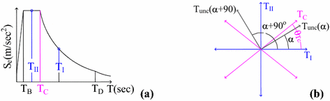

  

  Position of T_I and T_II on the response spectrum (a) and relative position of the two orthogonal T_unc (b)

In this case, T_unc(α) falls on different branches of the spectrum depending on the angle α. As a result, S_e is expressed by different equations as a function of α and F(α) has multiple branches, where at least one of these branches is a function of α. The base shear of the perpendicular direction F(α + 90°) is expressed following the same rules. The relative position of T_unc(α) and T_unc(α + 90°) for a given angle α, shown in Fig. 10b, affects the development of Eqs. (15), (28) and (30). It can be seen in Fig. 10b that the angle θ_Tc corresponding to the corner period T_C determines the angle range of the branches of the final expression. To illustrate the formulation of Eqs. (15), (28) and (30), the relative position of T_unc(α) and T_unc(α + 90°) is presented in Fig. 11 for all ASIs and for all three cases with respect to the angle θ_Tc. The solid hatched areas represent the position of T_unc(α), while the dashed hatched areas represent the respective position of T_unc(α + 90°). As a result, Eqs. (15), (28) and (30) comprise eight branches with specific angle range limits. The terms F(α) and F(α + 90°) of Eq. (15) that are used to form the piecewise equation are presented in Eq. (40) for the first case of Fig. 11, i.e. θ_Tc < 45° and ω = 0.

Fig. 11

Determination of the branches of the piecewise equation

$$\left\{ {\begin{array}{*{20}l} {\begin{array}{*{20}c} { 2 {{\uppi }} -\uptheta_{{{\text{T}}_{\text{c}} }} \le {{\upalpha }} \le\uptheta_{{{\text{T}}_{\text{c}} }} } \\ {\text{and}} \\ {\uptheta_{{{\text{T}}_{\text{c}} }} \le {{\upalpha \,+\, 90}}^{ \circ } \le {{\uppi }} -\uptheta_{{{\text{T}}_{\text{c}} }} } \\ \end{array} } \hfill & \Rightarrow \hfill & {{\text{F}}(\upalpha ) = \frac{{{\text{T}}_{\text{C}} \cdot {\text{a}}_{\text{g}} \cdot {\text{S}} \cdot {{\upeta }} \cdot 2. 5}}{{\frac{{{\text{T}}_{\text{I}} \cdot {\text{T}}_{\text{II}} }}{{\sqrt {{ \cos }\left( {{\upalpha }} \right)^{ 2} \cdot {\text{T}}_{\text{II}}^{ 2} {\text{ + sin}}\left( {{\upalpha }} \right)^{ 2} \cdot {\text{T}}_{\text{I}}^{ 2} } }}}},} \hfill & {{\text{F}}(\upalpha + 9 0^{ \circ } )= {\text{a}}_{\text{g}} \cdot {\text{S}} \cdot {{\upeta }} \cdot 2. 5} \hfill \\ {\begin{array}{*{20}c} {\uptheta_{{{\text{T}}_{\text{c}} }} \, \le \,\,{{\upalpha }}\, \le \,{{\uppi }}\,{ - }\,\uptheta_{{{\text{T}}_{\text{c}} }} } \\ {\text{and}} \\ {\uptheta_{{{\text{T}}_{\text{c}} }} \le {{\upalpha \,+\, 90}}^{ \circ } \le {{\uppi }} -\uptheta_{{{\text{T}}_{\text{c}} }} } \\ \end{array} } \hfill & \Rightarrow \hfill & {{\text{F}}(\upalpha ) = {\text{a}}_{\text{g}} \cdot {\text{S}} \cdot {{\upeta }} \cdot 2. 5,} \hfill & {{\text{F}}(\upalpha + 9 0^{ \circ } )= {\text{a}}_{\text{g}} \cdot {\text{S}} \cdot {{\upeta }} \cdot 2. 5} \hfill \\ {\begin{array}{*{20}c} {\uptheta_{{{\text{T}}_{\text{c}} }} \, \le \,\,{{\upalpha }}\, \le \,{{\uppi }}\,{ - }\,\uptheta_{{{\text{T}}_{\text{c}} }} } \\ {\text{and}} \\ {{{\uppi }}\,{ - }\,\uptheta_{{{\text{T}}_{\text{c}} }} \, \le \,{{\upalpha }}\,{ + }\, 9 0^{ \circ } \, \le \,{{\uppi }}\,{ + }\,\uptheta_{{{\text{T}}_{\text{c}} }} } \\ \end{array} } \hfill & \Rightarrow \hfill & {{\text{F}}(\upalpha ) = {\text{a}}_{\text{g}} \cdot {\text{S}} \cdot {{\upeta }} \cdot 2. 5,} \hfill & {{\text{F}}(\upalpha \,+\, 90^{ \circ } )= \frac{{{\text{T}}_{\text{C}} \cdot {\text{a}}_{\text{g}} \cdot {\text{S}} \cdot {{\upeta }} \cdot 2. 5}}{{\frac{{{\text{T}}_{\text{I}} \cdot {\text{T}}_{\text{II}} }}{{\sqrt {{ \cos }\left( {{{\upalpha \,+\, 90}}^{ \circ } } \right)^{ 2} \cdot {\text{T}}_{\text{II}}^{ 2} + { \sin }\left( {{{\upalpha \,+\, 90}}^{ \circ } } \right)^{ 2} \cdot {\text{T}}_{\text{I}}^{ 2} } }}}}} \hfill \\ {\begin{array}{*{20}c} {\theta_{{T_{c} }} \, \le \,\alpha \, \le \,\pi \, - \,\theta_{{T_{c} }} } \\ {\text{and}} \\ {\pi \, + \,\theta_{{T_{c} }} \, \le \,\,\alpha \, + \,90^{ \circ } \, \le \,2\,\pi \, - \,\theta_{{T_{c} }} } \\ \end{array} } \hfill & \Rightarrow \hfill & {{\text{F}}(\upalpha ) = {\text{a}}_{\text{g}} \cdot {\text{S}} \cdot {{\upeta }} \cdot 2. 5,} \hfill & {{\text{F}}(\upalpha \,+\, 90^{ \circ } )= {\text{a}}_{\text{g}} \cdot {\text{S}} \cdot {{\upeta }} \cdot 2. 5} \hfill \\ {\begin{array}{*{20}c} {{{\uppi }}\,{ - }\,\uptheta_{{{\text{T}}_{\text{c}} }} \, \le \,\,{{\upalpha }}\, \le \,{{\uppi }}\,{ + }\,\uptheta_{{{\text{T}}_{\text{c}} }} } \\ {\text{and}} \\ {{{\uppi }}\,{ + }\,\uptheta_{{{\text{T}}_{\text{c}} }} \, \le \,\,{{\upalpha }}\,{ + }\, 9 0^{ \circ } \, \le \, 2 {{\uppi }}\,{ - }\,\uptheta_{{{\text{T}}_{\text{c}} }} } \\ \end{array} } \hfill & \Rightarrow \hfill & {{\text{F}}(\upalpha ) = \frac{{{\text{T}}_{\text{C}} \cdot {\text{a}}_{\text{g}} \cdot {\text{S}} \cdot {{\upeta }} \cdot 2. 5}}{{\frac{{{\text{T}}_{\text{I}} \cdot {\text{T}}_{\text{II}} }}{{\sqrt {{ \cos }\left( {{\upalpha }} \right)^{ 2} \cdot {\text{T}}_{\text{II}}^{ 2} {\text{ + sin}}\left( {{\upalpha }} \right)^{ 2} \cdot {\text{T}}_{\text{I}}^{ 2} } }}}},} \hfill & {{\text{F}}(\upalpha \,+\, 90^{ \circ } )= {\text{a}}_{\text{g}} \cdot {\text{S}} \cdot {{\upeta }} \cdot 2. 5} \hfill \\ {\begin{array}{*{20}c} {{{\uppi }}\,{ + }\,\uptheta_{{{\text{T}}_{\text{c}} }} \, \le \,\,{{\upalpha }}\, \le \, 2 {{\uppi }}\,{ - }\,\uptheta_{{{\text{T}}_{\text{c}} }} } \\ {\text{and}} \\ {{{\uppi }}\,{ + }\,\uptheta_{{{\text{T}}_{\text{c}} }} \, \le \,\,{{\upalpha }}\,{ + }\, 9 0^{ \circ } \, \le \, 2 {{\uppi }}\,{ - }\,\uptheta_{{{\text{T}}_{\text{c}} }} } \\ \end{array} } \hfill & \Rightarrow \hfill & {{\text{F}}(\upalpha ) = {\text{a}}_{\text{g}} \cdot {\text{S}} \cdot {{\upeta }} \cdot 2. 5,} \hfill & {{\text{F}}(\upalpha \,+\, 90^{ \circ } )= {\text{a}}_{\text{g}} \cdot {\text{S}} \cdot {{\upeta }} \cdot 2. 5} \hfill \\ {\begin{array}{*{20}c} {{{\uppi }}\,{ + }\,\uptheta_{{{\text{T}}_{\text{c}} }} \, \le \,\,{{\upalpha }}\, \le \, 2 {{\uppi }}\,{ - }\,\uptheta_{{{\text{T}}_{\text{c}} }} } \\ {\text{and}} \\ { 2 {{\uppi }}\,{ - }\,\uptheta_{{{\text{T}}_{\text{c}} }} \, \le \,\,{{\upalpha }}\,{ + }\, 9 0^{ \circ } \, \le \,\uptheta_{{{\text{T}}_{\text{c}} }} } \\ \end{array} } \hfill & \Rightarrow \hfill & {{\text{F}}(\upalpha ) = {\text{a}}_{\text{g}} \cdot {\text{S}} \cdot {{\upeta }} \cdot 2. 5,} \hfill & {{\text{F}}(\upalpha \,+\, 90^{ \circ } )= \frac{{{\text{T}}_{\text{C}} \cdot {\text{a}}_{\text{g}} \cdot {\text{S}} \cdot {{\upeta }} \cdot 2. 5}}{{\frac{{{\text{T}}_{\text{I}} \cdot {\text{T}}_{\text{II}} }}{{\sqrt {{ \cos }\left( {{{\upalpha \,+\, 90}}^{ \circ } } \right)^{ 2} \cdot {\text{T}}_{\text{II}}^{ 2} + { \sin }\left( {{{\upalpha \,+\, 90}}^{ \circ } } \right)^{ 2} \cdot {\text{T}}_{\text{I}}^{ 2} } }}}}} \hfill \\ {\begin{array}{*{20}c} {{{\uppi }}\,{ + }\,\uptheta_{{{\text{T}}_{\text{c}} }} \, \le \,\,{{\upalpha }}\, \le \, 2 {{\uppi }}\,{ - }\,\uptheta_{{{\text{T}}_{\text{c}} }} } \\ {\text{and}} \\ {\uptheta_{{{\text{T}}_{\text{c}} }} \, \le \,\,{{\upalpha }}\,{ + }\, 9 0^{ \circ } \, \le \,{{\uppi }}\,{ - }\,\uptheta_{{{\text{T}}_{\text{c}} }} } \\ \end{array} } \hfill & \Rightarrow \hfill & {{\text{F}}(\upalpha ) = {\text{a}}_{\text{g}} \cdot {\text{S}} \cdot {{\upeta }} \cdot 2. 5,} \hfill & {{\text{F}}(\upalpha \,+\, 90^{ \circ } )= {\text{a}}_{\text{g}} \cdot {\text{S}} \cdot {{\upeta }} \cdot 2. 5} \hfill \\ \end{array} } \right.$$

(40)

References

Anastassiadis K, Avramidis I, Panetsos P (2002) Concurrent design forces in structures under three-component orthotropic seismic excitation. Earthq Spectra 18(1):1–17
Anastassiadis K (1985) Caracteristiques elastiques spatiales des batiments a etages. Annales de l’ITBTP (No. 435)
Anastassiadis K (1989) Antiseismic structures, vol I. ZITI, Thessaloniki
ASCE (2014) Seismic evaluation and retrofit of existing buildings (ASCE/SEI 41-13). American Society of Civil Engineers, Reston
Athanatopoulou AM (2005) Critical orientation of three correlated seismic components. Eng Struct 27(2):301–312
Athanatopoulou AM, Doudoumis IN (2008) Principal directions under lateral loading in multistorey asymmetric buildings. Struct Des Tall Spec Build 17(4):773–794
Athanatopoulou AM, Makarios T, Anastassiadis K (2006) Earthquake analysis of isotropic asymmetric multistorey buildings. Struct Des Tall Spec Build 15(4):417–443
Cantagallo C, Camata G, Spacone E (2015) Influence of ground motion selection methods on seismic directionality effects. Earthq Struct 8(1):185–204
CEN (2004) EN1998-1 Eurocode 8: design of structures for earthquake resistance, part 1: general rules, seismic actions and rules for buildings. European Committee for Standarization, Brussels
CEN (2005) EN1998-3 Eurocode 8: design of structures for earthquake resistance, part 3: assessment and retrofitting of buildings. European Committee for Standarization, Brussels
Doudoumis IN, Athanatopoulou AM (2008) Invariant torsion properties of multistorey asymmetric buildings. Struct Des Tall Spec Build 17(1):79–97
EAK (2003) Greek code for earthquake resistant design of structures. Ministry of Environment, Planning and Public Works, Athens
Federal Emergency Management Agency (2012) Seismic performance assessment of buildings. FEMA P58 report, Washington, DC
Fontara IK, Konstantinos M, Kostinakis G, Manoukas G, Athanatopoulou AM (2015) Parameters affecting the seismic response of buildings under bi-directional excitation. Struct Eng Mech 53(5):957–979
Guyan RJ (1965) Reduction of stiffness and mass matrices. AIAA J 3(2):380
Kostinakis KG, Athanatopoulou AM, Avramidis IE (2013a) Evaluation of inelastic response of 3D single-story R/C frames under bi-directional excitation using different orientation schemes. Bull Earthq Eng 11(2):637–661
Kostinakis KG, Athanatopoulou AM, Tsiggelis VS (2013b) Effectiveness of percentage combination rules for maximum response calculation within the context of linear time history analysis. Eng Struct 56:36–45
Lagaros ND (2010) Multicomponent incremental dynamic analysis considering variable incident angle. Struct Infrastruct Eng 6(1–2):77–94
Lopez OA, Chopra AK, Hernandez JJ (2001) Evaluation of combination rules for maximum response calculation in multicomponent seismic analysis. Earthq Eng Struct Dyn 30(9):1379–1398
MacRae AG, Mattheis J (2000) Three-dimentional steel building response to near-fault motions. J Struct Eng ASCE 126(1):117–126
Magliulo G, Maddaloni G, Petrone C (2014) Influence of earthquake direction on the seismic response of irregular plan RC frame buildings. Earthq Eng Eng Vib 13(2):243–256
Makarios TK, Anastassiadis K (1998) Real and fictitious elastic axes of multi-storey buildings: theory. Struct Des Tall Spec Build 7(1):33–55
Maple 18 (2002) Maplesoft, a Division of Waterloo Maple Inc. Waterloo, Ontario
Marino EM, Rossi PP (2004) Exact evaluation of the location of the optimum torsion axis. Struct Des Tall Spec Build 13(4):277–290
McKenna F, Fenves GL, Jeremic B, Scott MH (2000) Open system for earthquake engineering simulation. http://opensees.berkeley.edu/
Menun C, Der Kiureghian A (1998) A Replacement for the 30%, 40%, and SRSS rules for multicomponent seismic analysis. Earthq Spectra 14(1):153–163
Morfidis KE, Athanatopoulou AM, Avramidis IE (2008) Effects of seismic directivity within the framework of the lateral force procedure. In: 14th World conference on earthquake engineering. Beijing, China
Newmark N (1975) Seismic design criteria for structures and facilities: trans-Alaska pipeline system. In: U.S. National conference in earthquake engineering. Ann Arbor, Michigan
NTC (2008) Norme tecniche per le costruzioni. Decreto del Ministero delle Infrastrutture. Supplemento ordinario n.30 alla Gazzetta Ufficiale della Repubblica Italiana n.29 del 4/02/2008, Italy (in Italian)
Palermo M, Silvestri S, Gasparini G, Trombetti T (2013) Physically-based prediction of the maximum corner displacement magnification of one-storey eccentric systems. Bull Earthq Eng 11(5):1467–1491
Penzien J, Watabe M (1975) 3-Dimensional earthquake ground motions. Earthq Eng Struct Dyn 3(4):365–373
Regulatory Guide 1.92 (2006) U.S. Nuclear Regulatory Commission, Office of Nuclear Regulatory Research. Washington, DC
Riddel R, Vasquez J (1984) Existence of centers of resistance and torsional uncoupling of earthquake response of buildings. In: 8th World conference on earthquake engineering. San Francisco, USA, pp 187–194
Rigato AB, Medina RA (2007) Influence of angle of incidence on seismic demands for inelastic single-storey structures subjected to bi-directional ground motions. Eng Struct 29(10):2593–2601
Rosenblueth E, Contreras H (1977) Approximate design for multi-component earthquakes. J Eng Mech Div 103(5):881–893
Roussopoulos A (1932) Distribution of horizontal forces by a rigid plate in spatial structures: case of seismic forces, their distribution and regime. Tech Chron Tech Chamb Greece 17:871–884 (In Greek)
Toranzo-Diandera LA (2009) Evaluation of the ASCE 41 linear elastic procedure for seismic retrofit of existing structures: pros and cons of the method. In: ATC & SEI 2009 conference on improving the seismic performance of existing buildings and other structures. San Francisco, California, pp 85–91
Wilson EL, Suharwardy I, Habibullah A (1995) A clarification of the orthogonal effects in a three-dimensional seismic analysis. Earthq Spectra 11(4):659–666
Acknowledgements
Financial support of the Portuguese Foundation for Science and Technology, through the Ph.D. Grant of the first author (PD/BD/113681/2015), is gratefully acknowledged.
Author information
Authors and Affiliations
Corresponding author