A Categorical Construction for the Computational Definition of Vector Spaces

Abstract

Lambda-${\mathcal {S}}$ is an extension to first-order lambda calculus unifying two approaches of non-cloning in quantum lambda-calculi. One is to forbid duplication of variables, while the other is to consider all lambda-terms as algebraic linear functions. The type system of Lambda-${\mathcal {S}}$ has a constructor S such that a type A is considered as the base of a vector space while S(A) is its span. Lambda-${\mathcal {S}}$ can also be seen as a language for the computational manipulation of vector spaces: The vector spaces axioms are given as a rewrite system, describing the computational steps to be performed. In this paper we give an abstract categorical semantics of Lambda-${\mathcal {S}}^{*}$ (a fragment of Lambda-${\mathcal {S}}$), showing that S can be interpreted as the composition of two functors in an adjunction relation between a Cartesian category and an additive symmetric monoidal category. The right adjoint is a forgetful functor U, which is hidden in the language, and plays a central role in the computational reasoning.

A Detailed Proofs

Proposition 4.9

(Independence of derivation) If $\varGamma \vdash t:A$ can be derived with two different derivations $\pi$ and $\pi '$, then $\llbracket {\pi }\rrbracket =\llbracket {\pi '}\rrbracket$

Proof

Without taking into account rules $\Rightarrow _E$, $\Rightarrow _{SE}$ and $S_I$, the typing system is syntax directed. In the case of the application (rules $\Rightarrow _E$ and $\Rightarrow _{SE}$), they can be interchanged only in few specific cases.

Hence, we give a rewrite system on trees such that each time a rule $S_I$ can be applied before or after another rule, we chose a direction to rewrite the three to one of these forms. Similarly we chose a direction for rules $\Rightarrow _E$ and $\Rightarrow _{ES}$. Then we prove that every rule preserves the semantics of the tree. This rewrite system is clearly confluent and normalizing, hence for each tree $\pi$ we can take the semantics of its normal form, and so every sequent will have one way to calculate its semantics: as the semantics of the normal tree.

In order to define the rewrite system, we first analyze the typing rules containing only one premise, and check whether these rules allow for a previous and posterior rule $S_I$. If both are allowed, we choose a direction for the rewrite rule. Then we continue with rules with more than one premise and check under which conditions a commutation of rules is possible, choosing also a direction.

Rules with one premise:

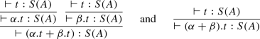
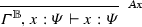
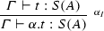
• Rule $\alpha _I$:

  

  (A.1)

• Rules $\Rightarrow _I$, $\times _{E_r}$, $\times _{E_l}$, $\Uparrow _r$, and $\Uparrow _\ell$: These rules end with a specific types not admitting two S in the head position (i.e. ${\mathbb {B}}^j\times S({\mathbb {B}}^{n-j})$, $\varPsi \Rightarrow A$, ${\mathbb {B}}$, ${\mathbb {B}}^{n-1}$, and $S(\varPsi \times \varPhi )$) hence removing an S or adding an S would not allow the rule to be applied, and hence, these rules followed or preceded by $S_I$ cannot commute.

Rules with more than one premise:

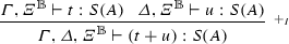
• Rule $+_I$:

  

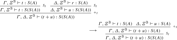  (A.2)

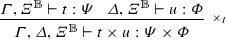
• Rules $\Rightarrow _E$ and $\Rightarrow _{ES}$:

  

  (A.3)

• Rules If and $\times _I$: These rules end with a specific types not admitting two S in the head position (i.e. ${\mathbb {B}}\Rightarrow A$ and $\varPsi \times \varPhi$), hence removing an S or adding an S would not allow the rule to be applied, and hence, these rules followed or preceded by $S_I$ cannot commute.

The confluence of this rewrite system is easily inferred from the fact that there are not critical pairs. The strong normalization follows from the fact that the trees are finite and all the rewrite rules push the $S_I$ to the root of the trees.

It only remains to check that each rule preserves the semantics.

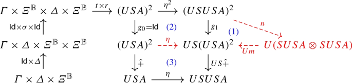
• Rule (A.1): The following diagram gives the semantics of both trees (we only treat, without lost of generality, the case where $A\ne S(A')$).

  

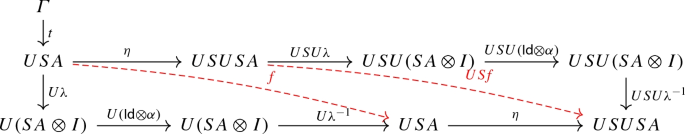
  Let $h = \lambda ^{-1}\circ (\mathsf {Id}\otimes \alpha )\circ \lambda$ and $f=Uh$. The diagram commutes by naturality of $\eta$ with respect to f.

• Rule (A.2): The following diagram gives the semantics of both trees (we only treat, without lost of generality, the case where $A\ne S(A')$).

  

  • 1. Definition of $g_1$.

  • 2. $\eta$ is a monoidal natural transformation.

  • 3. Naturality of $\eta$ with respect to $\hat{+}$.

• Rule (A.3): The following diagram gives the semantics of both trees.

• 1. Naturality of $\eta$ with respect to $\varepsilon ^\varPsi$.

• 2. $\eta$ is a monoidal natural transformation.

$\square$

Lemma A.1

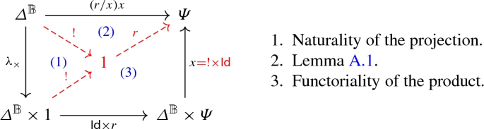
(Weakening) If $\varGamma \vdash t:A$, then $\varGamma ,\varDelta ^{\mathbb {B}}\vdash t:A$. Moreover, $\llbracket {\varGamma ,\varDelta ^{\mathbb {B}}\vdash t:A}\rrbracket =\llbracket {\varGamma \vdash t:A}\rrbracket \circ (\mathsf {Id}\times {!})$.

Proof

It is easy to show that a tree deriving $\varGamma \vdash t:A$ can be transformed into a tree deriving $\varGamma ,\varDelta ^{\mathbb {B}}\vdash t:A$ just by adding $\varDelta ^{\mathbb {B}}$ to the contexts in its axioms. Moreover, since $FV(t)\cap \varDelta ^{\mathbb {B}}=\emptyset$, we have $\llbracket {\varGamma ,\varDelta ^{\mathbb {B}}\vdash t:A}\rrbracket =\llbracket {\varGamma \vdash t:A}\rrbracket \circ (\mathsf {Id}\times {!})$. $\square$

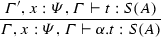
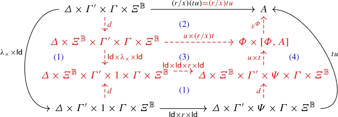
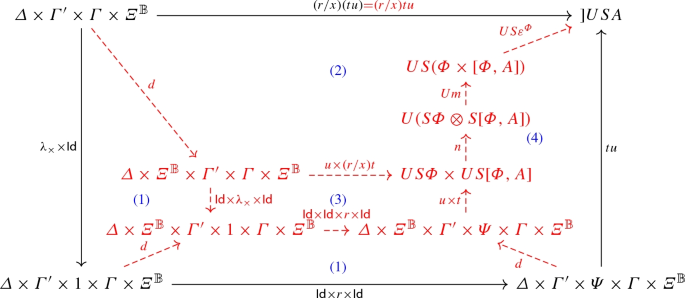
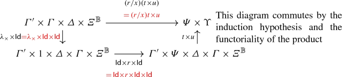
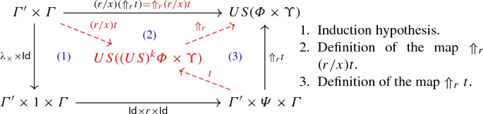
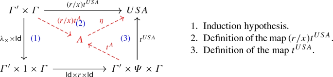
Lemma 4.10

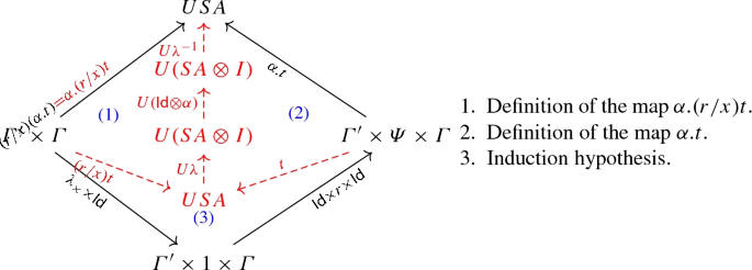
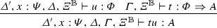
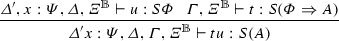
(Substitution) If $\varGamma ',x:\varPsi ,\varGamma \vdash t:A$ and $\vdash r:\varPsi$, then the following diagram commutes:

That is, $\llbracket {\varGamma '\times \varGamma \vdash (r/x)t:A}\rrbracket =\llbracket {\varGamma ,x:\varPsi ,\varGamma '\vdash t:A}\rrbracket \circ (\mathsf {Id}\times \llbracket {\vdash r:\varPsi }\rrbracket \times \mathsf {Id})$.

Proof

By induction on the derivation of $\varGamma ',x:\varPsi ,\varGamma \vdash t:A$. Also, we take the rules $\alpha _I$ and $+_I$ with $m=1$, the generalization is straightforward.

• 

  

• 

  

•    We only treat the case when $x\in FV(t)$, the cases $x\in FV(u)$ and $x\in FV(u)\cap FV(t)$ are analogous.

  

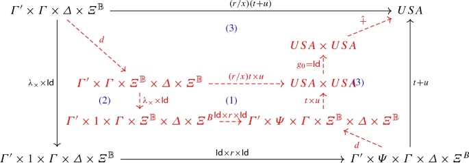
  • 1. Induction hypothesis.

  • 2. Naturality of d.

  • 3. Definition of $+$.

• 

  

• 

  

• 

  

  • 1. Naturality of d.

  • 2. Definition of the map (r/x)tu.

  • 3. Induction hypothesis and functoriality of the product.

  • 4. Definition of the map tu.

•       Analogous to previous case.

• 

  

  • 1. Naturality of d.

  • 2. Definition of the map (r/x)tu.

  • 3. Induction hypothesis and functoriality of the product.

  • 4. Definition of the map tu.

•       Analogous to previous case.

• 

  

•       Analogous to previous case.

• 

  

• 

  

• 

  

•       Analogous to previous case.

• 

  

$\square$

Theorem 4.11

(Soundness) If $\vdash t:A$, and $t\longrightarrow r$, then $\llbracket {\vdash t:A}\rrbracket = \llbracket {\vdash r:A}\rrbracket$.

Proof

By induction on the rewrite relation, using the first derivable type for each term. We take the rules $\alpha _I$ and $+_I$ with $m=1$, the generalization is straightforward.

$(\mathsf {comm})$:

$(t+r)=(r+t)$. We have

Then,

Where $\gamma$ is the symmetry on $\times$ and $\sigma$ the symmetry on $\oplus$.

$(\mathsf {asso})$:

$((t+r)+s)=(t+(r+s))$. We have

Then

• 1. Naturality of $\alpha _\times$.

• 2. Definition of $\hat{+}$.

• 3. U monoidal functor.

• 4. Naturality of p with respect to $\nabla$.

• 5. Associativity property of $\oplus$.

($\beta _b$):

If b has type ${\mathbb {B}}^n$ and $b\in \mathsf B$, then $(\lambda x{:}{{\mathbb {B}}^n}.t)b\longrightarrow (b/x)t$. We have,

Then,

This diagram commutes because of Lemma 4.10.

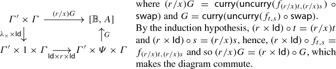
($\beta _n$):

If u has type $S\varPsi$, then $(\lambda x{:}{S\varPsi }.t)u\longrightarrow (u/x)t$. We have,

Then,

This diagram commutes because of Lemma 4.10.

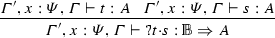
($\mathsf {If}_1$):

${|1\rangle }?{t}\mathord {\cdot }{r}\longrightarrow t$. We have,

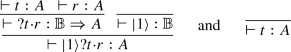
Then,

Notice that $\mathsf {curry}(\mathsf {uncurry}(f_{t,r})\circ \mathsf {swap})$ transforms the arrow ${\mathbb {B}}\xrightarrow {f_{t,r}}[1,A]$ (which is the arrow $|0\rangle \mapsto r$, $|1\rangle \mapsto t$) into an arrow ${1}\xrightarrow {}[{\mathbb {B}},A]$, and hence, $\varepsilon \circ (i_2\times \mathsf {curry}(\mathsf {uncurry}(f_{t,r})\circ \mathsf {swap}))=t$.

($\mathsf {If}_0$):

Analogous to ($\mathsf {If}_1$).

($\mathsf {lin}_r^+$):

If t has type ${\mathbb {B}}^n\Rightarrow A$, then $t(u+v)\longrightarrow tu+tv$. We have,

and

• 1. Definition of $\hat{+}$.

• 2. Naturality of $\nabla$.

• 3. Axiom$_{{}_{\mathsf {Dist}}}$.

• 4. Let $f=\pi _1\otimes \mathsf {Id}$, $g=\pi _2\otimes \mathsf {Id}$, and $A=B=S{\mathbb {B}}^n\otimes [{\mathbb {B}}^n,A]$. Hence,

  $$\begin{aligned} \nabla \circ \delta= & {} [\mathsf {Id},\mathsf {Id}]\circ \langle f,g\rangle \\= & {} [\mathsf {Id},\mathsf {Id}]\circ \mathsf {Id}\circ \langle f,g \rangle \\= & {} [\mathsf {Id},\mathsf {Id}]\circ (i_A\circ \pi _A+i_B\circ \pi _B)\circ \langle f,g \rangle \\= & {} (([\mathsf {Id},\mathsf {Id}]\circ i_A\circ \pi _A)+([\mathsf {Id},\mathsf {Id}]\circ i_B\circ \pi _B))\circ \langle f,g \rangle \\= & {} (\pi _A+\pi _B)\circ \langle f,g \rangle \\= & {} \pi _A\circ \langle f,g \rangle +\pi _B\circ \langle f,g \rangle \\= & {} f+g\\= & {} \pi _1\otimes \mathsf {Id}+\pi _2\otimes \mathsf {Id}\\= & {} \nabla \otimes \mathsf {Id}\end{aligned}$$

• 5. Naturality of $\hat{+}$.

• 6. Naturality of $\varDelta$.

• 7. Definition of d.

• 8. Naturality of $\sigma$.

$(\mathsf {lin}_r^ \alpha )$:

If t has type ${\mathbb {B}}^n\Rightarrow A$, then $t(\alpha .u)\longrightarrow \alpha .(tu)$. We have,

Then,

• 1. Functoriality of $\times$.

• 2. Naturality of n.

• 3. Coherence of $\sigma$.

• 4. Naturality of $\lambda$ with respect to m.

• 5. Functoriality of $\otimes$.

• 6. Naturality of $\lambda$ with respect to $S\varepsilon ^{{\mathbb {B}}^n}$.

• 7. Naturality of $\lambda ^{-1}$ with respect to m.

$(\mathsf {lin}^0_r)$:

If t has type ${\mathbb {B}}^n\Rightarrow A$, then $t\mathbf {0}_{S({\mathbb {B}}^n)}\longrightarrow \mathbf {0}_{S(A)}$. We have,

Then,

• 1. Naturality of $\eta$ and functoriality of the product.

• 2. Naturality of n.

• 3. Property of monoidal adjunctions.

• 4. Notice that $\mathbf 0\otimes (St\circ m_I)=\mathbf 0$, hence, this diagram commutes by property of $\mathbf 0$.

• 5. Property of the morphism $\mathbf 0$.

• 6. Property of monoidal categories.

• 7. Naturality of $\lambda _\times$.

$(\mathsf {lin}^+_l)$:

$(t+u)v\longrightarrow (tv+uv)$. This case is analogous to $(\mathsf {lin}^+_r)$. Notice that the axiom is valid only for $\hat{+}\times \mathsf {Id}$, not for $\mathsf {Id}\times \hat{+}$, however, one can be transformed into the other by using a swap.

$(\mathsf {lin}^\alpha _l)$:

$(\alpha .t)u\longrightarrow \alpha .(tu)$. This case is analogous to $(\mathsf {lin}^\alpha _r)$.

$(\mathsf {lin}^0_l)$:

$\mathbf {0}_{S({\mathbb {B}}^n\Rightarrow A)}t\longrightarrow \mathbf {0}_{S(A)}$. This case is analogous to $(\mathsf {lin}^0_r)$.

$(\mathsf {neutral})$:

$(\mathbf {0}_{S(A)}+t)\longrightarrow t$. We have

Then,

• 1. By Axiom$_{{}_0}$ and functoriality of product.

• 2. Naturality of p.

• 3. Definition of $\hat{+}$.

• 4. Naturality of $\varDelta$.

• 5. U preserves product.

• 6. Property of sum in an additive category.

• 7. The map $\mathbf 0$ is neutral with respect to the sum.

$(\mathsf {unit})$:

$1.t\longrightarrow t$. We have

Then,

$(\mathsf {zero}_\alpha )$:

If t has type A, $0.t\longrightarrow \mathbf {0}_{S(A)}$. We have

Then,

• 1. Axiom$_{{}_0}$.

• 2. Property of the map $\mathbf 0$.

$(\mathsf {zero})$:

$\alpha .\mathbf {0}_{S(A)}\longrightarrow \mathbf {0}_{S(A)}$. We have

Then

• 1. Same arrows.

• 2. Property of the morphism $\mathbf 0$.

$(\mathsf {prod})$:

$\alpha .(\beta .t)\longrightarrow (\alpha \beta ).t$. We have

Then

This diagram commutes by functoriality of $\otimes$.

$(\alpha \mathsf {dist})$:

$\alpha .(t+u)\longrightarrow \alpha .t+\alpha .u$. We have

Then

The three subdiagrams are valid by the naturality of $\hat{+}$.

$(\mathsf {fact})$:

$(\alpha .t+\beta .t)\longrightarrow (\alpha +\beta ).t$. We have

Then

• 1. Naturality of $\varDelta$.

• 2. Functor U preserves product.

• 3. Distributivity property given by the fact that the tensor is a left adjoint.

• 4. Naturality of $p^{-1}$.

• 5. Additivity of the category.

• 6. Definition of $\hat{+}$.

• 7. Naturality of $\hat{+}$.

$(\mathsf {fact}^1)$:

$(\alpha .t+t)\longrightarrow (\alpha +1).t$. This case is a particular case of $\mathsf {fact}$.

$(\mathsf {fact}^2)$:

$(t+t)\longrightarrow 2.t$. This case is a particular case of $\mathsf {fact}$.

$(\mathsf {head})$:

If $h\ne u\times v$, and $h\in \mathsf B$, $\text { head}\ h\times t\longrightarrow h$. We have

Then

This diagram commutes since $\pi _1$ is just the projection.

$(\mathsf {tail})$:

If $h\ne u\times v$, and $h\in \mathsf B$, $\text { tail}\ h\times t\longrightarrow t$. We have

Then

This diagram commutes since $\pi _2$ is just the projection.

($\mathsf {dist}_r^+$):

$\Uparrow _r ((r+s)\times u)\longrightarrow \Uparrow _r (r\times u)+\Uparrow _r (s\times u)$. We have,

Then

• 1. Functoriality of the product.

• 2. Naturality of $\eta$.

• 3. Naturality of $\eta$ (remark that by the axioms of monads, $\mu \circ \eta =\mathsf {Id}$).

• 4. Naturality of d.

• 5. Axiom$_{{}_{\mathsf {Dist}}}$ and definition of $\hat{+}$.

• 6. Naturality of $\hat{+}$.

($\mathsf {dist}_l^+$):

$\Uparrow _\ell u\times (r+s)\longrightarrow \Uparrow _\ell (u\times r)+\Uparrow _\ell (u\times s)$. Analogous to case $(\mathsf {dist}_r^+)$

$({{\mathsf {dist}}^{\alpha }_{\mathsf {r}}})$:

$\Uparrow _r (\alpha .r)\times u\longrightarrow \alpha .\Uparrow _r r\times u$. We have,

Then

• 1. See next diagram.

• 2. Naturality of $\eta$.

• 3. Functoriality of product.

• 4. Naturality of n.

• 5. Coherence.

• 6. Naturality of $\lambda$.

• 1. Naturality of $\eta$.

• 2. Functoriality of the product.

• 3. Naturality of n.

• 4. Coherence

• 5. Naturality of $\lambda$ and functoriality of USU.

• 6. Naturality of $\sigma$.

• 7. Functoriality of the tensor.

$({{\mathsf {dist}}^{\alpha }_{\mathsf {l}}})$:

$\Uparrow _\ell u\times (\alpha .r)\longrightarrow \alpha .\Uparrow _\ell u\times r$. Analogous to case $({{\mathsf {dist}}^{\alpha }_{\mathsf {r}}})$.

$(\mathsf {dist}^0_{\mathsf {r}})$:

If u has type $\varPhi$, $\Uparrow _r\mathbf {0}_{S(\varPsi )}\times u\longrightarrow \mathbf {0}_{S(\varPsi \times \varPhi )}$. We have

Then

• 1. Naturality of $\eta$.

• 2. Functoriality of the product.

• 3. Naturality of $\varDelta$.

• 4. $U(\mathbf{0}\otimes Su)=U\mathbf{0}$, hence, we conclude by Axiom$_{{}_0}$ with the maps $n\circ \varDelta$ and $\mathsf {Id}$.

• 5. Naturality of n.

• 6. Property of map $\mathbf{0}$.

$(\mathsf {dist}^0_{\mathsf {l}})$:

If u has type $\varPsi$, $\Uparrow _\ell u\times \mathbf {0}_{S(\varPhi )}\longrightarrow \mathbf {0}_{S(\varPsi \times \varPhi )}$. Analogous to case $(\mathsf {dist}^0_{\mathsf {r}})$.

($\mathsf {dist}_\Uparrow ^+$):

$\Uparrow (t+u)\longrightarrow (\Uparrow t+\Uparrow u)$. We only give the details for $\Uparrow _r$, the case $\Uparrow _\ell$ is analogous.

Then

This diagram commutes by naturality of $\hat{+}$.

($\mathsf {dist}_\Uparrow ^\alpha$):

$\Uparrow (\alpha .t)\longrightarrow \alpha .\Uparrow t$. We only give the details for $\Uparrow _r$, the case $\Uparrow _\ell$ is similar.

Then

• 1. Naturality of $\lambda$.

• 2. Naturality of $\lambda$ and the definition of monad given by an adjunction.

• 3. Functoriality of tensor.

• 4. Naturality of $\lambda ^{-1}$.

• 5. Naturality of $\lambda ^{-1}$ and the definition of monad given by an adjunction.

$({\mathsf {dist}}^{\mathsf {0}}_{\Uparrow _{\mathsf {r}}})$:

$\Uparrow _r\mathbf {0}_{S(S(S\varPsi )\times \varPhi )}\longrightarrow \Uparrow _r\mathbf {0}_{S(S\varPsi \times \varPhi )}$. We have

Then,

This diagram commutes by the property of the map $\mathbf{0}$.

$({\mathsf {dist}}^{\mathsf {0}}_{\Uparrow _\ell })$:

$\Uparrow _\ell \mathbf {0}_{S(\varPhi \times S(S\varPsi ))}\longrightarrow \Uparrow _\ell \mathbf {0}_{S(\varPhi \times S\varPsi )}$. Analogous to case $({\mathsf {dist}}^{\mathsf {0}}_{\Uparrow _{\mathsf {r}}})$.

$({\mathsf {neut}}^\Uparrow _{\mathsf {r}})$:

If $u\in \mathsf B$, $\Uparrow _r u\times v\longrightarrow u\times v$. We have

Then

• 1. Naturality of $\eta$.

• 2. Functoriality of product.

• 3. Remark that $\mu \circ US\eta = \mathsf {Id}$.

• 4. $\eta$ is a monoidal linear transformation.

$({\mathsf {neut}}^{\Uparrow }_{\ell })$:

If $v\in \mathsf B$, $\Uparrow _\ell u\times v\longrightarrow u\times v$. Analogous to case $({\mathsf {neut}}^\Uparrow _{\mathsf {r}})$.

$({\mathsf {neut}}^\Uparrow _{\mathsf {0r}})$:

$\Uparrow _r\mathbf {0}_{S(S({\mathbb {B}}^n)\times \varPhi )}\longrightarrow \mathbf {0}_{S({\mathbb {B}}^n\times \varPhi )}$. We have

Then,

Remark that $\mathbf{0} = f\circ \mathbf{0}$ for any f.

$({\mathsf {neut}}^\Uparrow _{{\mathsf {0}}\ell })$:

$\Uparrow _\ell \mathbf {0}_{S(\varPhi \times S({\mathbb {B}}^n))}\longrightarrow \mathbf {0}_{S(\varPhi \times {\mathbb {B}}^n)}$. Analogous to case $({\mathsf {neut}}^\Uparrow _{\mathsf {0r}})$.

Contextual rules:

Trivial by composition law.

$\square$

Lemma 4.13

(Adequacy) If $\varGamma \vdash t:A$ and $\sigma \vDash \varGamma$, then $\sigma t\in , A$.

Proof

We proceed by structural induction on the derivation of $\varGamma \vdash t:A$.

•       Since $\sigma \vDash \varGamma ^{\mathbb {B}},x:\varPsi$, we have $\sigma x\in , \varPsi$.

•       By definition, $\sigma \mathbf {0}_{S(A)}=\mathbf {0}_{S(A)}\in , {S(A)}$.

•       By definition, $\sigma |0\rangle =|0\rangle \in , {{\mathbb {B}}}$.

•       By definition, $\sigma |1\rangle =|1\rangle \in , {{\mathbb {B}}}$.

• 

  By the induction hypothesis, $\sigma t\in , {S(A)}$, hence, one of the following cases occur:

  • $t\in \mathcal S, A$, then $t=\sum _i\beta _ir_i$ with $r_i\in , A$. Since $\alpha .\sum _i\beta _ir_i\longrightarrow ^*\sum _i(\alpha \times \beta _i)r_i$, we have $\alpha .t\in , {S(A)}$.

  • $t\longrightarrow ^* r$ with $r\in \mathcal S, A$, then $t\in \overline{\mathcal S, A}\subset , {S(A)}$.

• 

  By the induction hypothesis, $\sigma _1\sigma t,\sigma _2\sigma u\in , {S(A)}$, where $\sigma _1\vDash \varGamma$, $\sigma _2\vDash \varDelta$, and $\sigma \vDash \varXi ^{\mathbb {B}}$.

  By definition $\sigma _1\sigma t+\sigma _2\sigma u=\sigma _1\sigma _2\sigma (t+u)\in , {S(A)}$.

• 

  By the induction hypothesis, $\sigma t\in , A$ and $\sigma r\in , A$. Hence, for any $s\in , {\mathbb {B}}$, ${s}?{\sigma t}\mathord {\cdot }{\sigma r}$ reduces either to $\sigma t$ or to $\sigma r$, hence it is in $, A$, therefore, ${}?{\sigma t}\mathord {\cdot }{\sigma r}\in , {{\mathbb {B}}\Rightarrow A}$.

• 

  Let $r\in , \varPsi$. Then, $\sigma (\lambda x{:}\varPsi .t)r=(\lambda x{:}\varPsi .\sigma t)r\rightarrow (r/x)\sigma t$. Since $(r/x)\sigma \vDash \varGamma ,x:\varPsi$, we have, by the induction hypothesis, that $(r/x)\sigma t\in , A$. Therefore, $\lambda x{:}\varPsi .t\in , {\varPsi \Rightarrow A}$.

• 

  By the induction hypothesis, $\sigma _1\sigma u\in , \varPsi$ and $\sigma _2\sigma t\in , {\varPsi \Rightarrow A}$, where $\sigma _1\vDash \varDelta$, $\sigma _2\vDash \varGamma$, and $\sigma \vDash \varXi ^{\mathbb {B}}$. Then, by definition, $\sigma _1\sigma t\sigma _2\sigma r=\sigma _1\sigma _2\sigma (tr)\in , A$.

• 

  By the induction hypothesis $\sigma _1\sigma t\in , {S(\varPsi \Rightarrow A)}=\overline{S, {\varPsi \Rightarrow A}}$ and $\sigma _2\sigma u\in , {S\varPsi }=\overline{S, \varPsi }$, where $\sigma _1\vDash \varGamma$, $\sigma _2\vDash \varDelta$, and $\sigma \vDash \varXi ^{\mathbb {B}}$.

  Let $\sigma _1\sigma t\longrightarrow ^*\sum _i\alpha _it_i$ with $t_i\in , {\varPsi \Rightarrow A}$ and $\sigma _2\sigma u\longrightarrow \sum _j\beta _ju_j$, with $u_j\in , \varPsi$. Then $\sigma _1\sigma _2\sigma (tu)=(\sigma _1\sigma t)(\sigma _2\sigma u)\longrightarrow ^*\sum _{ij}\alpha _i\beta _jt_iu_j$ with $t_iu_j\in , A$, therefore, $\sigma _1\sigma _2\sigma (tu)\in , {S(A)}$.

• 

  By the induction hypothesis, $\sigma t\in , A\subseteq S, A\subseteq , {S(A)}$.

• 

  By the induction hypothesis, $\sigma _1\sigma t\in , \varPsi$ and $\sigma _2\sigma u\in , \varPhi$, hence, $\sigma _1\sigma t\times \sigma _2\sigma u=\sigma _1\sigma _2\sigma (t\times u)\in , \varPsi \times , \varPhi \subseteq , {\varPsi \times \varPhi }$.

• 

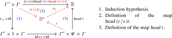
  By the induction hypothesis, $\sigma t\in , {{\mathbb {B}}^n}=\overline{, {\mathbb {B}}\times , {{\mathbb {B}}^{n-1}}}=\{u\mid u\longrightarrow ^*u_1\times u_2\text { with }u_1\in , {\mathbb {B}}\text { and }u_2\in , {{\mathbb {B}}^{n-1}}\}$. Hence, $\sigma (\text { head}\ t)=\text { head}\ \sigma t\longrightarrow ^*\text { head}(u_1\times u_2)\longrightarrow u_1\in , {\mathbb {B}}$.

• 

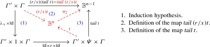
  By the induction hypothesis, $\sigma t\in , {{\mathbb {B}}^n}=\overline{, {\mathbb {B}}\times , {{\mathbb {B}}^{n-1}}}=\{u\mid u\longrightarrow ^*u_1\times u_2\text { with }u_1\in , {\mathbb {B}}\text { and }u_2\in , {{\mathbb {B}}^{n-1}}\}$. Hence, $\sigma (\text { tail}\ t)=\text { tail}\ \sigma t\longrightarrow ^*\text { tail}(u_1\times u_2)\rightarrow u_2\in , {{\mathbb {B}}^{n-1}}$.

• 

  By the induction hypothesis, we have that $\sigma t\in , {S(S\varPsi \times \varPhi )}$. Therefore, $\sigma t\in \overline{S(\overline{\overline{S, \varPsi }\times , \varPhi })}$.

  Hence, $\sigma t\longrightarrow ^*\sum _i\alpha _i ( (\sum _{j_i}\beta _{ij_i}r_{ij_i}) \times u_i)$ with $u_i\in , \varPhi$ and $r_{ij_i}\in , \varPsi$.

  Hence, $\Uparrow _r t\longrightarrow ^*\sum _{j_i}(\alpha _i\beta _{ij_i})\Uparrow _r(r_{ij_i}\times u_i)\in , {S(\varPsi \times \varPhi )}$.

•       Analogous to previous case.

$\square$

References

Altenkirch, T., Grattage, J.: A functional quantum programming language. In: Proceedings of the 20th Annual IEEE Symposium on Logic in Computer Science (LICS), pp. 249–258. IEEE (2005)
Arrighi, P., Dowek, G.: Lineal: a linear-algebraic lambda-calculus. Logical Methods in Computer Science 13(1:8) (2017)
Assaf, A., Díaz-Caro, A., Perdrix, S., Tasson, C., Valiron, B.: Call-by-value, call-by-name and the vectorial behaviour of the algebraic \(\lambda \)-calculus. Logical Methods in Computer Science 10(4:8) (2014)
Benton, N.: A mixed linear and non-linear logic: proofs, terms and models. In: Pacholski, L., Tiuryn, J. (eds.) Computer Science Logic (CSL 1994). Lecture Notes in Computer Science, vol. 933, pp. 121–135. Springer, Berlin (1994)
Borceux, F.: Handbook of Categorical Algebra, Encyclopedia of Mathematics and Applications, vol. 50. Cambridge University Press, Cambridge (2008)
Dascalescu, S., Nastasescu, C., Raianu, S.: Hopf Algebras: an Introduction. Pure and Applied Mathematics. A Series of Monographs and Textbooks. CRC Press, Boca Raton (2000)
Díaz-Caro, A., Dowek, G.: Typing quantum superpositions and measurement. Theory and Practice of Natural Computing (TPNC 2017). Lecture Notes in Computer Science, vol. 10687, pp. 281–293. Springer, Cham (2017)
Díaz-Caro, A., Dowek, G., Rinaldi, J.: Two linearities for quantum computing in the lambda calculus. BioSystems 186, 104012 (2019)
Díaz-Caro, A., Guillermo, M., Miquel, A., Valiron, B.: Realizability in the unitary sphere. In: Proceedings of the 34th Annual ACM/IEEE Symposium on Logic in Computer Science (LICS 2019), pp. 1–13 (2019)
Díaz-Caro, A., Malherbe, O.: A concrete categorical semantics for Lambda-\({\cal{S}}\). In: Logical and Semantic Frameworks with Applications (LSFA’18), Electronic Notes in Theoretical Computer Science, vol. 344, pp. 83–100 (2019)
Díaz-Caro, A., Malherbe, O.: A fully abstract model for quantum controlled lambda calculus. Draft at arXiv:1806.09236 (2020)
Díaz-Caro, A., Martínez, G.: Confluence in probabilistic rewriting. In: Logical and Semantic Frameworks with Applications (LSFA 2017), Electronic Notes in Teoretical Computer Science, vol. 338, pp. 115–131 (2018)
Ehrhard, T., Regnier, L.: The differential lambda-calculus. Theor. Comput. Sci. 309(1), 1–41 (2003)
Girard, J.Y.: Linear logic. Theor. Comput. Sci. 50, 1–102 (1987)
Girard, J.Y., Taylor, P., Lafont, Y.: Proofs and Types. Cambridge University Press, Cambridge (1989)
Grunenfelder, L., Paré, R.: Families parametrized by coalgebras. J. Algebra 107(2), 316–375 (1987)
Haim, M., Malherbe, O.: Linear hyperdoctrines and comodules. arXiv:1612.06602 (2016)
Kelly, G.: Doctrinal Adjunction. Category Seminar, Lectures Notes in Mathematics 420, 257–280 (1974)
Mac Lane, S.: Categories for the Working Mathematician, 2nd edn. Springer, Berlin (1998)
Tait, W.W.: Intensional interpretations of functionals of finite type I. J. Symb. Log. 32(2), 198–212 (1967)
Vaux, L.: The algebraic lambda calculus. Math. Struct. Comput. Sci. 19, 1029–1059 (2009)
Acknowledgements
We thank the anonymous reviewer for the suggestion with some examples on concrete models.
Author information
Authors and Affiliations
Corresponding author
Additional information
Communicated by Thomas Streicher.
Publisher's Note
Springer Nature remains neutral with regard to jurisdictional claims in published maps and institutional affiliations.
A. Díaz-Caro has been partially supported by PICT 2015 1208, ECOS-Sud A17C03 QuCa and PEDECIBA. O. Malherbe has been partially supported by MIA CSIC UdelaR.