Guided Search 6.0: An updated model of visual search

Abstract

This paper describes Guided Search 6.0 (GS6), a revised model of visual search. When we encounter a scene, we can see something everywhere. However, we cannot recognize more than a few items at a time. Attention is used to select items so that their features can be “bound” into recognizable objects. Attention is “guided” so that items can be processed in an intelligent order. In GS6, this guidance comes from five sources of preattentive information: (1) top-down and (2) bottom-up feature guidance, (3) prior history (e.g., priming), (4) reward, and (5) scene syntax and semantics. These sources are combined into a spatial “priority map,” a dynamic attentional landscape that evolves over the course of search. Selective attention is guided to the most active location in the priority map approximately 20 times per second. Guidance will not be uniform across the visual field. It will favor items near the point of fixation. Three types of functional visual field (FVFs) describe the nature of these foveal biases. There is a resolution FVF, an FVF governing exploratory eye movements, and an FVF governing covert deployments of attention. To be identified as targets or rejected as distractors, items must be compared to target templates held in memory. The binding and recognition of an attended object is modeled as a diffusion process taking > 150 ms/item. Since selection occurs more frequently than that, it follows that multiple items are undergoing recognition at the same time, though asynchronously, making GS6 a hybrid of serial and parallel processes. In GS6, if a target is not found, search terminates when an accumulating quitting signal reaches a threshold. Setting of that threshold is adaptive, allowing feedback about performance to shape subsequent searches. Simulation shows that the combination of asynchronous diffusion and a quitting signal can produce the basic patterns of response time and error data from a range of search experiments.

Introduction

Visual search has been a major topic of research for decades. There are a number of reasons for this. To begin, we spend a great deal of time doing search tasks. Many of these are so fast and seemingly trivial that we don’t tend to think of them as searches. Think, for example, about eating dinner. You search for the fork, then the potatoes, then the salt, then the potatoes again, then your drink, then the napkin, and so forth. As you drive, you look for specific items like the exit sign at the same time as you are searching for broad categories like “danger.” In more specialized realms, radiologists search images for signs of cancer, transportation security officers search carry-on baggage for threats, and so forth. Search is a significant, real-world task. At the same time, it has proven to be a very productive experimental paradigm in the lab. In a classic laboratory search task, observers might be asked to look for a target that is present on 50% of trials among some variable number of distractors. The number of items in the display is known as the “set size” and very systematic and replicable functions relate response time (or “reaction time,” RT in either case) and/or accuracy to that set size (Wolfe, 2014).

For some tasks (as shown in Fig. 1a and b), the number of distractors has little or no impact. The target seems to simply “pop-out” of the display (Egeth, Jonides, & Wall, 1972) and, indeed, may “capture” attention, even if it is not the target of search (Jonides & Yantis, 1988; Theeuwes, 1994). The slope of the RT x set size functions will be near (but typically a little greater than) 0 ms/item (Buetti, Xu, & Lleras, 2019). For other tasks, the time required to find the target increases (typically, more or less linearly) with the set size. In some cases, this reflects underlying limits on visual resolution. Thus, if the task is to find “TLT” among other triplets composed of Ts and Ls, a combination of acuity and crowding limits (Levi, Klein, & Aitsebaomo, 1985; Whitney & Levi, 2011) will require that each triplet be foveated in series until the target is found or the search is abandoned (Fig. 1c and d). Since the eyes fixate on three to four items per second, the slope of the RT x set size functions will be ~250–350 ms/item for target-absent trials (when all items need to be examined in order to be sure that the target is not present). Slopes for target-present trials will be about half that because observers will need to examine about half of the items on average before stumbling on the target. Figure 1e and f show a more interesting case. Here the target, a digital “2,” is presented among digital 5s. The items are large and the display sparse enough to avoid most effects of crowding. Nevertheless, slopes of the target-absent trials will tend to be around 90 ms/item on absent trials and, again, about half that on target-present trials (Wolfe, Palmer, & Horowitz, 2010). This will be true, even if the eyes do not move (Zelinsky & Sheinberg, 1997).

Fig. 1

Basic laboratory search tasks and reaction time (RT) x set size graphs

These patterns in the data were uncovered in the 1960s and 1970s (Kristjansson & Egeth, 2020) and formed the basis of Anne Treisman’s enduringly influential Feature Integration Theory (FIT) (Treisman & Gelade, 1980). Building on an architecture proposed by Neisser (1967), Treisman held that there was an initial, “preattentive” stage of processing, in which a limited set of basic features like color and orientation could be processed in parallel across the visual field. In this, she was inspired by the then-novel physiological findings showing cortical cells and areas that appeared to be specialized for these features (e.g., Zeki, 1978). In behavioral experiments, a unique feature, if it was sufficiently different from its neighbors, would pop-out and be detected, independent of the number of distractor items.

Basic features might be processed in parallel in separate cortical maps, but we do not see separate features. We see objects whose features are bound together. Treisman proposed that this “binding” required selective attention to connect isolated features to a single representation (Roskies, 1999; Treisman, 1996; Wolfe & Cave, 1999). This attention was capacity limited, meaning that only one or a very few items could be attended and bound at any given time. As a result, while a salient unique feature could be found in parallel, all other types of targets would require serial, selective attention from item to item. This proposed serial/parallel dichotomy and FIT more generally have proven to be extremely influential and persistent (~14,000 citations for Treisman & Gelade, 1980, in Google Scholar at last check).

Influential or not, it became clear over the course of the 1980s that FIT was not quite correct. The core empirical challenge came from searches for conjunctions of two features. For example, observers might be asked to search for a red vertical target among red horizontal and green vertical distractors. Identification of this target would require binding of color and orientation and, thus, it should require serial search. However, it became clear that conjunction searches were often more efficient than FIT would predict (Egeth, Virzi, & Garbart, 1984; McLeod, Driver, & Crisp, 1988; Nakayama & Silverman, 1986; Quinlan & Humphreys, 1987; Wolfe, Cave, & Franzel, 1989). The explanation can be illustrated by a version of a conjunction search used by Egeth, Virzi, and Garbart (1984). If we return to Fig. 1e–f, suppose you knew that the “2” was purple. It should be intuitively obvious that, while search may still be necessary, it will be unnecessary to attend to green items. If just half the items are purple, then just half the items are relevant to search and the slopes of the RT x set size functions will be cut in half, relative to the case where there is no color information.

In 1989, Wolfe, Cave, and Franzel (1989) proposed that the preattentive feature information could be used to “guide” the serial deployment of attention; hence the name of the model, “Guided Search” (GS). The original version of GS was otherwise quite similar to FIT. The core difference was that, while FIT proposed a dichotomy between parallel and serial search tasks, GS proposed a continuum based on the effectiveness of guidance. Pop-out search (Fig. 1a and b) arose when preattentive feature information guided attention to the target the first time, every time. A search for a 2 among 5s would be unguided because both target and distractors contained the same basic features. Results for conjunction searches lay in between, reflecting different amounts of guidance.

Treisman recognized the problem with the original FIT and proposed her own accounts in subsequent papers (e.g., Treisman & Sato, 1990). It was a subject of some annoyance to her that she continued to get taken to task for theoretical positions that she no longer held. Indeed, to this day, 40 years after FIT appeared, a simple two-stage, parallel-serial dichotomy is asserted in textbooks and by many research papers, especially outside the core disciplines of Experimental Psychology/Cognitive Science. To avoid this fate, when the time came to revise Guided Search in the light of new research, the paper was entitled “Guided Search 2.0: A revised model of visual search” (Wolfe, 1994a). Subsequent revisions have also been given version numbers. GS2 remains the most cited of the versions. GS3 (Wolfe & Gancarz, 1996) was something of a dead end, and GS4 (Wolfe, 2007) was published as a book chapter and, thus, less widely known. GS5 (Wolfe, Cain, Ehinger, & Drew, 2015) did not get beyond being a conference talk before being derailed by new data. The goal of the present paper is to describe Guided Search 6 (GS6). Since GS2 is the best known version of GS, this paper will frame GS6 in terms of the major changes from GS2. GS6 is needed because we know a lot more about search than we knew in 1980 or 1994. Still, this model presented here is an evolution and not a repudiation of the core ideas of FIT and the earlier versions of GS. Though some would disagree (Di Lollo, 2012; Hulleman & Olivers, 2017; Kristjansson, 2015, Zelinsky et al., 2020), the basic ideas from 40 years ago have proven very durable.

Guided Search 2.0

Figure 2 offers an illustration of GS2. The numbers are referred to in the summary of the key ideas, presented below:

• 1. Information from the world….

• 2. … is represented in the visual system. The nature of that representation will depend on the position of items in the visual field, properties of early visual channels, etc. In the early stages of processing, this will involve extraction of information about basic features like color and orientation.

• 3. Capacity limitations require that many activities, notably object recognition, can only be performed on one or a very few items at a time. Thus, there is a tight bottleneck that passes only the current object of attention for capacity-limited processing (e.g., “binding”).

• 4. An item, selected by attention, is bound, recognized, and tested to determine if it is a target or a distractor. If it is a match, search can end. If there are no matches, search will terminate when a quitting threshold (not diagrammed here) is reached.

• 5. Importantly, selection is rarely random. Access to the bottleneck is guided by a “priority map” that represents the system’s best guess as to where to deploy attention next. Attention will be deployed to the most active location on the map.

• 6. One source of priority map guidance comes from “bottom-up” salience: Salience is based on coarse representations of a limited number of basic features like color, size, etc. Bottom-up is defined as “stimulus-driven”.

• 7. Attentional priority is also determined by “top-down” guidance. “Top-down” guidance represents the implicit or explicit goals of the searcher. Top-down guidance is based on the basic features of the target as represented in memory. That is, if the observer was searching for a red vertical line, the red color and vertical orientation of that target could be used to guide attention.

• 8. Both of these sources of guidance are combined in a weighted manner to direct attention to the next item/location. If that item is a distractor, that location is suppressed (perhaps via “inhibition of return” (IOR; R. Klein, 1988)), and attention is deployed to the next highest peak on the map. This guided search continues until the target is found or the search terminates

  Fig. 2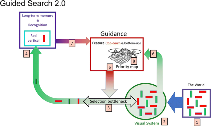

  

  A schematic representation of Guided Search 2.0.

From GS2 to GS6

The core ideas of GS have remained relatively constant over time, but new data require modifications of each of the main components: preattentive features, guidance, serial versus parallel processing, and search termination. In addition, the model requires consideration of topics that were not discussed in GS2; notably, the contribution of “non-selective” processing, the role of eccentricity (functional visual fields; FVFs), the role of non-selective processing (scene gist, ensembles, etc.), and the nature of the search template (or templates) and their relationship to working memory and long-term memory.

Here, in the same format as the GS2 diagram and description, Fig. 3 illustrates GS6. This diagram and description will introduce the topics for the bulk of the paper.

• 1. Information from the world is represented in the visual system. The nature of that representation will depend on the position in the visual field relative to fixation (eccentricity effects, crowding, etc.). Thus, an item near fixation will be more richly represented than one further away. These eccentricity constraints define one of three types of functional visual field (FVF) that are relevant for search (see #10, below).

• 2. Some representation of the visual input is available to visual awareness at all points in the field, in parallel, and via a non-selective pathway that was not considered in GS2. Thus, you see something everywhere. Ensemble statistics, scene gist, and other rapidly extracted attributes generally do not require selective attention and can be attributed to this non-selective pathway (Wolfe, Vo, Evans, & Greene, 2011).

• 3. There are capacity limits that require that many tasks can only be performed on one (or a very few) item/s at a time. Notably, for present purposes, this includes object recognition. Selective attention, as used here, refers to the processes that determine which items or regions of space will be passed through the bottleneck. Items are selected by attention at a rate of ~20 Hz, though this will vary with task difficulty (Wolfe, 1998).

• 4. Access to the bottleneck (i.e., attentional selection) is “guided” (hence Guided Search).

• 5. In GS6, there are five types of guidance that combine to create an attentional “Priority Map.” Bottom-up (salience) and top-down (user/template-driven) guidance by preattentive visual features are retained from all previous versions of GS. Newer data support guidance by the history of prior attention (e.g., priming), value (e.g., rewarded features), and, very importantly, guidance from the structure and meaning of scenes.

• 6. The selected object of attention is represented in working memory (speculatively, the limits on what can be selected at any given time may be related to the limits on the capacity of WM). The contents of WM can prime subsequent deployments of attention. WM also holds the top-down “guiding template” (i.e., the template that guides toward target attributes like “yellow” and “curved” if you are looking for a banana).

• 7. A second template is held in “activated long-term memory” (ALTM), a term referring to a piece of LTM relevant to the current task. This “target template” can be matched against the current object of attention in WM in order to determine if that object of attention is a target item. Thus, the target template is used to determine that this item is not just yellow and curved. Is it, in fact, the specific banana that is being looked for? In contrast to the one or two guiding templates in WM, ALTM can hold a very large number of target templates (as in Hybrid Search tasks having as many as 100 possible targets (Wolfe, 2012)). Those target templates might be highly specific (this banana in this pose) or much more general (e.g., any fruit).

• 8. The act of determining if an item, selected by attention, and represented in WM, is a target can be modeled as a diffusion process, with one diffuser for every target template that is held in ALTM. If a target is found, it can be acted upon.

• 9. A separate diffuser accumulates toward a quitting threshold. This will, eventually, terminate search if a target is not found before the quitting threshold is reached.

• 10. Not shown: In addition to a resolution Functional Visual Field (FVF), mentioned in #1 above, two other FVFs govern search. An attentional FVF governs covert deployments of attention during a fixation. That is, if you are fixated at one point, your choice of items to select is constrained by this attentional FVF. An explorational FVF constrains overt movements of the eyes as they explore the scene in search of a target

  Fig. 3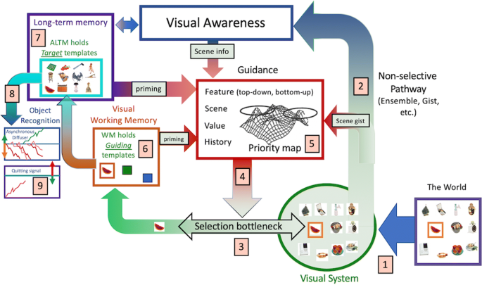

  

  A schematic representation of Guided Search 6.0.

A short-hand for capturing the main changes in GS6 might be that there are now two pathways, two templates, two diffusion mechanisms, three FVFs, and five sources of guidance. The paper is divided into six sections: (1) Guidance, (2) The search process, (3) Simulation of the search process, (4) Spatial constraints and functional visual fields, (5) Search templates, and 6) Other search tasks.

Five forms of guidance

In this section, we review the two “classic” forms of guidance: top-down and bottom-up feature guidance. Then we argue for the addition of three other types of guidance: history (e.g., priming), value, and, the most important of these, scene guidance. The division of guidance into exactly five forms is less important than the idea that there are multiple sources of guidance that combine to create an attention-directing landscape here called a “priority map.”

What do we know about classic top-down and bottom-up guidance by preattentive features?

To begin, “preattentive” is an unpopular term in some circles; in part, because it can be used, probably incorrectly, to propose that some pieces of the brain are “preattentive” or to propose that preattentive processing occurs for the first N ms and then ends. The term is useful in the following sense. If we accept the existence of selective attention and if we accept that, by definition, we cannot selectively attend to everything at once, it follows that, when a stimulus appears, some aspects have not been selected yet. To the extent that they are being processed, that processing is tautologically preattentive. A stimulus feature that can be processed in this way is, thus, a preattentive feature. This is not the end of the discussion. For instance, if an item is attended and then attention is deployed elsewhere, is its “post-attentive” state similar to its preattentive state (Rensink, 2000; Wolfe, Klempen, & Dahlen, 2000)? For the present, if selective attention is a meaningful term, then preattentive is a meaningful term as well. Some information (e.g., aspects of texture and scene processing) can be thought of as “non-selective” (Wolfe et al., 2011) in the sense that, not only are they available before attentional selection but they have an impact on visual awareness without the need for attentional selection.

Preattentive feature guidance

A preattentive feature is a property capable of guiding the deployment of attention. These features are derived from but are not identical to early visual processing stages. Orientation serves as a clear example of the difference between early vision (#1 in Fig. 3) and preattentive guidance (#5) because it has been the subject of extensive research. For instance, early visual processes allow for very fine differentiation of the orientation of lines. A half-degree tilt away from vertical is not hard to detect (Olzak & Thomas, 1986). That detectable difference will not guide attention. The difference between an item and its neighbors must be much greater if an attention-guiding priority signal is to be generated (roughly 10–15°. It will depend on the stimulus parameters; see Foster & Ward, 1991a, 1991b; Foster & Westland, 1998). Similar effects occur in color (Nagy & Sanchez, 1990) and, no doubt, they would be found in other features if tested. Guidance is based on a coarse representation of a feature. That coarse representation is not simply the fine representation divided by some constant. Using orientation, again, as an example, geometrically identical sets of orientations do not produce identical guidance of attention. The categorical status of the items is important. Thus, a -10° target among +50 and -50° distractors is easier to find than a 10° target among -30° and 70° distractors. The second set of lines is simply a 20° rotation of the first. Thus, the angular relations between the target and distractor lines are the same. However, in the first set, the target is the only steep line whereas in the second set, it is merely the steepest (Wolfe, Friedman-Hill, Stewart, & O'Connell, 1992). A target of a unique category is easier to find (see also Kong, Alais, & Van der Berg, 2017). Again, there are similar effects in color (Nagy & Sanchez, 1990).

Fine discriminations, like the discrimination that half degree tilt from vertical, rely on information encoded in early vision and require attention. This can be seen as an example of re-entrant processing (Di Lollo, Enns, & Rensink, 2000) and/or support for the Reverse Hierarchy Theory (Hochstein & Ahissar, 2002). In both cases, the idea is that attention makes it possible to reach down from later stages of visual processing of the visual system to make use of fine-grain information represented in early vision.

Preattentive guidance is complex

It would be lovely if top-down and bottom-up feature guidance could be calculated in a straight-forward manner from the stimulus, using rules that generalize across different featural dimensions. Bottom-up salience maps are based on something like this assumption (e.g., Bisley & Mirpour, 2019; Itti & Koch, 2000; Li, 2002) and, certainly, there are important general rules. Duncan and Humphreys (1989) gave a clear articulation of some of the most basic principles. In general, guidance to a target will be stronger when the featural differences between the target (T) and distractor (D) are larger (TD differences), and guidance to a target will be stronger when the featural differences amongst distractors are smaller (DD similarity). Other more quantitative rules about combining signals across features are appearing (Buetti et al., 2019; Lleras et al., 2020). That said, TD and DD distances are not simple functions of the distance from the one feature value to another in some unit of the physical stimulus or some unit of perceptual discriminability like a just noticeable difference (Nagy & Sanchez, 1990; Nagy, Sanchez, & Hughes, 1990). Moreover, it is an unfortunate fact that rules that apply to one guiding feature do not necessarily apply to another guiding feature, or even to the same feature in a different situation. For example, it seems quite clear that color and orientation both guide attention in simple searches for conjunctions of color and orientation (e.g., Friedman-Hill & Wolfe, 1995). One would like to imagine that any time that half of the items in a display had a guiding feature like a specific color or orientation, the other half of the items would be treated as irrelevant to search. However, that does not appear to be consistently true. Orientation information can fail to guide and can even make search less efficient (Hulleman, 2020; Hulleman, Lund, & Skarratt, 2019). When guidance is provided by previewing one feature, different features (color, size, orientation) can show very different patterns of guidance, even if the feature differences have been equated (Olds & Fockler, 2004). Here, too, orientation information can actually make search less efficient. For modeling purposes, using basic salience measures and basic rules about TD and DD similarity is a decent approximation but not a full account.

Preattentive processing takes time

Earlier versions of GS (and other accounts of feature guidance) tended to treat the preattentive, feature-processing stage as a single, essentially instantaneous step in which the features were processed in parallel across the entire stimulus. If the target was “red” and “vertical,” that color and orientation information was immediately available in a priority map, ready to guide attention. That is not correct. Palmer et al. (2019) showed that it takes 200–300 ms for even very basic guidance by color to be fully effective. Lleras and his colleagues (2020) have produced important insights into the mechanics of this “parallel,” “preattentive” stage of processing in a series of experiments that show that RTs in basic feature searches increase with the log of the set size. Even the most basic of feature searches do not appear to have completely flat, 0 ms/item slopes (Buetti, Cronin, Madison, Wang, & Lleras, 2016; Madison, Lleras, & Buetti, 2018). Lleras et al. (2020) offer an interesting account of the cause of this log function in their “target contrast signal theory (TCS)”. They argue that a diffusion process (Ratcliff, 1978) accumulates information about the difference between each item and the designated target. Other diffusion models (including GS, see below) typically ask how long it takes for information to accumulate to prove that an item is a target. TCS emphasizes how long it takes to decide that attention does not need to be directed to a distractor item. The TCS model envisions a preattentive stage that ends when all the items that need to be rejected have been rejected. The remaining items (any targets as well as other “lures” or “candidates”) are then passed to the next stage. Since diffusion has a random walk component, some items will take longer than others to finish. Leite and Ratcliff (2010) have shown that the time required to end a process with multiple diffusers will be a log function of the number of diffusers and, in TCS, this explains the log functions in the data. In more recent work, Heaton et al. (2020) make the important point that it is a mistake to think of preattentive processing as something that stops after some time has elapsed. Preattentive and/or non-selective processing must be ongoing when a stimulus is visible. Deployment of attention will be dependent on the priority map generated by the current state of that preattentive processing and that current state will be continually evolving especially as the eyes and/or the observer move.

TCS does not explain some important aspects of preattentive processing (nor is it intended to do so). For example, what is happening when the target is simply an odd item that “pops-out” because it is unique? Thus, in Fig. 4 (which we discuss for other purposes later), the intended targets are orange. Nevertheless, attention is attracted to the blue items even though the blue items can be easily rejected as not orange. They are sufficiently different from their neighbors to attract attention in a “bottom-up,” stimulus-driven manner. Regardless, the TCS model and its associated data make the clear point that the preattentive processing stage will take some amount of time and that this time will be dependent on the number of items in the display, even if all items are processed in parallel.

Fig. 4

Feature search based on bottom-up salience, top-down relations, and top-down identity

TCS also raises the possibility that guidance could be as much about rejecting distractors as it is about guiding toward targets (Treisman and Sato, 1990); a topic that has seen a recent burst of interest (e.g., Conci, Deichsel, Müller, & Töllner, 2019; Cunningham & Egeth, 2016; Stilwell & Vecera, 2019). In thinking about distractor rejection, it is important to distinguish two forms of rejection. One could reject items that do not have the target feature (e.g., in Fig. 4, reject items that are not orange) or one could reject items that have a known distractor feature (e.g., reject items that are red). Friedman-Hill and Wolfe (Exp. 4, 1995) and Kaptein, Theeuwes, and Van der Heijden (1995) found evidence that observers could not suppress a set of items on the basis of its defining feature. In a study of the priming effect, Wolfe, Butcher, Lee, and Hyle (2003) found that the effects of repeating target features were much greater than those of repeating distractors. Still, the distractor effects were present and subsequent work, suggests that distractor inhibition is a contributor to guidance even if it may take longer to learn and establish (Cunningham & Egeth, 2016; Stilwell & Vecera, 2020).

Feature guidance can be relational

Over the past decade, Stefanie Becker’s work has emphasized the role of relative feature values in the guidance of attention (Becker, 2010; Becker, Harris, York, & Choi, 2017). This is also illustrated in Fig. 4, where, on the left, the orange targets are the yellower items, while on the right, the same targets are the redder items. Attention can be guided by a filter that is not maximally sensitive to the feature(s) of the target. On the right side of Fig. 4, for example, it might be worth using a filter maximally sensitive to “red” even though the target is not red. The most useful filter will be the one that reveals the greatest difference between target and distractors (Yu & Geng, 2019). Targets and distractors that can be separated by a line, drawn in some feature space, are said to be “linearly separable” (Bauer, Jolicoeur, & Cowan, 1998; Bauer, Jolicoeur, & Cowan, 1996). If, as in the middle of Fig. 4, no line in color space separates targets and distractors, search is notably more difficult (look for the same orange squares). Some of this is due to the inability to use Becker’s relational guidance when targets are not linearly separable from distractors, and some of the difficulty is due to added bottom-up (DD similarity) noise produced by the highly salient contrast between the two types of yellow and red distractors. Note, however, that attention can still be guided to the orange targets, showing that top-down guidance is not based entirely on a single relationship (for more, see Kong, Alais, & Van der Berg, 2016; Lindsey et al., 2010). Moreover, Buetti et al. (2020) have cast doubt on the whole idea of linear separability, arguing that performance in the inseparable case can be explained as a function of performance on each of the component simple feature searches. In their argument, the middle of Fig. 4 would be explained by the two flanking searches without the need for an additional effect of linear separability.

Spatial relations are at least as important as featural relations in feature guidance. Figure 5 illustrates this point using density. In the figure, the orange targets and yellow distractors on the left are the same as those on the right but those orange targets are less salient and guide attention less effectively because they are not as physically close to the yellow distractors (Nothdurft, 2000). An interesting side effect of density is that the RT x set size function can become negative if increasing density speeds the search more than the set size effect slows search (Bravo & Nakayama, 1992).

Fig. 5

Density effects in search: Feature differences are easier to detect when items are closer together

Feature Guidance is modulated by position in the visual field

GS2, following Neisser (1967) says “there are parallel processes that operate over large portions of the visual field at one time” (Wolfe, 1994a, p.203). However, it is important to think more carefully about the spatial aspects of guidance and preattentive processing.

The visual field is not homogeneous. Of course, we knew this with regard to attentive vision and object recognition. As you read this sentence, you need to fixate one word after another, because acuity falls off with distance from the fovea, the point of fixation (Olzak & Thomas, 1986). Moreover contours “crowd” each other in the periphery, making them still harder to perceive correctly (Levi, 2008). Thus, you simply cannot read words of a standard font size more than a small distance from fixation. What must be true but is little remarked on, is that preattentive guidance of attention must also be limited by eccentricity effects.

In Fig. 6, look at the star and report on the color of all the ovals that you can find. Without moving your eyes, you will be able to report the purple oval at about 4 o’clock and the blue isolated oval at 2 o’clock. The same preattentive shape/orientation information that guides your attention to those ovals will not guide your attention to the other two ovals unless you move your eyes. Thus, while preattentive processing may occur across large swaths of the visual field at the same time, the results of that processing will vary with eccentricity and with the structure of the scene. In that vein, it is known that there are eccentricity effects in search. Items near fixation will be found more quickly and these effects can be neutralized by scaling the stimuli to compensate for the effects of eccentricity (Carrasco, Evert, Chang, & Katz, 1995; Carrasco & Frieder, 1997; Wolfe, O'Neill, & Bennett, 1998).

Fig. 6

Look at the star and report the color of ovals

Thinking about search in the real world of complex scenes, it is clear that the effects of eccentricity on guidance are going to be large and varied. Returning to Fig. 6, for example, both color and shape are preattentive features but guidance to “oval” will fail at a much smaller eccentricity than guidance to that one “red” spot. Rosenholtz and her colleagues attribute the bulk of the variation in the efficiency of search tasks to the effects of crowding and the loss of acuity in the periphery (Rosenholtz, Huang, & Ehinger, 2012; Rosenholtz, 2011, 2020; Zhang, Huang, Yigit-Elliott, & Rosenholtz, 2015). Guided Search isn’t prepared to go that far, but it is clear that crowding and eccentricity will limit preattentive guidance. Those limits will differ for different features in different situations, but this topic is vastly understudied. We will return to these questions in the later discussion of the functional visual field (FVF). For the present, it is worth underlying the thought that preattentive guidance will vary as the eyes move in any normal, real world search.

Levels of selection: Dimensional weighting

Though guidance is shown as a single box (#5 in Fig. 3) controlling access to selective processing (#4), it is important to recognize that selection is a type of attentional control, not one single thing. We have been discussing guidance to specific features (e.g., blue … or bluest), but attention can also be directed to a dimension like color. This “dimension weighting” has been extensively studied by Herman Muller and his group (reviewed in Liesefeld, Liesefeld, Pollmann, & Müller, 2019; Liesefeld & Müller, 2019). Their “dimension-weighting account” (DWA) is built on experiments where, for example, the observer might be reporting on some attributes of a green item in a field of blue horizontal items. If there is a salient red “singleton” distractor, it will slow responses more than an equally salient vertical distractor. DWA argues that a search for green puts weight on the color dimension. This results in more distraction from another color than from another dimension like orientation.

At a level above dimensions, observers can attend to one sense (e.g., audition) over another (e.g., vision). As any parent can attest, their visual attention to the stimuli beyond the windshield can be disrupted if their attention is captured by the auditory signals from the back seat of the car.

Building the priority map – Temporal factors and the role of “attention capture”

In Guided Search, attention is guided to its next destination by a winner-take-all operation (Koch & Ullman, 1985) on an attentional priority map (Serences & Yantis, 2006). In GS2, the priority map was modeled as a weighted average of contributions from top-down and bottom-up processing of multiple basic features. In GS6, there are further contributions to priority, as outlined in the next sections. In thinking about the multiple sources of guidance, it is worth underlining the point made earlier, that the priority map is continuously changing and continuously present during a search task. Different contributions to priority have different temporal properties. Bottom-up salience, for instance, may be a very powerful but short-lived form of guidance (Donk & van Zoest, 2008). Theeuwes and his colleagues (Theeuwes, 1992; Van der Stigchel, et al., 2009), as well as many others (e.g., Harris, Becker, & Remington, 2015; Lagroix, Yanko, & Spalek, 2018; Lamy & Egeth, 2003), have shown that a salient singleton will attract attention. Indeed, there is an industry studying stimuli that “capture” attention (Folk & Gibson, 2001; Theeuwes, Olivers, & Belopolsky, 2010; Yantis & Jonides, 1990). Donk and her colleagues have argued that this form of guidance is relatively transient in experiments using artificial stimuli (Donk & van Zoest, 2008) and natural scenes (Anderson, Ort, Kruijne, Meeter, & Donk, 2015). Others have shown that the effects may not completely vanish in the time that it takes to make a saccade (De Vries, Van der Stigchel, Hooge, & Verstraten, 2017), but this transient nature of bottom-up salience may help to explain why attention does not get stuck on high salience, non-target spots in images (Einhauser, Spain, & Perona, 2008). Lamy et al. (2020) make the useful point that “attention capture” may be a misnomer. It might be better to think that stimuli for attention capture create bumps in the priority map. In many capture designs, that bump will be the winner in the winner-take-all competition for the next deployment of attention. However, other capture paradigms may be better imagined as changing the landscape of priority, rather than actually grabbing or even splitting the “spotlight” of attention (Gabbay, Zivony, & Lamy, 2019).

The landscape of priority can be modulated in a negative/inhibitory manner as well. Suppose that one is searching for blue squares among green squares and blue circles. This conjunction search can be speeded if one set of distractors (e.g., all the green squares) is shown first. This is known as “visual marking” and is thought to reflect some reduction in the activation of the previewed items (Watson & Humphreys, 1997). One could conceive of marking as a boost to the priority of the later stimuli, rather than inhibition (Donk & Theeuwes, 2003; but see Kunar, Humphreys, and Smith, 2003). For present purposes, the important point is that marking shows that priority can evolve over time. Subsequent work has shown the limits on that evolution. If there is enough of a break in the action, the map may get reset (Kunar, Humphreys, Smith, & Hulleman, 2003; Kunar, Shapiro, & Humphreys, 2006). If we think about priority maps in the real world or in movies, it would be interesting to see if the maps are reset by event boundaries (Zacks & Swallow, 2007).

Expanding the idea of guidance – history effects

As the phenomenon of marking suggests, the priority map is influenced by several forms of guidance other than the traditional top-down and bottom-up varieties. To quote Failing and Theeuwes (2018); “Several selection biases can neither be explained by current selection goals nor by the physical salience of potential targets. Awh et al. (2012) suggested that a third category, labeled as “selection history”, competes for selection. This category describes lingering selection biases formed by the history of attentional deployments that are unrelated to top-down goals or the physical salience of items.” (Failing & Theeuwes, 2018, p.514). There are a variety of effects of history. We are dividing these into two forms of guidance. We will use the term “history” effects to refer to the effects that arise from passive exposure to some sequence of stimuli (e.g., priming effects). In contrast, “value” or “reward” effects are those where the observer is learning to associate positive or negative value to a feature or location. This distinction is neither entirely clear nor vitally important. These phenomena represent ways to change the landscape of the priority map that are not based on salience or the observer’s goals. One classic form of the priming variety of history effects is the “priming of pop-out” phenomenon of Maljkovic and Nakayama (1994). In an extremely simple search for red among green and vice versa, they showed that RTs were speeded when a red target on trial N followed red on trial N-1 (or green followed green). Theeuwes has argued that all feature-based attention can be described as priming of one form or another (Theeuwes, 2013; Theeuwes, 2018). This seems a bit extreme. After all, you can guide your attention to all the blue regions in your current field of view without having been primed by a previous blue search. Top-down guidance to blue would seem to be enough (see Leonard & Egeth, 2008). Nevertheless, the previous stimulus clearly exerts a force on the next trial. In the “hybrid foraging” paradigm, where observers (Os) search for multiple instances of more than one type of target, they are often more likely to collect two of the same target type in a row (run) than they are to switch to another target type (Kristjánsson, Thornton, Chetverikov, & Kristjansson, 2018; Wolfe, Aizenman, Boettcher, & Cain, 2016). These runs are, no doubt, partially due to priming effects. Introspectively, when the first instance of a target type is found in a search display containing multiple instances, those other instances seem to “light up” in a way that suggests that finding the first one primed all the other instances, giving them more attentional priority.

Contextual cueing

Contextual cueing (Chun & Jiang, 1998) represents a different form of a history effect. In contextual cueing, Os come to respond faster to repeated displays than to novel displays, as if the Os had come to anticipate where the target would appear even though they had no explicit idea that the displays had been repeating (Chun, 2000). It has been argued that contextual cueing might just be a form of response priming (Kunar, Flusberg, Horowitz, & Wolfe, 2007). That is, Os might just be faster to respond when they find a target in a contextually cued location. However, the predominant view has been that contextual cueing represents a form of implicit scene guidance (see below) in which recognition of the scene (even implicitly) boosts the priority map in the likely target location (Sisk, Remington, & Jiang, 2019; Harris & Remington, 2020).

Value

A different route to modulation of priority comes from paradigms that associate value with target and/or distractor features. If you reward one feature (e.g., red) and/or punish another (e.g., green), items with rewarded features will attract more attention and items with punished features will attract less attention (Anderson, Laurent, & Yantis, 2011). As with contextual cueing, it could be argued that the effect of reward is to speed responses once the target is found, and not to guide attention to the target. However, Lee and Shomstein (2013) varied set sizes and found that value could make slopes shallower. This is an indication that value had its effects on the search process and not just on the response once a target is found. Moreover, the effects of reward can be measured using real scenes (Hickey, Kaiser, & Peelen, 2015), an indication that value can be a factor in everyday search.

We are labeling “history” and “value” as two types of guidance. One could further divide these and treat each paradigm (e.g., contextual cueing) as a separate type of guidance or, like Awh et al. (2012), one could group all these phenomena into “selection history.” Alternatively, priming, contextual cueing, value, marking, etc. could all be seen as variants top-down guidance. Bottom-up guidance is driven by the stimulus. Top-down guidance would be guidance with its roots in the observer. This was the argument of Wolfe, Butcher, Lee, and Hyle (2003) and of prior versions of GS. GS6 accepts the logic of Awh, Belopolsky, and Theeuwes (2012). Top-down guidance represents what the observer wants to find. History and value guidance show how the state of the observer influences search, independent of the observer’s intentions. Again, the important point is that there are multiple modulators of the landscape of attentional priority beyond top-down and bottom-up guidance.

Scene guidance

Selection history makes a real contribution to attentional guidance. However, these effects seem quite modest if compared to “scene guidance,” the other addition to the family of attention-guiding factors in GS6. Guidance by scene properties was not a part of earlier forms of Guided Search, largely because scenes were not a part of the body of data being explained by the model. Given a literature that dealt with searching random arrays of isolated elements on a computer screen, there was not much to say about the structure of the scene (though we tried in Wolfe, 1994b). Of course, the real world in which we search is highly structured and that structure exerts a massive influence on search. In Fig. 7a, ask which box or boxes are likely to hide a sheep. Unlike a search for a T amongst a random collection of Ls, where every item is a candidate target, there are sources of information in this scene that rapidly label large swathes of the image as “not sheep.”

Fig. 7

(a) Which boxes could hide a sheep? (b) Find sheep. The scene is on the grounds of Chatsworth House, a stately home in Derbyshire, England

Top-down guidance to sheep features is important here, but even with no sign of a sheep, scene constraints make it clear that “C” is a plausible location. Spatial layout cues indicate that any sheep behind “B” would be very small and “A,” “D,” and “E” are implausible, even though, looking at Fig. 7b, there are sheep-like basic features in the fluffy white clouds behind “E” and the bits in the building behind “D” that share color and rough shape with the sheep who was, in fact, behind “C.”

Like selection history, scene guidance is a term covering a number of different modulators of priority. Moreover, perhaps more dramatically than the other forms of guidance, scene guidance evolves over time. In Fig. 3, this is indicated by having two sources of scene information feeding into guidance. In the first moments after a scene becomes visible, the gist of the scene becomes available. Greene and Oliva (2009) demonstrated that exposures of 100 ms or less are all that are needed to permit Os to grasp the rough layout of the scene. Where is the ground plane? What is the rough scale of the space? A little more time gives the observer rough semantic information about the scene: Outdoors, rural, etc. For this specific example, very brief exposures are adequate to determine that there is likely to be an animal present (Li, VanRullen, Koch, & Perona, 2002; Thorpe, Fize, & Marlot, 1996), even if not to localize that animal (Evans & Treisman, 2005). Castelhano and her colleagues have formalized this early guidance by the layout in her Surface Guidance Framework (Pereira & Castelhano, 2019).

With time, other forms of scene guidance emerge. For example, Boettcher et al. (2018) have shown that “anchor objects” can guide attention to the location of other objects. Thus, if you are looking for a toothbrush, you can be guided to likely locations if you first locate the bathroom sink. Presumably, this form of scene guidance requires more processing of the scene than does the appreciation of the gist-like “spatial envelope” of the scene (Oliva, 2005). Since anchor objects are typically larger than the target object (sink -> toothbrush), this can be seen as related to the global-local processing distinction originally popularized by Navon (1977).

As one way to quantify scene guidance, Henderson and Hayes (2017) introduced the idea of a “meaning map.” A meaning map is a representation akin to the salience map that reflects bottom-up guidance of attention. To create a meaning map, Henderson and Hayes divided scenes up into many small regions. These were posted online, in isolation and in random order as a “Mechanical Turk” task in which observers were asked to rate the meaningfulness of each patch (i.e., a patch containing an eye might be rated as highly meaningful; a piece of wall, much less so). These results are summed together to form a heatmap showing where, in the scene, there was more or less meaning present. Meaning maps can predict eye movements better than salience maps calculated for the same images (Pedziwiatr, Wallis, Kümmerer, & Teufel, 2019). The method loses the valuable guiding signal from scene structure, but it is a useful step on the way to putting scene guidance on a similar footing with top-down and bottom-up guidance.

Rather like those classical sources of guidance, scene guidance may have a set of features, though these may not be as easy to define as color, size, etc. For example, in scene guidance, it is useful to distinguish between “syntactic” guidance – related to the physics of objects in the scene (e.g., toasters don’t float) and “semantic” guidance – related to the meaning of objects in the scene (e.g., toasters don’t belong in the bathroom; Biederman, 1977; Henderson & Ferreira, 2004; Vo & Wolfe, 2013).

Guidance summary

Guidance remains at the heart of Guided Search. Guidance exists to help the observer to deploy selective attention in an informed manner. The goal is to answer the question, “Where should I attend next?” The answer to that question will be based on a dynamically changing priority map, constructed as a weighted average of the various sources of guidance (see Yamauchi & Kawahara, 2020, for a recent example of the combination of multiple sources of guidance). The weights are under some explicit control. Top-down guidance to specific features is the classic form of explicit control (I am looking for something shiny and round). There must be an equivalent top-down aspect of scene guidance (I will look for that shiny round ball on the floor). There are substantial bottom-up, automatic, and/or implicit sources of guidance, particularly early in a search. Factors like salience and priming will lead to attentional capture early in a search. More extended searches must become more strategic to avoid perseveration (I know I looked for that shiny ball on the floor. Now I will look elsewhere). One way of understanding these changes over time is to realize that the priority map is continuously changing over time, and to be clear Treisman’s classic “preattentive” and “attentive” stages of processing are both active throughout a search.

Dividing guidance into five forms is somewhat arbitrary. There are different ways to lump or split guiding forces. One way to think about the forms of guidance that are added in GS6 (history, value, and scene) is that all of them can be thought of as long-term memory effects on search. They are learned over time: History effects on a trial-by-trial basis, value over multiple trials, and scene effects over a lifetime of experience. This role for long-term memory is somewhat different than the proposed role of activated long-term memory as the home of target templates in search, as is discussed later.

What are the basic features that guide visual search?

A large body of work describes the evidence that different stimulus features can guide search (e.g., color, motion, etc.). Other work documents that there are plausible features that do not guide search: for example, intersection type (Wolfe & DiMase, 2003) or surface material (Wolfe & Myers, 2010). A paper like this one would be an obvious place to discuss the evidence for each candidate feature, but this has been done several times recently (Wolfe, 2014, 2018; Wolfe & Horowitz, 2004; Wolfe & Horowitz, 2017), so the exercise will not be repeated here.

There are changes in the way we think about basic features in GS6. GS2 envisioned guiding features as coarse, categorical abstractions from the “channels” that define sensitivity to different colors, orientations, etc. (Wolfe et al., 1992). The simulation of GS2, for example, made use of some very schematic, broad color and orientation filters (see Fig. 3 of Wolfe, 1994a). This works well enough for relatively simple features like color or orientation (though some readers took those invented filters a bit too literally). It does not work well for more complex features like shape. It is clear that some aspects of shape guide attention and there have been various efforts to establish the nature of a preattentive shape space. Huang (2020) has proposed a shape space with three main axes: segmentability, compactness, and spikiness that seems promising. However, the problem becomes quite daunting if we think about searching for objects. Search for a distinctive real-world object in a varied set of other objects seems to be essentially unguided (Vickery, King, & Jiang, 2005). By this, we mean that the RT x set size functions for such a search look like those from other unguided tasks like the search for a T among Ls or a 2 among 5s (Fig. 1). On the other hand, a search for a category like “animal” can be guided. In a hybrid search task (Wolfe, 2012) in which observers had to search for any of several (up to 16) different animals, Cunningham & Wolfe (2014) found that Os did not attend to objects like flags or coins – presumably because no animals are that circular or rectangular. They did attend to distractors like clothing; presumably, because at a preattentive level, crumpled laundry has features that might appear to be sufficiently animal-like to be worth examining. But what are those features?

We would be hard-pressed to describe the category, “animal,” in terms of the presence or absence of classic preattentive features (e.g., What size is an animal, in general?). One way to think about this might be to imagine that the process of object recognition involves something like a deep neural network (DNN; Kriegeskorte & Douglas, 2018). If one is looking for a cow, finding that cow would involve finding an object in the scene that activates the cow node at the top of some many-layered object recognition network. Could some earlier layer in that network contain a representation of cow-like shape properties that could be used to guide attention in the crude manner that shape guidance appears to proceed? That is, there might be a representation in the network that could be used to steer attention away from books and tires, but would not exclude horses or, perhaps, bushes or piles of old clothes. This is speculative, but it is appealing to think that shape guidance might be a rough abstraction from the relatively early stages of the processes that perform object recognition, just as color guidance appears to be a relatively crude abstraction from the processes that allow you to assess the precise hue, saturation, and value of an attended color patch (Nagy & Cone, 1993; Wright, 2012).

The search process

In GS6, the search process is simultaneously serial and parallel

How does search for that cow proceed? The guidance mechanisms, described above, create a priority map based on a weighted average of all the various forms of guidance. Attention is directed to the current peak on that map. If it is the target and there is only one target, the search is done. If not, attention moves to the next peak until the target(s) is/are found and/or the search is terminated. Figure 8 shows how GS6 envisions this process.

Fig. 8

The search process in GS6.

Referring to the numbers in Fig. 8, (1) there is a search stimulus in the world; here a search for a T among Ls. (2) Items are selected from the visual system’s representation of that stimulus, in series. (3) Not shown, the choice of one item over another would be governed by the priority map, the product of the guidance processes, discussed earlier. (4) The selected item may be represented in Working Memory (Drew, Boettcher, & Wolfe, 2015). This will be discussed further, when the topic of the “search template” is considered. (5) The object of search is represented as a “Target Template” in Activated Long Term Memory (ALTM). Again, more will be said about templates, later. (6) Each selected item is compared to the target template by means of a diffusion process (Ratcliff, 1978; Ratcliff, Smith, Brown, & McKoon, 2016). It is not critical if this is strictly an asynchronous “diffusion” process, a “linear ballistic accumulator” (Brown & Heathcote, 2008), a “leaky accumulator” (Bogacz, Usher, Zhang, & McClelland, 2007), or another similar mechanism. There may be a correct choice to be made here but, for present purposes, all such processes have similar, useful properties, discussed below and there is good evidence that the nervous system is using such processes in search (Schall, 2019). Evidence accumulates toward a target boundary or a non-target boundary. (7) Distractors that reach the non-target boundary are “discarded.” The interesting question about those discarded distractors is whether they are irrevocably discarded or whether they can be selected again, later in the search. For example, in a foraging search like berry picking, one can imagine a berry, rejected at first glance, being accepted later on. In a search for a single target, successful target-present search ends when evidence from a target item reaches the target boundary (6).

Several questions about this process need to be addressed.

• 1) What is the purpose of an “asynchronous diffuser”?

• 2) What is the fate of rejected distractors and how do we avoid perseverating on a salient distractor object?

• 3) How is search terminated?

The Asynchronous Diffuser or The Carwash

The slope of RT x set size functions, like those in Fig. 1, can be thought of as a measure of the rate with which the search process, shown in Fig. 8, deals with items in the visual display. A task like the T versus L search, shown here, might produce target-present slopes of about 20–40 ms per item. For purposes of illustration, suppose that this T versus L search produces a target-present slope of 30 ms/item and further suppose, as Treisman would have proposed, that this is an unguided, serial, self-terminating search. If so, then observers would have to search through about half of the items, on average, before stumbling on the target. Taking this factor of 2 into account, if the target-present slope is 30 ms/item, the “true” rate would be about 60 ms/item or about 17 items per second moving through the system. Unfortunately, no one has developed an “attention tracker” that can monitor covert deployments of attention the way that an eye tracker can track overt deployments of the eyes so we cannot say for sure that attention is being discretely deployed in at the rate suggested by the slopes of RT x set size functions. There are useful hints that neural rhythms in the right frequency range are important to the neural basis of covert attention. For instance, Buschman and Miller (2009) could see monkeys shifting attention every 40 ms accompanied by local field potentials oscillating at 25 Hz. Lee, Whittington, and Kopell (2013) built a neural inspired model to show how oscillations in this beta rhythm range (18–25 Hz) could reproduce a variety of top-down attentional effects (see Miller & Buschman, 2013, for a review of this literature).

So, GS assumes that items are being selected one after the other and the data suggest that this is occurring at a rate of around 20 Hz. The problem is that no one seems to think that object recognition can take place in ~50 ms. Much more typical is the conclusion from an ERP study by Johnson and Olshausen (2003) that holds that recognition takes “between 150 and 300 ms.” Even papers proposing “ultra-rapid” recognition (VanRullen & Thorpe, 2001) are suggesting that imperfect but above chance performance takes 125–150 ms per object (Hung, Kreiman, Poggio, & DiCarlo, 2005; VanRullen & Thorpe, 2001). Thus, a model that proposes that items are selected and fully recognized every 50 ms is simply not plausible.

One solution has been to propose parallel processing of the display (Palmer & McLean, 1995; Palmer, Verghese, & Pavel, 2000) or, more recently, parallel processing of items in some region around fixation (see discussion of the functional visual field, below: Hulleman & Olivers, 2017). The GS6 solution, as illustrated in Fig. 8, is to propose that items may be selected to enter the processing pipeline every 50–60 ms or so, but that it may take several hundred milliseconds to move through the process to the point of recognition. As a consequence, at any given moment in search, multiple items will be in the diffusion/recognition process. Since they entered that process one after the other, the result is an asynchronous diffusion. A real-world analogy is a carwash (Moore & Wolfe, 2001; Wolfe, 2003). Cars enter and leave the carwash in a serial manner but multiple cars are being washed at the same time. Hence the process is neither strictly serial nor parallel. In computer science, this would be a pipeline architecture (Ramamoorthy & Li, 1977).

It is notoriously difficult to use behavioral data to distinguish serial processes from parallel processes (Townsend, 1971; Townsend, 2016). GS6 would argue that it is an essentially fruitless endeavor in visual search. The carwash/asynchronous diffuser is both serial and parallel. Moreover, it is easy to imagine variations on the carwash architecture of Fig. 8. Maybe two “cars” can enter at once. Maybe one car can pass another car, entering second but leaving first (this is actually illustrated in the diffusion box in Fig. 8 when the second and third red lines cross). It will be next to impossible to discriminate between variants like this in behavioral data and, in fact, it does not matter very much. The important points are: (1) selective attention appears to select one or a very few objects at one time, (2) the time between selections is shorter than the time to recognize an object; and, therefore, (3) multiple items must be undergoing recognition at the same time.

The fate of rejected distractors and the role of inhibition of return

Returning to Fig. 8, we show rejected Ls being tossed into an extremely metaphorical garbage can. What does that mean? In particular, does that mean that once rejected, a distractor is completely removed from the search? Should visual search be characterized as an example of “sampling without replacement”? Feature Integration and early versions of GS assumed this was the case. In GS2, search proceeded from the highest spot in the priority map to the next and the next, until the target was found or the search ended. The proposed mechanism for this was “inhibition of return” (IOR; Klein, 1988; Posner, 1980; Posner & Cohen, 1984). In non-search tasks, if attention is directed to a location and then removed, it is harder to get attention back to the previously attended location (Klein, 2000). This is IOR. Klein (1988) applied IOR to visual search. The idea was that the rejected distractors would be inhibited, preventing re-visitation.

In 1998, Horowitz and Wolfe (1998) did a series of experiments in which they made IOR impossible; for example, by replotting all of the items on the screen every 100 ms during search. They found that this did not change the efficiency with which targets were found (i.e., the target-present slopes did not change). They declared that “visual search has no memory” (Horowitz & Wolfe, 1998), by which they meant that the search mechanism does not keep track of rejected distractors. Of course, there is usually good memory for targets (Gibson, Li, Skow, Brown, & Cooke, 2000). The “no memory” claim – the claim that visual search is an example of sampling with replacement – was controversial (Horowitz & Wolfe, 2005; Kristjansson, 2000; Ogawa, Takeda, & Yagi, 2002; Peterson, Kramer, Wang, Irwin, & McCarley, 2001; Shi, Allenmark, Zhu, Elliott, & Müller, 2019; Shore & Klein, 2000; von Muhlenen, Muller, & Muller, 2003) and, probably, too strong. There is probably some modest memory for rejected distractors but not enough to support sampling without replacement. GS6 assumes that something like four to six previous distractors are remembered, in the sense that they are not available to be immediately reselected.

Several mechanisms probably serve to prevent visual search from getting stuck and perseverating on a couple of highly salient distractors.

• 1) There is probably some IOR, serving as a “foraging facilitator” (Klein & MacInnes, 1999), or maybe not (Hooge, Over, van Wezel, & Frens, 2005).

• 2) As noted earlier, bottom-up salience may fade after stimulus onset (Donk & van Zoest, 2008), and noise in the priority map may serve to randomly change the location of the peak in that map.

• 3) Observers may have implicit or explicit prospective strategies for search that discourage revisiting items (Gilchrist & Harvey, 2006). For example, given a dense array of items, observers will tend to adopt some strategy like “reading” from top left to bottom right. If this is done rigorously, the result is search that is, effectively, without replacement even though no distractor-specific memory would be required.

• 4) Finally, in any more extended search, explicit episodic memory can guide search. If I know that I looked on the kitchen counter for the salt, it may be time to check the dining table.

GS6 abandons the idea of sampling without replacement. In our work, we never found evidence that observers were marking rejected distractors in order to avoid revisiting them, but others have some evidence and the other mechanisms, listed above, will cause the search process to behave as if it has some memory. In any case, it is obvious we can search effectively without becoming stuck on some salient pop-up ad on the webpage.

Search termination

If we do not mark every rejected distractor, how do we terminate search when there is no target present? The most intuitive approach is to imagine that some pressure builds up, embodying the thought that one has searched long enough. Broadly, there have been two modeling approaches. One approach assumes that, at each time point or after each rejection of a distractor, there is some probability of terminating the search with a target-absent response. That probability increases with each rejected distractor according to some rule (Moran, Zehetleitner, Liesefeld, Müller, & Usher, 2015; Moran, Zehetleitner, Mueller, & Usher, 2013; Schwarz & Miller, 2016). Alternatively, one can propose that an internal signal accumulates toward some quitting threshold and that search is terminated if that threshold is reached (Chun & Wolfe, 1996; Wolfe & Van Wert, 2010). Some models have aspects of both processes (Hong, 2005) and there are other approaches, for example, proposing a role for coarse to fine processing (Cho & Chong, 2019).

As in earlier versions of GS, GS6 uses diffusion of a signal toward a quitting threshold, though we have implemented probabilistic rules in simulation and have found that the results are comparable. The GS6 version is diagrammed in Fig. 9.

Fig. 9

The GS6 search termination process

Items are selected in series (1) and enter into the asynchronous diffuser, described previously (2). Distractors are rejected. The extent to which rejected distractors are remembered and not reselected is a parameter of the model. Our assumption is that any memory for rejected distractors is quite limited (Horowitz & Wolfe, 2005). A noisy signal (4) diffuses toward a quitting threshold (5). If the threshold is reached, search is terminated, resulting in either a true-negative response or a false-negative (miss) error. If no item has reached the target threshold to produce a true positive (hit) or false positive (false alarm error), and if the quitting signal has not reached the quitting threshold, the process continues (7) with another selection

Critically, the quitting threshold (5) is set adaptively. If the observer makes a true-negative response, the threshold is lowered making subsequent search terminations faster. If the observer misses a target, the threshold is raised. The size of increases and decreases in the threshold is determined by the observer’s tolerance for errors. If errors are costly, the threshold increases markedly after an error. This would result in longer response times and fewer errors. The degree to which a search is guided is also captured by this adaptive process of setting the quitting threshold. Imagine that 50% of items in a letter search can be discarded as having the wrong color to be a target, if the quitting threshold is set for an unguided search, no targets will be missed and the quitting threshold will be driven down to allow for a markedly faster target-absent response.

A second adaptive process governs the start point of the diffusion in the asynchronous diffuser (6). In signal detection terms, the separation between the target and distractor bounds in the diffuser gives an estimate of the discriminability of targets and distractors (roughly, but not quite, d’ – see below). The starting point of the diffusion is related to the criterion. If the start point is closer to the target bound than to the distractor bound, this corresponds to a liberal criterion (c > 0). If the observer finds a target, the starting point/criterion moves up to a more liberal position. If the observer makes a false positive error, the starting point/criterion moves down to a more conservative position. This adjustment is important in accounting for target-prevalence effects, as discussed below.

This is illustrated in the simulation below but, before turning to the simulation, it is important to note that the process, described here, applies to laboratory experiments with hundreds of trials of the same search. We need to think somewhat differently about searches in the real world.

• Most real-world search tasks are one-time or intermittent tasks. For instance, consider search in the refrigerator for the leftovers from last night’s dinner. There is going to be one trial of this search. If someone else has eaten the leftovers, you will need to stop when you have searched long enough. We assume that a combination of a history of prior searches and an assessment of the current state of the refrigerator allows you to set an initial quitting threshold. In a laboratory version of that task, you could then adaptively adjust the threshold to optimize your quitting time. A one-shot setting of the threshold will allow you to quit in a reasonable, even if, probably, not an optimal amount of time. That one-shot setting will be based on a long-term adaptive process of learning how long this sort of task should take.

• Even laboratory tasks require the equivalent of that assessment of the contents of the refrigerator. The quitting threshold must be different for a set size of 2 and a set size of 20. Evidence suggests that Os correct somewhat imperfectly for changes in set size with the result that Os reliably make more errors at larger set sizes (e.g., Wolfe, 1998). Interestingly, performance in basic search tasks in the lab is about the same whether several set sizes are intermixed, or if set sizes are run in separate blocks. This suggests that the quitting threshold (QT) should be expressed as:

  $$ \mathrm{QT}=\mathrm{f}\left(\mathrm{set}\ \mathrm{size}\right)\ast \left(\mathrm{time}\ \mathrm{cost}\ \mathrm{per}\ \mathrm{item}\right) $$

• Moreover, this f(set size) term should be f(effective set size), where the “effective set size” is some estimate of the number of items that would be worth selective attention. In the colored letter search, mentioned above, the letters of the wrong color would not be part of the effective set size. In the leftovers search, you would search through items that could be the leftovers and not attend to each egg in the egg tray. The idea of the effective set size captures the impact of guidance on the search process.

Simulating the search process

A full computational model of GS would require models of early vision, gist/ensemble processing, scene understanding, and more in order to create a priority map. Sadly, that is more than can be done here. In this paper, we report on the results of a more limited project to simulate the mechanics of search, as described in Fig. 9. In effect, this is like simulating something like a T among Ls or 2 among 5s search (Fig. 1e) where the priority map is not relevant (the GS2 simulation had such a condition). Even without the priority map, there are many moving and interlocking parts in the two diffusion mechanisms proposed here. In the absence of an explicit simulation (or a mathematically forma description), it is hard to know if those parts interact to produce plausible results. Our simulation suggests that this architecture can reproduce a range of important findings from the literature and can do so with a fixed set of parameters. That is, we do not need one set of parameters to explain target-prevalence effects and another set to explain the target-absent to target-present ratio of the slopes of the RT x set size functions, for example. The simulation does not promise to identify the correct values for all parameters. For example, the idea of the asynchronous diffuser is that multiple items can be selected in series and then processed at the same time. How many items can be selected? We don’t know and we don’t have a clear empirical way to get a precise answer. In the simulation, a range of values work. We show results for a limit of five items, but it does not matter much if we repeat the simulation with three or six items. MATLAB code for this simulation will be posted at https://osf.io/9n4hf/files/ , and it should be possible to try different parameters. Guided Search has always had a large number of parameters that can be adjusted as Miguel Eckstein once elegantly illustrated (Eckstein, Beutter, Bartroff, & Stone, 1999). This remains true in GS6. There are two points to be made here. First, there is no reason to assume that the real human search engine does not have a large number of parameters. Second, the goal is to show that the GS6 search engine can produce a range of findings without the need to specifically adjust parameters for each simulated experiment.

Simulation specifics

The simulation of the architecture, proposed in Fig. 9, has the following properties.

• The asynchronous diffuser has a capacity of five items.

• A new item is selected every 50 ms, if there is space available.

• A currently selected item cannot be reselected but other items can be reselected so this model has a memory for, at most, five items.

• The diffuser is updated every 10 ms with a diffusion rate of 1/20th of the distance to either the target or distractor bounds (given a neutral criterion starting point, see below). Thus, without noise it would take 200 ms from selection to target identification.

• The diffusion is a noisy process with a standard deviation equal to 2.5X of the diffusion rate.

• The quitting signal begins to accumulate after the first item has been identified. This diffusion is also a noisy process with a standard deviation equal to 2.5X of the diffusion rate.

• If an item hits the target bound, the trial ends with a target-present response. If an item hits the distractor bound, it is removed from the diffuser and a new item can be selected.

• If the quitting signal reaches the quitting threshold, the trial ends with a target-absent response.

• On each trial, the quitting threshold is proportional to the set size. That is, if the set size is 20, the quitting threshold is twice what it would be for a set size of 10. Linearity is probably an oversimplification since the quitting threshold would be proportional to some estimate of numerosity and not a perfectly accurate count.

• Target-present responses adjust the starting point of the asynchronous diffuser. If the response is correct (a hit), the starting point moves up one step. In effect, the criterion becomes more liberal. If the response is a false positive (false alarm), the starting point moves down by a much larger step, set to 16X of the upward step.

• Target-absent responses adjust the quitting threshold. If the response is a true negative, the quitting threshold declines by one step, making subsequent quitting faster. If the response is a false negative (miss error), the quitting threshold increases by a larger step defined as (downward step)/(desired error rate). Thus, if the simulation was aiming for an 8% error rate, the upward step would be 1/0.08 = 12.5X the downward step.

• The upward step is further scaled by the target prevalence. Prevalence refers to the proportion of trials that have a target present. Most search experiments are run at a prevalence of 0.5 or 1.0 if the task is to localize or identify the target. Prevalence has strong effects on error rates (Wolfe, Horowitz, & Kenner, 2005; Wolfe & Van Wert, 2010). In the simulation, the actual upward step size after an error is (downward step)/(desired error rate * prevalence * 2).

The simulation was run for 10,000 trials at each of five prevalence levels (.1, .3, .5, .7, .9). Set size was randomly distributed among set sizes 5, 10, 15, and 20. The intended error rate was set to 8%. As noted, the parameters are easily varied. This is not a claim about the exact values of any of these. It is a claim that one set of values will produce a set of plausible search behaviors.

Simulation results

Figure 10 shows the standard results for a visual search experiment (for comparison, see, e.g., Wolfe, Palmer, & Horowitz, 2010). Reaction time (RT) rises linearly with set size. Correct target-present RTs are faster than target-absent. Miss RTs are somewhat faster than True Negative RTs. Miss error rates average about 8%, which was the goal in this run of the simulation. Error rates increase with set size, as is typical in search experiments. At 50% target prevalence, false alarm errors are markedly less common than miss errors; again, as is typical in laboratory studies.

Fig. 10

Results of a simulation of the aspects of GS6, illustrated in Fig. 9: (a) RT x set size functions (c.f. Fig. 1f); (b) error rates

Slope ratios

One might wonder about the ratio of target-absent to target-present slopes. GS6 can be described as a version of a serial, self-terminating search and we would have typically expected such searches to produce a 2:1 slope ratio, not the ~3:1 ratio found here (Sternberg, 1969). However, the 2:1 ratio assumes perfect memory – sampling from the display without replacement. With perfect memory, Os must sample an average of (N+1)/2 items to find the target and N to reject all items (N = set size). Once memory is imperfect, the impact of increasing set size is proportionally greater on absent trials. For pure sampling with replacement (no memory), it takes an average of N selections to find the target in a set size of N, but it takes more than 2N selections to visit all distractors. This means that the slope ratio will be greater than 2:1. If we simulate the situation where there is memory for the last five items selected, the predicted slope ratio is about 3, as it is in Fig. 10. The exact amount of memory is not critical. Predicted slope ratios are ~3 when memory is less than about half of the set size. In fact, though it has been assumed that 2:1 slope ratios are the rule in the empirical data, the actual empirical data tends to produce slope ratios greater than 2:1 (Wolfe, 1998) including in children (Gil-Gómez de Liaño, Quirós-Godoy, Pérez-Hernández, & Wolfe, 2020). It should be noted that, while empirical slopes are often greater than 2.0, they are typically less than 3.0. It seems possible that factors like systematic search strategies (e.g., “reading” the display top to bottom) make earlier quitting possible. This would be worth testing.

Reaction time (RT) distributions

Continuing this discussion of the role of memory for rejected distractors, if the search process was really a process of simple sampling without replacement, the distribution of target-present RTs would be uniform (with some blur due to noise). For instance, with a set size of 10, you would have a 10% chance of landing on the target on the first selection, 10% on the second, and so forth. The RT distribution for target-absent trials would be narrower than that of target-present since target-absent would require selection of all items on every absent trial. Of course, there would be perceptual and motor components to the RT that would blur this simple picture of the RT distribution. In practice, however, this is not what empirical RT distribution looks like. Real RT distributions in search (and in general) are positively skewed (Palmer, Horowitz, Torralba, & Wolfe, 2009). Simple diffusion models produce positively skewed RT distributions (e.g., Vanderkerckhove & Tuerlinckx, 2007). This was one of the motivations for adopting diffusion processes into GS6. However, the GS6 architecture with its multiple, interacting diffusion processes needs to be simulated to characterize its RT distributions. The distributions for the simulated data, shown in Fig. 10, are shown in Fig. 11b. The empirical data in Fig. 11a are drawn from Fig. 4c of Wolfe, Palmer, and Horowitz (2010). Although with some quantitative differences, it is clear that the two sets of distributions are qualitatively very similar. The minimum RT for present trials is longer in the real data than in the simulation, suggesting that the simulation needs a minimum motor constant added.

Fig. 11

Reaction time distributions: (a) Data from Wolfe, Palmer, and Horowitz (2010). (b) GS6 simulation data. Each distribution represents one set size. Lighter curves are smaller set sizes (the four set sizes are 5, 10, 15, and 20, prevalence is 0.5). Green shows target-present. Purple shows target-absent

Prevalence effects

Target prevalence is an important factor in visual search behavior having both basic and applied consequences (Horowitz, 2017; Wolfe, Horowitz, & Kenner, 2005). It is also a useful constraint on models of search (Schwarz & Miller, 2016). In the empirical data, lower prevalence is associated with elevated miss errors and with speeded target-absent trials. High target prevalence (less frequently studied: Wolfe & Van Wert, 2010) is associated with elevated false-positive errors and longer target-absent trials. This changing profile of errors can be converted into signal detection measures. Criterion moves from conservative at low prevalence to liberal at high prevalence. D’ does not change dramatically with prevalence (Gur et al., 2003). It has been instructive to plot zROC curves for error rates generated at different prevalence values (e.g., Fig. S1c of Wolfe & Van Wert, 2010). A zROC function plots the z-transformed Hit rates against z-transformed false alarms. This converts the normally curved, standard ROCs into straight lines, if those ROC curves are well behaved. The slope of a zROC is 1.0 when the variance of underlying signal and noise distributions are equal. Interestingly, zROC slopes of less than 1.0 (~0.6) have been found in baggage screening (Sterchi, Hättenschwiler, & Schwaninger, 2019) and radiology (Kundel, 2000), as well as in laboratory studies of recognition memory (Mickes, Wixted, & Wais, 2007; Wixted, 2007). A slope of less than 1 would be consistent with a variance of the noise distribution being less than the variance of the signal.

Figure 12 shows the simulation’s performance as a function of prevalence. Figure 12a shows that prevalence has its effect on RTs for negative responses. These RTs increase with prevalence. RTs for positive responses (hits and alarms-not shown) do not change much with prevalence. Figure 12b shows the change in the signal detection values of d’ and criterion (c). Criterion changes from conservative (> 0) at low prevalence to liberal (> 0) at high prevalence. D’ is not the right measure when the zROC slope is not 1.0 (see Fig. 12d). However, this figure is still useful in showing that standard d’ does not change dramatically with prevalence. A more appropriate measure like d(a) would not change at all (Macmillan & Creelman, 2005). Figure 12c shows the ROCs derived from the hit and false alarm data at each prevalence level. Note that the axes are drawn to magnify the curve. It would be confined to the upper left of a standard ROC graph because we are simulating highly discriminable targets and distractors. Figure 12d shows the z-transformed zROC curve. It has a slope of 0.77, somewhat greater than the 0.6 found in the literature. The slope is 0.65 if data from set size 5 are removed. The small set size produces some situations where false alarm rates drop to near zero, making these calculations unstable. Overall, the simulation successfully captures the results from Wolfe and Van Wert (2010). Wolfe and Van Wert (2010) proposed that this pattern of results requires a model that allows prevalence to influence both criterion and the quitting threshold. Presumably, the GS6 simulation is successful because it has adaptive processes that adjust both of those parameters. If either of those adjustments is disabled, the pattern of results is not preserved.

Fig. 12

Simulation of prevalence effects. (a) Reaction time as a function of prevalence, (b) D’ and criterion, ‘c’, as function of prevalence, (c) ROC derived from variation in prevalence. Blue number values within the graph show prevalence associated with each data point. (d) zROC derived from variation in prevalence. See the supplement to Wolfe and Van Wert (2010) for comparison data

Error rates

The miss error rate is given to the simulation as a goal. The quitting threshold adjusts itself over trials to meet that goal. In a separate run of the simulation, using the parameters that were used above, we varied the miss error goal from 3% to 15%.

Results of the simulation are given in Fig. 13. Figure 13a shows that the quitting thresholds, which started at the same point for all error goals, evolved so that the lowest error goal (3% – the top, red line) produced the highest quitting threshold. The starting point threshold in the asynchronous diffuser, controlling the false-alarm rate does not change with the error goal because the goal is for miss errors, controlled by the quitting signal diffuser. Figure 13b shows the simulated error rates as a function of the error goal. It can be seen that the model produces the desired error rates. It also captures the tendency to make more errors at larger set sizes. The top (blue) line shows errors for the largest set size (20). False-alarm rates are not changed by changing the miss error rate goal. Other aspects of the simulation performance are not qualitatively altered by the change in error rate. Absent RTs decrease as error rate increases (a classic, speed-accuracy tradeoff).

Fig. 13

Simulation of different miss error goals. (a) Quitting thresholds as a function of time. Each color represents a different Error Goal from 3% (red-top) to 15% (yellow-bottom). Lower functions in 13A are the diffuser starting point values that produce false alarms. (b) Error rates as a function of Error Goal. Each function is for a different set size: Top (blue) line = set size 20, teal = 15, green = 10, brown = 5

Simulation – summary

The simulation of the architecture in Fig. 9 is intended to show that this proposed mechanism, with all of its interacting parts, is capable of producing a plausible pattern of results. It captures basic set size effects as well as RT distributions and the effects of prevalence. We do not claim that this is the only possible model that could produce these results. It would be interesting to see if a very different architecture could do so. Nor do we argue that these are the only parameters that will allow this model to produce plausible results. Within limits, many of these parameters can be varied without completely “breaking” the model. That said, there are critical aspects of the model and it can be “lesioned” by disrupting them. For example, the quitting threshold is currently adjusted by the set size on each trial (presumably, an analog of the observer, looking at the display and deciding how much “stuff” needs to be searched through on the current trial). If we eliminate that adjustment and use the same quitting threshold at all set sizes, then the slope of the RT x set size function for target-absent trials becomes zero and the miss error rate, averaged across set sizes, becomes somewhat larger than the error goal. If the adjustment of either the quitting threshold or the diffuser starting point is disabled, the pattern of results changes. If the main components are intact, the model can tolerate some variation in the parameters.

Spatial aspects of search – The functional visual fields (FVFs)

Thus far, we have not considered the spatial aspects of the search process. In the simulation, for example, the search “stimulus” is simply an array of numbers whose distance from each other in space has no meaning. Eye movements are not implemented in the simulation. Of course, in the world of real visual searches, space matters. In classic GS, spatial factors were largely ignored. In many of the search experiments on which GS2 was based, stimuli were big enough and deliberately spaced widely enough to minimize acuity and crowding effects. In real searches in scenes, of course, no such stimulus control is possible. Any comprehensive model of search needs to acknowledge that the time to find a target, 1° from fixation is likely to be markedly shorter than the time to find the same target 10° from fixation.

Even if GS largely ignored the topic, it has been understood since Sanders (1963, 1970) that there is a Functional Visual Field (FVF) around the current fixation that defines the current spatial limits of search. It can be defined as “an index of the total visual field area from which target characteristics can be acquired when eye and head movements are precluded” (Scialfa, Kline, & Lyman, 1987, p.14). Elsewhere this is also referred to as the Useful Field of View (Mackworth, 1965; Sekuler & Ball, 1986). The terms are essentially equivalent. We use FVF here. The idea of the FVF has been gaining in influence in recent years, paralleling the increasing use of eye tracking in search experiments. In search, the FVF becomes a measure of what can be processed with attention in a single fixation (Liesefeld & Mueller, 2020; Motter & Simoni, 2008; Young & Hulleman, 2013). Hulleman and Olivers (2017) go so far as to suggest that we should not be concerned with attention to individual items, but rather to treat processing of all items within the FVF as the relevant unit in search. In this, they update classic parallel models of search (Palmer et al., 2000) to be parallel processing within the FVF with serial fixations to move the FVF. We don’t agree (Wolfe, 2017), but we do agree that it is important to consider the role of eye movements and of the resulting FVF.

In fact, in GS6, there are three FVFs to be considered. These are not separate components of the model in the sense that the two diffusers of Fig. 9 are separate components. Rather, they are logically distinct senses of what we mean when we talk about the FVF. These three FVFs are illustrated in Fig. 14. The concept of an FVF can be divided up in other, similar ways (e.g., Frey & Bosse, 2018).

Fig. 14

Three different types of functional visual fields (FVFs) that need to be considered in visual search. (a) Resolution FVF. (b) Exploratory FVF. (c) Attentional FVF

A target cannot be discriminated from a distractor if it is too small or too crowded by other contours. These acuity and crowding limitations exist independent of constraints on search. For example, in Fig. 14a, imagine that observer is fixated on the “X.” They might be cued to the green or orange circle. They might be able to resolve the “T” in the green circle but not the T in the orange circle. The orange T would be said to lie outside the resolution FVF even though it is attended. A more detailed account of this type of FVF can be found in Watson (2018). The exploratory FVF in Fig. 14b is defined by overt movements of the eyes (as distinct from covert deployments of attention). If the eyes can go to an item, it lies inside the exploratory FVF. Note that this FVF is better imagined as a 2D probability function, with fixation to near items more likely than fixation to more distant items. An item can be inside the exploratory FVF even if it is outside the resolution FVF. In the example in Fig. 14b, suppose the observer knows that the target is red, the next saccade might be directed, as shown, to a region with several red items, even if they cannot be resolved as Ts or Ls. This exploratory FVF will be task-dependent. If the color were irrelevant, the probability map of overt deployments of the eyes would be different in 14B even though the stimulus (and, thus, the resolution FVF) would be unchanged.

The third FVF is defined by covert deployments of attention. If an item can be covertly attended to during the current fixation, it lies inside the attentional FVF. Again, this will be probabilistic. An item can be inside the attentional FVF and yet not attended to on this fixation if covert attention is otherwise occupied. This is illustrated in Fig. 14c, where we imagine that the six green-circled items are processed during the fixation though other selections would have been possible within that attentional FVF. The idea of an attentional FVF does not require a commitment to a serial sampling of items by covert attention, though serial sampling is the GS6 proposal. Models like Hulleman and Olivers’ (2017) have a rather different view of what is happening. They argue that summary statistics are computed across the FVF and that nothing is known about individual items inside the FVF. They would equate the resolution and attentional FVFs, arguing that, if you can’t resolve something, it does not contribute to summary statistics that, in their model, allow the observer to determine if the target is present.

Returning to Fig. 14a, it would be possible to attend to the orange circle, putting that item inside the attentional FVF while being unable to successfully identify the T, placing it outside the resolution FVF. In practice, the attentional FVF is probably similar to the resolution FVF because there is not much point in attending to items you can’t recognize. However, they do not need to be the same FVFs.

Measuring FVFs

The resolution FVF can be measured by standard psychophysical measures: Cue a location and determine the probability that the item at that location can be identified. The attentional and exploratory FVFs can be estimated from eye tracking data (Wu & Wolfe, 2019). Figure 14c imagines the next saccade going to the target, T. If it was identified during the current fixation, it must be within the attentional FVF. The set of all such saccades maps out an estimate of the bounds of the attentional FVF. Actually, the analysis is somewhat more complicated for several reasons. First, sometimes the target is recognized late in the fixation period after a saccade is programmed elsewhere. The saccade goes away from the target, but then the next saccade goes to the target. In other cases, there may be multiple fixations near the target, as the item is scrutinized. This is especially true in difficult search tasks like those in breast cancer screening. These refixations can be filtered out of the attentional FVF. Finally, the target can be fixated. Then the eyes move away to examine other items before the eyes go back to the target as the observer makes a response. That return saccade may be driven more by memory for the target position than by the attentional FVF. Still, with some assumptions about how to filter the data, it is possible to use these targeting saccades to estimate the attentional FVF. The other saccades, the ones that do not go to the target, map out the exploratory FVF. Saccades on target absent trials, where there can be no targeting saccades, provide an easier estimate of the exploratory FVF. The resolution FVF would be measured by more standard psychophysical methods, cueing the observer to attend to one location while fixating on another.

In a simple T versus L search, Wu & Wolfe (2019) found that targeting saccades mapped out an attentional FVF of 5–8° radius (see also Young & Hulleman, 2013). The exploratory FVF was somewhat larger than the attentional FVF (Wu & Wolfe, 2019), as one might expect. It is important to reiterate that the sizes of the attentional and exploratory FVFs are not fixed properties of the human search engine, they are ways of talking about the mechanics of search and about the interaction of that search engine with a specific stimulus. As an obvious example, if the FVFs for the search for a small, low contrast mass in a mammogram will be different than the FVFs for the search for a red spot on the same image.

The eye-tracking data also make it clear that the attentional FVF, like the exploratory FVF is probabilistic. If everything inside the attentional FVF were fully processed, then a target inside that FVF would be found. However, Wu & Wolfe, (2019) found that target Ts within 2° of fixation, well within that 5–8° FVF, were only fixated within the next three fixations on about 70% of instances. The finding that easily detectable items can be missed, even within the attentional FVF has obvious implications for socially important search tasks like those in medical image perception (Berlin, 2007; Goddard, Leslie, Jones, Wakeley, & Kabala, 2001; Kundel, 2007). Moreover, it is clearly related to phenomena like inattentional blindness and change blindness, where Os can fail to report clearly visible items, even when they have been fixated (Simons & Rensink, 2005; Mack & Rock, 1998).

The role of the FVF

As noted earlier, the FVF is absolutely central to some accounts of visual search (Hulleman & Olivers, 2017). If one is focused on the role of eye movements in search and if one is relatively agnostic about the role of covert attention during fixation, it makes sense to emphasize the FVF since search, at that point, becomes a succession of deployments of the FVF over the search array (Rothkegel, Schutt, Trukenbrod, Wichmann, & Engbert, 2019). The pattern of these deployments gives an answer to the question, “How much of the image was attended?”. That answer is important to the understanding of errors in fields like radiology (Ebner et al., 2017; Lago, Sechopoulos, Bochud, & Eckstein, 2020) or driving (B. Wolfe, Dobres, Rosenholtz, & Reimer, 2017). In those settings, it is important to try to distinguish between errors made because the observer/expert never “looked at” the target (search errors) or because they looked at the target and failed to successfully process what they saw (recognition and decision errors – the taxonomy comes from Kundel and colleagues (Kundel, Nodine, & Carmody, 1978; Nodine, Mello-Thoms, Kundel, & Weinstein, 2002)). As a practical intervention to reduce errors, efforts are made to expand the FVF in the hopes of improving performance (Ball, Beard, Roenker, Miller, & Griggs, 1988; Edwards, Fausto, Tetlow, Corona, & Valdés, 2018).

In terms of the GS6 architecture, shown for example in Fig. 9, the impact of the FVF is relatively muted. The input to the asynchronous diffuser in Fig. 9 can be seen as being driven by the FVF. The eyes move to some location. Multiple items are loaded into the diffuser from that vicinity. Then the eyes go elsewhere and the process is repeated. In modeling GS6, the pattern of RTs and errors is much the same if items are sampled with or without spatial constraints. In reality, there is no doubt that real-world search is constrained by eye movements and the FVF. Acuity and crowding limits, if nothing else, ensure that will be true. However, the RT distributions, error rates, etc., in Figs. 10, 11, 12 and 13 are not dependent on spatial constraints on selection. In a sense, FVFs and the diffusion and quitting mechanism could be seen as having independent “main effects” on search.

Eye movements and the FVF may serve to provide the equivalent of some added memory to visual search. Eye movements and oculomotor inhibition of return may serve as “foraging facilitators” (Hooge et al., 2005; Klein & MacInnes, 1999; but see Smith & Henderson, 2009) and/or saccadic momentum may keep the eyes moving in the same direction over multiple saccades (MacInnes, Hunt, Hilchey, & Klein, 2014; Wilming, Harst, Schmidt, & Konig, 2013). These processes, combined with the FVF, make it less likely that search would be sampling in a fully amnesic manner, with replacement, and more like the earlier notions of search as a serial, self-terminating process, sampling without replacement from the search stimulus. Strict, prospective plans like reading an image/page from left to right and top to bottom effectively provide more memory. It would be interesting to see if the probabilistic character of the attentional FVF would persist if a prospective, reading-style plan was imposed on the search. That is, would Os continue to miss some targets near fixation while scanning the image in a highly systematic manner? Presumably, the observer would be sure that he had “looked at” the whole image. Proofreading errors might be seen as an example.

To summarize, while most searches are certainly characterized by the deployment of FVFs around the visual field, it is not the FVF, itself, that is responsible for the detailed mechanics of search in GS6. Models like that of Hulleman and Olivers’ (2017) give primacy to the FVF. Models like GS6 give primacy to covert selection of items. Rather like the older serial/parallel debate, these alternatives may be difficult to distinguish in the data and may reflect two views of the same underlying process.

Search templates and hybrid search

In order to search for something, there must be some representation of that target, held in the mind. This is often referred to as the “search template.” The term “template” must not be taken too literally. The literal sense is of something used to make exact copies, like a stencil, but we can obviously have a search template for “animal” or “tool,” or other categories that are not visually defined in any precise manner. There has been considerable interest in templates in search over the last decade. Much of this has focused on the idea that the search template resides in working memory (e.g., Carlisle, Arita, Pardo, & Woodman, 2011; Grubert & Eimer, 2018; Gunseli, Meeter, & Olivers, 2014; Rajsic, Ouslis, Wilson, & Pratt, 2017; van Moorselaar, Theeuwes, & Olivers, 2014). The core observation comes from experiments where observers are asked to hold something in working memory (e.g., a color) while doing a search task. Results show that the search is biased toward items resembling the contents of working memory (for a review, see Olivers, Peters, Houtkamp, & Roelfsema, 2011; though see also Woodman, Vogel, & Luck, 2001).

GS6 holds that there are two templates hidden in the term “search template,” and that these need to be distinguished. The point is illustrated in Fig. 15.

Fig. 15

Two templates in visual search: A guiding template and a target template

On the left are eight animals. You could easily memorize them for a subsequent search task in which you needed to look for any instance of any of these eight. This would be a “hybrid search” task. Hybrid search is defined as searching for any of several possible targets at the same time (Schneider & Shiffrin, 1977; Wolfe, 2012). Hybrid search can be done quite easily for 100 specific items (Wolfe, 2012). Less precisely defined categories (e.g., animals, signs, etc.) can be the targets of hybrid search as well, though in smaller numbers (Cunningham & Wolfe, 2014).

When you search the display on the right of Fig. 15, for instances of the eight possible targets, two representations of the target set are at work. These can be named the “guiding” and “target” templates. First, your search will be guided to animals and not to signs because there are basic animal shape features that allow you to reject the signs preattentively. We can call that representation of the targets the “guiding template.” It is simply the representation of the top-down guidance, available in the current task. If all the animals had been yellow, yellow would have been added to the guiding template. It is perfectly reasonable to imagine that the guiding template resides in working memory and, indeed, most of the demonstrations of the role of the template in working memory use simple guiding features like color (e.g., Hollingworth & Luck, 2009).

A guiding template can be established and/or influenced in a number of ways, harkening back to the discussion of forms of guidance, earlier in this paper. Clearly, some sort of template is established by the top-down, volitional act of deciding to look for, let us say, a blue disk. Moreover, that template can also be shaped by the prior history of search. In studies like that of Kristjansson and Johannesson (2014) one can see the effects of priming more dramatically, in conjunction search, where top-down guidance is important than in a pop-out search where not much of a template is needed since bottom-up salience will get you to the target. These priming effects on the template will occur implicitly, as will tuning of the template as implicit processes try to figure out how to guide optimally (e.g., Geng, DiQuattro, & Helm, 2017).

Once attention selects an animal, you need to determine if this animal is one of the members of your specific memory set. For that, you need a more precise template, adequate to allow you to say that indeed, this crab is the specific crab that you were holding in memory and that this owl is not the bird of prey who was in the set. These “target templates” cannot reside in working memory because working memory has a limited capacity and no theory of working memory will permit 100+ objects to be stored there. Moreover, we have found that hybrid search is not crippled when working memory is loaded with unrelated items (Drew et al., 2015). We propose that these templates live in “activated long-term memory (ALTM)” (Cowan, 1988, 1995), the piece of long-term memory that is relevant to the current task.

This is not a criticism of the work on templates in working memory. Debates about whether you can guide to one or two properties at the same time, for instance, remain interesting (Bahle, Thayer, Mordkoff, & Hollingworth, 2019; Olivers et al., 2011). We are simply noting that there are two senses in which the term template is being used in the search literature, and that these should be distinguished. The evidence suggests that attention cannot be guided on the basis of high-level object identity. A specific object will not “pop-out” of a display of other objects, unless it is possessed of some unique basic feature like color (Vickery, King, & Jiang, 2005; Wolfe, Alvarez, Rosenholtz, Kuzmova, & Sherman, 2011). At the same time, a list of the basic features of an object will generally be inadequate to confirm that an item in the visual scene is the specific target, held in memory. Guidance and identification are separate tasks and require separate internal representations or templates.

Other search tasks and limitations

In this final section, we mention a few remaining topics and limitations – briefly, in order not to make this paper longer than it already is. In particular, it is worth reiterating a point made in the context of the GS6 simulation, earlier. GS6 remains a model of a specific class of laboratory search tasks. These are tasks where observers look for a target item among distractor items for a block of trials, often several hundred repetitions of the same task. The claim and assumption of much of the search literature are that what we learn about in such artificial situations, applies to real life where we almost never search for the same thing over and over. For the present, this needs to be a promise for lines of future work. Here, we sketch a few of those lines and comment on how GS6 might be extended to handle these topics.

• 1) Multiple target search: Sometimes there may be an unknown number of targets in a search. For example, a breast x-ray could contain two masses, or one or none. A piece of carry-on baggage might contain a water bottle and a knife. It is known that finding a first target can make it less likely that you will find a subsequent target. This has been known as the “Satisfaction of Search” effect (Berbaum et al., 1990; Berbaum et al., 2015; Tuddenham, 1962), and more recently, as “Subsequent Search Misses” (Biggs, 2017; Cain, Adamo, & Mitroff, 2013). GS6 would accommodate this situation by requiring the use of the quitting threshold to end all trials in multitarget search since you could never be sure you are done after finding a target. The quitting threshold might be reset to zero after a target was found. It would be interesting to determine if the architecture of Fig. 9 would produce the satisfaction of search effect.

• 2) Foraging: When there are many targets in a scene (e.g., berry picking) the search termination rule changes, especially if observers are not required/expected to pick every target. In these foraging tasks, the marginal value theorem (MVT; Charnov, 1976) says that observers should leave the current patch/scene when the current rate of return drops below the average rate of return for the task. Broadly speaking, humans follow the MVT in a basic berry-picking paradigm (Wolfe, 2013), though they start to deviate systematically with changes in patch quality (target prevalence; Fougnie, Cormiea, Zhang, Alvarez, & Wolfe, 2015; Wolfe, 2013). It would be interesting to see if MVT behavior would emerge from a version of a GS6 quitting rule. The animal literature is filled with other forms of foraging (e.g., hunting for prey rather than grazing for berries). These have been little studied in humans.

• 3) Hybrid foraging: In hybrid foraging tasks, observers collect multiple instances of several types of target (Wolfe et al., 2016). Hunting for several different types of blocks in the Lego box would be one natural example. For GS6, hybrid foraging is interesting because of the task switching that does (or does not) occur during the course of a search within a single scene/patch. Consider a simple hybrid foraging task in which observers collect blue and green dots among red and yellow distractors (Kristjansson, Johannesson, & Thornton, 2014; Kristjánsson, Thornton, & Kristjánsson, 2018). In this task, observers can continue picking the current target or switch to the other, creating a different way to study history/priming effects in search. Moreover, the quitting decision for a screenful of items becomes a choice between leaving the patch/screen versus switching to another target type, unless, of course, it is possible to search for (and guide to) more than one target at a time (see, again, the question of guiding templates).

• 4) Quitting thresholds in natural scenes: Scenes complicate the modeling of search because it is nearly impossible to define the “set size” in a real scene. Though this might be more tractable if we focused on defining the “effective” (Neider & Zelinsky, 2008; Yu, Samaras, & Zelinsky, 2014) or “functional” (Wolfe, Alvarez, et al., 2011) set size – that is, the set of items relevant to the current search. Assessing the effective set size would involve preattentive/non-selective ensemble perception (Whitney & Yamanashi Leib, 2018), and numerosity judgments (Burr & Ross, 2008). As mentioned earlier, GS6 would need to be adapted so that a quitting threshold could be set after a single glance at a novel scene. The observer would need to be able to say (implicitly): “This scene contains 10 candidate target objects. I will base my quitting threshold on that estimate.” Alternatively, other measures like clutter (Neider & Zelinsky, 2011) or congestion (Rosenholtz, Li, & Nakano, 2007) could be used to assess how much relevant “stuff” there is in an image without recourse to a countable effective set size.

• 5) Extended search in scenes: Most of the data on search comes from tasks that take no more than a few seconds to complete. In no small part, this has been a methodological necessity. If you want to collect several hundred examples of the same search from one observer, it would be impractical to use a search task that takes several minutes per trial. However, real-world tasks (e.g., cancer screening) do take minutes per case (and often involve multiple images). It remains an open question whether the rules that govern a 700-ms search for a T among Ls also govern a 10-min search for cancer in a set of mammograms, to say nothing of a search of hours for target like a sailor lost overboard (Koopman, 1956a, 1956b, 1957). It is likely that there are some important differences. Short searches do not appear to involve much planning or strategy. It seems to be faster to let covert attention bounce around in an anarchic manner than to bring it under strict control (Wolfe, Alvarez, & Horowitz, 2000). Professional searchers like radiologists, in contrast, certainly develop strategies that govern the broad structure of their search. Amateurs, hunting for a target like the car keys, would also impose more structure on the search than any structure that is found in a brief search trial.

• 6) Extended search with navigation: The great bulk of search studies involve a single image. In contrast, many, perhaps most, real-world tasks involve moving through the stimulus. In the aforementioned search for the car keys, the searcher is likely to be navigating around the room and/or from room to room. There is a limited amount of research in this area (e.g., Brügger, Richter, & Fabrikant, 2019; Longstaffe, Hood, & Gilchrist, 2014; Smith, Hood, & Gilchrist, 2010). Search and navigation have generally been studied separately. Virtual reality provides a promising venue for progress (Hadnett-Hunter, Nicolaou, O’neill, & Proulx, 2019; Võ, Boettcher, & Draschkow, 2019), since it allows a degree of experimental control that is difficult to obtain with real scenes. Search with navigation need not involve moving the observer. Searching through 3D volumes of image data as when screening for lung cancer in CT imagery involves a stationary searcher, navigating through the image data by scrolling through a stack of images (Drew et al., 2013).

Summary

Thirty years after its first appearance, the core ideas of Guided Search remain in place. Information from the initial, preattentive processing of visual input can be used to guide the deployment of selective attention. Selective attention is required for the binding of features into recognizable objects. GS6 expands on those basic tenets. It describes a richer array of factors guiding attention, notably including scene properties. It makes more specific proposals about the internal mechanics of the “search engine” and shows, by simulation, that the proposed set of interacting diffusion mechanisms can simulate data that capture important patterns in human search data. GS6 more explicitly deals with the inhomogeneity of the visual field by incorporating the idea of the functional visual field (or fields), and it attempts to clarify the role of the search template by explaining that there are two distinct types of template at work.

There are many topics left untouched here. For instance, a more detailed mapping of this work to neuroscientific studies is an exercise for another day and, probably, another author. Even within the human behavioral literature, there are important lines of work with which this paper has not dealt (as the authors of those works will have noticed). Finally, it remains to be seen if this work and, more broadly, laboratory studies of visual search are actually addressing the important factors in real-world visual search.

References

Anderson, B. A., Laurent, P. A., & Yantis, S. (2011). Value-driven attentional capture. Proceedings of the National Academy of Sciences, 108(25), 10367-10371.
Anderson, N. C., Ort, E., Kruijne, W., Meeter, M., & Donk, M. (2015). It depends on when you look at it: Salience influences eye movements in natural scene viewing and search early in time. Journal of Vision, 15(5), 9-9. https://doi.org/10.1167/15.5.9
Awh, E., Belopolsky, A. V., & Theeuwes, J. (2012). Top-down versus bottom-up attentional control: a failed theoretical dichotomy. Trends in Cognitive Sciences, 16(8), 437-443. https://doi.org/10.1016/j.tics.2012.06.010
Bahle, B., Thayer, D. D., Mordkoff, J. T., & Hollingworth, A. (2019). The architecture of working memory: Features from multiple remembered objects produce parallel, coactive guidance of attention in visual search. J Exp Psychol Gen. https://doi.org/10.1037/xge0000694
Ball, K. K., Beard, B. L., Roenker, D. L., Miller, R. L., & Griggs, D. S. (1988). Age and visual search: expanding the useful field of view. J. Optical Society of America - A, 5(12), 2210-2219.
Bauer, B., Jolicœur, P., & Cowan, W. B. (1996). Visual search for colour targets that are or are not linearly-separable from distractors. Vision Research, 36(10), 1439-1466.
Bauer, B., Jolicoeur, P., & Cowan, W. B. (1998). The linear separability effect in color visual search: Ruling out the additive color hypothesis. Perception and Psychophysics, 60(6), 1083-1093.
Becker, S. I. (2010). The role of target-distractor relationships in guiding attention and the eyes in visual search. J Exp Psychol Gen, 139(2), 247-265. https://doi.org/10.1037/a0018808
Becker, S. I., Harris, A. M., York, A., & Choi, J. (2017). Conjunction Search is Relational: Behavioral and Electrophysiological Evidence. Journal of Experimental Psychology: Human Perception and Performance, 43(10), 1828-1842.
Berbaum, K. S., Franken, E. A., Jr., Dorfman, D. D., Rooholamini, S. A., Kathol, M. H., Barloon, T. J., et al. (1990). Satisfaction of search in diagnostic radiology. Invest Radiol, 25(2), 133-140.
Berbaum, K. S., Krupinski, E. A., Schartz, K. M., Caldwell, R. T., Madsen, M. T., Hur, S., et al. (2015). Satisfaction of Search in Chest Radiography 2015. Academic Radiology. https://doi.org/10.1016/j.acra.2015.07.011
Berlin, L. (2007). Radiologic Errors and Malpractice: A Blurry Distinction. American Journal of Roentgenology, 189(3), 517-522. https://doi.org/10.2214/ajr.07.2209
Biederman, I. (1977). On processing information from a glance at a scene: some implications for a syntax and semantics of visual processing. Paper presented at the Proceedings of the ACM/SIGGRAPH Workshop on User-oriented Design of Interactive Graphics Systems, Pittsburgh, PA.
Biggs, A. T. (2017). Getting satisfied with “satisfaction of search”: How to measure errors during multiple-target visual search. Atten Percept Psychophys, 79(5), 1352-1365.
Bisley, J. W., & Mirpour, K. (2019). The neural instantiation of a priority map. Current Opinion in Psychology, 29, 108-112. https://doi.org/10.1016/j.copsyc.2019.01.002
Boettcher, S. E. P., Draschkow, D., Dienhart, E., & Võ, M. L. H. (2018). Anchoring visual search in scenes: Assessing the role of anchor objects on eye movements during visual search. Journal of Vision, 18(13), 11-11. https://doi.org/10.1167/18.13.11
Bogacz, R., Usher, M., Zhang, J., & McClelland, J. L. (2007). Extending a biologically inspired model of choice: multi-alternatives, nonlinearity and value-based multidimensional choice. Philos Trans R Soc Lond B Biol Sci, 362(1485), 1655-1670. https://doi.org/10.1098/rstb.2007.2059
Bravo, M., & Nakayama, K. (1992). The role of attention in different visual search tasks. Perception and Psychophysics, 51, 465-472.
Brown, S. D., & Heathcote, A. (2008). The simplest complete model of choice response time: Linear ballistic accumulation. Cognitive Psychology, 57(3), 153-178.
Brügger, A., Richter, K.-F., & Fabrikant, S. I. (2019). How does navigation system behavior influence human behavior? Cognitive Research: Principles and Implications, 4(1), 5. https://doi.org/10.1186/s41235-019-0156-5
Buetti, S., Cronin, D. A., Madison, A. M., Wang, Z., & Lleras, A. (2016). Towards a Better Understanding of Parallel Visual Processing in Human Vision: Evidence for Exhaustive Analysis of Visual Information. Journal of Experimental Psychology: General, 145(6), 672-707. https://doi.org/10.1037/xge0000163
Buetti, S., Shao, Y., Xu, J., & Lleras, A. (2020). Re-examining the linear separability effect in visual search for oriented targets. VSS 2020 Poster.
Buetti, S., Xu, J., & Lleras, A. (2019). Predicting how color and shape combine in the human visual system to direct attention. Scientific Reports, 9(1), 20258. https://doi.org/10.1038/s41598-019-56238-9
Burr, D., & Ross, J. (2008). A visual sense of number. Curr Biol, 18(6), 425-428.
Buschman, T. J., & Miller, E. K. (2009). Serial, Covert Shifts of Attention during Visual Search Are Reflected by the Frontal Eye Fields and Correlated with Population Oscillations. Neuron, 63, 386–396.
Cain, M. S., Adamo, S. H., & Mitroff, S. R. (2013). A taxonomy of errors in multiple-target visual search. Visual Cognition, 21(7), 899-921. https://doi.org/10.1080/13506285.2013.843627
Carlisle, N. B., Arita, J. T., Pardo, D., & Woodman, G. F. (2011). Attentional templates in visual working memory. The Journal of neuroscience: the official journal of the Society for Neuroscience, 31(25), 9315-9322. https://doi.org/10.1523/JNEUROSCI.1097-11.2011
Carrasco, M., Evert, D. L., Chang, I., & Katz, S. M. (1995). The eccentricity effect: Target eccentricity affects performance on conjunction searches. Perception and Psychophysics, 57(8), 1241-1261.
Carrasco, M., & Frieder, K. S. (1997). Cortical magnification neutralizes the eccentricity effect in visual search. Vision Research, 37(1), 63-82.
Charnov, E. L. (1976). Optimal foraging, the marginal value theorem. Theoretical Population Biology, 9, 129-136.
Cho, J., & Chong, S. C. (2019). Search termination when the target is absent: The prevalence of coarse processing and its intertrial influence. Journal of Experimental Psychology: Human Perception and Performance., on line. https://doi.org/10.1037/xhp0000686
Chun, M., & Jiang, Y. (1998). Contextual cuing: Implicit learning and memory of visual context guides spatial attention. Cognitive Psychology, 36, 28-71.
Chun, M. M. (2000). Contextual cueing of visual attention. Trends in Cognitive Sciences, 4, 170-178.
Chun, M. M., & Wolfe, J. M. (1996). Just say no: How are visual searches terminated when there is no target present? Cognitive Psychology, 30, 39-78.
Conci, M., Deichsel, C., Müller, H. J., & Töllner, T. (2019). Feature guidance by negative attentional templates depends on search difficulty. Visual Cognition, 1-10. https://doi.org/10.1080/13506285.2019.1581316
Cowan, N. (1988). Evolving conceptions of memory storage, selective attention, and their mutual constraints within the human information-processing system. Psychol Bull, 104(2), 163-191.
Cowan, N. (1995). Attention and Memory: An integrated framework. New York: Oxford U press.
Cunningham, C. A., & Egeth, H. E. (2016). Taming the White Bear: Initial Costs and Eventual Benefits of Distractor Inhibition. Psychological Science, 27(4), 476-485. https://doi.org/10.1177/0956797615626564
Cunningham, C. A., & Wolfe, J. M. (2014). The role of object categories in hybrid visual and memory search. J Exp Psychol Gen, 143(4), 1585-1599. https://doi.org/10.1037/a0036313
De Vries, J. P., Van der Stigchel, S., Hooge, I. T. C., & Verstraten, F. A. J. (2017). The Lifetime of Salience Extends Beyond the Initial Saccade. Perception, 0301006617735726. https://doi.org/10.1177/0301006617735726
Di Lollo, V. (2012). The feature- binding problem is an ill-posed problem Trends Cogn Sci, 16(6), 317-321.
Di Lollo, V., Enns, J. T., & Rensink, R. A. (2000). Competition for consciousness among visual events: The psychophysics of reentrant visual processes. Journal of Experimental Psychology: General, 129(4), 481-507.
Donk, M., & Theeuwes, J. (2003). Prioritizing selection of new elements: bottom-up versus top-down control. Percept Psychophys, 65(8), 1231-1242.
Donk, M., & van Zoest, W. (2008). Effects of salience are short-lived. Psychological Science, 19(7), 733-739.
Drew, T., Boettcher, S. P., & Wolfe, J. M. (2015). Searching while loaded: Visual working memory does not interfere with hybrid search efficiency but hybrid search uses working memory capacity. Psychonomic Bulletin & Review, 23(1), 201-212. https://doi.org/10.3758/s13423-015-0874-8
Drew, T., Vo, M. L.-H., Olwal, A., Jacobson, F., Seltzer, S. E., & Wolfe, J. M. (2013). Scanners and drillers: Characterizing expert visual search through volumetric images. Journal of Vision, 13(10). https://doi.org/10.1167/13.10.3
Duncan, J., & Humphreys, G. W. (1989). Visual search and stimulus similarity. Psychological Review, 96, 433-458.
Ebner, L., Tall, M., Choudhury, K. R., Ly, D. L., Roos, J. E., Napel, S., et al. (2017). Variations in the functional visual field for detection of lung nodules on chest computed tomography: Impact of nodule size, distance, and local lung complexity. Medical Physics, 44(7), 3483-3490. https://doi.org/10.1002/mp.12277
Eckstein, M., Beutter, B., Bartroff, L., & Stone, L. (1999). Guided search vs. signal detection theory in target localization tasks. [ARVO abstract]. Investigative Ophthalmology & Visual Science, 40(4), S346.
Edwards, J. D., Fausto, B. A., Tetlow, A. M., Corona, R. T., & Valdés, E. G. (2018). Systematic review and meta-analyses of useful field of view cognitive training. Neuroscience & Biobehavioral Reviews, 84(Supplement C), 72-91. https://doi.org/10.1016/j.neubiorev.2017.11.004
Egeth, H., Jonides, J., & Wall, S. (1972). Parallel processing of multielement displays. Cognitive Psychology, 3, 674-698.
Egeth, H. E., Virzi, R. A., & Garbart, H. (1984). Searching for conjunctively defined targets. J. Exp. Psychol: Human Perception and Performance, 10, 32-39.
Einhauser, W., Spain, M., & Perona, P. (2008). Objects predict fixations better than early saliency. Journal of Vision, 8(14), 1-26.
Evans, K. K., & Treisman, A. (2005). Perception of objects in natural scenes: is it really attention free? J Exp Psychol Hum Percept Perform, 31(6), 1476-1492.
Failing, M., & Theeuwes, J. (2018). Selection history: How reward modulates selectivity of visual attention. [journal article]. Psychonomic Bulletin & Review, 25(2), 514-538. https://doi.org/10.3758/s13423-017-1380-y
Folk, C. L., & Gibson, B. S. (2001). Attraction, distraction and action: multiple perspectives on attentional capture. Amsterdam; New York:: Elsevier / (Advances in psychology).
Foster, D. H., & Ward, P. A. (1991a). Asymmetries in oriented-line detection indicate two orthogonal filters in early vision. Proceedings of the Royal Society (London B), 243, 75-81.
Foster, D. H., & Ward, P. A. (1991b). Horizontal-vertical filters in early vision predict anomalous line-orientation frequencies. Proceedings of the Royal Society (London B), 243, 83-86.
Foster, D. H., & Westland, S. (1998). Multiple groups of orientation-selective visual mechanisms underlying rapid oriented-line detection. Proc. R. Soc. Lond. B, 265, 1605-1613.
Fougnie, D., Cormiea, S. M., Zhang, J., Alvarez, G. A., & Wolfe, J. M. (2015). Winter is coming: How humans forage in a temporally structured environment. Journal of Vision, 15(11), 1-1. https://doi.org/10.1167/15.11.1
Frey, A., & Bosse, M.-L. (2018). Perceptual span, visual span, and visual attention span: Three potential ways to quantify limits on visual processing during reading. Visual Cognition, 26(6), 412-429. https://doi.org/10.1080/13506285.2018.1472163
Friedman-Hill, S. R., & Wolfe, J. M. (1995). Second-order parallel processing: Visual search for the odd item in a subset. J. Experimental Psychology: Human Perception and Performance, 21(3), 531-551.
Gabbay, C., Zivony, A., & Lamy, D. (2019). Splitting the attentional spotlight? Evidence from attentional capture by successive events. Visual Cognition, 1-19. https://doi.org/10.1080/13506285.2019.1617377
Geng, J. J., DiQuattro, N. E., & Helm, J. (2017). Distractor probability changes the shape of the attentional template. Journal of Experimental Psychology: Human Perception and Performance, 43(12), 1993-2007. https://doi.org/10.1037/xhp0000430
Gibson, B. S., Li, L., Skow, E., Brown, K., & Cooke, L. (2000). Searching for one versus two identical targets: When visual search has a memory. Psychological Science, 11(4), 324-327.
Gilchrist, I. D., & Harvey, M. (2006). Evidence for a systematic component within scanpaths in visual search. Visual Cognition, 14(5-7).
Gil-Gómez de Liaño, B., Quirós-Godoy, M., Pérez-Hernández, E., & Wolfe, J. M. (2020). Efficiency and accuracy of visual search develop at different rates from early childhood through early adulthood. [journal article]. Psychonomic Bulletin & Review, 27, 504-511. https://doi.org/10.3758/s13423-020-01712-z
Goddard, P., Leslie, A., Jones, A., Wakeley, C., & Kabala, J. (2001). Error in radiology. Br J Radiol, 74(886), 949-951.
Greene, M. R., & Oliva, A. (2009). The briefest of glances: the time course of natural scene understanding. Psychol Sci, 20(4), 464-472.
Grubert, A., & Eimer, M. (2018). The Time Course of Target Template Activation Processes during Preparation for Visual Search. Journal of Neuroscience, 38(44), 9527-9538. https://doi.org/10.1523/jneurosci.0409-18.2018
Gunseli, E., Meeter, M., & Olivers, C. N. L. (2014). Is a search template an ordinary working memory? Comparing electrophysiological markers of working memory maintenance for visual search and recognition. Neuropsychologia, 60, 29-38. https://doi.org/10.1016/j.neuropsychologia.2014.05.012
Gur, D., Rockette, H. E., Armfield, D. R., Blachar, A., Bogan, J. K., Brancatelli, G., et al. (2003). Prevalence effect in a laboratory environment. Radiology, 228(1), 10-14. https://doi.org/10.1148/radiol.2281020709
Hadnett-Hunter, J., Nicolaou, G., O’neill, E., & Proulx, M. (2019). The Effect of Task on Visual Attention in Interactive Virtual Environments. ACM Trans. Appl. Percept., 16(3), 1-17. https://doi.org/10.1145/3352763
Harris, A., Becker, S., & Remington, R. (2015). Capture by colour: Evidence for dimension-specific singleton capture. Attention, Perception, & Psychophysics, 77(7), 2305-2321. https://doi.org/10.3758/s13414-015-0927-0
Harris, A. M., & Remington, R. W. (2020). Late guidance resolves the search slope paradox in contextual cueing. Psychonomic Bulletin & Review, 27(6), 1300-1308. https://doi.org/10.3758/s13423-020-01788-7
Heaton, R., Hummel, J. E., Lleras, A., & Buetti, S. (2020). A Computational Account of Serial and Parallel Processing in Visual Search. VSS 2020 Poster.
Henderson, J. M., & Ferreira, F. (2004). Scene perception for psycholinguists. In J. M. Henderson & F. Ferreira (Eds.), The interface of language, vision, and action: Eye movements and the visual world (pp. 1-58). New York: Psychology Press.
Henderson, J. M., & Hayes, T. R. (2017). Meaning Guides Attention in Real-World Scenes. Nature Human Behavior, 1, 743-747. https://doi.org/10.1038/s41562-017-0208-0
Hickey, C., Kaiser, D., & Peelen, M. V. (2015). Reward Guides Attention to Object Categories in Real-World Scenes. Journal of experimental psychology. General, 144(2), 264-273. https://doi.org/10.1037/a0038627
Hochstein, S., & Ahissar, M. (2002). View from the top: Hierarchies and reverse hierarchies in the visual system. Neuron, 36, 791-804.
Hollingworth, A., & Luck, S. J. (2009). The role of visual working memory (VWM) in the control of gaze during visual search. Atten Percept Psychophys, 71(4), 936-949. https://doi.org/10.3758/APP.71.4.936
Hong, S.-K. (2005). Human stopping strategies in multiple-target search. International Journal of Industrial Ergonomics, 35, 1-12.
Hooge, I. T., Over, E. A., van Wezel, R. J., & Frens, M. A. (2005). Inhibition of return is not a foraging facilitator in saccadic search and free viewing. Vision Res, 45(14), 1901-1908.
Horowitz, T. S. (2017). Prevalence in Visual Search: From the Clinic to the Lab and Back Again. Japanese Psychological Research, 59(2), 65-108. https://doi.org/10.1111/jpr.12153
Horowitz, T. S., & Wolfe, J. M. (1998). Visual search has no memory. Nature, 394(Aug 6), 575-577.
Horowitz, T. S., & Wolfe, J. M. (2005). Visual Search: The role of memory for rejected distractors. In L. Itti, G. Rees & J. Tsotsos (Eds.), Neurobiology of attention (pp. 264-268). San Diego, CA: Academic Press / Elsevier.
Huang, L. (2020). Space of preattentive shape features. Journal of Vision, 20(4), 10-10. https://doi.org/10.1167/jov.20.4.10
Hulleman, J. (2020). Quantitative and qualitative differences in the top-down guiding attributes of visual search. J. Exp. Psychol: Human Perception and Performance, on-line. https://doi.org/10.1037/xhp0000764
Hulleman, J., Lund, K., & Skarratt, P. A. (2019). Medium vs. difficult visual search: how a quantitative change in the functional visual field leads to a qualitative difference in performance. Atten Percept Psychophys, on-line first, 1-22.
Hulleman, J., & Olivers, C. N. L. (2017). The impending demise of the item in visual search. Behav Brain Sci, 1-20. https://doi.org/10.1017/S0140525X15002794, e132
Hung, C. P., Kreiman, G., Poggio, T., & DiCarlo, J. J. (2005). Fast readout of object identity from macaque inferior temporal cortex. Science, 310(5749), 863-866. https://doi.org/10.1126/science.1117593
Itti, L., & Koch, C. (2000). A saliency-based search mechanism for overt and covert shifts of visual attention. Vision Res, 40(10-12), 1489-1506.
Johnson, J. S., & Olshausen, B. A. (2003). Timecourse of neural signatures of object recognition. Journal of Vision, 3(7), 499-512.
Jonides, J., & Yantis, S. (1988). Uniqueness of abrupt visual onset in capturing attention. Perception and Psychophysics, 43, 346-354.
Kaptein, N. A., Theeuwes, J., & Van der Heijden, A. H. C. (1995). Search for a conjunctively defined target can be selectively limited to a color-defined subset of elements. J. Experimental Psychology: Human Perception and Performance, 21(5), 1053-1069.
Klein, R. (1988). Inhibitory tagging system facilitates visual search. Nature, 334, 430-431.
Klein, R. M. (2000). Inhibition of return. Trends Cogn Sci, 4(4), 138-147.
Klein, R. M., & MacInnes, W. J. (1999). Inhibition of return is a foraging facilitator in visual search. Psychological Science, 10(July), 346-352.
Koch, C., & Ullman, S. (1985). Shifts in selective visual attention: towards the underlying neural circuitry. Hum Neurobiol, 4(4), 219-227.
Kong, G., Alais, D., & Van der Berg, E. (2016). An Investigation of Linear Separability in Visual Search for Color Suggests a Role of Recognizability. Journal of Experimental Psychology: Human Perception and Performance, in press.
Kong, G., Alais, D., & Van der Berg, E. (2017). Orientation categories used in guidance of attention in visual search can differ in strength. Atten Percept Psychophys, 79(8), 2246-2256.
Koopman, B. O. (1956a). The Theory of Search. I. Kinematic Bases. Operations Research,, 4(3), 324-346.
Koopman, B. O. (1956b). The Theory of Search. II. Target Detection. Operations Research,, 4(5), 503-531.
Koopman, B. O. (1957). The Theory of Search. III. The Optimum Distribution of Searching Effort. Operations Research,, 5(5), 613-626.
Kriegeskorte, N., & Douglas, P. K. (2018). Cognitive computational neuroscience. Nature Neuroscience, 21(9), 1148-1160. https://doi.org/10.1038/s41593-018-0210-5
Kristjansson, A. (2000). In search of rememberance: Evidence for memory in visual search. [ms 99-182]. Psychological Science, 11(4), 328-332.
Kristjansson, A. (2015). Reconsidering visual search. i-Perception, 6(6). https://doi.org/10.1177/2041669515614670
Kristjansson, A., & Egeth, H. E. (2020). How feature integration theory integrated cognitive psychology, neurophysiology, and psychophysics. Atten Percept Psychophys, in press.
Kristjansson, A., & Johannesson, O. I. (2014). How priming in visual search affects response time distributions: Analyses with ex-Gaussian fits. Atten Percept Psychophys, 76(8), 2199-2211. https://doi.org/10.3758/s13414-014-0735-y
Kristjansson, Å., Johannesson, O. I., & Thornton, I. M. (2014). Common Attentional Constraints in Visual Foraging. PLoS ONE, 9(6), e100752. https://doi.org/10.1371/journal.pone.0100752
Kristjánsson, T., Thornton, I. M., Chetverikov, A., & Kristjansson, A. r. (2018). Dynamics of visual attention revealed in foraging tasks. Cognition, ms.
Kristjánsson, T., Thornton, I. M., & Kristjánsson, Á. (2018). Time limits during visual foraging reveal flexible working memory templates. Journal of Experimental Psychology: Human Perception and Performance, 44(6), 827-835. https://doi.org/10.1037/xhp0000517
Kunar, M. A., Flusberg, S. J., Horowitz, T. S., & Wolfe, J. M. (2007). Does Contextual Cueing Guide the Deployment of Attention? J Exp Psychol Hum Percept Perform, 33(4), 816-828.
Kunar, M. A., Humphreys, G. W., & Smith, K. J. (2003). History matters: the preview benefit in search is not onset capture. Psychol Sci, 14(2), 181-185.
Kunar, M. A., Humphreys, G. W., Smith, K. J., & Hulleman, J. (2003). What is "marked" in visual marking? Evidence for effects of configuration in preview search. Percept Psychophys, 65(6), 982-996.
Kunar, M. A., Shapiro, K. L., & Humphreys, G. W. (2006). Top-up search and the attentional blink: A two-stage account of the preview effect in search. Visual Cognition, 13(6), 677-699.
Kundel, H., L. (2007). How to minimize perceptual error and maximize expertise in medical imaging. Paper presented at the Medical Imaging 2007: Image Perception, Observer Performance, and Technology Assessment.
Kundel, H. L. (2000). Disease prevalence and the index of detectability: a survey of studies of lung cancer detection by chest radiography. In E. A. Krupinski (Ed.), Medical Imaging 2000: Image Perception and Performance (Vol. 3981, pp. 135-144).
Kundel, H. L., Nodine, C. F., & Carmody, D. (1978). Visual scanning, pattern recognition and decision-making in pulmonary nodule detection. Invest Radiol, 13(3), 175-181.
Lago, M., Sechopoulos, I., Bochud, F., & Eckstein, M. (2020). Measurement of the useful field of view for single slices of different imaging modalities and targets. Journal of Medical Imaging, 7(2), 022411.
Lagroix, H. E. P., Yanko, M. R., & Spalek, T. M. (2018). Transition From Feature-Search to Singleton-Detection Strategies in Visual Search: The Role of Number of Target-Defining Options. Journal of Experimental Psychology: Human Perception and Performance, 44(3), 387-397. https://doi.org/10.1037/xhp0000467
Lamy, D., & Egeth, H. E. (2003). Attentional capture in singleton-detection and feature-search modes. J Exp Psychol Hum Percept Perform, 29(5), 1003-1020.
Lamy, D., Yaron, I., & Hadas, E. (2020). Spatial cueing effects do not necessarily index spatial shifts of attention. VSS 2020 presentation.
Lee, J., & Shomstein, S. (2013). Reward-Based Transfer From Bottom-Up to Top-Down Search Tasks. Psychological Science. https://doi.org/10.1177/0956797613509284
Lee, J. H., Whittington, M. A., & Kopell, N. J. (2013). Top-Down Beta Rhythms Support Selective Attention via Interlaminar Interaction: A Model. Plos Computational Biology, 9(8). https://doi.org/10.1371/journal.pcbi.1003164
Leite, F. P., & Ratcliff, R. (2010). Modeling reaction time and accuracy of multiple-alternative decisions. Atten Percept Psychophys, 72(1), 246-273. https://doi.org/10.3758/APP.72.1.246
Leonard, C. J., & Egeth, H. E. (2008). Attentional guidance in singleton search: An examination of top-down, bottom-up, and intertrial factors. Visual Cognition, 16(8), 1078-1091. https://doi.org/10.1080/13506280701580698
Levi, D. M. (2008). Crowding-An essential bottleneck for object recognition: A mini-review. Vision Res, 48(5), 635-654.
Levi, D. M., Klein, S. A., & Aitsebaomo, A. P. (1985). Vernier acuity, crowding and cortical magnification. Vision Research, 25, 963-977.
Li, F. F., VanRullen, R., Koch, C., & Perona, P. (2002). Rapid natural scene categorization in the near absence of attention. Proc Natl Acad Sci U S A, 99(14), 9596-9601.
Li, Z. (2002). A salience map in primary visual cortex. Trends Cogn Sci, 6(1), 9-16.
Liesefeld, H., & Mueller, H. J. (2020). A theoretical attempt to revive the serial/parallel-search dichotomy. Atten Percept Psychophys, 82, 228–245.
Liesefeld, H. R., Liesefeld, A. M., Pollmann, S., & Müller, H. J. (2019). Biasing Allocations of Attention via Selective Weighting of Saliency Signals: Behavioral and Neuroimaging Evidence for the Dimension-Weighting Account. In T. Hodgson (Ed.), Processes of Visuospatial Attention and Working Memory (pp. 87-113). Cham: Springer International Publishing.
Liesefeld, H. R., & Müller, H. J. (2019). Distractor handling via dimension weighting. Current Opinion in Psychology, 29, 160-167. https://doi.org/10.1016/j.copsyc.2019.03.003
Lindsey, D. T., Brown, A. M., Reijnen, E., Rich, A. N., Kuzmova, Y., & Wolfe, J. M. (2010). Color Channels, not Color Appearance or Color Categories, Guide Visual Search for Desaturated Color Targets. Psychol Sci, 21(9), 1208-1214. https://doi.org/10.1177/0956797610379861
Lleras, A., Wang, Z., Ng, G. J. P., Ballew, K., Xu, J., & Buetti, S. (2020). A target contrast signal theory of parallel processing in goal-directed search. Atten Percept Psychophys, in press.
Longstaffe, K. A., Hood, B. M., & Gilchrist, I. D. (2014). The influence of cognitive load on spatial search performance. Atten Percept Psychophys, 76(1), 49-63. https://doi.org/10.3758/s13414-013-0575-1
MacInnes, W. J., Hunt, A. R., Hilchey, M., & Klein, R. (2014). Driving forces in free visual search: an ethology. [APP11_274]. Atten Percept Psychophys, in press.
Mack, A., & Rock, I. (1998). Inattentional Blindness. Cambridge, MA: MIT Press.
Mackworth, N. H. (1965). Visual noise causes tunnel vision. Psychonomic Science, 3, 67-68.
Macmillan, N. A., & Creelman, C. D. (2005). Detection Theory. Mahwah, NJ: Lawrence Erlbaum Assoc.
Madison, A., Lleras, A., & Buetti, S. (2018). The role of crowding in parallel search: Peripheral pooling is not responsible for logarithmic efficiency in parallel search. Atten Percept Psychophys, 80(2), 352-373. https://doi.org/10.3758/s13414-017-1441-3
Maljkovic, V., & Nakayama, K. (1994). Priming of popout: I. Role of features. Memory & Cognition, 22(6), 657-672.
McLeod, P., Driver, J., & Crisp, J. (1988). Visual search for conjunctions of movement and form is parallel. Nature, 332, 154-155.
Mickes, L., Wixted, J. T., & Wais, P. E. (2007). A direct test of the unequal-variance signal detection model of recognition memory. Psychon Bull Rev, 14(5), 858-865.
Miller, E. K., & Buschman, T. J. (2013). Cortical circuits for the control of attention. Curr Opin Neurobiol, 23(2), 216-222. https://doi.org/10.1016/j.conb.2012.11.011
Moore, C. M., & Wolfe, J. M. (2001). Getting beyond the serial/parallel debate in visual search: A hybrid approach. In K. Shapiro (Ed.), The Limits of Attention: Temporal Constraints on Human Information Processing (pp. 178-198). Oxford: Oxford U. Press.
Moran, R., Zehetleitner, M., Liesefeld, H., Müller, H., & Usher, M. (2015). Serial vs. parallel models of attention in visual search: accounting for benchmark RT-distributions. Psychonomic Bulletin & Review, 1-16. https://doi.org/10.3758/s13423-015-0978-1
Moran, R., Zehetleitner, M. H., Mueller, H. J., & Usher, M. (2013). Competitive Guided Search: Meeting the challenge of benchmark RT distributions. J of Vision, 13(8). https://doi.org/10.1167/13.8.24.
Motter, B. C., & Simoni, D. A. (2008). Changes in the functional visual field during search with and without eye movements. Vision Research, 48(22), 2382-2393.
Nagy, A. L., & Sanchez, R. R. (1990). Critical color differences determined with a visual search task. J. Optical Society of America - A, 7(7), 1209-1217.
Nagy, A. L., Sanchez, R. R., & Hughes, T. C. (1990). Visual search for color differences with foveal and peripheral vision. J. Optical Society of America - A, 7(10), 1995-2001.
Nagy, & Cone. (1993). Asymmetries in visual search as a function of color differences. Investigative Ophthalmology and Visual Science, 34(4), 1235.
Nakayama, K., & Silverman, G. H. (1986). Serial and parallel processing of visual feature conjunctions. Nature, 320, 264-265.
Navon, D. (1977). Forest before the trees: The precedence of global features in visual perception. Cognitive Psych., 9, 353-383.
Neider, M. B., & Zelinsky, G. J. (2008). Exploring set size effects in scenes: Identifying the objects of search. Visual Cognition, 16(1), 1 - 10.
Neider, M. B., & Zelinsky, G. J. (2011). Cutting through the clutter: Searching for targets in evolving complex scenes. Journal of Vision, 11(14). https://doi.org/10.1167/11.14.7
Neisser, U. (1967). Cognitive Psychology. New York: Appleton, Century, Crofts.
Nodine, C. F., Mello-Thoms, C., Kundel, H. L., & Weinstein, S. P. (2002). Time course of perception and decision making during mammographic interpretation. AJR Am J Roentgenol, 179(4), 917-923.
Nothdurft, H. C. (2000). Salience from feature contrast: variations with texture density. Vision Res, 40(23), 3181-3200.
Ogawa, H., Takeda, Y., & Yagi, A. (2002). Inhibitory tagging on randomly moving objects. Psychol Sci, 13(2), 125-129.
Olds, E. S., & Fockler, K. A. (2004). Does previewing one stimulus feature help conjunction search? Perception, 33(2), 195-216.
Oliva, A. (2005). Gist of the scene. In L. Itti, G. Rees & J. Tsotsos (Eds.), Neurobiology of attention (pp. 251-257). San Diego, CA: Academic Press / Elsevier.
Olivers, C. N., Peters, J., Houtkamp, R., & Roelfsema, P. R. (2011). Different states in visual working memory: when it guides attention and when it does not. Trends Cogn Sci, 15(7), 327-334. https://doi.org/10.1016/j.tics.2011.05.004
Olzak, L. A., & Thomas, J. P. (1986). Seeing spatial patterns. In K. R. Boff, L. Kaufmann & J. P. Thomas (Eds.), Handbook of Perception and Human Performance (pp. Chap. 7). NY, NY: Wiley and Sons.
Palmer, E. M., Horowitz, T. S., Torralba, A., & Wolfe, J. M. (2009). What are the Shapes of Response Time Distributions in Visual Search?. J Exp Psychol Hum Percept Perform, submitted Aug 09.
Palmer, E. M., Van Wert, M. J., Horowitz, T. S., & Wolfe, J. M. (2019). Measuring the Time Course of Selection During Visual Search. Atten Percept Psychophys, 81(1), 47-60. https://doi.org/10.3758/s13414-018-1596-6
Palmer, J., & McLean, J. (1995). Imperfect, unlimited-capacity, parallel search yields large set-size effects. Paper presented at the Society for Mathematical Psychology, Irvine, CA.
Palmer, J., Verghese, P., & Pavel, M. (2000). The psychophysics of visual search. Vision Res, 40(10-12), 1227-1268.
Pedziwiatr, M. A., Wallis, T. S. A., Kümmerer, M., & Teufel, C. (2019). Meaning maps and deep neural networks are insensitive to meaning when predicting human fixations. Journal of Vision, 19(10), 253c-253c. https://doi.org/10.1167/19.10.253c
Pereira, E. J., & Castelhano, M. S. (2019). Attentional capture is contingent on scene region: Using surface guidance framework to explore attentional mechanisms during search. [journal article]. Psychonomic Bulletin & Review, 26(4), 1273-1281. https://doi.org/10.3758/s13423-019-01610-z
Peterson, M. S., Kramer, A. F., Wang, R. F., Irwin, D. E., & McCarley, J. S. (2001). Visual search has memory. Psychological Science, 12(4), 287-292.
Posner, M. I. (1980). Orienting of attention. Quart. J. Exp. Psychol., 32, 3-25.
Posner, M. I., & Cohen, Y. (1984). Components of attention. In H. Bouma & D. G. Bouwhuis (Eds.), Attention and Performance X (pp. 55-66). Hillside, NJ: Erlbaum.
Quinlan, P. T., & Humphreys, G. W. (1987). Visual search for targets defined by combinations of color, shape, and size: An examination of the task constraints on feature and conjunction searches. Perception and Psychophysics, 41, 455- 472.
Rajsic, J., Ouslis, N. E., Wilson, D. E., & Pratt, J. (2017). Looking sharp: Becoming a search template boosts precision and stability in visual working memory. [journal article]. Attention, Perception, & Psychophysics, 79(6), 1643-1651. https://doi.org/10.3758/s13414-017-1342-5
Ramamoorthy, C. V., & Li, H. F. (1977). Pipelined Architecture. Computing Surveys, 0(1), 61-102.
Ratcliff, R. (1978). A theory of memory retrieval. Psych. Review, 85(2), 59-108.
Ratcliff, R., Smith, P. L., Brown, S. D., & McKoon, G. (2016). Diffusion Decision Model: Current Issues and History. Trends in Cognitive Sciences, 20(4), 260-281. https://doi.org/10.1016/j.tics.2016.01.007
Rensink, R. A. (2000). Seeing, sensing, and scrutinizing. Vision Res, 40(10-12), 1469-1487.
Rosenholtz, R., Li, Y., & Nakano, L. (2007). Measuring visual clutter. J Vis, 7(2), 1-22.
Rosenholtz, R. E. (2011). What your visual system sees where you are not looking. In B. E. R. T. N. Pappas (Ed.), Proc. SPIE: Human Vision and Electronic Imaging, XVI,. San Francisco, CA: SPIE.
Rosenholtz, R. E. (2020). What modern vision science reveals about the awareness puzzle: Summary-statistic encoding plus limits on decision complexity underlie the richness of visual perception and its quirky failures. Atten Percept Psychophys.
Rosenholtz, R. E., Huang, J., & Ehinger, K. A. (2012). Rethinking the role of top-down attention in vision: effects attributable to a lossy representation in peripheral vision. [Hypothesis & Theory]. Frontiers in Psychology, 3. https://doi.org/10.3389/fpsyg.2012.00013
Roskies, A. (1999). The binding problem. Neuron, 24(1), 7-9.
Rothkegel, L. O. M., Schutt, H. H., Trukenbrod, H. A., Wichmann, F. A., & Engbert, R. (2019). Searchers adjust their eye-movement dynamics to target characteristics in natural scenes. Sci Rep, 9(1), 1635. https://doi.org/10.1038/s41598-018-37548-w
Sanders, A. F. (1963). The selective process in the Functional Visual Field. Assen, NL.: Van Gorcum.
Sanders, A. F. (1970). Some aspects of the selective process in the functional visual field. Ergonomics, 13(1), 101-117.
Schall, J. D. (2019). Accumulators, Neurons, and Response Time. Trends in Neurosciences, 42(12), 848-860. https://doi.org/10.1016/j.tins.2019.10.001
Schneider, W., & Shiffrin, R. M. (1977). Controlled and automatic human information processing: I. Detection, search, and attention. Psychol. Rev., 84, 1-66.
Schwarz, W., & Miller, J. O. (2016). GSDT: An Integrative Model of Visual Search J. Exp. Psychol: Human Perception and Performance, 42(10), 1654-1675. Advance online publication. https://doi.org/10.1037/xhp0000247
Scialfa, C. T., Kline, D. W., & Lyman, B. J. (1987). Age differences in target identification as a function of retinal location and noise level: Examination of the useful field of view. Psychology and Aging, 2(1), 14-19.
Sekuler, R., & Ball, K. (1986). Visual localization: Age and practice. J. Optical Society of America - A, 3(6), 864-868.
Serences, J. T., & Yantis, S. (2006). Selective visual attention and perceptual coherence. Trends Cogn Sci, 10(1), 38-45.
Shi, Z., Allenmark, F., Zhu, X., Elliott, M. A., & Müller, H. J. (2019). To quit or not to quit in dynamic search. Atten Percept Psychophys, in press.
Shore, D. I., & Klein, R. M. (2000). On the manifestations of memory in visual search. Spat Vis, 14(1), 59-75.
Simons, D. J., & Rensink, R. A. (2005). Change blindness: past, present, and future. Trends Cogn Sci, 9(1), 16-20.
Sisk, C. A., Remington, R. W., & Jiang, Y. V. (2019). Mechanisms of contextual cueing: A tutorial review. Attention, Perception, & Psychophysics, 81(8), 2571-2589. https://doi.org/10.3758/s13414-019-01832-2
Smith, A. D., Hood, B. M., & Gilchrist, I. D. (2010). Probabilistic Cuing in Large-Scale Environmental Search. [Article]. Journal of Experimental Psychology-Learning Memory and Cognition, 36(3), 605-618. https://doi.org/10.1037/a0018280
Smith, T. J., & Henderson, J. M. (2009). Facilitation of return during scene viewing. Visual Cognition, 17(6), 1083 - 1108.
Sterchi, Y., Hättenschwiler, N., & Schwaninger, A. (2019). Detection Measures for Visual Inspection of X-ray Images of Passenger Baggage. Atten Percept Psychophys, 81.
Sternberg, S. (1969). The discovery of processing stages: Extensions of Donders' method. Acta Psychologica, 30(Attention and performance II), 276-315.
Stilwell, B. T., & Vecera, S. P. (2019). Learned and cued distractor rejection for multiple features in visual search. Attention, Perception, & Psychophysics, 81(2), 359-376. https://doi.org/10.3758/s13414-018-1622-8
Stilwell, B. T., & Vecera, S. P. (2020). Learned distractor rejection in the face of strong target guidance. Journal of Experimental Psychology: Human Perception and Performance. https://doi.org/10.1037/xhp0000757
Theeuwes, J. (1992). Perceptual selectivity for color and form. Perception and Psychophysics, 51(6), 599-606.
Theeuwes, J. (1994). Stimulus-driven capture and attentional set: selective search for color and visual abrupt onsets. Journal of Experimental Psychology: Human Perception and Performance, 20(4), 799-806.
Theeuwes, J. (2013). Feature-based attention: it is all bottom-up priming. Philosophical Transactions of the Royal Society B: Biological Sciences, 368(1628). https://doi.org/10.1098/rstb.2013.0055
Theeuwes, J. (2018). Visual Selection: Usually fast and automatic; seldom slow and volitional. J. of Cognition, 1(1), 21. https://doi.org/10.5334/joc.32
Theeuwes, J., Olivers, C. N. L., & Belopolsky, A. (2010). Stimulus-driven capture and contingent capture. Wiley Interdisciplinary Reviews-Cognitive Science, 1(6), 872-881. https://doi.org/10.1002/wcs.83
Thorpe, S., Fize, D., & Marlot, C. (1996). Speed of processing in the human visual system. Nature, 381(6 June), 520-552.
Townsend, J. T. (1971). A note on the identification of parallel and serial processes. Perception and Psychophysics, 10, 161-163.
Townsend, J. T. (2016). A Note on Drawing Conclusions in the Study of Visual Search and the Use of Slopes in Particular. A reply to Kristjansson and Wolfe. i-Perception, ms.
Treisman, A. (1996). The binding problem. Current Opinion in Neurobiology, 6, 171-178.
Treisman, A., & Gelade, G. (1980). A feature-integration theory of attention. Cognitive Psychology, 12, 97-136.
Treisman, A., & Sato, S. (1990). Conjunction search revisited. J. Exp. Psychol: Human Perception and Performance, 16(3), 459-478.
Tuddenham, W. J. (1962). Visual search, image organization, and reader error in roentgen diagnosis. Studies of the psycho-physiology of roentgen image perception. Radiology, 78, 694-704.
Van der Stigchel, S., Belopolsky, A. V., Peters, J. C., Wijnen, J. G., Meeter, M., & Theeuwes, J. (2009). The limits of top-down control of visual attention. [Review]. Acta Psychologica, 132(3), 201-212. https://doi.org/10.1016/j.actpsy.2009.07.001
van Moorselaar, D., Theeuwes, J., & Olivers, C. N. L. (2014). In competition for the attentional template: Can multiple items within visual working memory guide attention? Journal of Experimental Psychology: Human Perception and Performance, 40(4), 1450-1464. https://doi.org/10.1037/a0036229
Vanderkerckhove, J., & Tuerlinckx, F. (2007). Fitting the Ratcliff diffusion model to experimental data. Psych Bulletin & Review, 14(6), 1101-1126.
VanRullen, R., & Thorpe, S. J. (2001). Is it a bird? Is it a plane? Ultra-rapid visual categorisation of natural and artifactual objects. Perception, 30(6), 655-668.
Vickery, T. J., King, L. W., & Jiang, Y. (2005). Setting up the target template in visual search. J Vis, 5(1), 81-92. https://doi.org/10.1167/5.1.8
Vo, M. L., & Wolfe, J. M. (2013). Differential ERP Signatures Elicited by Semantic and Syntactic Processing in Scenes. Psychological Science, 24(9), 1816-1823 https://doi.org/10.1177/0956797613476955
Võ, M. L.-H., Boettcher, S. E. P., & Draschkow, D. (2019). Reading scenes: how scene grammar guides attention and aids perception in real-world environments. Current Opinion in Psychology, 29, 205-210. https://doi.org/10.1016/j.copsyc.2019.03.009
von Muhlenen, A., Muller, H. J., & Muller, D. (2003). Sit-and-wait strategies in dynamic visual search. Psychol Sci, 14(4), 309-314.
Watson, A. B. (2018). The Field of View, the Field of Resolution, and the Field of Contrast Sensitivity. Journal of Perceptual Imaging, 1(1), 10505-10501-10505-10511. https://doi.org/10.2352/J.Percept.Imaging.2018.1.1.010505
Watson, D. G., & Humphreys, G. W. (1997). Visual marking: Prioritizing selection for new objects by top-down attentional inhibition of old objects. Psychological Review, 104(1), 90-122.
Whitney, D., & Levi, D. M. (2011). Visual crowding: a fundamental limit on conscious perception and object recognition. Trends in Cognitive Sciences, 15(4), 160-168. https://doi.org/10.1016/j.tics.2011.02.005
Whitney, D., & Yamanashi Leib, A. (2018). Ensemble Perception. Annu Rev Psychol, 69, 105-129. https://doi.org/10.1146/annurev-psych-010416-044232
Wilming, N., Harst, S., Schmidt, N., & Konig, P. (2013). Saccadic momentum and facilitation of return saccades contribute to an optimal foraging strategy. PLoS Comput Biol, 9(1), e1002871. https://doi.org/10.1371/journal.pcbi.1002871 PCOMPBIOL-D-12-01206 [pii]
Wixted, J. T. (2007). Dual-process theory and signal-detection theory of recognition memory. Psychol Rev, 114(1), 152-176.
Wolfe, B., Dobres, J., Rosenholtz, R. E., & Reimer, B. (2017). More than the Useful Field: Considering peripheral vision in driving. Applied Ergonomics, 65, 316-325.
Wolfe, J. M. (1994a). Guided Search 2.0: A revised model of visual search. Psychonomic Bulletin and Review, 1(2), 202-238.
Wolfe, J. M. (1994b). Visual search in continuous, naturalistic stimuli. Vision Research, 34(9), 1187-1195.
Wolfe, J. M. (1998). What do 1,000,000 trials tell us about visual search? Psychological Science, 9(1), 33-39.
Wolfe, J. M. (2003). Moving towards solutions to some enduring controversies in visual search. Trends Cogn Sci, 7(2), 70-76.
Wolfe, J. M. (2007). Guided Search 4.0: Current Progress with a model of visual search. In W. Gray (Ed.), Integrated Models of Cognitive Systems (pp. 99-119). New York: Oxford.
Wolfe, J. M. (2012). Saved by a log: How do humans perform hybrid visual and memory search? Psychol Sci, 23(7), 698-703. https://doi.org/10.1177/0956797612443968
Wolfe, J. M. (2013). When is it time to move to the next raspberry bush? Foraging rules in human visual search. Journal of Vision, 13(3), article 10. https://doi.org/10.1167/13.3.10
Wolfe, J. M. (2014). Approaches to Visual Search: Feature Integration Theory and Guided Search. In A. C. Nobre & S. Kastner (Eds.), Oxford Handbook of Attention (pp. 11-55). New York: Oxford U Press.
Wolfe, J. M. (2017). “I am not dead yet!” – The Item responds to Hulleman and Olivers. Behav Brain Sci, 48. https://doi.org/10.1017/S0140525X16000303, e161
Wolfe, J. M. (2018). Visual Search. In J. Wixted) (Ed.), Stevens’ Handbook of Experimental Psychology and Cognitive Neuroscience (Vol. II. Sensation, Perception & Attention: John Serences (UCSD), pp. 569-623): Wiley.
Wolfe, J. M., Aizenman, A. M., Boettcher, S. E. P., & Cain, M. S. (2016). Hybrid Foraging Search: Searching for multiple instances of multiple types of target. Vision Res, 119, 50-59.
Wolfe, J. M., Alvarez, G. A., & Horowitz, T. S. (2000). Attention is fast but volition is slow. Nature, 406, 691.
Wolfe, J. M., Alvarez, G. A., Rosenholtz, R., Kuzmova, Y. I., & Sherman, A. M. (2011). Visual search for arbitrary objects in real scenes. Atten Percept Psychophys, 73(6), 1650-1671. https://doi.org/10.3758/s13414-011-0153-3
Wolfe, J. M., Butcher, S. J., Lee, C., & Hyle, M. (2003). Changing your mind: On the contributions of top-down and bottom-up guidance in visual search for feature singletons. J Exp Psychol: Human Perception and Performance, 29(2), 483-502.
Wolfe, J. M., Cain, M. S., Ehinger, K. A., & Drew, T. (2015). Guided Search 5.0: Meeting the challenge of hybrid search and multiple-target foraging. paper presented at the 2015 Vision Sciences Society meeting.
Wolfe, J. M., & Cave, K. R. (1999). The psychophysical evidence for a binding problem in human vision. Neuron, 24(1), 11-17.
Wolfe, J. M., Cave, K. R., & Franzel, S. L. (1989). Guided Search: An alternative to the Feature Integration model for visual search. J. Exp. Psychol. - Human Perception and Perf., 15, 419-433.
Wolfe, J. M., & DiMase, J. S. (2003). Do intersections serve as basic features in visual search? Perception, 32(6), 645-656.
Wolfe, J. M., Friedman-Hill, S. R., Stewart, M. I., & O'Connell, K. M. (1992). The role of categorization in visual search for orientation. J. Exp. Psychol: Human Perception and Performance, 18(1), 34-49. https://doi.org/10.1037//0096-1523.18.1.34
Wolfe, J. M., & Gancarz, G. (1996). Guided Search 3.0: A model of visual search catches up with Jay Enoch 40 years later. In V. Lakshminarayanan (Ed.), Basic and Clinical Applications of Vision Science (pp. 189-192). Dordrecht, Netherlands: Kluwer Academic.
Wolfe, J. M., & Horowitz, T. S. (2004). What attributes guide the deployment of visual attention and how do they do it? Nature Reviews Neuroscience, 5(6), 495-501.
Wolfe, J. M., & Horowitz, T. S. (2017). Five factors that guide attention in visual search. [Review Article]. Nature Human Behaviour, 1, 0058. https://doi.org/10.1038/s41562-017-0058
Wolfe, J. M., Horowitz, T. S., & Kenner, N. M. (2005). Rare targets are often missed in visual search. Nature, 435(7041), 439-440. https://doi.org/10.1038/435439a
Wolfe, J. M., Klempen, N., & Dahlen, K. (2000). Post-attentive vision. Journal of Experimental Psychology:Human Perception & Performance, 26(2), 693-716.
Wolfe, J. M., & Myers, L. (2010). Fur in the midst of the waters: Visual search for material type is inefficient. J of Vision, 10(9 article 8).
Wolfe, J. M., O'Neill, P. E., & Bennett, S. C. (1998). Why are there eccentricity effects in visual search? Perception and Psychophysics, 60(1), 140-156.
Wolfe, J. M., Palmer, E. M., & Horowitz, T. S. (2010). Reaction time distributions constrain models of visual search. Vision Res, 50(14), 1304-1311. https://doi.org/10.1016/j.visres.2009.11.002
Wolfe, J. M., & Van Wert, M. J. (2010). Varying Target Prevalence Reveals Two Dissociable Decision Criteria in Visual Search. Curr Biol, 20(2), 121-124. https://doi.org/10.1016/j.cub.2009.11.066
Wolfe, J. M., Vo, M. L., Evans, K. K., & Greene, M. R. (2011). Visual search in scenes involves selective and nonselective pathways. Trends Cogn Sci, 15(2), 77-84. https://doi.org/10.1016/j.tics.2010.12.001
Woodman, G. F., Vogel, E. K., & Luck, S. J. (2001). Visual search remains efficient when visual working memory is full. Psychological Science, 12(3), 219-224.
Wright, O. (2012). Categorical influences on chromatic search asymmetries. Visual Cognition, 20(8), 947-987. https://doi.org/10.1080/13506285.2012.715600
Wu, C.-C., & Wolfe, J. M. (2019). Useful Field of View shows why we miss the search target when we “look at” it. paper presented at the Annual Meeting of the Vision Science Society, May 17-22, 2019.
Yamauchi, K., & Kawahara, J. I. (2020). Inhibitory template for visual marking with endogenous spatial cueing. Visual Cognition, 1-24. https://doi.org/10.1080/13506285.2020.1842834
Yantis, S., & Jonides, J. (1990). Abrupt visual onsets and selective attention: voluntary versus automatic allocation. J. Exp. Psychol. - Human Perception and Performance, 16(1), 121-134.
Young, A. H., & Hulleman, J. (2013). Eye Movements Reveal how Task Difficulty Moulds Visual Search. Journal of Experimental Psychology-Human Perception and Performance, 39(1), 168-190. https://doi.org/10.1037/a0028679
Yu, C. P., Samaras, D., & Zelinsky, G. J. (2014). Modeling visual clutter perception using proto-object segmentation. J Vis, 14(7). https://doi.org/10.1167/14.7.4
Yu, X., & Geng, J. J. (2019). The attentional template is shifted and asymmetrically sharpened by distractor context. J Exp Psychol Hum Percept Perform, 45(3), 336-353. https://doi.org/10.1037/xhp0000609
Zacks, J. M., & Swallow, K. M. (2007). Event Segmentation. Curr Dir Psychol Sci, 16(2), 80-84. https://doi.org/10.1111/j.1467-8721.2007.00480.x
Zeki, S. M. (1978). Functional specialisation in the visual cortex of the rhesus monkey. Nature, 274(5670), 423-428.
Zelinsky, G. J., Chen, Y., Ahn, S., & Adeli, H. (2020). Changing perspectives on goal-directed attention control: The past, present, and future of modeling fixations during visual search. Psychology of Learning and Motivation, 73, 231-286. https://doi.org/10.1016/bs.plm.2020.08.001
Zelinsky, G. J., & Sheinberg, D. L. (1997). Eye movements during parallel / serial visual search. J. Experimental Psychology: Human Perception and Performance, 23(1), 244-262.
Zhang, X., Huang, J., Yigit-Elliott, S., & Rosenholtz, R. (2015). Cube search, revisited. Journal of Vision, 15(3), 9-9. https://doi.org/10.1167/15.3.9
Acknowledgements
I thank Sneha Suresh, Wanyi Lyu, Chia-Chien Wu, Farahnaz Wick, Beatriz Gil Gómez de Liaño, Johan Hulleman, and Alejandro Lleras for useful comments on drafts of this paper. This research was supported by NIH-EY017001 and NIH-CA207490.
Author information
Authors and Affiliations
Corresponding author
Additional information
Open Practices Statement
This paper does not report new data, but I will be happy to try to share any of the previously published data, on request. The code for the simulation will be available on our website, https://search.bwh.harvard.edu/ and at https://osf.io/9n4hf/files/ . For any other requests, please email the author at: jwolfe@bwh.harvard.edu.
Publisher’s note
Springer Nature remains neutral with regard to jurisdictional claims in published maps and institutional affiliations.
Rights and permissions
About this article
Cite this article
Wolfe, J.M. Guided Search 6.0: An updated model of visual search. Psychon Bull Rev 28, 1060–1092 (2021). https://doi.org/10.3758/s13423-020-01859-9
Accepted:
Published:
Issue Date:
DOI: https://doi.org/10.3758/s13423-020-01859-9