
Abstract
Background
Conventional airship mathematical modeling usually involves six coupled degrees of freedom and two inputs, namely tail and thrust. The current study focuses on aerodynamic modeling. The aerodynamic model is developed in 3D-space based on plane semi-empirical model of a symmetric airship. The model depends on the main geometrical parameters of the airship. The study introduces an optimal shape design of the airship. The objective function is established to reduce drag and the effect of side flow and increases both lift force and pitching moment. Three types of airship shape construction are investigated, namely NPL, GNVR, and Wang.
Results
MATLAB genetic algorithm toolbox is used to obtain the optimal shape. The population size is 50 and the number of generations is also 50 for NPL, GNVR and Wang shapes at each corresponding angle of attack \((\alpha =\left[ -20^\circ ,20^\circ \right] )\) and side-slip angle \((\beta =\left[ -20^\circ ,20^\circ \right] )\). The shapes are compared to select the best fit within the operating range. To get the optimal shape, weighted averaging is performed on the optimal solution.
Conclusion
The GNVR geometric construction technique is the best method to generate the optimum shape of the airship in the presence of side-slip angle effect with the utilized objective function that reduces drag and side flow and increases lift and pitching moment.
1 Background
Airship is a lighter-than-air air vehicle guided by its own power system [1] flows in stratosphere layer which has approximately constant air properties [2, 3]. Most airships are unmanned aerial vehicles (UAVs) with vertical take off and landing (VTOL) and solar power propulsion system. They are utilized in various missions like weather forecasting, communications, aerial navigation, earth exploration, remote sensing, traffic monitoring and control, military applications, etc. [4,5,6,7,8]. Therefore, improving the airship performance is demanding. This article discusses a methodology to enhance airship aerodynamic performance by optimizing its shape using MATLAB genetic algorithm toolbox. Genetic algorithm is an optimization technique that simulates the nature selection across the population to produce better populations according to a cost function with selected order of crossover and random occurrence of mutations to avoid local extrema [9,10,11]. This iterative numerical optimization method is used in the process of the airship shape optimization by searching for the optimal geometry that satisfies the cost function. The aerodynamic analysis of the airship hull was developed by Munk [12] based on slender body assumption and potential flow theory, then modified by Allen and Perkins [13] with empirical part to simulate the effect of viscosity on the normal force per unit hull length considering that each local cross section as an infinite-length circular cylinder placed normal to the flow. Also, Hopkins [14] developed a semi-empirical equation to compute the normal force per unit hull length. The solution over the hull body splitted into two parts. The first one is computed by Munk’s model [12], whereas the second one is obtained by Hopkins’ model [14] based on body revolution at low angles of attack. The effect of fins is added by Jones and DeLaurier [15] considering the analysis is divided into two regimes. The first one starts from airship’s nose to the position of fins leading edge and the second is the extended body shape. Although these models were developed for uniform flow, they can achieve stability for large side-slip angle of finned airships [16]. Jones and DeLaurier model [15] was verified to be the best one [17]. The equations of this model depend on two categories of free parameters. The first category is related to the airship hull which are the minor axes (b), the average of the major axes (a) and the location of the leading edge of airship fin \((l_h)\). The second category is related to the airship fin which are fin chord (c), fin span \((b_f)\) and the maximum thickness to chord ratio of fin \((t/c)_{\max}\). Yuwen Li and Meyer Nahon [18] use Hopkins and Finck [14, 19] semi-empirical model to deduce the aerodynamic governing equation in space and verify it with CFD. In this study, the kinetics of aerodynamics in space is developed by Jones and DeLaurier model [15]. Genetic algorithm is utilized to establish the optimal airship shape with minimum drag coefficient [20,21,22,23,24,25,26], whereas the effect of the side wind is considered in the optimization process of this work.
Figure 1 shows a flowchart of the work throughout the article. In the next Sect. 2, the aerodynamic model is derived with considering the effect of side-slip angle \(\beta\). The optimization problem with its parameters, and cost function are also formulated. MATLAB genetic algorithm toolbox is utilized to get the results of Sect. 3. Result comparison and the method of choosing the optimal airship shape are discussed in Sect. 4. The article is concluded in Sect. 5.

Airship optimal shape design flowchart
2 Methods
2.1 Aerodynamic kinetics
The semi-empirical aerodynamic equations for uniform flow over airship hull and fins were developed by Jones and DeLaurier [15] as shown in Fig. 2. The current model is extended to consider the side flow effect by introducing the side-slip angle \((\beta )\) combined with the angle of attack \((\alpha )\) as presented in Fig. 3. The two flow angles can be obtained from

Schematic of an Airship [15]
The aerodynamic equations developed by Jones and DeLaurier [15] were introduced at airship nose for uniform flow, so the heading velocity projection is taken in sr-plane, see Fig. 2, to be
where

Airship aerodynamic axes
The aerodynamic constants \(C_{X1},\) \(C_{X2},\) \(C_{Z1},\) \(C_{Z2},\) \(C_{Z3},\) \(C_{Z4},\) \(C_{M1},\) \(C_{M2},\) \(C_{M3}\) and \(C_{M4}\) are given by
In the current study, these equations will be introduced in sq-plane by taking the projection of the heading velocity in this plane, but the sign convention of the side-slip angle \((\beta )\) and moment about r-axis \(\left( N_{r,\beta }\right)\) will violate the equations axes configuration. This violation will be considered in the aerodynamic constants, so the analysis can be written as
where
The aerodynamic constants \(C_{Y1},\) \(C_{Y2},\) \(C_{Y3},\) \(C_{Y4},\) \(C_{L1},\) \(C_{N1},\) \(C_{N2},\) \(C_{N3}\) and \(C_{N4}\) are given by
So the full aerodynamic forces and moments can be expressed as a sum of Eqs. 3 and 4 as
The aerodynamic constants in Eqs. 3e–3o and 4e–4l and the geometric variables shown in Fig. 2 are given by
The drag coefficients \(C_{Dh0}\) and \(C_{Df0}\) can be obtained from Hoerner [27] and Sadraey [28], respectively,
The cross-flow drag coefficient, \(C_{Dch},\) obtained by Robinson [29] and \(C_{Dcf}\) computed by a regression formula developed by Wardlaw [30], see Fig. 4, are as follows,

The fin-efficiency factor \(\eta _f\) and hull-efficiency factor \(\eta _k\) were computed by a regression formula developed by Jones and DeLaurier [15] and are shown in Figs. 5 and 6, respectively, and the axial and lateral apparent-mass coefficients \(k_1,k_2\) were computed by a regression formula developed by Munk [31] shown in Fig. 7,
However, the kinetic analysis of the airship is usually derived at the center of volume (C.V.). Eq. 5 can be expressed in xyz axes as follows,

Fin cross-flow drag coefficient [30]

Fin-efficiency factor \(\eta _f\) [15]

Hull-efficiency factor \(\eta _k\) [15]

Axial and lateral apparent-mass coefficients \(k_1,k_2\) [31]
where \(x_n\) is the nose position in x-direction with respect to xyz axes,
2.2 Problem formulation
The airship can be considered as a merge of two ellipsoids with the same minor axes. The parameters of airship shape will be selected according to a certain cost function which improves the overall performance partially using genetic algorithm optimization technique with some assumptions to simplify the problem and reduces the selected parameters as follows:
-
1
The range of change of angle of attack \((\alpha )\) and side-slip angle \((\beta )\) is \(\left[ -20^\circ ,20^\circ \right]\),
-
2
Neglect the effect of the fin deflection \(\left( \delta _{rT}=\delta _{rB}=\delta _{eR}=\delta _{eL}=0\ \Rightarrow \ L_a=0\right)\),
-
3
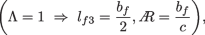
Symmetric airfoil of airship’s fin \(\left( \Rightarrow l_{f1}=l_{f2}=l_h+\dfrac{c}{4}\right)\),
-
4
No taper ratio
-
5
No dihedral angle \((\Gamma =0^\circ )\).
-
6
low speed \(\left( M_{no}<0.3\right)\),
-
7
Airship length is between two and three meters \((2m\le l\le 3m)\),
-
8
Airship’s fin is NACA-0006 \(\left( (t/c)_{\max}=0.06\right)\) with chord \(c=0.15l\) and span \(b_f=2.1b\) and the location of airship fin leading edge is \(l_h=0.79l\), where b is the airship minor axis.

Genetic algorithm optimization technique is used to solve this problem under some constraints to get the regular shape of the airship as shown in Fig. 8, which are
-
1
Rear major axis is greater than front major axis \(\left( a_2>a_1\right)\),
-
2
Front major axis is greater than minor axis \(\left( a_1>b\right)\) and

Regular Airship Shape
The optimization problem is to maximize the following cost function:
This cost function is constructed to reduce the effect of wind load \(\left( f_{y,a}, N_a\right)\) and drag force \(\left( f_{x,a}\right)\), to improve energy consummation efficiency, and to increase lift force \(\left( f_{z,a}\right)\) and pitching moment \(\left( M_a\right)\), to increase weight capacity and endurance range in case of engine failure. Table 1 shows the sign change in aerodynamic forces and moments according to the sign change in angle of attack \(\alpha\) and side-slip angle \(\beta\) with the same magnitude. If \(\alpha\) has a fixed positive or negative value and the sign of \(\beta\) changes with the same magnitude, the sign of \(f_{y,a}\) and \(N_{a}\) changes also with the same magnitude. Same conclusion is valid for \(F_{z,a}\) and \(M_a\) if \(\beta\) is fixed. So, the operating domain can be reduced to a quarter as the value of the cost function J depends on the absolute values of the aerodynamic forces and moments. The aerodynamic forces and moments have the same magnitude for a fixed absolute values of angle of attack and side-slip angle. This is due to the nature of the airship shape as it has two planes of symmetry.
The airship shape can be developed by various ways. In this case, three configurations are used to build airship shape,
-
1
NPL shape suggested by the National Physics Laboratory [32]: NPL shape can be considered as an intersection of two ellipses with different major axes and same minor axes. The equations of shape construction are clarified in Fig. 9.
-
2
GNVR shape developed by National Aerospace Laboratories [33]: GNVR shape consists of three parts: semi-ellipse, sector of a circle and sector of parabola. The equations of shape construction are clarified in Fig. 10.
-
3
Wang shape [34]: Wang shape is developed by a parametric equation clarified in Fig. 11.

NPL Shape

GNVR Shape

Wang Shape
3 Results
Genetic algorithm optimization solutions are carried out using MATLAB toolbox with population size equal to 50 and the number of generations equal to 50 of NPL, GNVR and Wang shapes at each corresponding angle of attack \((\alpha )\) and side-slip angle \((\beta )\) are presented as
-
1.
NPL optimal solutions: NPL shape is constructed by two parameters, the optimal solution of “\(a_N\)” parameter at every \(\alpha\) and \(\beta\) is shown in Fig. 12 and “\(b_N\)” parameter in Fig. 13. The value of the cost function at every possibility is presented in Fig. 14. The solution results show that the optimal solutions of “\(a_N\)” and “\(b_N\)” have the same behavior for all values of \(\alpha\) and \(\beta\). As shown, “\(a_N\)” starts with extreme maximum value for all values of \(\alpha\), then has a step drop, and then increases as \(\beta\) increases. Also, “\(b_N\)” begins with extreme minimum value for all values of \(\alpha\) then increases as \(\beta\) increases. And the cost function J decreases as \(\alpha\) increases for all values of \(\beta .\)
-
2.
GNVR optimal solutions: Figure 15 shows the optimal solution of “\(d_G\)”, the single variable of GNVR shap, at each \(\alpha\) and \(\beta\). The value of cost function is shown in Fig. 16. The solution results show that the optimal solutions of “\(d_G\)” are approximately constant for all values of \(\alpha\) and \(\beta\) and the cost function J increases as \(\beta\) increases for all values of \(\alpha .\)
-
3.
Wang optimal solutions: Wang shape is built by a parametric equation. Figures 17, 18, 19, 20 and 21 show the optimal solution of “\(a_W\)”, “\(b_W\)”, “\(c_W\)”, “\(d_W\)” and “\(l_W\)” at each \(\alpha\) and \(\beta\), respectively. The value of the cost function is presented in Fig. 22. The solution results show that the optimal solutions of “\(a_W\)” and “\(b_W\)” have the same pattern for all values of \(\alpha\) and \(\beta\). As shown, their values decrease as \(\alpha\) increases for all values of \(\beta\). Also, “\(c_W\)” and “\(d_W\)” have the same behavior for all values of \(\alpha\) and \(\beta\). “\(c_W\)” and “\(d_W\)” optimal values are approximately constant except for \(10^\circ \le \alpha \le 20^\circ\) and \(0^\circ \le \beta \le 10^\circ\) where the values have rapid changes. In addition, “\(l_W\)” optimal values are approximately constant except for the upper values of \(\alpha\) and \(\beta\). And the cost function J decreases as \(\alpha\) increases for all values of \(\beta .\)

NPL “\(a_N\)” parameter

NPL “\(b_N\)” parameter

Cost function values of NPL shape

GNVR “\(d_G\)” parameter

Cost function values of GNVR shape

Wang “\(a_W\)” parameter

Wang “\(b_W\)” parameter

Wang “\(c_W\)” parameter

Wang “\(d_W\)” parameter

Wang “\(l_W\)” parameter

Cost function values of wang shape
4 Discussion
The optimized solution is performed in two steps. First one is to choose the shape type which has the best performance for various values of \(\alpha\) and \(\beta\). Figure 23 shows the values of the cost functions of the three types, and the difference between these cost functions is shown in Fig. 24. Figure 24 visualizes the difference sign regardless the magnitude, since the yellow color indicates that the difference is positive and negative otherwise. It is clear that GNVR and NPL shapes are better than Wang shape. In addition, the statistics in Table 2 clarify that there is no major difference between these two types. However, Fig. 24 shows that GNVR is better at high side-slip angle \(\left( \beta >10^\circ \right)\). So, GNVR shape is the optimized solution in this study. Reddy Desham and Rajkumar S. Pant [35] CFD work shows that GNVR has the smallest volumetric drag coefficient among the other shapes NPL and Wang in a certain case, which give us an intuition to the solution.
The second step is to find the best GNVR shape parameter which fits the optimal solutions at every \(\alpha\) and \(\beta\). The optimized parameter can be determined using a weighted function for averaging as follows:

Cost Function Values of NPL, GNVR and Wang Shapes

Cost Function Difference between NPL, GNVR and Wang Shapes
Different optimal values of the parameter “\(d_G\)” corresponding to different weights are shown in Table 3. So, it is clear that there is no major difference of the values of the parameter “\(d_G\)” for different weights and this leads to choosing the optimal parameter as \(d_{G,opt.}=0.655748\) and Fig. 25 shows a diagram of the optimized airship.

Schematic diagram of optimized airship
5 Conclusion
This article presents a further analytical development of the semi-empirical aerodynamic model in Eq. 3 of airship to consider the effect of side wind in Eq. 4 depending on the symmetrical shape of the airship. This model depends only on airship main geometric parameters. The shape optimization problem is formulated by NPL, GNVR and Wang shapes to choose the one which achieves the best performance index, minimizes drag and wind load and maximizes lift and pitching moment, using the genetic algorithm optimization technique. GNVR shape exceeded their counterparts and consequently was adopted.
Availability of data and materials
The datasets used and/or analyzed during the current study are available from the corresponding author on reasonable request.
Abbreviations
- UAVs:
-
Unmanned aerial vehicles
- VTOL:
-
Vertical take off and landing
- C.V.:
-
Center of volume
- \(a\) :
-
Mean of the major axes of Airship, \(\dfrac{a_1+a_2}{2}\), \({m}\)
- \(a_N,b_N\) :
-
NPL shape parameters
- \(a_W,b_W,c_W,d_W,l_W\) :
-
Wang shape parameters
- \(a_s\) :
-
Sound speed, \(340 {m}\)/\({\text {s}}^3\)
- \(a_1,a_2\) :
-
Hull front and rare major axes, respectively, \({m}\)
- \(b\) :
-
Minor axis of airship, \({m}\)
- \(b_f,c\) :
-
Fin span and chord, respectively, \({m}\)
- \(C_{Dcf},C_{Dch}\) :
-
Fin and hull cross-flow drag coefficients, respectively
- \(C_{Df0},C_{Dh0}\) :
-
Fin and hull drag coefficients, respectively
- \(C_L,C_M,C_N\) :
-
Coefficients of aerodynamic moments \(L_{s}, M_{q}, N_{r}\), respectively, \(m^3\)
- \(C_{L,\alpha },C_{M,\alpha }\) :
-
Coefficients of aerodynamic moments \(L_{s,\alpha }, M_{q,\alpha }\), respectively, \({m}^3\)
- \(C_{L,\beta },C_{N,\beta }\) :
-
Coefficients of aerodynamic moments \(L_{s,\beta }, N_{r,\beta }\), respectively, \({m}^3\)
- \(C_X,C_Y,C_Z\) :
-
Coefficients of aerodynamic forces \(F_{s}, F_{q}, F_{r}\), respectively, \(m^2\)
- \(C_{X,\alpha },C_{Z,\alpha }\) :
-
Coefficients of aerodynamic forces \(F_{s,\alpha }, F_{r,\alpha }\), respectively, \({m}^2\)
- \(C_{X,\beta },C_{Y,\beta }\) :
-
Coefficients of aerodynamic forces \(F_{s,\beta }, F_{q,\beta }\), respectively, \({m}^2\)
- \(\left. \begin{array}{l} C_{L1}\\ C_{M1},C_{M2},C_{M3},C_{M4}\\ C_{N1},C_{N2},C_{N3},C_{N4} \end{array} \right\}\) :
-
Moments aerodynamic constants, \({m}^3\)
- \(\left. \begin{array}{l} C_{X1},C_{X2}\\ C_{Y1},C_{Y2},C_{Y3},C_{Y4}\\ C_{Z1},C_{Z2},C_{Z3},C_{Z4} \end{array} \right\}\) :
-
Forces aerodynamic constants, \({m}^2\)
- \(C_{d_{\min }}\) :
-
Fin minimum drag coefficient
- \(C_f\) :
-
Fin skin friction coefficient
- \(d_G\) :
-
GNVR shape parameter
- \(F_{s},F_{q},F_{r}\) :
-
Aerodynamic forces in \({s},\,{q}\) and \({r}\) directions, respectively, \({N}\)
- \(F_{s,\alpha }, F_{r,\alpha }\) :
-
Aerodynamic forces in \({s}\) and \({r}\) directions, respectively, due to the effect of \(V_{t,\alpha }\), \({N}\)
- \(F_{s,\beta }, F_{q,\beta }\) :
-
Aerodynamic forces in \({s}\) and \({q}\) directions, respectively, due to the effect of \(V_{t,\beta }\), \({N}\)
- \(F_{x,a},F_{y,a},F_{z,a}\) :
-
Aerodynamic forces in \({x}\), \({y}\) and \({z}\) directions, respectively, \({N}\)
- \(I_1,I_3,J_1,J_2\) :
-
Hull geometric integrals
- \(k_1,k_2\) :
-
Axial and lateral apparent-mass coefficients, respectively
- \(L_a, M_a, N_a\) :
-
Aerodynamic moments about \({x},\,{y}\) and \({z}\) axes, respectively, \({N}.{m}\)
- \(L_s, M_q, N_r\) :
-
Aerodynamic moments about \({s},\,{q}\) and \({r}\) axes, respectively, \({N}.{m}\)
- \(L_{s,\alpha }, M_{q,\alpha }\) :
-
Aerodynamic moments about \({s}\) and \({q}\) axes, respectively, due to the effect of \(V_{t,\alpha }\), \({N}.{m}\)
- \(L_{s,\beta }, N_{r,\beta }\) :
-
Aerodynamic moments about \({s}\) and \({r}\) axes, respectively, due to the effect of \(V_{t,\beta }\), \({N}.{m}\)
- l :
-
Hull length, \({m}\)
- \(l_{f1}\) :
-
\({x}\)-distance from nose to aerodynamic center of fins, \({m}\)
- \(l_{f2}\) :
-
\({x}\)-distance from nose to geometric center of fins, \({m}\)
- \(l_{f3}\) :
-
\({y}, \, {z}\)-distance from origin to aerodynamic center of fins, \({m}\)
- \(l_h\) :
-
Distance between hull nose and leading edge of airship fin, \({m}\)
- \(M_{no}\) :
-
Mach number, \(\dfrac{V_t}{a_s}\)
- \({\text{Re}}_{f}\) :
-
Reynolds number with maximum fin span reference length, \(\dfrac{\rho _{\infty } V_t\left( x_2-x_1\right) }{\mu _{\infty }}\)
- \({\text{Re}}_{l_h}\) :
-
Reynolds number with \(l_h\) reference length, \(\dfrac{\rho _{\infty } V_tl_h}{\mu _{\infty }}\)
- \(S_f\) :
-
Fin reference area, \({m}^2\)
- \(S_{fh}\) :
-
Intersection area between hull and Fin, \({m}^2\)
- \(S_h\) :
-
Hull reference area, \(V^{2/3}\), \({m}^2\)
- \(S_{wet}\) :
-
Fin wetted area, \({m}^2\)
- \({sqr}\) :
-
Aerodynamic frame of reference
- \(\left( t/c\right) _{\max}\) :
-
Maximum thickness to chord ratio of fin
- \({u},\,{v}, \,{w}\) :
-
Airship linear velocities in \({x},\,{y}\) and \({z}\) directions, respectively, \({m}\)/\({\text {s}}^3\)
- \({V}\) :
-
Airship volume, \({m}^3\)
- \(V_t\) :
-
Airship absolute velocity, \(\sqrt{u^2+v^2+w^2}\), \({m}\)/\({\text {s}}^3\)
- \(V_{t,\alpha }\) :
-
Airship absolute velocity component due to \(\alpha\), \(\cos (\beta )V_t\), \({m}\)/\({\text {s}}^3\)
- \(V_{t,\beta }\) :
-
Airship absolute velocity component due to \(\beta\), \(\cos (\alpha )V_t\), \({m}\)/\({\text {s}}^3\)
- \(Xyz\) :
-
Airship frame of reference
- \(x_n\) :
-
Distance between hull nose and airship C.V., \({m}\)
- \(x_1\) :
-
Distance between hull nose and front point of \(S_{fh}\) across negative \(x\)-axis, \({m}\)
- \(x_2\) :
-
Distance between hull nose and rare point of \(S_{fh}\) across negative \(x\)-axis, \({m}\)
- \(\alpha\) :
-
Angle of attack, \({radian}\)
- \(\beta\) :
-
Side-slip angle, \({radian}\)
- \(\Gamma\) :
-
Dihedral angle, \({radian}\)
- \(\delta _{eL},\delta _{eR}\) :
-
Left and right horizontal stabilizer deflections, respectively, \({radian}\)
- \(\delta _{rT},\delta _{rB}\) :
-
Top and bottom vertical stabilizer deflections, respectively, \({radian}\)
- \(\eta _f\) :
-
Fin-efficiency factor accounting for the effect of the hull on the fins
- \(\eta _k\) :
-
Hull-efficiency factor accounting for the effect of the fins on the hull
- \(\Lambda\) :
-
Taper ratio
- \(\mu _{\infty }\) :
-
Dynamic viscosity of air, \(1.785\times 10^{-5}\,{\text {kg/m/s}}\)
- \(\rho\) :
-
Air density with standard value, \(\rho _\infty =1.225\,{\text {kg/m}}^3\)
-
 :
: -
Aspect ratio
- \(\left( \dfrac{\partial C_l}{\partial \alpha }\right) _f\) :
-
Derivative of fin lift coefficient with respect to the angle of attack at zero incidence
- \(\left( \dfrac{\partial C_l}{\partial \delta }\right) _f\) :
-
Derivative of fin lift coefficient with respect to the flap deflection angle
 :
:References
Manikandan M, Pant RS (2021) Research and advancements in hybrid airships—a review. Prog Aerospace Sci 127:100741
Colozza A, Dolce J (2003) Initial feasibility assessment of a high altitude long endurance airship. NASA/CR 212724
Anderson JD, Bowden ML (2021) Introduction to flight, 9th edn. McGraw-Hill Education, New York
d’Oliveira FA, Melo FCLd, Devezas TC (2016) High-altitude platforms–present situation and technology trends. J Aerospace Technol Manag 8, 249–262
Frezza L, Marzioli P, Santoni F, Piergentili F (2021) Vhf omnidirectional range (VOR) experimental positioning for stratospheric vehicles. Aerospace 8(9):263
Marzioli P, Di Palo L, Garofalo R, Collettini L, Picci N, Bedetti E, Celesti P, Misercola L, Di Nunzio C, Pancalli MG et al (2022) Stratospheric balloon tracking system design through software defined radio applications: Strains experiment. Acta Astronaut 193:744–755
Eissing J, Eissing CS, Fink E, Zobel M, Antrack F (2023) Airship sling-load operations: a model flight-test approach. In: Lighter than air systems, pp 37–51
Adorni E, Rozhok A, Revetria R (2023) Application of airships in the surveillance field. In: International multiconference of engineers and computer scientists. Springer, pp 40–52
Burns R (2001) Advanced control engineering. Elsevier, New York
Arqub OA, Abo-Hammour Z (2014) Numerical solution of systems of second-order boundary value problems using continuous genetic algorithm. Inf Sci 279:396–415
Abo-Hammour Z, Abu Arqub O, Momani S, Shawagfeh N (2014) Optimization solution of Troesch’s and Bratu’s problems of ordinary type using novel continuous genetic algorithm. Discrete Dyn Nat Soc 2014
Munk MM (1979) The aerodynamic forces on airship hulls. Class Aerodyn Theory 111
Allen HJ, Perkins EW (1951) Characteristics of flow over inclined bodies of revolution. Research Memorandum A50L07, National Advisory Committee for Aeronautics
Hopkins EJ (1951) A semi-empirical method for calculating the pitching moment of bodies of revolution at low Mach numbers
Jones S, DeLaurier J (1983) Aerodynamic estimation techniques for aerostats and airships. J Aircr 20(2):120–126
Cui Y, Zhou J, Miao J, Wang F, Yang Y (2020) The yaw stability analysis for stratospheric airships in float situation. Adv Space Res 65(5):1375–1382
Li Y, Nahon M, Sharf I (2011) Airship dynamics modeling: a literature review. Prog Aerospace Sci 47(3):217–239
Li Y, Nahon M (2007) Modeling and simulation of airship dynamics. J Guid Control Dyn 30(6):1691–1700
Williams JE, Vukelich SR (1979) The USAF stability and control digital Datcom. Volume I. users manual. Technical report, McDonnell Douglas Astronautics Co St Louis Mo
Lutz T, Wagner S (1998) Drag reduction and shape optimization of airship bodies. J Aircr 35(3):345–351
Nejati V, Matsuuchi K (2003) Aerodynamics design and genetic algorithms for optimization of airship bodies. JSME Int J Ser B Fluids Therm Eng Jpn Soc Mech Eng 46(4):610–617
Wang X-l, Shan X-x (2006) Shape optimization of stratosphere airship. J Aircraft 43(1):283–286
Ram CV, Pant RS (2010) Multidisciplinary shape optimization of aerostat envelopes. J Aircraft 47(3):1073–1076
Hassanzadeh RA, Shariatmadari S, Chegeni A, Ghazanfari SA, Nakisa M (2014) Survey on the indirect methods of potential flow used for the optimization of airships profile. In: Applied mechanics and materials. Trans Tech Publ, vol 554, pp 717–723
Ma D, Li G, Yang M, Wang S, Zhang L (2019) Shape optimization and experimental research of near space airship. Proc Inst Mech Eng Part G J Aerospace Eng 233(10):3589–3602
Li G, Wang J (2020) Shape optimization of near-space airships considering the effect of the propeller. J Aerospace Eng 33(5)
Hoerner SF (1965) Fluid dynamic drag, published by the author. Midland Park, NJ, 16–35
Sadraey M (2009) Aircraft performance: analysis. VDM Publishing, Saarbröcken
Robinson M (1977) Cross-flow characteristics on a cylindrical body at incidence in subsonic flow. In: Institution of Engineers, Australian Hydraulics and Fluid Mechanics Conference, 6 th, Adelaide, Australia
Wardlaw A (1979) High-angle-of-attack missile afrodynamics. Furnished to DTIC contained
Munk MM (1936) Aerodynamics of airships: aerodynamic theory. Springer, Berlin, pp 32–48
Kale S, Joshi P, Pant R (2005) A generic methodology for determination of drag coefficient of an aerostat envelope using CFD. In: AIAA 5th ATIO and16th Lighter-Than-Air Sys Tech. and Balloon Systems Conferences
Narayana C, Srilatha K (2000) Analysis of aerostat configurations by panel methods. BLISS Project Document CF 10
Alam MI, Subhani S, Pant RS (2014) Multidisciplinary shape optimization of stratospheric airships. In: International conference on theoretical, applied, computational and experimental mechanics (ICTACEM-2014)
Reddy MD, Pant RS (2018) CFD analysis of axisymmetric bodies of revolution using openfoam. In: 2018 applied aerodynamics conference, p 3334
Acknowledgements
The authors would like to thank all the contributors who directly or indirectly helped us in the preparation of this article.
Funding
The authors did not receive support from any organization for the submitted work.
Author information
Authors and Affiliations
Contributions
GM conceived the study. MA structured the content, wrote, and organized the article. ML edited and revised the full article. GM revised the manuscript. All authors read and approved the final manuscript.
Corresponding author
Ethics declarations
Ethics approval and consent to participate
Not applicable.
Consent for publication
Not applicable.
Competing interests
The authors declare that they have no competing interests.
Additional information
Publisher's Note
Springer Nature remains neutral with regard to jurisdictional claims in published maps and institutional affiliations.
Rights and permissions
Open Access This article is licensed under a Creative Commons Attribution 4.0 International License, which permits use, sharing, adaptation, distribution and reproduction in any medium or format, as long as you give appropriate credit to the original author(s) and the source, provide a link to the Creative Commons licence, and indicate if changes were made. The images or other third party material in this article are included in the article's Creative Commons licence, unless indicated otherwise in a credit line to the material. If material is not included in the article's Creative Commons licence and your intended use is not permitted by statutory regulation or exceeds the permitted use, you will need to obtain permission directly from the copyright holder. To view a copy of this licence, visit http://creativecommons.org/licenses/by/4.0/.
About this article

Cite this article
Atyya, M., ElBayoumi, G.M. & Lotfy, M. Optimal shape design of an airship based on geometrical aerodynamic parameters. Beni-Suef Univ J Basic Appl Sci 12, 25 (2023). https://doi.org/10.1186/s43088-023-00352-1
Received:
Accepted:
Published:
DOI: https://doi.org/10.1186/s43088-023-00352-1