
Abstract
Short-term constituents of the secular variation, at inter-decadal (20–30 years) and sub-centennial (60–90 years) time scales, present in observatory data and main field models, are also found in the radial field evolution at core surface. The paper is focused on the sub-centennial constituent in the gufm1 model. Time–Longitude (t–λ) plots, covering the 400 years time span of the model, at various latitudes between 70°N and 70°S, show a clear westward movement of the sub-centennial constituent field features in the 20°N–20°S latitude band. The sub-centennial constituent at latitudes larger than 50°N/S stands in fact for the fine structure of high-latitude flux lobes. Since 1900 this fine structure shows a westward displacement. Time–Latitude (t–φ) plots indicate also northward and southward components of the movement. The traveling speeds of the sub-centennial constituent field are derived, on one hand, empirically based on Time–Longitude and Time–Latitude plots, and on the other, mathematically by means of the Radon transform method. Important results of this paper are related to characterization of the evolution of the radial field at core surface at sub-centennial time scales, namely (1) evidencing two types of azimuthal flow, equatorial and high latitude ones, responsible for the observed westward drift of the surface field, and (2) quantitative information on meridional displacements of the core surface magnetic flux patches.

Introduction
The main geomagnetic field and its secular variation (SV) are, together with geodynamo modeling, a source of information on possible movements of the conductive fluid of the outer core that lead to the generation of the field. A broad spectrum of aspects regarding modeling of the core flow from geomagnetic secular variation has recently been reviewed by Holme (2015), including a history of theories regarding the well-known westward drift of the field, from Haley (1692) to Bullard et al. (1950), and to Yukutake and Tachinaka (1969) and Yukutake (1979). Recently, Yukutake and Shimizu (2015, 2016) have decomposed the geomagnetic gufm1 model of Jackson et al. (2000) into drifting and standing fields, the former being dominated by sectorial terms of the spherical harmonic coefficients.
The long time span models of the main geomagnetic field produced in the last two decades based on geomagnetic data, namely gufm1 (Jackson et al. 2000), IGRF-12 (Thébault et al. 2015), CM4 (Sabaka et al. 2004), COV-OBS (Gillet et al. 2013), allow to compute the core-mantle boundary field evolution, from which the flow at the top of the core can be obtained.
Recently, Finlay and Jackson (2003), Finlay (2005) and Jackson and Finlay (2007), investigating the nonaxisymmetric field at the core surface using gufm1, have been able to infer the existence of westward moving field features. After removing from the radial field at the core surface the time-averaged axisymmetric component, they high-pass filtered the field with a cutoff period of 400 years. Alternate sign magnetic flux patches in the equatorial band highlighted by that procedure show a westward motion of about 17 km/year. This movement was explained by three possible mechanisms (1) an equatorial jet, (2) a MAC (Magnetic, Archimedes, Coriolis) wave, or (3) a combination between a jet and a MAC wave. Robust westward drift and time-dependence of low-latitude secular variation similar to that observed over the past 400 years are achieved in a coupled Earth dynamo model for the last 3000 years filtered to spherical harmonic degree and order 8 (Aubert et al. 2013), implying the existence of a giant, westward drifting, sheet-like gyre reaching closer to the outer core surface in the Atlantic Hemisphere (between 90°W and 90°E), in agreement with core flow inversions of secular variation data (Pais and Jault 2008). Pais et al. (2015) identify core circulation modes that explain 95% of the secular variation induced by the total flows and can alter the eccentric gyre. Lhuillier et al. (2011) discuss the SV timescale in observations and numerical dynamo models from the perspective of the power spectral density that characterizes each degree of the spherical harmonic expansion that describes data (CHAOS, gufm1) or numerical geodynamo models.
Terra-Nova et al. (2015) using the archeomagnetic field model CALS3k.4b of Korte and Constable (2011), for the interval 990 B.C.–1990 A.D., showed the presence of reversed flux patches at the core surface that are moving mostly westward with an average rate of 0.10°/year. Also, in both hemispheres most of the reversed flux patches migrate toward poles. Recently, Metman et al. (2017) showed that the reversed flux patches are responsible for two-thirds of the dipole decay over the twentieth century the rest of the decay being caused by the evolution of the normal field.
Secular variation studies developed by Demetrescu and Dobrica (2005, 2014) and Dobrica et al. (2013) on long time series (100–150 years) of observatory data showed that the surface field and its SV are constituted of oscillations at time scales of ~ 11, ~ 22 and ~ 80 years, which are superimposed on a (quasi)linear trend denoted steady variation. The “decadal,” 11-year oscillation is considered as solar-cycle-related, contaminating the observatory annual means, while the ~ 22, ~ 80 year, and steady constituents are of internal origin. We are aware that a decadal signal could also have a partial internal origin, if only the induced response to external variations, the amplitude of which is assessed to ~ 1/3 of the inducing one (Price 1967; Xu et al. 2015), was considered. Also, decadal and shorter signals originating in the Earth’s core have been recently studied (Gillet et al. 2010; Silva et al. 2012; Holme and de Viron 2013; Cox et al. 2016); however, additional effort is needed to decide on the origin and degree of overlapping. As the gufm1 model is based mainly on observatory data for the period 1840–1990, the presence of the oscillations at time scales of ~ 11, ~ 22 (actually 22–30) and ~ 80 (actually 60–90) years in model data is expected too. Stefan (2011) extended these studies in case of H, D and Z components of the main field and of SV at Earth surface using three of the four main field models mentioned above, namely gufm1, IGRF (IGRF-11, Finlay et al. 2010b), CM4, inferring a westward motion of the two internal, oscillatory constituents field features. These constituents show, in the three models, similar spatial and temporal evolution for the overlapping periods. In what follows we shall call “inter-decadal” and “sub-centennial” the two oscillatory constituents at timescales of 20–30 and 60–90 years, respectively. The amplitude of the sub-centennial constituent, of several hundred nT in H and Z, is several times larger than the inter-decadal one. In terms of the secular variation, the contribution of the solar-cycle-related and of the two internal constituents is similar, hence the need of eliminating the decadal one in SV analyses. When looking at 400 years of data [see, e.g., a discussion based on historical declination data from several locations in Western Europe and on gufm1 time series in Demetrescu and Dobrica (2014)], an evolution of the field emerges characterized by a slow variation at a timescale that seems larger than 400 years. We shall call this constituent, that bears the largest part of the field, “inter-centennial.” We stress the fact that due to linear extrapolation of the magnetic moment prior to 1840 in gufm1, for which a 15 nT/year decay rate was assumed, the inter-centennial constituent might have a different morphology when other dipole decay rate would be considered (e.g., ~ 2 nT/year, Gubbins et al. 2006). The two oscillations mentioned above are expected to superimpose on the inter-centennial constituent, no matter what morphology of the latter is.
It is well known that in long-term main field models such as gufm1 the field at the core surface is determined by downward continuation of the surface field through the source-free mantle (e.g., Parker 1994). Thus, the surface field constituents highlighted in previous studies by Demetrescu and Dobrica (2005, 2014) and Dobrica et al. (2013) are expected to be found in the field at the core surface as well. In this paper we focus on the detailed structure of the radial field flux patches given by the sub-centennial constituent in gufm1 as we analyze its morphology, spatial–temporal characteristics and traveling speeds at core surface. "Data and method" are presented in second section of the paper along with time-averaged energy maps of the field and of its three constituents. In "Results and discussion" section we discuss the results concerning the sub-centennial constituent in terms of geographical distribution maps, Time–Longitude plots, and traveling speeds. Movements in the north–south direction that were mentioned in literature (Finlay et al. 2016a) are quantitatively investigated through Time–Latitude plots and subsequent speed information. Fourth section is reserved for "Conclusions".
Data and method
The gufm1 main geomagnetic field model, covering the time span 1590–1990, was used to obtain time series of the radial component at the core surface (core-mantle boundary—CMB), Zc, in a 2.5° × 2.5° latitude/longitude grid, between 70°S and 70°N. The code and coefficients of the model are available online at http://www.epm.geophys.ethz.ch/~cfinlay/.
To separate constituents at decadal, inter-decadal, sub-centennial, and inter-centennial time scales, the radial field time series, for each grid point, were treated by means of a filtering method that uses successive running averages with windows of 11, 22 and ~ 78-years (Demetrescu and Dobrica, 2005, 2014). For a detailed discussion regarding the mathematical formalism of the running averages filter and its effect on oscillatory constituents see Appendix of Demetrescu and Dobrica (2014). Successively smoothed times series result, denoted Zc11, Zc22, and, respectively, Zc78, and differences between them give what we call inter-decadal (Zc22–Zc11) and sub-centennial (Zc22–Zc78) constituents of the radial field at the core surface. Zc78 is the inter-centennial constituent, and the difference between data and Zc11 is the decadal constituent. We note here that smoothing the time series by an ~ 80-year running window results in inter-centennial and sub-centennial time series that are about 40-years shorter at each end than the unfiltered one (i.e., they span the time interval 1630–1950). Other options would have been to use Hodrick–Prescott (1997) analysis, to separate a cyclic component at the decadal time scale from a trend, and then successive high-pass Butterworth filtering of the trend with 22 and 78 years cutoffs. For a discussion regarding advantages and/or disadvantages of the filtering methods used to decompose the main field and its SV in case of radial field at the core surface, as well as regarding the sub-centennial signal in gufm1 coefficients, see Appendixes 1 and 2, respectively. It can be demonstrated (Demetrescu and Dobrica 2014, Appendix) that the information regarding the actual periodicities would not be lost, no matter what value is adopted for the windows length or cutoffs, unless it is a multiple of the true period in data. In this paper we preferred the running averages also because they can account well for slightly nonstationary signals. We show as an example, in Fig. 1, several superposed time series of the radial field sub-centennial constituent and of its time derivative at the core-mantle boundary (CMB). These were obtained using running averages, for the location of nine European observatories. The latter is a geographically localized network of points, supposed to show similar response to core surface sources, response otherwise location dependent in case of a sparser network of points. It can be seen that there is not a clear (quasi)periodicity of the radial sub-centennial constituent of the field. Rather, oscillations of the field components show a changing morphology in time, including a certain irregularity in the succession of peaks.

Time series of the sub-centennial constituent (top) and their time derivative (bottom) of the core surface radial field for the location of nine European observatories (IAGA codes are associated with various line colors)
Decomposition of the core radial field into its three constituents in terms of energy maps, obtained by squaring and averaging the field values over the time span 1630–1950, is presented in Additional file 1: Fig. S1. It can be seen that the energy of the inter-centennial constituent is two orders of magnitude larger than of the sub-centennial constituent, and four orders of magnitude larger than of the inter-decadal constituent. This makes it responsible for most of the SV, with maximum in the South Atlantic and a weaker one at equatorial Africa; lower energy (1/3 and lower) characterizes areas such as north of South America, North America, Indian Ocean and Asia. Two areas are characterized by maximum values of the energy of the sub-centennial constituent, namely northern South America–eastern North America in the Northern Hemisphere, and southern Africa–southern Indian Ocean in the Southern Hemisphere. The energy in case of the inter-decadal constituent, two orders of magnitude less than the energy of the sub-centennial constituent, affects about the same areas as the sub-centennial one.
Another form to measure the temporal variability of the geomagnetic field, introduced by Constable et al. (2016), is to compute the standard deviation over a certain time interval; the result in case of gufm1 (see their Fig. 1) shows, as expected, a similar distribution of active areas. Their study regarding the last 10,000 years, based on two new global time-varying paleomagnetic field models, emphasize that the Southern Hemisphere field has been more active than the Northern Hemisphere one. Our maps identify two sources that might have been responsible for the variability in the Southern Hemisphere in the last 10,000 years: the inter-centennial variation, located ‘now’ (gufm1, 1590–1990) at the southern tip of South America, and the sub-centennial constituent, active in southern Africa—southern Indian Ocean. We note that only the former could be seen by the paleomagnetic field models investigated by Constable et al. (2016); the latter falls under the sensitivity of models input data due to its lower amplitude range.
In the rest of the paper we will deal only with the sub-centennial constituent as we consider that it is responsible to a large extent for the fine structure of the main field and its SV. We leave a detailed analysis of the inter-centennial constituent for another publication.
Time–Longitude (t–λ) and Time–Latitude (t–φ) plots (Hovmöller 1949) for various latitudes, respectively, longitudes, with a spatial step of 2.5° and a temporal one of 2.5 years were constructed in order to investigate the spatial and temporal characteristics of the sub-centennial constituent of the radial field at the core surface. Such plots allow only a visual, time-consuming interpretation to get information on the geographical distribution and the traveling speeds of those characteristics. In order to infer a global quantitative information, a Radon transform (Deans 2000), that was used in previous geomagnetic field studies by Finlay and Jackson (2003), Finlay (2005), Jackson and Finlay (2007), was applied. Following Finlay (2005), the Radon transform of a two dimensional image is the projection of that image in the direction normal to the line defined by a certain angle. The two dimensional image in our case is represented by (t–λ) and (t–φ) plots. The angle that defines the projection line varies between − 90° and 90° and for every projection a curve results, with the largest peak indicating the dominant speed highlighted on the analyzed Time–Longitude/Latitude plot. The projection values are stored into an array. The resulted array values, after applying the method to every Time–Longitude or Time–Latitude plot, are squared and summed along the time axis and then combined in a new array. This new array, latitude-azimuthal-speed (LAS)/longitude-meridional-speed (LMS), contains the energy of the image as a function of latitude/longitude and the traveling speeds—positive indicating eastward/northward movements, negative indicating westward/southward movements.
Finally, to localize areas characterized by important displacements and intensity variations of the magnetic flux patches of the radial component of the sub-centennial constituent, the mean energy of its secular variation for each point of the 2.5° × 2.5° grid was calculated by averaging the squared values of the SV for the 320 years time span (1630–1950) of the sub-centennial constituent.
We end this section by stressing that our way of looking at geomagnetic field and SV data, be they observed or main field model time series, is quite different from the current approach based on a separation of the field constituents according to various terms of the spherical harmonic expansion of the field. We decompose the field and its SV according to the well separated temporal windows already seen in geomagnetic data at inter-decadal (20–30 years), sub-centennial (60–90 years), and inter-centennial (≥ 400 years) timescales, probably caused by core flow evolutions with different intensities and geographical patterns at the corresponding timescales. Consequently, we find this kind of variability in every spherical harmonic coefficient, including the axial dipole one and going to the last coefficient of gufm1, of degree and order 14. However, besides the main period of 60–90 years, shorter ones are seen in some cases (see Appendix 2). Also, expected phase differences and certain amplitude degrading prior to 1840 affect the time evolution of the sub-centennial constituent. The amplitude degrading in coefficients before 1840 is a consequence of using historical data in deriving gufm1 (i.e., Gauss coefficients) before the observatory era. The coefficients alone cannot tell any story about the evolution of the field as, in predicting the field constituent using the spherical functions expansion, coefficients multiply by various functions of latitude and longitude to give location-dependent field values.
Results and discussion
Geographical distribution of the sub-centennial constituent at the top of the core
Maps at various times in the 320 years interval (1630–1950) of the sub-centennial constituent show positive and negative magnetic flux patches that migrate in space and time. In Additional file 2: Fig. S2 a movie showing the temporal evolution of the studied constituent of the core field is given. Alternating patches of opposite sign traveling westward are observed in the ± 30° latitude band. Besides, some of the magnetic flux patches are observed to behave in a more complex manner. For instance, the positive patch under the North of South America is decomposing in 1850 in two new patches, one migrating toward North, to the East coast of the North America, and one moving in southward direction, to the west coast of the South America. A similar situation is also observed under the Atlantic, where a positive and a negative flux are splitting in two. During the time interval 1640–1730 the positive flux patch under the Pacific is growing in intensity and is extending its spatial coverage.
Evolution of sub-centennial constituent flux patches
The evolution of sub-centennial flux patches at the core surface is discussed based on both Time–Longitude/Latitude plots and LAS/LMS power plots. The two approaches allow assessing traveling speeds of the sub-centennial constituent field features.
Time–Longitude and Time–Latitude plots
Time–Longitude plots, presented in Figs. 2 and 3 for selected latitudes, show three different regimes of temporal evolution, depending on latitude, namely: (1) alternating positive and negative strips indicating a westward motion of field features in the ± 20° latitude band in the Atlantic hemisphere (between 90°W and 90°E) during the entire time span of the model; (2) magnetic flux patches with indications of eastward movements in certain intervals of the model time span (e.g., 1800–1870), at high latitudes (60°–70°N, S); and (3) transitional behavior at low-mid latitudes (30°–40°N). The latter indicates the first two latitude bands have northern and, respectively, southern extensions (e.g., flux patches moving westward during the entire time span with the same speed as the equatorial ones, like the positive patch between 60 and 90°W at 1640, or, respectively, weak positive patches that get stronger at higher latitudes, seen in the first 150–200 years of gufm1 in the 40°N plot). Also, at low-mid latitudes a complex behavior characterizes the flux patches after 1800.

Time–Longitude plots of the core surface radial component of the sub-centennial constituent for selected middle-high latitudes. Movement direction is highlighted by straight line segments

Time–Longitude plots of the core surface radial component of the sub-centennial constituent for selected low-middle latitudes. Movement direction is highlighted by straight line segments
The pattern of the sub-centennial flux patches evolution described above characterizes at least two different systems, one in an equatorial band of ± 20°, and one at northern and southern latitudes larger than 50°. The former is directly comparable with results published by Finlay and Jackson (2003), Finlay (2005) and Jackson and Finlay (2007), as regards direction and speed of movements of core surface flux patches.
As regards the equatorial system, for instance, positive flux patches traveled westward about 70°–90° in a period of 270–320 years, corresponding to a traveling speed of about 0.26°–0.27°/year (16–17 km/year), while negative flux patches are characterized by displacements of 45 degrees over an interval of 200 years, meaning a moving speed of ~ 0.23°/year (~ 14 km/year). The dominant traveling speed of ~ 17 km/year is also observed at Northern Hemisphere mid latitudes (20°–40°). The moving speeds are increasing at higher latitudes (40°–60°N) ranging from about 20 km/year up to about 26 km/year. This is in line with the flow calculations of Gillet et al. (2015a) that show a westward planetary gyre along the equator and midlatitude eddies with westward flow in the Atlantic hemisphere. A less clear picture characterizes the Southern Hemisphere, perhaps as a result of poorer input data coverage of the model. The Pacific hemisphere (between 90°E and 90°W) is characterized by seemingly standing patches, over periods of about 100 years, of weaker, time variable intensity, with a (quasi)period of ~ 80 years.
The high-latitude systems in the two hemispheres describe oscillations about the inter-centennial constituent of the field that take place at core surface between the 50° and the 70° parallels, close to the tangent cylinder, approximately marked by the 70° parallel. The flux patches in Fig. 2 (50°–70°N) represent the fine structure of high-latitude lobes. It is interesting that Livermore et al. (2016) observe contemporary intense high-latitude secular variation related to the westward evolution of the two high-latitude flux lobes predicted by the CHAOS-6 model (Finlay et al. 2016b), and infer, based on the westward drift of flux patches, the presence of an accelerating jet at CMB around the tangent cylinder. Their flux patches, defined for the time interval 1999–2016, are present in our t–λ plots at 1950, at a position corresponding to the westward displacement since. The fine structure detected by the higher resolution CHAOS-6 corresponds to our flux patches determined as oscillations about the inter-centennial very slow time-variation.
The t–λ plots in Fig. 2 (50°–70°N) also show the presence of alternating westward and eastward movements of the high-latitude flux patches in certain time intervals, also remarked by Livermore et al. (2016). However, our interpretation of flux patches displacements in the 50°–70°N might be somewhat subjective (e.g., the eastward movement after ~ 1840) and should be confirmed by further studies. We note that Dumberry and Finlay (2007) found that both eastward and westward motions of magnetic field features at the CMB have occurred in the past 3000 years, captured by the archaeomagnetic field model CALS7K.2 of Korte and Constable (2005), motions related to displacements and distortions of the two high-latitude flux lobes.
Finally, we would like to stress that our t–λ plots include two types of information: (a) information on field flux patches direction and speed of movement which is, in the equatorial band, similar to that previously found by Finlay and Jackson (2003) for oscillations in a time window of 400 years, and (b) information on intensity variations of both axisymmetric and nonaxisymmetric parts of the field, as the sub-centennial constituent is present in all terms of the time-dependent spherical harmonic expansion that describes the geographical distribution and the time evolution of the core field.
The strong latitude dependence of the westward drift of the sub-centennial constituent (and of its time derivative) at the CMB gets weaker at the Earth’s surface due to the attenuation of this relatively short wavelength variation, but it still exists, at odds with Yukutake and Shimizu (2016) that state the westward drift of the secular variation at Earth’s surface is latitude independent.
Migration of the magnetic flux patches in the north–south direction is analyzed by means of Time–Latitude plots (Fig. 4). We marked the equator by a vertical line, to show that the analysis should consider separately the two hemispheres because of the quasi-geostrophic character of the geomagnetic field at the CMB (Amit and Olson 2004; Pais et al. 2015). In comparison with latitudinal movements, the meridional ones are less coherent. This shows that the east–west movement is dominant. Dominant traveling speeds of 25–58 km/year correspond to displacements toward north that are seen in the longitude band 60°–120°W. Under the Atlantic Ocean the magnetic flux patches have the tendency to move southward with about 20 km/year. Although the northward movement is not dominant under the Atlantic, it is characterized by speeds that reach 50 km/year. Negative and positive magnetic flux patches of the sub-centennial constituent move toward north with speeds of 45 km/year. The Pacific area is characterized by flux patches traveling both northward and southward. Their speeds vary from 17 km/year to about 50 km/year. Stationary patches are observed in this area too.

Time–Latitude plots of the core surface radial component of the sub-centennial constituent for selected longitudes. Vertical green line marks the equator. Movement direction is highlighted by straight line segments
A robust assessment on moving magnetic flux patches can be achieved by a Radon transform method applied to all Time–Longitude/Latitude plots, in the form of LAS and LMS power plots, this kind of analysis bringing information regarding the traveling speeds and the latitude/longitude band where the movements take place. The results are presented in the next section.
Traveling speeds
The LAS power plot (Fig. 5) shows a dominant peak in the equatorial band corresponding to a traveling speed of about 17 km/year. Lower energy peaks, at mid latitudes, indicate speeds of about 35–40 km/year in the Southern Hemisphere, respectively, 16 km/year in the Northern Hemisphere. Also, a weak movement of about 10 km/year toward east, north of the equator, is marked on the LAS power plot by a low energy peak at positive speeds. These results are similar to those obtained by Finlay and Jackson (2003) and Jackson and Finlay (2007) for wave-like nonaxisymmetric field features with a period within a window of 400 years.

Latitude-azimuthal-speed power plot of the core surface radial component of the sub-centennial constituent
Displacements in the north–south direction are analyzed based on the LMS power plots, separately for the Northern and Southern hemispheres (Fig. 6), as cross-equator flows are forbidden in the quasi-geostrophic system described by gufm1 or COV-OBS (Pais et al. 2015). A first look at the plots reveals the lower energy of the peaks as compared to the energy in the LAS plot of Fig. 5, probably due to less coherent structures that characterize the Time–Latitude plots of Fig. 4. The plots reveal both northward and southward movements of the sub-centennial flux patches. In the Northern Hemisphere equatorward flows are present along the longitude of 30°E and, with a much weaker energy, along the 60°W meridian, while poleward movements can be spotted along the 40°E, 100°E, and 80°W meridians. In the Southern Hemisphere a poleward displacement is seen in the 60°–90°W longitude band, and an equatorward one along the 60°W meridian. The rather large speeds, of about 40–50 km/year could arise due to less clear appearance of the flux patches on the Time–Latitude plots. In an attempt to explain the dipole field decay since 1840, Finlay et al. (2016a) invoke fluctuations of meridional flux advection present in two longitude bands, namely an equatorward flow around longitude 100°E and a poleward one around 90°W, as parts of a planetary gyre. Terra-Nova et al. (2015) and Metman et al. (2017) identify the role of reversed flux patches in diminishing the dipole field. The former investigate a time span from 990 BC to 1990 AD using the CALS3k.4b model of Korte and Constable (2011), which is constrained by gufm1 from 1840 onward, while the latter investigate the time span from 1840 to 2015 using gufm1, COV-OBS.x.1 (Gillet et al. 2015b), and CHAOS-6 (Finlay et al. 2016b). Future studies are necessary in order to fit in our results in such models. For the moment, we stress the fact that (1) the sub-centennial oscillation we study in this paper is only one of the constituents of the core field, (2) it is present in all Gauss coefficients of gufm1, g10 included, and (3) it is an oscillation about the inter-centennial variation and by no means the corresponding alternate sign patches in Figs. 5 and 6 can be assimilated to reversed flux patches of Terra-Nova et al. and Metman et al. (op. cit.).

Longitude-meridional-speed power plot of the core surface radial component of the sub-centennial constituent in case of Northern Hemisphere (top) and Southern Hemisphere (bottom)
Pais et al. (2015) compare core flows inferred from gufm1 and COV-OBS for the overlapping time interval of the two models and decompose the core flow based on Principal Component Analysis and Singular Value Decomposition to derive three main empirical circulation modes that add to the mean flow for 1840–2010 (170 years). It is interesting that in one of the three modes, namely Mode 2, highlighted by Pais et al. (2015), the regions close to the tangent cylinder and to the equator are correlated and oscillate with a period of 80–90 years. However, the sub-centennial oscillation that we discuss in the present paper, due to the way is derived, regards all field constituents.
Sub-centennial active regions
In order to highlight areas where important displacements of the magnetic flux patches and intensity variations have taken place during the 320 years time span (1630–1950) of the sub-centennial constituent of the radial field, we determined the time-averaged energy of its secular variation (Fig. 7); see also Additional file 1: Fig. S1, for the main field constituent. The secular variation-related activity of this constituent is concentrated in the Atlantic hemisphere, as it is generally the case with the observed surface secular variation (e.g., Finlay and Jackson 2003; Aubert et al. 2013). An active area under the north of South America that extends toward north up to the East coast of USA and Canada indicates important displacements and intensity variations in time that have taken place under this region. Active areas are also seen under the southern tip of the African continent and under the Indian Ocean, corroborating studies on rapid evolution of the surface geomagnetic field in that area (Mandea et al. 2007; Kotzé and Korte 2016). In terms of main field models, Whaler (1986) had already noticed fast and strong SV under the Indian Ocean and southern Africa, shown later also by GRIMM models (Lesur et al. 2008, 2010; Mandea et al. 2012). Under the Atlantic Ocean, Central and East Europe, Central and East Asia, and West coast of the African continent, especially Gulf of Guinea, less dominant changes, marked by lower energy areas, show up.

Geographical distribution of the time-averaged energy of the secular variation of the radial field of the sub-centennial constituent, at the CMB, during the time interval 1630–1950
Conclusion
Using a filtering approach that successively eliminates oscillatory behavior at certain timescales, present in the gufm1 radial field at core surface, we showed that a sub-centennial (timescale of 60–90 years) oscillation is responsible for the fine structure of the time evolution of the geomagnetic field at the core-mantle boundary. It is superimposed on a slowly varying constituent, at inter-centennial timescales (≥ 400 years), that bears most of the field. On average, in the last 400 years the secular variation-related activity of the sub-centennial constituent of the core surface radial field has been concentrated in the Atlantic hemisphere, as it is generally the case with the observed surface secular variation. In terms of energy of field change, an active area under the northern South America that extends toward north up to the east coast of USA and Canada indicates important displacements in time and intensity variations that have taken place under this region. Also active areas are seen under the southern tip of the African continent and under the Indian Ocean, corroborating studies on rapid evolution of the surface geomagnetic field in that area (Whaler 1986; Mandea et al. 2007; Lesur et al. 2008, 2010; Mandea et al. 2012; Kotzé and Korte 2016). Our results indicate that the active areas under the southern tip of the African continent and under the Indian Ocean, together with an active area centered now on the southern South America, visible in the inter-centennial constituent of the field, are the main contributors to the observed, more intense activity in the Southern Hemisphere compared to the Northern one. This intense activity in the Southern Hemisphere has been seen even at much longer time scales (e.g., 10,000 years according to Constable et al. 2016).
A detailed analysis of the time evolution of the sub-centennial constituent reveals at least two systems of moving magnetic flux patches, one in an equatorial band of ± 20°, and one at northern and southern latitudes larger than 50°. The former is directly comparable with results published by Finlay and Jackson (2003), Finlay (2005), Jackson and Finlay (2007), and reviewed by Finlay et al. (2010a), as regards direction and speed of movements of core surface flux patches, as well as the morphology of flux patches evolution. The system is characterized by well-organized westward traveling flux patches with a dominant speed of about 17 km/year that has existed for at least 400 years. There is, however, a major difference, related to the content of the information carried by the sub-centennial oscillation of this paper, namely: the Finlay and Jackson results concern the evolution of nonaxisymmetric parts of the field, while ours include information on the time evolution at the sub-centennial time scale of all parts of the field, axisymmetric and nonaxisymmetric ones. Of course, only the latter contributes to azimuthal displacements of the field. Finlay and Jackson (2003) showed the presence of wave-like field features in a ‘window’ of 400 years of possible periods. Our results show the same morphology and time variations for an oscillation with a period in the time range of 60–90 years, thus narrowing the time window of 400 years to only ~ 100 years.
The high-latitude systems in the two hemispheres show oscillations about the inter-centennial constituent of the field that take place at core surface between the 50° and the 70° parallels, close to the tangent cylinder. The flux patches in this case sample the high-latitude field lobes of main field models, and represent the fine structure of the lobes. This fine structure evolved into the contemporary fine structure detected by the higher resolution CHAOS-6 main field model (Livermore et al. 2016). An alternate westward-eastward evolution of the flux patches characterizes the time interval 1630–1950 for which the sub-centennial oscillation is defined by our approach. Since ~ 1900 this fine structure of high-latitude flux patches of gufm1 has been moving westward. Our observation is in line with alternating movement direction of the nonaxisymmetric field for much longer (several millennia) time spans allowed by archaeomagnetic main field models such as CALS7K.2 of Korte and Constable (2005), as presented by Dumberry and Finlay (2007).
Quantitative information on north–south movements of the magnetic flux patches of the sub-centennial constituent at the core surface in the 400-year time span of the gufm1 model is being explored for the first time in this paper. Meridional movements take place simultaneously with the azimuthal ones, but are not dominant, as a consequence of about four times lower energy involved in this case than in case of azimuthal movements. Poleward and equatorward displacements with a speed of about 40–50 km/year are observed in both Northern and Southern hemispheres along some meridians, particularly 70°W and 30°E, but also along the 100°E. Some of these movements could contribute to the decay of the geomagnetic field dipole (Finlay et al. 2016a).
Finally, we stress that for the moment, our results cannot discriminate between various mechanisms responsible for characteristics and evolution of the sub-centennial constituent at the core surface, but advance new perspectives about sources of the secular variation.
References
Amit H, Olson P (2004) Helical core flow from geomagnetic secular variation. Phys Earth Planet Inter 147:1–25. doi:10.1016/j.pepi.2005.10.006
Aubert J, Finlay CC, Fournier A (2013) Bottom-up control of geomagnetic secular variation by the Earth’s inner core. Nature 502:219–223. doi:10.1038/nature12574
Bullard EC, Freeman C, Gellman H, Nixon J (1950) The westward drift of the Earth’s magnetic field. Philos Trans R Soc Lond Ser A 243:61–92
Constable C, Korte M, Panovska S (2016) Persistent high paleosecular variation activity in southern hemisphere for at least 10,000 years. Earth Planet Sci Lett 453:78–86. doi:10.1016/j.epsl.2016.08.015
Cox GA, Livermore PW, Mound JE (2016) The observational signature of modelled torsional waves and comparison to geomagnetic jerks. Earth Planet Inter, Phys. doi:10.1016/j.pepi.2016.03.012
Deans SR (2000) Radon and Abel transforms. The transforms and applications handbook, 2nd edn. CRC Press, Boca Raton, pp 8.1–8.16
Demetrescu C, Dobrica V (2005) Recent secular variation of the geomagnetic field. New insights from long series of observatory data. Rev Roum Geophys 49:63–72
Demetrescu C, Dobrica V (2014) Multi-decadal ingredients of the secular variation of the geomagnetic field. Insights from long time series of observatory data. Phys Earth Planet Inter 231:39–55. doi:10.1016/j.pepi.2014.03.001
Dobrica V, Demetrescu C, Stefan C (2013) Toward a better representation of the secular variation. Case study: the European network of geomagnetic observatories. Earth Planets Space 65:767–779. doi:10.5047/eps.2012.12.001
Dumberry M, Finlay CC (2007) Eastward and westward drift of the Earth’s magnetic field for the last three millennia. Earth Planet Sci Lett 254:146–157. doi:10.1016/j.epsl.2006.11.026
Finlay CC (2005) Hydromagnetic waves in Earth’s core and their influence on geomagnetic secular variation. PhD thesis, The University of Leeds School of Earth and Environment
Finlay CC, Jackson A (2003) Equatorially dominated magnetic field change at the surface of Earth’s core. Science 300:2084–2086
Finlay CC, Dumberry M, Chulliat A, Pais MA (2010a) Short timescale core dynamics: theory and observations. Space Sci Rev. doi:10.1007/s11214-010-9691-6
Finlay CC, Maus S, Beggan CD et al (2010b) International geomagnetic reference field: the eleventh generation. Geophys J Int 183:1216–1230
Finlay CC, Aubert J, Gillet N (2016a) Gyre-driven decay of the Earth’s magnetic dipole. Nat Commun. doi:10.1038/ncomms10422
Finlay CC, Olsen N, Kotsiaros S, Gillet N, Toeffner-Clausen I (2016b) Recent geomagnetic secular variation from Swarm and ground observatories as estimated in the CHAOS-6 geomagnetic field model. Earth Planets Space 68:1–18. doi:10.1186/s40623-016-0486-1
Gillet N, Jault D, Canet E, Fournier A (2010) Fast torsional waves and strong magnetic field within the Earth’s core. Nature 465:74–77. doi:10.1038/nature09010
Gillet N, Jault D, Finlay CC, Olsen N (2013) Stochastic modeling of the Earth’s magnetic field: inversion for covariances over the observatory era. Geochem Geophys Geosyst 14:766–786
Gillet N, Jault D, Finlay CC (2015a) Planetary gyre, time-dependent eddies, torsional waves, and equatorial jets at the Earth’s core surface. J Geophys Res Solid Earth 120:3991–4013. doi:10.1002/2014JB011786
Gillet N, Barrois O, Finlay C (2015b) Stochastic forecasting from the COV-OBS.x.1 geomagnetic field model, and candidate models for IGRF-12 international geomagnetic reference field—the twelfth generation. Earth Planets Space 67:1–14. doi:10.1186/s40623-015-0225-z
Gubbins D, Jones AL, Finlay CC (2006) Fall in Earth’s magnetic field is erratic. Science 312:900–902. doi:10.1126/science.1124855
Haley E (1692) On the cause of the change in the variation of the magnetic needle, with an hypothesis of the structure of the internal parts of the earth. Philos Trans R Soc Lond 17:470–478 (fide Holme 2015)
Hodrick RJ, Prescott EC (1997) Postwar U. S. business cycles: an empirical investigation. J Money Credit Bank 29:1–16
Holme R (2015) Large-scale flow in the core. In: Schubert G, Olson P (eds) Treatise on Geophysics Core dynamics, 2nd edn. vol. 8. Elsevier, Oxford, pp 91–113
Holme R, de Viron O (2013) Characterization and implications of intradecadal variations in length of day. Nature 499(7457):202–204. doi:10.1038/nature12282
Hovmöller E (1949) The trough-and-ridge diagram. Tellus 1:62–66
Jackson A, Finlay CC (2007) Geomagnetic secular variation and its applications to the core. In: Schubert G, Kono M (eds) Treatise on geophysics: geomagnetism, vol 5. Elsevier, New York, pp 147–193
Jackson A, Jonkers A, Walker M (2000) Four centuries of geomagnetic secular variation from historical records. Philos Trans R Soc 358:957–990
Korte M, Constable C (2005) Continuous geomagnetic field models for the past millennia II: CALS7K. Geochem Geophys Geosyst 6:Q02H16. doi:10.1029/2004GC000801
Korte M, Constable C (2011) Improving geomagnetic field reconstructions for 0–3 ka. Phys Earth Planet Inter 188:247–259
Kotzé PB, Korte M (2016) Morphology of the southern African geomagnetic field derived from observatory and repeat station survey observations: 2005–2014. Earth Planets Space 68:23. doi:10.1186/s40623-016-0403-7
Lesur V, Wardinski I, Rother M, Mandea M (2008) GRIMM: the GFZ reference internal magnetic model based on vector satellite and observatory data. Geophys J Int 173:382–394
Lesur V, Wardinski I, Hamoudi M, Rother M (2010) The second generation of the GFZ reference internal magnetic field model: GRIMM-2. Earth Planets Space 62:765–773
Lhuillier F, Fournier A, Hulot G, Aubert J (2011) The geomagnetic secular-variation timescale in observations and numerical dynamo models. Geophys Res Lett 38:L09306. doi:10.1029/2011GL047356
Livermore PW, Hollerbach R, Finlay CC (2016) An accelerating high-latitude jet in Earth’s core. Nat Geosci. doi:10.1038/NGEO2859
Mandea M, Korte M, Mozzoni D, Kotzé P (2007) The magnetic field changing over the southern African continent: a unique behaviour. S Afr J Geol 110:193–202. doi:10.2113/gssajg.110.2-3.193
Mandea M, Panet I, Lesur V, de Viron O, Diament M, Le Mouël J-L (2012) Recent changes of the Earth’s core derived from satellite observations of magnetic and gravity fields. PNAS 109:19129–19133. doi:10.1073/pnas.1207346109
Metman MC, Livermore PW, Mound JE (2017) The reversed and normal flux contributions to axial dipole decay for 1880–2015. Earth Planet Int, Phys. doi:10.1016/j.pepi.2017.06.007
Pais MA, Jault D (2008) Quasi-geostrophic flow responsible for the secular variation of the Earth’s magnetic field. Geophys J Int 173:421–443. doi:10.1111/j.1365-246X.2008.03741.x
Pais MA, Morozova AL, Schaeffer N (2015) Variability modes in core flows inverted from geomagnetic field models. Geophys J Int 200:402–420. doi:10.1093/gji/ggu403
Parker RL (1994) Geophysical inverse theory. Princeton University Press, Princeton
Price AT (1967) Electromagnetic induction within the Earth. In: Matsushita S, Campbell WH (eds) Physics of geomagnetic phenomena, vol 1. Academic Press, San Diego, p 235
Sabaka T, Olsen N, Purucker M (2004) Extending comprehensive models of the Earth’s magnetic field with Oersted and Champ data. Geophys J Int 159:521–547
Silva L, Jackson L, Mound J (2012) Assessing the importance and expression of the 6 year geomagnetic oscillation. J Geophys Res 117:B10101. doi:10.1029/2012JB009405
Stefan C (2011) Main field models. Characteristics of the secular variation (in Romanian). MSc, thesis, Bucharest University, Faculty of Geology and Geophysics
Terra-Nova F, Amit H, Hartmann GA, Trindade RIF (2015) The time dependence of reversed archeomagnetic flux patches. J Geophys Res Solid Earth 120:691–704. doi:10.1002/2014JB011742
Thébault E, Finlay CC, Beggan CD et al (2015) International geomagnetic reference field: the 12th generation. Earth Planets Space 67:79. doi:10.1186/s40623-015-0228-9
Whaler KA (1986) Geomagnetic evidence for fluid upwelling at the core mantle boundary. Geophys J R Astron Soc 86:563–588
Xu D, Chen H, Gao M (2015) Observed geomagnetic induction effect on Dst-related magnetic observations under different disturbance intensities of the magnetospheric ring current. Earth Planets Space 67:15. doi:10.1186/s40623-015-0189-z
Yukutake T (1979) Review of the geomagnetic secular variations on the historical time scale. Phys Earth Planet Inter 20:83–95
Yukutake T, Shimizu H (2015) Drifting and standing fields in the geomagnetic field f or the past 400 years. Phys Earth Planet Inter 248:63–72
Yukutake T, Shimizu H (2016) On the latitude dependence of drift velocity of the geomagnetic main field and its secular variation. Phys Earth Planet Inter 257:28–39
Yukutake T, Tachinaka H (1969) Separation of the Earth’s magnetic field into the drifting and standing parts. Bull Earthq Res Inst Univ Tokyo 47:65–97
Authors' contributions
CS, VD and CD designed the work. CS carried out most of the data analysis and interpretation of results and drafted the initial manuscript. VD participated in data analysis and interpretation of results and helped improving the manuscript text. CD participated in interpretation of results and helped improving the manuscript text. All authors read and approved the final manuscript.
Acknowledgements
The paper is a contribution to the project PN-II-IDEI 93/2011. The code and coefficients of the gufm1 model were provided by site http://www.epm.geophys.ethz.ch/~cfinlay/ and the COV-OBS model was provided by DTU Space from their Web site at http://www.spacecenter.dk/files/magnetic-models/COV-OBS/. We thank the two anonymous reviewers for the detailed review and suggestions that helped improve the manuscript.
Dedicated to the 150th anniversary of the Romanian Academy.
Competing interests
The authors declare that they have no competing interests.
Publisher’s Note
Springer Nature remains neutral with regard to jurisdictional claims in published maps and institutional affiliations.
Author information
Authors and Affiliations
Corresponding author
Additional files
40623_2017_732_MOESM1_ESM.docx
Additional file 1: Fig. S1. Decomposition of the core field (top) into its constituents at inter-centennial (bottom left), sub-centennial (bottom middle) and inter-decadal (bottom right) time scales in terms of time-averaged energy maps for the period 1630–1950.
40623_2017_732_MOESM2_ESM.gif
Additional file 2: Fig. S2. Animation of the geographical distribution of the core surface radial component of the sub-centennial constituent.
Appendices
Appendix 1: Comparison of data filtering methods
-
1.
In a previous paper (Demetrescu and Dobrica 2014; Figs. 2, 3), the mean period seen by FFT analysis on 100–150 years-long, 24 observatory H time series was 78 years. According to Demetrescu and Dobrica (2014, Appendix) the information regarding the actual periodicities would not be lost, no matter what value is adopted for the windows length or cutoffs, unless it is a multiple of the true period in data. For consistency with previous works, we continue to use the figure of 78 years in our filtering in search for the sub-centennial (60–90 years) constituent.
-
2.
We include here, as an example, a plot (Fig. 8) showing the inter-decadal (20–30 years) and the sub-centennial (60–90 years) constituents at the core surface for the location of NGK observatory, obtained either by running averages as described in Methods, or by Butterworth filtering. In case of the inter-decadal constituent a 22-year running window and, respectively, a cutoff value of 22 years were deployed. In case of the sub-centennial constituent the comparison is made between the running averages filtering with a window of 78 years and the Butterworth filtering with several cutoff values, 78 years included. It can be seen that indeed maxima and minima of the sub-centennial constituent resulted from filtered time series occur at about the same moment, no matter what filter cutoff or window length (marked on individual curves) is used. Both filtering methods have advantages and disadvantages: the running average filtering produces time series that include the full information from the unfiltered data on a certain central portion, but no information for both ends of time series (the 78-year smoothed time series are shorter at each end), while the Butterworth filter produces time series of the same length as unfiltered data, but with distorted amplitudes at ends. The core field and its constituents predicted by gufm1 are, of course, location dependent.
Fig. 8 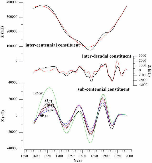
Core surface radial field and its constituents. Upper plot: black—gufm1 unfiltered time series of the radial core field (location of NGK observatory); red—the inter-centennial constituent. Middle plot: inter-decadal constituent of the core surface field; Butterworth (color, cutoff—22 years) and running averages (black, 22-year window) filters. Lower plot: sub-centennial constituent of the gufm1 core surface field; Butterworth (color) and running averages (black) filters (numbers on curves—the cutoff/window length)

Appendix 2: Sub-centennial constituent in Gauss coefficients of gufm1 model
The constituents of the core field are also to be found in the gufm1Gauss coefficients. In Fig. 9 we show the sub-centennial constituent obtained by means of running averages in several coefficients (n = 1, 2, 3). Besides the main period of 60–90 years, shorter ones and a certain expected degrading of amplitudes prior to 1840 are also seen in some cases. The phase differences are expected, as in predicting the field constituent, coefficients multiply by various functions of latitude and longitude to give location-dependent field values.

The sub-centennial constituent of gufm1 Gauss coefficients time evolution, degree n = 1, 2, 3
Rights and permissions
Open Access This article is distributed under the terms of the Creative Commons Attribution 4.0 International License (http://creativecommons.org/licenses/by/4.0/), which permits unrestricted use, distribution, and reproduction in any medium, provided you give appropriate credit to the original author(s) and the source, provide a link to the Creative Commons license, and indicate if changes were made.
About this article

Cite this article
Stefan, C., Dobrica, V. & Demetrescu, C. Core surface sub-centennial magnetic flux patches: characteristics and evolution. Earth Planets Space 69, 146 (2017). https://doi.org/10.1186/s40623-017-0732-1
Received:
Accepted:
Published:
DOI: https://doi.org/10.1186/s40623-017-0732-1