
Abstract
A two-species commensal symbiosis model involving Allee effect and one party can not survive independently is proposed and studied in this paper. Sufficient conditions which ensure the local and global stability of the boundary equilibrium and the positive equilibrium are obtained, respectively. Numeric simulations show that with the increasing of Alee effect, the system takes much longer time to reach its stable steady-state solution, though the Allee effect has no influence on the final density of the species. The Allee effect has instable effect on the system, however, such effect is controllable.
1 Introduction
The aim of this paper is to investigate the dynamic behaviors of the following two-species commensal symbiosis model involving Allee effect and one party can not survive independently, which takes the form
where \(a_{1}, b_{1}, c_{1}, a_{2}, b_{2}\), and u are all positive constants, \(x(t)\) and \(y(t)\) are the densities of the first and second species at time t, \(a_{1}\) is the death rate of the first species, \(a_{2}\) is the intrinsic growth rate of the second species, \(\frac{a_{2}}{b_{2}}\) is the environment carrying capacity of the second species. Also, the following assumptions are made in formulating model (1.1):
-
1.
The second species is favorable to the first species, while the first species has no influence on the second species;
-
2.
Without the help of the second species, the first species will be driven to extinction, i.e., the first species could not survive independently;
-
3.
We use the ratio-dependent functional response \(\frac{c_{1}y}{x+y}\) to describe the influence of the second species on the first species, where \(c_{1}\) describes the intensity of the cooperative effect of the second species on the first species;
-
4.
We incorporate the Allee effect \(\alpha(y) = \frac{y}{u+y}\) on the second species, such an Allee effect describes the fact of limitations in finding mates, which is also called weak Allee effect function. \(\alpha(y)\) is the probability of finding a mate where u is the individuals searching efficiency [1]. The bigger u is the stronger Allee effect is. By introducing the Allee effect, the per capita growth rate of the second species is reduced from
$$y (a_{2}-b_{2}y ) $$to
$$y (a_{2}-b_{2}y )\frac{y}{u+y}. $$
During the last decades, many scholars investigated the dynamic behaviors of the mutualism model or commensalism model, see [2–33] and the references cited therein. Such topics as the stability of the positive equilibrium [2, 4, 5, 11, 12, 14, 17, 19, 24, 27, 28], the persistence of the feedback control cooperative system [2, 6, 8–10, 20], the existence of the positive periodic solutions [15, 21, 23, 26], the existence of almost periodic solutions [22], etc. have been extensively investigated. However, only recently did scholars pay attention to the commensal symbiosis model with one party can not survive independently [26–31].
Zhu, Li, and Xu[28] for the first time proposed the following commensalism model:
where \(a_{1}<0\), \(a_{2}>0\), \(b_{1}<0\), \(b_{2}<0\), \(c_{1}>0\). Here, \(a_{1}<0\) means that the first species can not survive independently. By analyzing the vector field of system (1.2), the authors could give sufficient conditions which ensure local stability of the positive equilibrium and the boundary equilibrium, respectively.
Yang, Han, and Xue [29] generalized system (1.2) to the non-autonomous case, they investigated the dynamic behaviors such as the persistence, extinction, and stability property of the following two-species commensalism model:
where \(a_{1}(t), a_{2}(t), b_{1}(t), c_{1}(t), b_{2}(t)\) are all continuous functions bounded above and below by positive constants.
Corresponding to system (1.3), Chen, Pu, and Yang [26] and Chen, Lin, and Yang [30] proposed a discrete commensal symbiosis model
They investigated the existence of positive ω-periodic solution, the permanence, extinction, and global attractivity of the system.
All of the above systems used the assumption that the influence of the second species on the first one is linearizing. Recently, Wu and Lin [27] argued that a more suitable model should incorporate some functional response, which reflects the saturation effect. They proposed the following commensalism model with ratio-dependent functional response and one party can not survive independently:
For the autonomous case, they obtained sufficient conditions which ensure the existence, local and global stability property of the equilibria. For the non-autonomous case, sufficient conditions which ensure the permanence and global stability property of the system are obtained.
The Allee effect, which describes the fact that the phenomenon of reduced per-capita population growth rate at low densities can be caused by difficulties in finding a mate or predator, avoid danger or defense. As was pointed out by Wang, Zhang, and Liu [34], “The population goes extinct below a threshold and increases above the threshold of population density. The Allee effect is therefore important in conservation of endangered and exploited species.” During the last decades, many scholars studied the influence of Allee effect, see [1, 34–42] and the references cited therein. Kang and Yakuba [37] studied the population dynamics of a two-species discrete-time competition model where each species suffers from either predator saturation induced Allee effects or mate limitation induced Allee effects. Kang and Udiani [42] studied the dynamic behaviors of a single species with Allee effect. Some scholars [1, 40, 41] also considered the influence of Allee effect on the epidemic ecosystem.
Çelik and Duman[36] for the first time proposed the following two-species discrete predator–prey system, where the prey species suffers from mating induced weak Allee effect:
Their study showed that if the prey population is subjected to the Allee effect, the trajectory of the solutions approximates to the corresponding equilibrium point much faster. Also, in some cases, the equilibrium point moves from instability to stability.
Stimulated by the work of Çelik and Duman [36], Wang, Zhang, and Liu [34] proposed the following predator–prey system with predator suffering the Allee effect:
where \(\frac{P_{t}}{u+P_{t}}\) is the term for Allee effect, and u is the Alee effect constant. The bigger u is, the stronger the Allee effect will be. By calculating the Jacobean matrix, the authors obtained sufficient conditions which ensure the local asymptotic stability of the positive equilibrium of the system.
Hüseyin Merdan [38] investigated the influence of the Allee effect on the Lotka–Volterra type predator–prey system. To do so, the author proposed the following predator–prey system with Allee effect:
where \(\frac{x}{\beta+x}\) represents the Allee effect, β is a positive constant. He showed that the dynamic behaviors of system (1.7) are very different to those of system (1.6); more precisely: (1) The system subject to an Allee effect takes longer time to reach its steady-state solution; (2) The Allee effect reduces the population densities of both predator and prey at the steady state.
Recently, stimulated by the works of Çelik and Duman [36] and Wang, Zhang, and Liu [34], Ufuktepe, Kapcak, and Akman [35] considered the influence of Allee effect on predator species, and they proposed the following system:
The authors investigated the stability and invariant manifolds of the above system by using center manifold theory.
Noting that all the works of [34–36, 38] are about the predator–prey system, some scholars tried to propose and study other kinds of ecosystems, for example, Wu, Li, and Lin [39] proposed the following two-species commensal symbiosis model with Holling type functional response and the Allee effect on the second species:
where \(a_{i}, b_{i}, i=1,2\), p, u, and \(c_{1}\) are all positive constants, \(p\geq1\). The authors investigated the local and global stability property of the equilibria. They showed that the unique positive equilibrium is globally stable, the Allee effect has no influence on the final density of the species; Sasmal et al. [1] proposed and analyzed the following deterministic eco-epidemiological system where the susceptible pest exhibits a weak Allee effect due to mating limitation:
The reduction of disease eradication, and predator–pest coexistence is observed around the predator-free and disease-free equilibrium, respectively. They also showed that the interior equilibrium is always unstable.
Stimulated by the works of [1, 26–42], we propose system (1.1), where the second species is subjected to the Allee effect from the mating limitation.
We arrange the paper as follows. In the next section, we investigate the existence and local stability of the equilibria. In Sect. 3, we investigate the global stability property of boundary equilibrium and positive equilibrium of the system. In Sect. 4, an example together with its numeric simulations is presented to show the feasibility of our main results. We end this paper with a brief discussion.
2 The existence and local stability of the equilibria
The equilibria of system (1.1) are determined by the system
One may argue that system (1.1) admits the equilibrium \(O(0,0)\). However, since in the above system, in the term \(\frac{c_{1}y }{x+y }\), 0 as denominator is unrealistic, and we could not explain clearly the meaning of \(O(0,0)\), so in this paper, we will focus on the solution of the following system:
From (2.1), system (1.1) always admits the boundary equilibrium \(A_{1} (0, \frac{a_{2}}{b_{2}} )\). Also, if \(a_{1}< c_{1}\), then system (1.1) admits a unique positive equilibrium \(A_{2} (x^{*},y^{*} )\), where
Obviously, \(A_{2} (x^{*},y^{*} )\) satisfies the equation
Concerned with the local stability property of the above three equilibria, we have the following.
Theorem 2.1
\(A_{1} (0, \frac{a_{2}}{b_{2}} )\) is unstable if \(a_{1}< c_{1}\) and locally stable if \(a_{1}>c_{1}\); \(A_{2} (x^{*},y^{*} )\) is locally stable if \(a_{1}< c_{1}\).
Proof
The Jacobian matrix of system (1.1) is calculated as
where
Then the Jacobian matrix of system (1.1) about the equilibrium \(A_{1}(0, \frac{a_{2}}{b_{2}})\) is given by
The corresponding eigenvalues are
Obviously, if \(a_{1}>c_{1}\), then \(\lambda_{1}<0\), in this case, \(A_{2}(0, \frac{r_{2}}{a_{22}})\) is locally stable. And \(A_{1}(0, \frac{r_{2}}{a_{22}})\) is unstable if \(a_{1}< c_{1}\).
By using (2.3), the Jacobian matrix about the positive equilibrium \(A_{2}\) is given by
The eigenvalues of the above matrix are
Hence, \(A_{2}(x^{*}, y^{*})\) is locally stable.
This ends the proof of Theorem 2.1. □
3 Global stability of the equilibria
This section will further investigate the global stability property of the equilibria.
Lemma 3.1
([1])
Consider the following equation:
where \(a_{2}, b_{2}, u\) are all positive constants. Then the unique positive equilibrium \(y^{*}= \frac {a_{2}}{b_{2}}\) is globally stable.
Theorem 3.1
Assume that \(a_{1}>c_{1}\) holds, then \(A_{1} (0, \frac{a_{2}}{b_{2}} )\) is globally stable.
Proof
Noting that the second equation of (1.1) takes the form
By applying Lemma 3.1 to system (3.2), we know that system (3.2) has a unique globally stable positive equilibrium \(y^{*}=\frac{a_{2}}{b_{2}}\), i.e., \(\lim _{t\rightarrow+\infty}y(t)=y^{*}\).
From the first equation of system (1.1) and the nonnegativity of the solution of system (1.1), it immediately follows that
hence,
This ends the proof of Theorem 3.1. □
Theorem 3.2
Assume that \(a_{1}< c_{1}\) holds, then \(A_{2} (x^{*}, y^{*} )\) is globally stable.
Proof
In the proof of Theorem 3.1, we showed that \(\lim _{t\rightarrow+\infty}y(t)=\frac{a_{2}}{b_{2}}\). That is, for any \(\varepsilon>0\) small enough, there exists \(T>0\) such that, for all \(t>T\),
By using (3.5), from the first equation of system (1.1), similarly to the analysis of (3.4)–(3.9) of Wu and Lin [27], we could have
where
Equation (3.5) and (3.6) show that every solution of system (1.1) starting in \({R}^{2}_{+}\) is uniformly bounded on
Also, under the assumption of Theorem 3.2, Theorem 2.1 shows that there is a unique locally stable positive equilibrium \(A_{2}(x^{*}, y^{*})\). To show that \(A_{2}(x^{*}, y^{*})\) is globally stable, it is enough to show that the system admits no limit cycle in the area D. Let us consider the Dulac function \(u(x,y)=x^{-1}y^{-2}\), then
where
By Dulac theorem [33], there is no closed orbit in area D. Consequently, \(A_{2}(x^{*}, y^{*})\) is globally asymptotically stable. This completes the proof of Theorem 3.2. □
4 Numeric simulations
Now let us consider the following example, which is the modification of Example 5.1 of Wu and Lin [27].
Example 4.1
Consider the following system:
In this system, corresponding to system (1.1), we take \(b_{1}=c_{1}=a_{2}=b_{2}=1\).
-
(1)
Now take \(a_{1}=2\), \(u=0.5\), then \(a_{1}>c_{1}\), it follows from Theorem 3.1 that \((0,1)\) is globally stable. Numeric simulation (Fig. 1) supports this assertion.
Figure 1 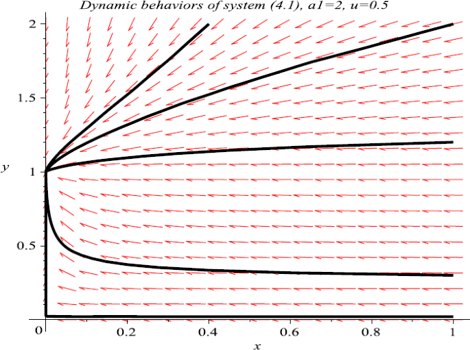
Numeric simulations of system (4.1) with \(a_{1}=2\), \(u=0.5\) and the initial conditions \((x(0), y(0))=(0.4, 2), (1, 0.3), (1, 0.02), (1, 2)\), and \((1,1.2)\), respectively

Now let us consider the influence of the parameter u. Let us take \(u=0.1, 0.5, 1\), respectively. Figure 2 and Fig. 3 show that in this case, parameter u has no influence on the final density of the species, i.e., the first species will be driven to extinction, while the second species will approach 1;
-
(2)
Now take \(a_{1}=\frac{1}{2}\), then \(a_{1}< c_{1}\), it follows from Theorem 3.2 that the unique positive equilibrium \((0.281,1)\) is globally stable. Numeric simulation (Fig. 4) supports this assertion.

Numeric simulations of \(x (t)\), with \(u=0.1, 0.5, 1\), where the black curve is the solution of \(u=1\), the green curve is the solution of \(u=0.1\), and the red curve is the solution of \(u=0.5\), and \((x(0),y(0))=(0.1, 0.2)\)

Numeric simulations of \(y (t)\), with \(u=0.1, 0.5, 1\), where the black curve is the solution of \(u=1\), the green curve is the solution of \(u=0.1\), and the red curve is the solution of \(u=0.5\), and \((x(0),y(0))=(0.1, 0.2)\)
Now let us consider the influence of the parameter u. Let us take \(u=0.1, 0.5, 1\), respectively. Figure 5 and Fig. 6 show that in this case, parameter u has no influence on the final density of both species.
5 Discussion
Based on a commensalism model proposed by Wu and Lin [27], we propose a two-species commensal symbiosis model involving Allee effect and one party can not survive independently. We show that the dynamic behaviors of system (1.1) coincide with those of system (1.5), i.e., if \(a_{1}>c_{1}\), that is, the intrinsic death rate of the first species is larger than the commensalism effect between the species, then the first species will be driven to extinction; and if \(a_{1}< c_{1}\), that is, the cooperative effect between two species is larger than the intrinsic death rate of the first species, then two species could coexist in a stable state.
For the case \(a_{1}>c_{1}\), the boundary equilibrium is globally stable, which means the extinction of the first species and the global attractivity of the second species (see Fig. 1). Numeric simulations (Fig. 2, Fig. 3) show that with the increasing of Allee effect (the increasing of u), the first species almost takes the same time to drive to extinction, while the second species needs much more time to reach its stable state.
For the case \(a_{1}< c_{1}\), the system admits a unique positive equilibrium, which is globally stable (see Fig. 4); however, numeric simulations (Fig. 5, Fig. 6) show that with the increasing of Allee effect (the increasing of u), the system needs much more time to reach its steady state.

Numeric simulations of system (4.1) with \(a_{1}=\frac{1}{2}\) and the initial conditions \((x(0), y(0))=(0.4, 2), (1, 0.3), (1, 0.02), (1, 2)\), and \((1,1.2)\), respectively

Numeric simulations of \(x(t)\), with \(u=0.1, 0.5, 1\), where the black curve is the solution of \(u=1\), the green curve is the solution of \(u=0.1\), and the red curve is the solution of \(u=0.5\), and \((x(0),y(0))=(0.1, 0.2)\)

Numeric simulations of \(y (t)\), with \(u=0.1, 0.5, 1\), where the black curve is the solution of \(u=1\), the green curve is the solution of \(u=0.1\), and the red curve is the solution of \(u=0.5\), and \((x(0),y(0))=(0.1, 0.2)\)
We mention here that a suitable system should incorporate some past state of the species, and this leads to a system with time delay, generally speaking, time delay may lead to the Hopf bifurcation or some other new phenomenon, we will leave this for future investigation.
References
Sasmal, S.K., Bhowmick, A.R., Khaled, K.A., Bhattacharya, S., Chattopadhyay, J.: Interplay of functional responses and weak Allee effect on pest control via viral infection or natural predator: an eco-epidemiological study. Differ. Equ. Dyn. Syst. 24(1), 21–50 (2015)
Yang, K., Miao, Z.S., Chen, F.D., Xie, X.D.: Influence of single feedback control variable on an autonomous Holling-II type cooperative system. J. Math. Anal. Appl. 435(1), 874–888 (2016)
Yang, K., Xie, X.D., Chen, F.D.: Global stability of a discrete mutualism model. Abstr. Appl. Anal. 2014, Article ID 709124 (2014)
Chen, F.D., Xie, X.D., Chen, X.F.: Dynamic behaviors of a stage-structured cooperation model. Commun. Math. Biol. Neurosci. 2015, Article ID 4 (2015)
Chen, F.D., Wu, H.L., Xie, X.D.: Global attractivity of a discrete cooperative system incorporating harvesting. Adv. Differ. Equ. 2016, 268 (2016)
Chen, L.J., Xie, X.D.: Feedback control variables have no influence on the permanence of a discrete N-species cooperation system. Discrete Dyn. Nat. Soc. 2009, Article ID 306425 (2009)
Xu, J.Y., Chen, F.D.: Permanence of a Lotka–Volterra cooperative system with time delays and feedback controls. Commun. Math. Biol. Neurosci. 2015, Article ID 18 (2015)
Chen, F.D., Yang, J.H., Chen, L.J., Xie, X.D.: On a mutualism model with feedback controls. Appl. Math. Comput. 214, 581–587 (2009)
Chen, L.J., Chen, L.J., Li, Z.: Permanence of a delayed discrete mutualism model with feedback controls. Math. Comput. Model. 50, 1083–1089 (2009)
Li, Y.K., Zhang, T.: Permanence of a discrete N-species cooperation system with time-varying delays and feedback controls. Math. Comput. Model. 53, 1320–1330 (2011)
Xie, X.D., Chen, F.D., Xue, Y.L.: Note on the stability property of a cooperative system incorporating harvesting. Discrete Dyn. Nat. Soc. 2014, Article ID 327823 (2014)
Xie, X.D., Chen, F.D., Yang, K., Xue, Y.L.: Global attractivity of an integrodifferential model of mutualism. Abstr. Appl. Anal. 2014, Article ID 928726 (2014)
Li, T.T., Chen, F.D., Chen, J.H., Lin, Q.X.: Stability of a stage-structured plant-pollinator mutualism model with the Beddington-DeAngelis functional response. J. Nonlinear Funct. Anal. 2017, Article ID 50 (2017)
Chen, F.D., Xie, X.D.: Study on the Dynamic Behaviors of Cooperation Population Modeling. Science Press, Beijing (2014)
Liu, Z.J., Wu, J.H., Tan, R.H., et al.: Modeling and analysis of a periodic delays two-species model of facultative mutualism. Appl. Math. Comput. 217, 893–903 (2010)
Yang, W.S., Li, X.P.: Permanence of a discrete nonlinear N-species cooperation system with time delays and feedback controls. Appl. Math. Comput. 218(7), 3581–3586 (2011)
Wu, R.X., Li, L., Zhou, X.Y.: A commensal symbiosis model with Holling type functional response. J. Math. Comput. Sci. 16, 364–371 (2016)
Lin, Q.F.: Dynamic behaviors of a commensal symbiosis model with non-monotonic functional response and non-selective harvesting in a partial closure. Commun. Math. Biol. Neurosci. 2018, Article ID 4 (2018)
Yang, L.Y., Xie, X.D., Chen, F.D.: Dynamic behaviors of a discrete periodic predator–prey-mutualist system. Discrete Dyn. Nat. Soc. 2015, Article ID 247269 (2015)
Han, R.Y., Chen, F.D.: Global stability of a commensal symbiosis model with feedback controls. Commun. Math. Biol. Neurosci. 2015, Article ID 15 (2015)
Xie, X.D., Miao, Z.S., Xue, Y.L.: Positive periodic solution of a discrete Lotka-Volterra commensal symbiosis model. Commun. Math. Biol. Neurosci. 2015, Article ID 2 (2015)
Xue, Y.L., Xie, X.D., Chen, F.D., Han, R.Y.: Almost periodic solution of a discrete commensalism system. Discrete Dyn. Nat. Soc. 2015, Article ID 295483 (2015)
Miao, Z.S., Xie, X.D., Pu, L.Q.: Dynamic behaviors of a periodic Lotka–Volterra commensal symbiosis model with impulsive. Commun. Math. Biol. Neurosci. 2015, Article ID 3 (2015)
Chen, J.H., Wu, R.X.: A commensal symbiosis model with non-monotonic functional response. Commun. Math. Biol. Neurosci. 2017, Article ID 5 (2017)
Chen, F.D., Xie, X.D., Miao, Z.S., et al.: Extinction in two species nonautonomous nonlinear competitive system. Appl. Math. Comput. 274, 119–124 (2016)
Chen, F.D., Pu, L.Q., Yang, L.Y.: Positive periodic solution of a discrete obligate Lotka-Volterra model. Commun. Math. Biol. Neurosci. 2015, Article ID 14 (2015)
Wu, R., Lin, L.: Dynamic behaviors of a commensal symbiosis model with ratio-dependent functional response and one party can not survive independently. J. Math. Comput. Sci. 16, 495–506 (2016)
Zhu, Z.F., Li, Y.A., Xu, F.: Mathematical analysis on commensalism Lotka–Volterra model of populations. J. Chongqing Institute of Technology (Natural Science Edition) 21(10), 59–62 (2007)
Yang, L.Y., Han, R.Y., Xue, Y.L.: On a nonautonomous obligate Lotka–Volterra model. J. Sanming University 31(6), 15–18 (2014)
Chen, F.D., Lin, C.T., Yang, L.Y.: On a discrete obligate Lotka–Volterra model with one party can not survive independently. J. Shenyang University(Natural Science) 27(4), 336–338 (2015)
Li, T.T., Lin, Q.X., Chen, J.H.: Positive periodic solution of a discrete commensal symbiosis model with Holling II functional response. Commun. Math. Biol. Neurosci. 2016, Article ID 22 (2016)
Chen, L.S., Song, X.Y., Lu, Z.Y.: Mathematical Models and Methods in Ecology. Shichuan Science and Technology Press, Chengdu (2002)
Zhou, Y.C., Jin, Z., Qin, J.L.: Ordinary Differential Equation and Its Application. Science Press, Beijing (2003)
Wang, W.X., Zhang, Y.B., Liu, C.Z.: Analysis of a discrete-time predator–prey system with Allee effect. Ecol. Complex. 8, 81–85 (2011)
Ufuktepe, U., Kapcak, S., Akman, O.: Stability and invariant manifold for a predator–prey model with Allee effect. Adv. Differ. Equ. 2013, 348 (2013)
Çelik, C., Duman, O.: Allee effect in a discrete-time predator–prey system. Chaos Solitons Fractals 90, 1952–1956 (2009)
Kang, Y., Yakubu, A.A.: Weak Allee effects and species coexistence. Nonlinear Anal., Real World Appl. 12, 3329–3345 (2011)
Merdan, H., Duman, O.: On the stability analysis of a general discrete-time population model predation and Allee effects. Chaos Solitons Fractals 40, 1169–1175 (2009)
Wu, R.X., Li, L., Lin, Q.F.: A Holling type commensal symbiosis model involving Allee effect. Commun. Math. Biol. Neurosci. 2018, Article ID 6 (2018)
Kang, Y., Sasmal, S.K., Bhowmick, A.R., Chattopadhyay, J.: A host-parasitoid system with predation-driven component Allee effects in host population. J. Biol. Dyn. 9, 213–232 (2014)
Sasmal, S.K., Chattopadhyay, J.: An eco-epidemiological system with infected prey and predator subject to the weak Allee effect. Math. Biosci. 246(2), 260–271 (2013)
Kang, Y., Udiani, O.: Dynamics of a single species evolutionary model with Allee effects. J. Math. Anal. Appl. 418, 492–515 (2014)
Acknowledgements
The author is grateful to three anonymous referees for their excellent suggestions, which have greatly improved the presentation of the paper.
Funding
This work is supported by the National Social Science Foundation of China (16BKS132), Humanities and Social Science Research Project of Ministry of Education Fund (15YJA710002), and the Natural Science Foundation of Fujian Province (2015J01283).
Author information
Authors and Affiliations
Contributions
All authors contributed equally to the writing of this paper. All authors read and approved the final manuscript.
Corresponding author
Ethics declarations
Competing interests
The authors declare that there is no conflict of interests.
Additional information
Publisher’s Note
Springer Nature remains neutral with regard to jurisdictional claims in published maps and institutional affiliations.
Rights and permissions
Open Access This article is distributed under the terms of the Creative Commons Attribution 4.0 International License (http://creativecommons.org/licenses/by/4.0/), which permits unrestricted use, distribution, and reproduction in any medium, provided you give appropriate credit to the original author(s) and the source, provide a link to the Creative Commons license, and indicate if changes were made.
About this article

Cite this article
Chen, B. Dynamic behaviors of a commensal symbiosis model involving Allee effect and one party can not survive independently. Adv Differ Equ 2018, 212 (2018). https://doi.org/10.1186/s13662-018-1663-2
Received:
Accepted:
Published:
DOI: https://doi.org/10.1186/s13662-018-1663-2