
Abstract
Map-matching is the process of matching the GPS locus to the road network on the digital map. However, due to the most existing map-matching algorithms that are based on high sampling rate, when the sampling interval is increased, the correct rate of the algorithm will be greatly reduced. Based on this, this paper proposed a new algorithm of map-matching for low sampling rate GPS trajectories. The algorithm gave full consideration to the road network of the geometric structure and topological structure and the mutual influence between adjacent points (time, speed information) by calculating the probability of each trajectory point of candidate points to determine matching results. At the end of this paper, we use the data of Beijing UCAR Inc.’s car in a case study. This case demonstrates: For low sampling rate matching track points in the complex road, the algorithm has a good uptime, and an exact match was found.
1 Introduction
As the result of maturity development of the Internet technology, the wisdom city can be built and developed quickly, including intelligent transportation infrastructure as one, which is indispensable. The construction of intelligence transportation includes several areas: vehicle navigation, traffic flow analysis, and satellite positioning which has not been intensively studied. All these mentioned application programs are based on the track. Its core steps are involved in GPS to accurately position the GPS track data of vehicles on the road, in other words, the map-matching [1].
Typical GPS track points data is a serious of sequential track points. Each GPS point consists of latitude, longitude, and timestamp information. However, on account of the limitation of the GPS itself, the sampling and measuring process of GPS data and the return or accept process of the measuring data will have possible errors, which further lead to inaccurate GPS data [2]. Therefore, the original data need to be processed and then be used on the road network, that is to say, the map-matching.
2 Application conditions of the algorithm
With the development of science and technology, the number of any travel navigation system has increased sharply, such as a GPS-embedded PAD and smartphone. Due to the spread of these devices, a large number of track point data can be available. But in the practice of real life, only a low sampling rate (e.g., a sample point every 2 min) of GPS can be obtained because of energy consumption, cost consumption, and so on. For example, there are more than 60,000 taxis in Beijing, and most of them are equipped with GPS [3, 4]. Usually, the taxi drivers drive on the road. In order to save energy consumption, the time intervals of their passing the GPS point is bound to increase, which leads to lower sampling rate of GPS track data [5, 6].
However, at present, the algorithm of map-matching is only for processing GPS data with high sampling rate (usually 10~30 s every one track point) [7]. When they use points with low sampling rate as their data, the matching error is over 50% [8, 9]. Therefore, in view of the track point with a low sampling point, the paper will put forward an improved algorithm of map-matching. Besides, the low sampling rate here means collecting one track point every 1.5 min and more [10, 11].
3 The algorithm design
Map-matching system of GPS navigation based on a low sampling rate consists of four parts: the preparation of candidate point, the analysis with the time factors, the analysis with the spatial factors, and the result matching.
3.1 The preparation of candidate point
The algorithm will give full consideration to the geometric structure of road network, so as to calculate the candidate point of the track point. It needs two steps to achieve this goal. Firstly, we have to find out the possible section of the track point, in other words, the candidate sections. Secondly, we have to calculate the candidate points in the section by making use of the point-to-curve in the present geometric map-matching algorithm.
-
1.
Selection of candidate sections: To find track points possible in sections, complete algorithm can be designed to allow each locus point for the entire network of roads to traverse, but this approach will lead to too much time complexity. Therefore, the algorithm must narrow the range of the segment to be compared. Existing algorithms use the error oval method in probability theory to narrow the comparison range of the road. However, the disadvantage of this method is that, it is very likely that there is no road node in the error ellipse, and people mistakenly believe that there is no candidate road segment. Therefore, this paper proposed a GeoHash algorithm to implement this step: through a certain rule [12, 13], a string to represent the latitude and two longitude coordinates.
-
2.
Calculating candidate points: After acquiring the perimeter of each GPS point, the algorithm calculates the candidate points of the GPS point on each link. From the track point to the section of the vertical line, if the foot points on the road section, the foot-point is the candidate point; if the foot-down point is not on the road, then select the nearest road segment endpoint as a candidate point.
-
3.
Filtering of candidate points: You may encounter the following problems during the last part of the search for candidate points: GeoHash algorithm can be found out by more than one road. Based on the existing map-matching algorithm geometry, it shows that if the distance between the candidate points and the locus of points are closer, the greater the likelihood of the candidate point is the best match point. Based on this, the algorithm stores only the first five candidate points, and the segments where the distance between the candidate points and the track points is the smallest in the database.
3.2 Spatial analysis
In this step, we need to make the most of the geometry and topology information of road network to evaluate the candidate point getting from the first step. In this paper, geometry information is represented by the observation density, and topology information is represented by transmission probability. Based on this algorithm, two hypotheses are proposed:
-
1.
Vehicles tend to run straight on the same road rather than bypass: Consider a taxi’s trajectory in Fig. 1. A taxi on the horizontal road e 1 from west to east, where P a, P b, and P c for the vehicle to move back in the process of three GPS location trajectory points. According to most of the current map-matching algorithm, the vertical distance of the path e 2 from the point P b to the vertical direction is smaller than the foot-up distance of the path e 1 from the point P b to the horizontal direction. Thus, the point P b is matched to e 2. But with the P b point before and after the two points P a and P c movement trends, it can be speculated that the taxi is not likely to take a roundabout way, that is, starting from e 1 to e 2 and then back to e 1. This example means that if the algorithm combines the location of the trajectory with the topology information of the road network, a better matching effect may be obtained.
Fig. 1 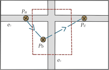
Trajectory of a vehicle on a horizontal road
-
2.
The speed of the vehicle is often limited by the maximum speed of the road on which it travels: Consider a taxi’s trajectory in Fig. 2, that is, traveling from south to north. During this time, the taxi returns a GPS track with two GPS locations which are P a and P b. If there is no velocity information for vehicle travel, it is almost impossible to distinguish whether the two track points belong to the highway e 1 or the ordinary road e 2. However, if the average speed of the travel process is calculated to be 80 km/h using the distances and timestamps of points P a and P b, it is entirely possible to determine that these two GPS trajectory points are likely to be on the highway e 1. This example illustrates that making good use of the time information and vehicle speed information can effectively improve the map-matching accuracy [14].
Fig. 2 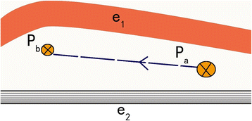
Vehicle longitudinal trajectories


3.3 Time analysis
In most cases, the algorithm can find out the best candidate point through spatial analysis, so that choosing the true path P i among the candidate paths { P i − 1, P i … P n } will be possible. However, there is a special kind of situation that cannot be solved by the spatial analysis, as shown in Fig. 3. In this figure, a thick yellow line stands for highway and a thin blue line represents the common roads. The two roads are very close, so if we use spatial analysis to calculate the candidate point of P i − 1 and P i , the results of the algorithm of two roads may be same. But if the average speed from P i − 1 to P i is 85 km/h, the two track points can be matched on the highway because of road speed limits. Therefore, it needs the time analysis of track points.

Influence factors of track point matching time speed information
Firstly, the algorithm needs to calculate the average speed \( \overline{v} \) from P i − 1 to P i ; the formula is as follows:
The candidate point of P i − 1 is C i − 1, the candidate point of P i is C i , and the shortest path from C i − 1 to C i is a series of sections [ e 1 ', e 2 '. .. e k ']. Therefore, the l u = e u '. l in the formula, that is, l u , is the length of e u '; the member means the shortest length from C i − 1 to C i ; and the denominator Δt i − 1 → i means the time intervals from P i − 1 to P i .
The algorithm thinks that every section e u ' in the road network has its own speed constraint value e u '. v. This paper will use cosine calculation to describe the similarity between the average speed from C i − 1 to C i and the section constraint value e u '. v. Therefore, the time analysis using time and speed information is defined as follows:
3.4 The result matching
After spatial matching, the paper can find out a candidate graph G ' (V ', T ') to its given track sequence T : P 1 → P 2 → … → P n . V ' is the candidate point of the track point; T ' is the side represented by the shortest path between two adjacent candidate points.
Every candidate point in the candidate graph G ' can be described by \( N\left({C}_i^s\right) \). Every side can be described by \( V\left({C}_{i-1}^t\to {C}_i^s\right) \) and \( {F}_t\left({C}_{i-1}^t\to {C}_i^s\right) \). To sum up, the paper can define the probability function of the map-matching as follows:
At last, we can get a candidate path collection from the whole track (T)—P c \( P:{C}_1^{S_1}\to {C}_2^{S_2}\to \dots \to {C}_n^{S_n} \). If to calculate each path’s value F(p c ), \( F\left({P}_c\right)={\displaystyle {\sum}_{i=2}^n F\left({c}_{i-1}^{S_{i-1}}\to {C}_i^{S_i}\right)} \),the maximum will be the final matching path.
4 The experimental results and analysis of the algorithm
Based on the algorithm proposed in this paper, using the true data of road network and track network, the experiment can be designed and made successfully. The experimental data includes road network data and track data. Using the road network in Beijing and downloading from the open source OpenStreetMap, the road network contains 112 sections and 74 road network sites. The track data came from the true Shenzhou taxi GPS track data provided by the Shenzhou Taxi Company. The formats of the GPS track data have four columns. The first column of data represents the longitude of the driving point, the second column of data represents the latitude, the third represents the speed of the vehicle, the fourth represents the point of view, and the last represents the timestamp. The overall effect of the final matching of the experiment is shown in Fig. 4, and the right part of the figure is the local magnification effect. The purple line is the track point sequence of the effect figure before matching, and the blue line is the track point sequence after matching.

Experimental matching effects
-
1.
Matching precision: In the experiment, there are about 1089 track points matching correctly on the roads, namely, the algorithm in this case can make the matching accuracy reach above 80%. Most of the 20% false match points distributed in turning points. Therefore, the next step may be for special sections at these points, the special design matching algorithm to improve the overall matching and accuracy matching algorithm.
-
2.
Matching time: In this case, the track point n is 1354, and the section of road network m is 112. According to the theoretical calculation complexity formula, the algorithm operation time in this experiment is 3.2 min.
-
3.
The effect of the number of trajectory points on time complexity: In this experiment, the control variable method is adopted, and the number of trajectory candidate points is taken as 5; only the number of trajectory points is changed, and the matching running time under a different number of trajectory points is calculated. The results of the experiment showed the number of points at the candidate locus of points in certain circumstances; the purpose of increasing the number of points on the trajectory program run time is not large but always controlled within a certain range.
-
4.
The influence of the maximum number of candidate points of track points on time complexity: In this experiment, the number of points to ensure that the trajectory remains unchanged and the number of candidate points were used by changing only the trace points to analyze the impact of its running time; it was found that with the increase in the number of candidate points, with the increase in the running time, and when the number of candidate points is over 5, the running time surges. If the number of candidate point values is too small, it will lead to lower matching accuracy. Therefore, in this algorithm, the number of candidate points that the trajectory point has at most is determined as 5 by combining the running time and the matching precision.
5 Conclusions
In view of the limitation of energy and resources in real life, the actual sampling intervals of getting GPS trajectories is very large, while the existing map-matching algorithms are aimed at a high sampling rate. Therefore, this paper proposed a special map-matching algorithm aiming at GPS trajectories with a low sampling rate. Probabilistic matching is taken as the core idea, and the probabilistic calculation of each trajectory point is carried out considering the road network geometry (observation probability), the topological structure (transmission probability), and the time speed information of vehicles (spatial analysis). The best matching point is determined by calculating the result. Finally, the paper verifies the matching precision of algorithm and time complexity through experimental analysis with actual data. This method can be applied to the map navigation system as a supplement. When calculating the shortest path adjacent track points between the candidate points, for convenience, we use Dirjkstra algorithm. But for the shortest path calculation, Dirjkstra algorithm is not the most effective way when the algorithm uses A* algorithm or ATL algorithm, which can often improve the running time of the algorithm. Therefore, the algorithm can also do some improvements for this part of the algorithm in most path calculations.
Change history
04 September 2017
An erratum to this article has been published.
References
P. Misra, P. Pratap, Global positioning system: signals, measurements, and performance. Ganga-Jamuna Press. 1(2):83-105 (2011)
AM Pinto, AP Moreira, PG Costa, A localization method based on map-matching and particle swarm optimization. J. Intell. Robot. Syst. 77(2), 313–326 (2015)
Shi A N, Kuang W M. Research on Taxi GPS Trajectory Composing Method[J]. Sci. Technol. Eng. 15(11), 125–130 (2015)
H Fan, B Du, Reasonable Quantities Evaluation of Megalopolis Taxicab and Its Realizing Methods:Evidence from Beijing. Res. Econ. Manag. 36(8), 91–94 (2015)
Z. Li, L. Song, H. Shi, Approaching the capacity of K-user MIMO interference channel with interference counteraction scheme. Ad Hoc Networks. 2016. DOI:10.1016/j.adhoc.2016.02.009.
Z Li, K Liu, Y Zhao, Y Ma, MaPIT: an enhanced pending interest table for NDN with mapping bloom filter. IEEE Commun. Lett. 18(11), 1423–1426 (2014). doi:10.1109/LCOMM.2014.2359191
Y. Zheng, L. Capra, O. Wolfson, H. Yang, Urban Computing: concepts, methodologies, and applications. ACM Trans. Intell. Syst. Technol. 5(3):38 (2014)
Peker, Ali Ufuk, O. Tosun, and T. Acarman. "Particle filter vehicle localization and map-matching using map topology." Intelligent Vehicles Symposium IEEE Xplore. 2011:248-253
S. Lamy-Perbal, N. Guenard, M. Boukallel, et al, "A HMM map-matching approach enhancing indoor positioning performances of an inertial measurement system."International Conference on Indoor Positioning and Indoor Navigation. 2015:1-4
Giovannini, Luca. "A novel map-matching procedure for low-sampling GPS data with applications to traffic flow analysis." Universita Di Bologna. (2011)
Z Li, Y Chen, H Shi, K Liu, NDN-GSM-R: a novel high-speed railway communication system via named data networking. EURASIP J. Wirel. Commun. Netw. 2016(48), 1–5 (2016). doi:10.1186/s13638-016-0554-z
M Srivatsa, R Ganti, J Wang et al., Map matching: facts and myths[C]// ACM Sigspatial International Conference on Advances in Geographic Information Systems, 2013, pp. 484–487
X. Liu, Z. Li, P. Yang, Y. Dong, Information-centric mobile ad hoc networks and content routing: A survey. Ad Hoc Netw. (2016). http://dx.doi.org/10.1016/j.adhoc.2016.04.005
D Chen, L Chen, J Liu et al., Road link traffic speed pattern mining in probe vehicle data via soft computing techniques[J]. Appl. Soft Comput. 13(9), 3894–3902 (2013)
Acknowledgements
This research was supported by National Natural Science Foundation of China (61602346).
Authors' contributions
YL conceived of this algorithm study and participated in its design and coordination. ZL participated in the design of this algorithm study and performed the experiment analysis. Both authors read and approved the final manuscript.
Competing interests
The authors declare that they have no competing interests.
Author information
Authors and Affiliations
Corresponding author
Additional information
An erratum to this article is available at https://doi.org/10.1186/s13638-017-0933-0.
Rights and permissions
Open Access This article is distributed under the terms of the Creative Commons Attribution 4.0 International License (http://creativecommons.org/licenses/by/4.0/), which permits unrestricted use, distribution, and reproduction in any medium, provided you give appropriate credit to the original author(s) and the source, provide a link to the Creative Commons license, and indicate if changes were made.
About this article

Cite this article
Liu, Y., Li, Z. A novel algorithm of low sampling rate GPS trajectories on map-matching. J Wireless Com Network 2017, 30 (2017). https://doi.org/10.1186/s13638-017-0814-6
Received:
Accepted:
Published:
DOI: https://doi.org/10.1186/s13638-017-0814-6