
Abstract
Nahm sums are q-series of a special hypergeometric type that appear in character formulas in the conformal field theory, and give rise to elements of the Bloch group, and have interesting modularity properties. In our paper, we show how Nahm sums arise naturally in the quantum knot theory - we prove the stability of the coefficients of the colored Jones polynomial of an alternating link and present a Nahm sum formula for the resulting power series, defined in terms of a reduced diagram of the alternating link. The Nahm sum formula comes with a computer implementation, illustrated in numerous examples of proven or conjectural identities among q-series.
MSC
Primary 57N10; Secondary 57M25.
1 Background
The colored Jones polynomial of a link is a sequence of Laurent polynomials in one variable with integer coefficients. We prove in full a conjecture concerning the stability of the colored Jones polynomial for all alternating links.
A weaker form of stability (zero stability, defined below) for the colored Jones polynomial of an alternating knot was conjectured by Dasbach and Lin. The zero stability is also proven independently by Armond for all adequate links [1], which include alternating links and closures of positive braids, see also [2]. The advantage of our approach is that it proves stability to all orders and gives explicit formulas (in the form of generalized Nahm sums) for the limiting series, which in particular implies convergence in the open unit disk in the q-plane and allow for the study of their redial asymptotics.
Stability was observed in some examples by Zagier, and conjectured by the first author to hold for all knots, assuming that we restrict the sequence of colored Jones polynomials to suitable arithmetic progressions, dictated by the quasi-polynomial nature of its q-degree [3, 4]. Zagier asked about modular and asymptotic properties of the limiting q-series. In a similar direction, Habiro asked about zero stability of the cyclotomic function of alternating links in [5].
Our generalized Nahm sum formula comes with a computer implementation (using as input a planar diagram of a link), and allows the study of its asymptotics when q approaches radially a root of unity. Our Nahm sum formula is reminiscent to the cohomological Hall algebra of motivic Donaldson-Thomas invariants of Kontsevich-Soibelman [6] and complement recent work of Witten [7] and Dimofte-Gaiotto-Gukov [8].
1.1 Nahm sums
Recall the quantum factorial and quantum Pochhammer symbol defined by [9]

We will abbreviate (x;q) n by (x) n .
In [10], Nahm studied q-hypergeometric series  of the form

where A is a positive definite even integral symmetric matrix and  .
.
Nahm sums appear in character formulas in the conformal field theory, and define analytic functions in the complex unit disk |q|<1 with interesting asymptotics at complex roots of unity, and with sometimes modular behavior. Examples of Nahm sums are the seven famous, mysterious q-series of Ramanujan that are nearly modular (in modern terms, mock modular). For a detailed discussion, see [11]. Nahm sums give rise to elements of the Bloch group, which governs the leading radial asymptotics of f(q) as q approaches a complex root of unity. Nahm’s conjecture concerns the modularity of a Nahm sum f(q), and was studied extensively by Zagier, Vlasenko-Zwegers and others [12, 13].
The limit of the colored Jones function of an alternating link leads us to consider generalized Nahm sums of the form

where C is a rational polyhedral cone in  ,
,  and A is a symmetric (possibly indefinite) symmetric matrix. We will say that the generalized Nahm sum (1) is regular if the function

is proper and bounded below. Regularity ensures that the series (1) is a well-defined element of the Novikov ring

of power series in q with integer coefficients and bounded below minimum degree. In the remaining of the paper, by Nahm sum we will mean a generalized Nahm sum. The paper is concerned with a new source of Nahm sums that originate in the quantum knot theory.
1.2 Stability of a sequence of polynomials
For  let mindeg
q
f(q) denote the smallest j such that a
j
≠0 and let coeff(f(q),q
j)=a
j
denote the coefficient of q
j in f(q).
let mindeg
q
f(q) denote the smallest j such that a
j
≠0 and let coeff(f(q),q
j)=a
j
denote the coefficient of q
j in f(q).
Definition 1
Suppose  . We write that

if
-
there exists C such that mindeg q (f n (q))≥C for all n, and
-
for every
 ,
,
 (2)
(2)
 ,
,

Since Equation 2 involves a limit of integers, the above definition implies that for each j, there exists N j such that

(and in particular, coeff(f n (q),q j)=coeff(f(q),q j)) for all n>N j .
Remark 1
Although for every integer j we have  , it is not true that
  .
.
Definition 2
A sequence  is k-stable if there exist
  for j=0,…,k such that

We say that (f n (q)) is stable if it is k-stable for all k. Notice that if f n (q) is k-stable, then it is k ′-stable for all k ′<k and moreover Φ j (q) for j=0,…,k is uniquely determined by f n (q). We call Φ k (q) the k-limit of (f n (q)). For a stable sequence (f n (q)), its associated series is given by

It is easy to see that the pointwise sum and product of k-stable sequences are k-stable.
1.3 Stability of the colored Jones function for alternating links
Given a link K, let  denote its colored Jones polynomial (see e.g. [14, 15]) with each component colored by the (n+1)-dimensional irreducible representation of
  and normalized by

When K is an alternating link, the lowest degree of J
K,n
(q) is known and the lowest coefficient is ±1 (see [16, 17] and Section 7). We divide J
K,n
(q) by its lowest monomial to obtain  . Although
  , we have
  ; see [18].
Our main results link the colored Jones polynomial and its stability with Nahm sums. The first part of the result, with proof given in Section 9, is the following:
Theorem 1
For every alternating link K, the sequence  is stable and its associated k-limit Φ
K,k
(q) and series F
K
(x,q) can be effectively computed from any reduced, alternating diagram D of K.
is stable and its associated k-limit Φ
K,k
(q) and series F
K
(x,q) can be effectively computed from any reduced, alternating diagram D of K.
Let us give some remarks regarding Theorem 1.
Remark 2
If one uses the new normalization where with J Unknot,n (q)=1, the above theorem still holds. The new F K (x,q) is equal to the old one times (1−q)/(1−x).
Remark 3
If  is the mirror image of K, then
  . If K is alternating, then so is
  . Hence, applying Theorem 1 to
  , we see that similar stability result holds for the head of the colored Jones polynomial of alternating link.
Remark 4
The weaker zero stability (conjectured by Dasbach and Lin) is proven independently by Armond [2]. In [2], zero stability is proved for all A-adequate links, which include all alternating links, but no stability in full is proven there, nor any formula for the zero limit is given. As we will see, the proof of stability in full is more complicated than that of zero stability and occupies the more difficult part of our paper, given in Sections 8 to 10.
Remark 5
A sharp estimate regarding the rate of convergence of the stable sequence  is given in Theorem 4.
1.4 Explicit Nahm sum formulas for the zero limit and one limit
Throughout this subsection, D is a reduced diagram of a non-split alternating link K with c crossings.
1.4.1 Laplacian of a graph
In this paper, a graph is a finite one-dimensional CW-complex. A plane graph is a graph Γ (with loops and multiple edges allowed) together with an embedding of Γ into  . A plane graph Γ gives rise to a polygonal complex structure of S
2, and its set of vertices, set of edges, and set of polygons are denoted respectively by
. A plane graph Γ gives rise to a polygonal complex structure of S
2, and its set of vertices, set of edges, and set of polygons are denoted respectively by  ,
,  and
and  .
.
The adjacency matrix Adj(Γ) is the  matrix defined such that Adj(Γ)(v,v
′) is the number of edges connecting v and v
′. Let Deg(G) be the diagonal
matrix defined such that Adj(Γ)(v,v
′) is the number of edges connecting v and v
′. Let Deg(G) be the diagonal  matrix such that Deg(Γ)(v,v) is the degree of the vertex v, i.e. the number of edges incident to v, with the convention that each loop edge at v is counted twice.
The Laplacian
 plays an important role in graph theory.
1.4.2 Graphs associated to a reduced alternating non-split link diagram D
The diagram D gives rise to a polygonal complex of  with c vertices, 2c edges, and c+2 polygons. Since D is alternating, there is a way to assign a color A or B to each polygon such that in a neighborhood of each crossing the colors are as in Figure 1, see e.g. [19, p.217].

A checkerboard coloring of alternating planar projections.
This is the usual checkerboard coloring of the regions of an alternating link diagram, used already by Tait. When we rotate the overcrossing arc at a crossing counterclockwise (resp. clockwise), we swap an A-type (resp. B-type) angle. Note that orientation dose not take part in the definition of A-angles and B-angles.
Let D
∗ be the dual of the plane graph D. Since D has a checkerboard coloring of its faces, it follows that D
∗ has a coloring of its vertices by A or B. Thus,  give a bipartite structure on
  where
where  and
and  are the sets of A-colored and B-colored vertices of
  .
.
Since the degree of each vertex of D is 4, each polygon of D
∗ is a quadrilateral, having four vertices, two of which are A vertices and two are B vertices. Moreover, the vertices of each quadrilateral alternate in color. Connect the two B vertices of each quadrilateral of D
∗ by a diagonal inside that quadrilateral, and call it a  -edge. The Tait graph of D is defined to be the plane graph
  whose set of vertices is
  , and whose set of edges is the set of
  -egdes. The plane graph Tait graph totally determines the alternating link K up to orientation. The graph
  can be defined for any link diagram, and is studied extensively, see e.g. [20]-[22].
Note that for a vertex  , its degrees in D
∗ and in
, its degrees in D
∗ and in  are the same.
1.4.3 The lattice and the cone
Fix an A-vertex of D
∗ and call it v
∞
. We will focus on  , the
, the  -lattice of rank c+2 freely spanned by the vertices of D
∗. Let
-lattice of rank c+2 freely spanned by the vertices of D
∗. Let  , a sublattice of Λ of rank c+1.
For an edge  , define the
  -linear map
  by
by

An element x∈Λ
0 is admissible if e(x)≥0 for every edge  . The set Adm⊂Λ
0 of all admissible elements is the intersection of Λ
0 with a rational convex cone in
. The set Adm⊂Λ
0 of all admissible elements is the intersection of Λ
0 with a rational convex cone in  .
.
Define the  -linear map
  by
by

Let  be the symmetric
  matrix defined by

Note that a priori
 is a
is a  matrix, and is considered as a
  matrix in the right-hand side of (4) by the trivial extension, i.e. in the extension, any entry outside the block
  is 0.
is 0.
The symmetric matrix  defines a symmetric bilinear form
  . Let
. Let  be the corresponding quadratic form, i.e.

Remark 6
Although Q(λ) and L(λ) take value in  , we later show that
  . While Q,L depend only on D, the set Adm depends on the choice of an A-vertex v
∞
.
. While Q,L depend only on D, the set Adm depends on the choice of an A-vertex v
∞
.
Examples that illustrate the above definitions are given in Section 1.6.
1.4.4 Nahm sum for the zero limit
The next theorem is proven in Section 7.
Theorem 2.
Suppose D is a reduced alternating diagram of a non-split link K. Fix any choice of v
∞
. Then the zero limit of  is equal to

The generalized Nahm sum on the right-hand side is regular and belongs to  .
.
A categorification of the above theorem was given recently by Rozansky [23]. Here are two consequences of this explicit formula. The next corollary is proven in Section 7.4.
Corollary 1
For every alternating link K,  is analytic in the unit disk |q|<1.
The next corollary is shown in Section 13.
Corollary 2
If the reduced Tait graphs of two alternating links K
1,K
2 are isomorphic as abstract graphs, then they have the same zero limit,  .
.
Here the reduced Tait graph  is obtained from
  by replacing every set of parallel edges by an edge; and two edges are parallel if they connect the same two vertices. This corollary had been proven by Armond and Dasbach: in [24], it is proved that if two alternating links have the same reduced Tait graph, and the zero limit of the first link exists, then the zero limit of the second one exists and is equal to that of the first one. In Section 13, we will derive Corollary 2 from the explicit formula of Theorem 2.
We end this section with a remark on normalizations.
Remark 7
The colored Jones polynomial J
K,n
(q) (and consequently, its shifted version  ) is independent of the orientation of the components of a link K[25]. With our normalization we have

where ⊔ and ♯ denotes the disjoint union and the connected sum respectively.
1.4.5 The one limit
For a quadrilateral p of D
∗, define a  -linear map
  by
by

The next theorem is proven in Section 12.2.
Theorem 3.
Suppose D is a reduced alternating diagram of a non-split link L. Fix any choice of v
∞
. The one limit of  is
is

where Admv is the set of all admissible x such that p(x)=0 for every  incident to v.
Remark 8
The fact that the series (6) is convergent is not obvious. It follows from the fact that we can separate the sum over admissible states λ to those which are not one-bounded and those which are one-bounded. Here, a state λ is one-unbounded if  ; see Definition 5. It is easy to see that the contribution of the one-unbounded states in (6) forms a convergent series. For the one-bounded states s, one uses a decomposition theorem s=m
s
P
+s
′ discussed in Example 2. Then, the contribution of such a state to (6) comes with minimum degree Q(s
′)+L(s
′)+m. This implies that the contribution of the one-bounded states in (6) forms a convergent series too.
; see Definition 5. It is easy to see that the contribution of the one-unbounded states in (6) forms a convergent series. For the one-bounded states s, one uses a decomposition theorem s=m
s
P
+s
′ discussed in Example 2. Then, the contribution of such a state to (6) comes with minimum degree Q(s
′)+L(s
′)+m. This implies that the contribution of the one-bounded states in (6) forms a convergent series too.
For an example illustrating Theorems 2 and 3, see Section1.6.
1.5 q-holonomicity
Recall the notion of a q-holonomic sequence sequence and series from [26, 27]. We say that f
n
(q), belonging to a  -module for n=1,2,…, is q-holonomic if it satisfies a linear recursion of the form

for all  where
where  for all j and c
d
≠0.
for all j and c
d
≠0.
The next theorem (proven in Section 11) shows the q-holonomicity of Φ K,n (q) for an alternating link, and gives a sharp improvement of the rate of convergence in the definition of stability.
Theorem 4.
-
(a)
For every alternating link K, Φ K,n (q) is q-holonomic. (b) Moreover, there exist constants C and C ′ such that
 (8)
(8)

for all k and

for all k when n is sufficiently large (depending on k).
The lowest q exponent in Equation 9 is a quadratic function of k. This result is sharp when K=41 knot [28, 29].
Question 1
Does F
K,n
(x,q) uniquely determine the sequence  for the case of knots?
1.6 Applications: q-series identities
In this section, we illustrate Theorem 2 explicitly for the 41 knot. Consider the planar projection D of 41 given in Figure 2. This planar projection is A-infinite.

A planar projection
D
of the 4
1
knot on the left, the dual graph
D
∗
in the middle and the Tait graph
 on the right.
To compute  , proceed as follows:
-
Checkerboard color the regions of D with A or B with the unbounded region colored by A.
-
Assign variables a,b,c to the three B-regions and e,f to the two bounded A-regions, and assign 0 to the unbounded A-region. Let λ=(a,b,c,d,e)T.
-
Color each arc of the diagram D with the sum of the colors of its two neighboring regions. λ is admissible if the color of each arc is a nonnegative integer number, i.e.,
 satisfies

-
Construct a square matrix (and a corresponding quadratic form Q(λ)) which consists of four blocks: BB-block, AB-block, BA-block and AA-block. On the BB-, AB- and BA-blocks, we place the adjacency matrix of the corresponding regions: the adjacency number between two distinct B-regions is the number of common vertices, whereas the adjacency number between an A-region and a B-region is the number of common edges. In the case when two regions share common vertices, the adjacency number is the number of common vertices. On the AA-block, we place the diagonal matrix whose diagonal entries are the number of sides of each A-region.
-
We construct a linear form L(λ) in λ where the coefficient of each B-variable a,b,c is one, and the coefficient of each A-variable d,e is half the number of the sides of the corresponding region minus 1.Explicitly, with the conventions of Figure 2, we have
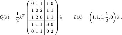
 satisfies


Then,

Alternative formulas for the colored Jones polynomial of 41 lead to identities among q-series. For instance, the Habiro formula for 41[30] combined with the above formula for  leads to the following identity:

The above identity has been proven by Armond-Dasbach. A detailed list of identities for knots with knots with at most 8 crossings is given in Appendix 14.
1.7 Extensions of stability
The methods that prove Theorem 1 are general and apply to several other circumstances of q-holonomic sequences that appear in quantum topology. We will list two results here.
Theorem 5.
If K is a positive link, then  is stable and the corresponding limit F
K
(x,q) is obtained by a Nahm sum associated to a positive downwards diagram of K. Moreover, for every
is stable and the corresponding limit F
K
(x,q) is obtained by a Nahm sum associated to a positive downwards diagram of K. Moreover, for every  we have
  .
.
The proof of the above theorem is easier than that of Theorem 1 since it does not require to center the states of the R-matrix state sum of a positive link. An example that illustrates the above theorem is taken from [31, Sec.1.1.4]: for the right-handed trefoil 31, its associated series is

Some results related to the zero stability of a class of positive knots are obtained in [32].
Next, we discuss an extension of Theorem 1 to evaluations of quantum spin networks. For a detailed discussion of those, we refer the reader to [33]-[35]. Using the notation of [35], let γ=(a,b,c,d,e,f) be an admissible coloring of the edges of the standard tetrahedron

Consider the standard spin network evaluation  [33, 35].
Theorem 6.
For every admissible γ, the sequence  is stable, and its limit is given by a Nahm sum.
For example, if γ=(2,2,2,2,2,2), then

and

where x=q n+1. In particular,

The proof of the above theorem follows easily from the fact that the quantum 6j-symbol is given by a one-dimensional sum of a q-proper hypergeometric summand, and the sum is already centered. The analytic and arithmetic properties of the corresponding Nahm sum will be discussed in forthcoming work [28, 29].
1.8 Plan of the proof
The strategy to prove Theorems 2 and 1 is the following:
We begin with the R-matrix state sum for the colored Jones polynomial, reviewed in Sections 2.2 to 2.4.
We center the downward diagram, its corresponding states and their weights in Section 4.1.
We factorize the weights of the centered states as the product of a monomial and an element of  in Section 4.1. The advantage of using centered states is that the lowest q-degree of their weights is the sum of a quadratic function Q(s) of s with a quadratic function of n.
Although Q(s) is not a positive definite quadratic form, in Section 5.3 we show that Q(s) is copositive on the cone of the centered states. The proof uses the combinatorics of alternating downward diagrams, and their centered states, reminiscent to the Kauffman bracket.
In Section 7, we prove the zero stability Theorem 2.
If Q(s) were positive definite, then it would be easy to deduce Theorem 1. Unfortunately, Q(s) is never positive definite, and it always has directions of linear growth in the cone of centered states. In Section 8, we state a partition of the set of k-bounded states, and prove stability away from the region of linear growth. Section 9 deals with stability in the region of linear growth.
Section 10 is rather technical, and gives a proof of the key Proposition 4.
Section 11 deduces the q-holonomicity of the sequence Φ K,k (q) of an alternating link from the q-holonomicity of the corresponding colored Jones polynomial. As a result, we obtain sharp quadratic lower bounds for the minimum degree of Φ K,k (q) and sharp bounds for the convergence of the colored Jones polynomial stated in Theorem 4.
In Section 12, we give an algorithm for computing Φ K,k (q) from a reduced alternating planar projection.
In Section 13, we prove that Φ K,0(q) is determined by the reduced Tait graph of an alternating link K.
In Section 14, we give some illustrations of Theorems 2 and 1.
1.9 Follow-up work
The topic of stability (affectionately called head/tail by Dasbach-Lin [36]) has recently attracted a lot of attention. After the papearance of our paper on the arxiv in the late 2011, a number of papers have since been posted. Among them, Hajij gives a skein-theory proof of zero stability for alternating links and some quantum spin networks [37, 38]. Motivated by the q-series of Nahm type, Andrews proves some Rogers-Ramanujan type identities [39]. Vuong and the first author give efficient algorithms to compute the zero limit of an alternating knot [40]. Vuong-Norin and the first author identify the coefficients of q k of the zero limit for k=0,…,3 in terms of graph countings of induced plane subgraphs of the reduced Tait graph of an alternating link [41]. Norin and the first author prove that each coefficient of q k in the zero limit is a polynomial of induced plane subgraphs of the reduced Tait graph of an alternating link [42]. Finally, in another direction, q-series of Nahm type were studied by Beem-Dimofte-Pasquetti and Kashaev and the first author; see [43, 44].
2 The R-matrix state-sum of the colored Jones polynomial
In this section, we review the R-matrix state sum of the colored Jones function, discussed in detail in [14, 15, 25]. We will use the following standard notation in q-calculus.

2.1 Downward link diagram
Recall that a link diagram  is alternating if walking along it, the sequence of crossings alternates from overcrossings to undercrossings. A diagram D is reduced if it is not of the form

where D 1 and D 2 are diagrams with at least one crossing.
A downward link diagrams of links is an oriented link diagram in the standard plane in general position (with its height function) such that at every crossing, the orientation of both strands of the link is downward. A usual link diagram may not satisfy the downward requirement on the orientation at a crossing. However, it is easy to convert a link diagram into a downward one by rotating the non-downward crossings as follows:

2.2 Link diagrams and states
Fix a downward link diagram D of an oriented link K with c D crossing. Considering D as a four-valent graph, it has 2c D edges. A state of D is a map

such that at every crossing, we have

where a,b,c,d are the values of s of the edges incident to the crossing as in the following equation

The set  of all states of D is a vector space. For a state
  and a crossing v of D define

where as usual the sign of the crossing on the left-hand side of (11) is positive and the sign of the one on the right-hand side is negative. For a positive integer n, a state  is called n-admissible if the values of r are integers in [ 0,n] and r(v)≥0 for every crossing v. Let S
D,n
be the set of all n-admissible states.
is called n-admissible if the values of r are integers in [ 0,n] and r(v)≥0 for every crossing v. Let S
D,n
be the set of all n-admissible states.
Remark 9
Later we will prove that  . By definition, S
D,n
in 1-1 correspondence with the set
. By definition, S
D,n
in 1-1 correspondence with the set  of lattice points of n
P
D
for a lattice polytope P
D
in
of lattice points of n
P
D
for a lattice polytope P
D
in  where c
D
is the number of crossings of D.
where c
D
is the number of crossings of D.
2.3 Winding number and its local weight
Suppose α is an oriented simple closed curve in the standard plane. By the winding number W(α), we mean the winding number of α with respect to a point in the region bounded by α. Observe that W(α)=1 if α is counterclockwise, −1 if otherwise.
The winding number W(α) can be calculated by a local weight sum as follows. A local part of α is a small neighborhood of a local maximum or minimum. For a local part X define W(X)=1/2 if X is winding counterclockwise, −1/2 if otherwise. In other words, we have

The next lemma is elementary.
Lemma 1
For every simple closed curve α,

where the sum is over all the local parts of α.
2.4 Local weights, the colored Jones polynomial, and their factorization
Consider the monoid

Fix a natural number n≥1 and a downward link diagram D.
A local part of D is a small neighborhood of a crossing or a local extreme of D. There are six types of local parts of D: two types of crossings (positive or negative) and four types of local extrema (minima or maxima, oriented clockwise, or counterclockwise):

For an n-admissible state r and a local part X, the weight w(X,r) is defined by

where  is a monomial,
  , and w
lt(X,r) and w
≻(X,r) are given by Table 1.
, and w
lt(X,r) and w
≻(X,r) are given by Table 1.
For a local extreme point X with the value of the state a, we have the convenient formula

Let the weight of a state be defined by

where the product is over all the local parts of D. Then the unframed version of the colored Jones polynomial of the link K, each component of which is colored by the n+1-dimensional s l 2-module, is given by

where S D,n is the set of all n-admissible states of D. For example, the value of the unknot is

Note that J K,0(q)=1 for all links and J K,1(q −1)/J Unknot,1(q −1) is the Jones polynomial of K[45]. Since we could not find a reference for the state sum formula (14) in the literature, we will give a proof in the Appendix.
3 Alternating link diagrams and centered states
In this section, we will discuss the combinatorics of alternating diagrams.
3.1 Alternating link diagrams and A-infinite type
Recall that a link diagram D gives rise to a polygonal complex structure of  , and if D is alternating and connected, then the checkerboard coloring with colors A and B at each crossing looks like Figure 1.
If K is non-split, then D is a connected graph. If K is split, then D has several connected components. We will say that an alternating diagram D is A-infinite if the point ∞∈S 2 is contained in an A-polygon of every connected subgraph of D. It is clear that by moving the connected components of D around in S 2, we can assume that D is A-infinite. This will make the colors of different connected components compatible.
We will use the following obvious property of an A-infinite alternating link diagram: all the B-polygons are finite, i.e. in  .
.
For example, the left-handed trefoil given by the standard closure of the braid  is A-infinite, whereas the right-handed trefoil given by the standard closure of the braid
  is not. Here s
1 is the standard generator of the braid group in two strands.
is not. Here s
1 is the standard generator of the braid group in two strands.
3.2 The digraph  of an alternating diagram D
 of an alternating diagram D
Let D be an oriented link diagram. Recall that we consider D also as a graph whose edges are oriented. We say that an edge of D is of type O if it begins as an overpass, and of type U if it begins as an underpass. If D is alternating and one travels along the the link, the edges alternate from type U to type O and vice-versa.
For a link diagram D, let  be the directed graph on
  obtained from the projection of D on the plane by reversing the orientation of all edges of type O. For example, a planar projection D and the corresponding digraph
  of the 41 knot is shown in Figure 3.

A planar projection
D
of the
4
1
knot on the left and the corresponding digraph
 on the right. If we checkerboard color the faces of
  with the unbounded one being white, then all black faces are oriented counter clockwise and all bounded white faces are oriented clockwise.
If D is downward alternating, it is easy to see that  is obtained from D by the following changing of orientations near a crossing point,

i.e., if the crossing is a positive one, then the two left edges incident to it get orientation reversed, and if the crossing is negative, then the two right edges incident to it get orientation reversed.
We will retain the markings A and B for angles and regions of complements of  .
.
At every vertex of  (or a crossing of D), there are two ways to smoothen the diagram. Following Kauffman [46] we call the A-smoothening (resp., B-smoothening) the one where the two A-regions (resp., B-regions) get connected. See the following equation for two examples of an A-smoothening.

Note that after either type of smoothening, the orientation of the edges of  is still well-defined.
Remark 10
Doing an A-resolution (resp. B-resolution) on a vertex of  is the same as doing an A-resolution (resp. B-resolution) on the original diagram D in the sense of Kauffman [47]. The advantage here, with directed graph
  for the case of alternating links, is that the resulting graph of any resolution is still oriented.
Part (b) of the following lemma is where A-infinity is used in an essential way.
Lemma 2
Suppose D is an alternating link diagram, (a) To the right of every oriented edge of  is an A-polygon, and to the left of every oriented edge of
  is a B-polygon. (b) Suppose D is A-infinite, then every circle obtained from
  by after doing A-resolution at every vertex of
  bounds a polygonal region of type B. Moreover, every such circle is winding counterclockwise, i.e., it has winding number 1. (c) If D is reduced, then each circle in (b) does not self-touch, i.e., the two arcs resulting from the A-resolution at one vertex do not belong to the same circle.
Proof
(a) This follows easily by inspecting the directions of the edges and the markings of the regions at the two types of vertices of  . (b) The boundaries of the B-polygons are exactly the circles obtained from D after doing A-resolution at every vertex of D. Since the infinity region is not a B-type region, every circle does bound a B-type region in the plane
  . From part (a), it follows that each circle, which is the boundary of a polygonal region of type B, is counterclockwise. (c) This is a well-known fact. A link diagram having the property that no circle obtained after doing A-resolution at every crossing has a self-touching point is known as an A-adequate diagram. In [17, Prop.5.3], it was proved that every reduced alternating link diagram is A-adequate.
3.3 Centered states
Fix an alternating downward diagram D with c
D
crossings and its directed graph  . Recall that
  and
and  denote respectively the set of oriented edges of
  and the set of vertices of
  .
.
A centered state of  is a map
  such that at every vertex v, we have

with the convention that a,b,c,d are the values of s as indicated in the following equation:

For the above vertex, we define

thus extending s to a map  .
.
Let  and
and  denote the sets of all centered states of
  with values respectively in
  and in
  . For a fixed positive integer n, define a map

by

It is easy to see that the map (19) is a vector space isomorphism. If r∈S
D,n
, i.e., r is n-admissible, then  is called n-admissible. Let
  be the set of all n-admissible centered states.
To characterize n-admissible centered states let us introduce the following norm for  :
:

The following is a reformulation of n-admissibility in terms of centered states.
Lemma 3
A centered state s is n-admissible if and only if  and |s|≤n. In other words,

Proof.
This follows immediately from the definition, since for any state r and for every vertex v of  we have
  .
.
It follows that if a centered state is n-admissible, then it is (n+1)-admissible.
4 Local weights in terms of centered states
In this section, we will give an explicit formula for the weight of a centered state. It turns out that the state sum of the colored Jones polynomial in terms of centered states has the important property of separation of variables needed in the proof of the stability. See Remark 12.
4.1 Local weights of centered states and their factorization
For an n-admissible centered state  , let us define w(s):=w(r). From the state sum of w(r), we get the following state sum for w(s):

where the sum is over all the local part X of  . Here, a local part of
  is a neighborhood of either a vertex or an extreme point of
  , and the value of

is obtained by replacing Table 1 with Table 2,
where

Note that w
≻(X,s) is independent of the sign of the local crossing and takes the same value 1 at all local extrema. Hence, we use the notation w
≻(v,s) for the right-hand side of (21), where  is the involved vertex. The following is a convenient way to rewrite the value of w
≻(v,s).
is the involved vertex. The following is a convenient way to rewrite the value of w
≻(v,s).
Lemma 4
For a vertex v in (17) and x=q n+1, we have

Proof.
The identity follows from Equation 21, and the following (easy to check) identities

Remark 11
The right-hand side of Equation 22 can also be written in the following form:

4.2 The functionals P 0,P 1,Q,L 0,L 1
To study the power of q in Table 2, let us introduce the following functionals P 0,P 1,Q,L 0,L 1 on centered states, defined by local weights as in Table 3.
If F is one of the functionals P 1,P 2,Q,L 0,L 1, and s is a centered state, then we define

where the sum is over all local parts X, with the value of F at a local part is given in Table 3. These functionals are introduced so that for a local part X with centered state s, we have

From Equation 20, we have

Here  , where the product is over all local parts of D. Note that
  . The functionals L
0,L
1 are linear forms on
. The functionals L
0,L
1 are linear forms on  and do not depend on n in the sense that the value of each of L
0,L
1 will be the same if we consider s as an (n+1)-admissible centered state instead of an n-state. The functional Q
2=Q+L
1 is a quadratic form on
and do not depend on n in the sense that the value of each of L
0,L
1 will be the same if we consider s as an (n+1)-admissible centered state instead of an n-state. The functional Q
2=Q+L
1 is a quadratic form on  not depending on n. The two functionals P
0,P
1 depend only on n, i.e., if s,s
′ are n-admissible centered states, then P
i
(s)=P
i
(s
′). Hence, we will also write P
i
(n) instead of P
i
(s), for i=0,1.
not depending on n. The two functionals P
0,P
1 depend only on n, i.e., if s,s
′ are n-admissible centered states, then P
i
(s)=P
i
(s
′). Hence, we will also write P
i
(n) instead of P
i
(s), for i=0,1.
Lemma 5
We have

where

Proof.
By (22) we have

Here a and b (respectively c and d) are the s-values of the two lower (respectively upper) edges incident to v. When v runs the set  of vertices, the two lower edges of v run the set
  of all edges, as do the two upper edges of v. Hence,

From Equation 24 and  , we have

which is equal to the right hand side of (25) by identity (27) and the definition of F(x,q,s).
Remark 12
(a) It is important for the stability that there is no mixing between n and s in the formulas of the functionals P
0,P
1,Q,L
0,L
1. In the states-sum using states in D, mixing occurs, and this is the reason why we introduce centered states. (b) The quadratic form Q has the following simple description. Suppose α is an A-angle of the digraph  , and the s-values of the two edges of α are a and b. Define Q(α,s)=a
b/2. Then
, and the s-values of the two edges of α are a and b. Define Q(α,s)=a
b/2. Then

where the sum is over all A-angles α.
5 Positivity of Q 2and the lowest degree of the colored Jones polynomial
In this section, we prove the copositivity of Q
2:=Q+L
1 on the cone  and derive a formula for the lowest degree of the colored Jones polynomial. As before, we fix a reduced, alternating A-infinite downward diagram D with c
D
crossings.
and derive a formula for the lowest degree of the colored Jones polynomial. As before, we fix a reduced, alternating A-infinite downward diagram D with c
D
crossings.
5.1 A Hilbert basis for  : elementary centered states
 : elementary centered states
From its very definition, the set  of
of  -valued centered states of
  can be identified with the set of lattice points of a lattice cone in
  . In general, the set of lattice points of a rational cone is a monoid, and a generating set is called a Hilbert basis which plays an important role in integer programming; see for instance [48, Sec.13] and also [49, Sec.16.4]. Note that every element of a finitely generated additive monoid is an
  -linear combination of a Hilbert basis. Although the natural number coefficients are not unique, this is not a problem for applications.
The goal of this section is to describe a useful Hilbert basis for  .
.
Recall that  is a directed graph. Suppose γ is a directed cycle of
  , i.e., closed path consisting of a sequence of distinct edges e
1,…,e
n
of D such that the ending point of e
j
is the starting points of e
j+1 (index is taken modulo n) and there is no repeated vertex along the path except for the obvious case where the first vertex is also the last vertex. An example of a cycle of
, i.e., closed path consisting of a sequence of distinct edges e
1,…,e
n
of D such that the ending point of e
j
is the starting points of e
j+1 (index is taken modulo n) and there is no repeated vertex along the path except for the obvious case where the first vertex is also the last vertex. An example of a cycle of  is the boundary of a polygon in the complement of
  .
.
Definition 3
For a directed cycle γ of  , let s
γ
be the function on the set of edges of
, let s
γ
be the function on the set of edges of  which assigns 1 to every edge of γ and 0 to every other edge. Such a centered state is called elementary, and γ is called its support. Let
  denote the (finite set) of all elementary centered states of
  .
.
For a polygon  , the boundary ∂
p is a directed cycle of
, the boundary ∂
p is a directed cycle of  , and we will use the notation s
p
:=s
∂
p
.
, and we will use the notation s
p
:=s
∂
p
.
From Lemma 3, we see that s γ is an n-admissible centered state for every n≥1.
Lemma 6
 is a Hilbert basis of
  .
.
Proof.
Let s be an  -valued centered state of
  . Suppose e is an oriented edge such that s(e)>0. At the ending vertex v of e let e
′ and e
″ be the two edges which are perpendicular to e. Inspection of Equation 15 shows that v is the starting vertex for both e
′ and e
″. Equation 16 shows that s(e
′)+s(e
″)≥s(e). Hence one of them, say s(e
′)>0. This means if e is an edge with s(e)>0, we can continue e to another edge e
′ for which s(e
′)>0. Repeating this process, we can construct a cycle γ of
. Suppose e is an oriented edge such that s(e)>0. At the ending vertex v of e let e
′ and e
″ be the two edges which are perpendicular to e. Inspection of Equation 15 shows that v is the starting vertex for both e
′ and e
″. Equation 16 shows that s(e
′)+s(e
″)≥s(e). Hence one of them, say s(e
′)>0. This means if e is an edge with s(e)>0, we can continue e to another edge e
′ for which s(e
′)>0. Repeating this process, we can construct a cycle γ of  such that the value of s is positive on any edge of γ. This means s−s
γ
is an
such that the value of s is positive on any edge of γ. This means s−s
γ
is an  -valued centered state. Induction completes the proof of the lemma.
Remark 13
It is easy to see that any  is not a
  -linear combination of the other elements in
  . Thus there is no redundant element in
  . Of course
  is linearly dependent over
  (or over
  ), and we will extract a
  -basis from the set
  later.
5.2 Values of L 1and Qon elementary centered states
Suppose γ is a directed cycle of  and v is a vertex of γ. Among the four edges of
  incident to v, the two edges of γ are not two opposite edges because of the orientation constraint, see (15). In other words, at each vertex v, γ is an angle. We say that a vertex v of γ is of type A or B according as the two edges of γ at v form an angle of type A or B. Let N
γ,A
be the number of vertices of γ of type A. The fact that D is reduced is used in the proof of part (b) of the next lemma.
incident to v, the two edges of γ are not two opposite edges because of the orientation constraint, see (15). In other words, at each vertex v, γ is an angle. We say that a vertex v of γ is of type A or B according as the two edges of γ at v form an angle of type A or B. Let N
γ,A
be the number of vertices of γ of type A. The fact that D is reduced is used in the proof of part (b) of the next lemma.
Lemma 7
Suppose  is an elementary centered state.
-
(a)
We have
 (29)
(29) -
(b)
Moreover, L 1(s)≥0, and L 1(s)=0 if and only if γ is clockwise and has exactly two vertices of type A.

Proof.
-
(a)
For a local part X of
 , let γ
X
=γ∩X. Clearly L
1(X,s)=0 if γ
X
=∅. If X is a small neighborhood of a vertex of
, let γ
X
=γ∩X. Clearly L
1(X,s)=0 if γ
X
=∅. If X is a small neighborhood of a vertex of  , then γ
X
is two sides of an angle of γ, and we will smoothen γ
X
at the corner to get an oriented smoothed arc. See row 1 and row 2 of Table 4 for various X and smoothened γ
X
. In the table, X is a small neighborhood of a vextex. The two edges incident to the vertex with label 1 belong to γ. The marking A or B at one of the angles of X indicates the type of the vertex, which appear in row 3. In row 3, we also indicate the sign of the crossing of X (as it appeared originally in D); this makes the computation of L
1 easier.
, then γ
X
is two sides of an angle of γ, and we will smoothen γ
X
at the corner to get an oriented smoothed arc. See row 1 and row 2 of Table 4 for various X and smoothened γ
X
. In the table, X is a small neighborhood of a vextex. The two edges incident to the vertex with label 1 belong to γ. The marking A or B at one of the angles of X indicates the type of the vertex, which appear in row 3. In row 3, we also indicate the sign of the crossing of X (as it appeared originally in D); this makes the computation of L
1 easier.
 , let γ
X
=γ∩X. Clearly L
1(X,s)=0 if γ
X
=∅. If X is a small neighborhood of a vertex of
, let γ
X
=γ∩X. Clearly L
1(X,s)=0 if γ
X
=∅. If X is a small neighborhood of a vertex of  , then γ
X
is two sides of an angle of γ, and we will smoothen γ
X
at the corner to get an oriented smoothed arc. See row 1 and row 2 of Table
, then γ
X
is two sides of an angle of γ, and we will smoothen γ
X
at the corner to get an oriented smoothed arc. See row 1 and row 2 of Table We define W(γ
X
) to be its local winding number if γ
X
contains a local extreme point, 0 otherwise. Rows 4 and 5 of Table 4 gives the values of L
1(X,s
γ
) and W(γ
X
). From the table, together with the obvious case when X is a neighborhood of a local extreme point of  , we have

Summing up the above identity over all the local parts X and using (12), we get (29).
-
(b)
Case 1: γ is counterclockwise. From (29), we have L 1(s)≥W(γ)=1>0. In this case L 1 is strictly positive.
Case 2: γ is clockwise. Then L 1(s)=−1+N γ,A /2. We will show that N γ,A ≥2.
If N
γ,A
=0, then γ is one of the circles obtained from  by doing A-resolution at every vertex. By part (b) of Lemma 2, γ is counterclockwise. Thus, N
γ,A
≠0 if γ is clockwise.
by doing A-resolution at every vertex. By part (b) of Lemma 2, γ is counterclockwise. Thus, N
γ,A
≠0 if γ is clockwise.
Suppose N
γ,A
=1, i.e. γ has exactly one vertex of type A, say v; all other vertices of γ are of type B. If one does A-resolution at every vertex of  , then γ∖{v} is part of one of the resulting circles, and this circle has a self-touching point at v. This is impossible if the diagram D is reduced, see part (c) of Lemma 2. Thus, N
γ,A
≠1.
, then γ∖{v} is part of one of the resulting circles, and this circle has a self-touching point at v. This is impossible if the diagram D is reduced, see part (c) of Lemma 2. Thus, N
γ,A
≠1.
We have shown that if γ is clockwise then N γ,A ≥2. Hence, L 1(s)=−1+N γ,A /2≥0, and equality happens if and only N γ,A =2.
Remark 14
We see that for the proof of part (b), we need only the fact that D is A-adequate.
Lemma 8
-
(a)
For all
 -valued centered states s and s
′, we have
-valued centered states s and s
′, we have  (30)
(30) -
(b)
Suppose
 is elementary centered state. Then
  (31)
(31)
 -valued centered states s and s
′, we have
-valued centered states s and s
′, we have 
 is elementary centered state. Then
It follows that Q(s)≥0, with equality if and only if γ is the boundary of a polygonal region of type B.
Proof.
-
(a)
Since Q is defined by an expression with positive coefficients, we have Q(s+s ′)≥Q(s)+Q(s ′). (b) Row 6 of Table 4 shows that every vertex of type A of γ contributes 1/2 to the value of Q, while others contribute 0. Hence,


5.3 Copositivity of Q 2
Recall that Q 2=Q+L 1.
Proposition 1
-
(a)
For
 , we have
-
(b)
If
 , where
  and
and  , then
  (32)
(32)
 , we have
 , where
  and
and  , then
In particular, Q
2 is copositive in the cone  , i.e., for every
  , Q
2(s)≥0 and equality happens if and if only s=0.
, Q
2(s)≥0 and equality happens if and if only s=0.
Proof.
-
(a)
This follows immediately from Lemma 8(a), noting that L 1(s+s ′)=L 1(s)+L 1(s ′). (b) The second inequality of (32) follows immediately from the definition.
From part (a), one needs only to prove the first inequality of (32) for  , an elementary centered state with support γ. By (29) and (31),

In particular, Q
2(s) is an integer. By Lemmas 7(b) and 8(b), we have L
1(s)+Q(s)≥0, and equality happens only when L
1(s)=Q(s)=0. However, if L
1(s)=0, then by Lemma 7(b), N
γ,A
=2, and then Q(s)=N
γ,A
/2=1>0. Thus, we have proved that if s is an elementary centered state, then Q(s)>0. Since  , we have Q(s)≥1.
Remark 15
In general,  . In the proof, we show that
  for any elementary centered state s. One can also show that
  for all
  . This can be deduced from the fact that
  , see the discussion on fractional powers of J
K,n
in [18].
, see the discussion on fractional powers of J
K,n
in [18].
5.4 The lowest degree of the colored Jones polynomial
In the next proposition K is an alternating link.
Proposition 2
-
(a)
The minimal degree of q in of J K,n (q) is


where the last sum is over all the local extreme points of D.
-
(b)
With F(x,q,s) defined by (26), we have
 (33)
(33)

Proof.
-
(a)
By (25), the minimal degree of q in w(s) is P 1(n)+Q 2(s). When s≠0, Proposition 1 implies that Q 2(s)>0. Hence the smallest degree of J K,n (q) is P 1(n). From the values of P 1(X,s) in Table 3 we see that
 . (b) follows easily from part (a) and (27).
 . (b) follows easily from part (a) and (27).
The value of P 0 in Table 4, Equation 25, and Proposition 2 imply the following:
Corollary 3
We have

Remark 16
The minimal degree of the colored Jones polynomial J
K,n
(q) of an alternating link had been calculated using the Kauffman bracket skein module, and is given by  , where s
A
is the number of circles obtained from
, where s
A
is the number of circles obtained from  by doing A-resolution at every vertex; see [16, Proposition 2.1] and keep in mind that the framing of K in [16] is different from the one in the current paper. Our result implies that P
1(n)=P1′(n). We will give a direct proof of this identity in the Appendix. Note also that s
A
−c
+=σ+1 (see [19, 50]), where σ is the signature of the link. Hence the lowest degree of q is given by
by doing A-resolution at every vertex; see [16, Proposition 2.1] and keep in mind that the framing of K in [16] is different from the one in the current paper. Our result implies that P
1(n)=P1′(n). We will give a direct proof of this identity in the Appendix. Note also that s
A
−c
+=σ+1 (see [19, 50]), where σ is the signature of the link. Hence the lowest degree of q is given by  .
.
6 From  to the dual graph D
∗
to the dual graph D
∗
 to the dual graph D
∗
to the dual graph D
∗
In this section, we give a correspondence between the centered states on  with the admissible colorings of the dual graph D
∗. The main idea is summarized in Figure 4. If a crossing has coloring a,b,c,d at the four regions of it counterclockwise, then there is a coloring of the four arcs such that the sum of the colors of the two overarcs is equal to the sum of the colors of the two underarcs:
with the admissible colorings of the dual graph D
∗. The main idea is summarized in Figure 4. If a crossing has coloring a,b,c,d at the four regions of it counterclockwise, then there is a coloring of the four arcs such that the sum of the colors of the two overarcs is equal to the sum of the colors of the two underarcs:

From a coloring of the regions to a coloring of the arcs.
An example of this correspondence for the 41 knot is shown in Figure 5.

Admissible coloring of
D
∗
, coloring polygons of
D
and corresponding centered state on
 for
4
1
knot.
for
4
1
knot.
Recall from Section 1.4 that D
∗ is the dual graph of  , considered as an unoriented graph. We have defined the Tait graph
  , the lattice Λ
0 with its subsets Adm, Adm(n), and functions L,Q on Λ
0. Note that one does not need to bring D to a downward position by twisting in small neighborhood of crossing points in order to construct D
∗.
, the lattice Λ
0 with its subsets Adm, Adm(n), and functions L,Q on Λ
0. Note that one does not need to bring D to a downward position by twisting in small neighborhood of crossing points in order to construct D
∗.
For λ∈Λ
0, let  be the linear map defined by

where  is the dual edge of e. Then
  is a
is a  -linear map.
Proposition 3
-
(a)
The map
 is vector space isomorphism. (b) τ maps Adm and Adm(n) isomorphically onto respectively
  and
and  . (c) We have
  (35)
(35) (36)
(36) -
(d)
For every centered state s, we have
 (37)
(37)
 is vector space isomorphism. (b) τ maps Adm and Adm(n) isomorphically onto respectively
  and
and  . (c) We have


Proof.
-
(a)
Fix
 . We will show that the equation
  (38)
(38)
 . We will show that the equation
has one and exactly one solution λ∈Λ 0. This will prove the bijectivity of τ.
With the basis  of Λ
0, every λ∈Λ
0 has a unique presentation
of Λ
0, every λ∈Λ
0 has a unique presentation  with k
v
=0 for v=v
∞
. We need to solve for k
v
,v∈b from Eq. 38.
with k
v
=0 for v=v
∞
. We need to solve for k
v
,v∈b from Eq. 38.
Eq. 38 is the same as the following linear system of 2c
D
equations: For every edge  whose end points are v and v
′,
whose end points are v and v
′,

If k
v
is known, and v
′ is connected to v by an edge, then there is only one possible value for  , namely
  . We call such
  the extension of the value k
v
at v along the edge e
∗. Since the graph D
∗ is connected, and
the extension of the value k
v
at v along the edge e
∗. Since the graph D
∗ is connected, and  , we see that there is at most one solution λ∈Λ
0 of (38).
, we see that there is at most one solution λ∈Λ
0 of (38).
Now let us look at the existence of solution of (38). Given  ,
,  , and a path α of the graph Δ
∗ connecting v to
, and a path α of the graph Δ
∗ connecting v to  , there is only one way to extend k
v
=a at v to v
′ along the path α. Denote by λ
α,a
(v
′) the value at v
′ of this extension. When α is a closed path, i.e. v
′=v, let Δ(α,a)=λ
α,a
(v
′)−a. We will show that Δ(α,a)=0 for any closed path α. This will prove the existence of the solution.
, there is only one way to extend k
v
=a at v to v
′ along the path α. Denote by λ
α,a
(v
′) the value at v
′ of this extension. When α is a closed path, i.e. v
′=v, let Δ(α,a)=λ
α,a
(v
′)−a. We will show that Δ(α,a)=0 for any closed path α. This will prove the existence of the solution.
On  , the closed path α encloses a region R. When the region is just a polygon of D
∗ (which must be a quadrilateral), the fact that Δ(α,a)=0 follows easily from (16). For general closed path α, since Δ(α,a) is the sum of
, the closed path α encloses a region R. When the region is just a polygon of D
∗ (which must be a quadrilateral), the fact that Δ(α,a)=0 follows easily from (16). For general closed path α, since Δ(α,a) is the sum of  , where α
j
’s are the boundaries of all the polygons of D
∗ in R, we also have Δ(α,a)=0.
, where α
j
’s are the boundaries of all the polygons of D
∗ in R, we also have Δ(α,a)=0.
The above fact shows that if we begin with  , we can uniquely extend k
v
to all vertices of D
∗, and obtain in this way an inverse of s.
, we can uniquely extend k
v
to all vertices of D
∗, and obtain in this way an inverse of s.
The proof actually shows that τ is a  -isomorphism between Λ
0 and
-isomorphism between Λ
0 and  .
.
-
(b)
Because τ(λ)(e)=λ(e ∗), (b) follows easily from the definitions.
-
(c)
To prove (35), it is enough to consider the case
 , a basis vector. Let
  be the dual polygon. From the definition we have τ(v)=s
p
, where s
p
is the elementary centered state with support being the boundary of p. Now the identity L
1(τ(v))=L(v) follows from the value of L
1 given in Lemma 7 and the definition of L. Actually, the definition of L was built so that (35) holds.
be the dual polygon. From the definition we have τ(v)=s
p
, where s
p
is the elementary centered state with support being the boundary of p. Now the identity L
1(τ(v))=L(v) follows from the value of L
1 given in Lemma 7 and the definition of L. Actually, the definition of L was built so that (35) holds.
 , a basis vector. Let
  be the dual polygon. From the definition we have τ(v)=s
p
, where s
p
is the elementary centered state with support being the boundary of p. Now the identity L
1(τ(v))=L(v) follows from the value of L
1 given in Lemma 7 and the definition of L. Actually, the definition of L was built so that (35) holds.
be the dual polygon. From the definition we have τ(v)=s
p
, where s
p
is the elementary centered state with support being the boundary of p. Now the identity L
1(τ(v))=L(v) follows from the value of L
1 given in Lemma 7 and the definition of L. Actually, the definition of L was built so that (35) holds.Let us turn to (36). To show that two quadratic forms on a vector space are the same it is enough to show that they agree on the set v+v
′, where v,v
′ are elements in a basis of the vector space. A basis of Λ
0 is  . Hence, we need to check that if
  ,
,

There are three cases to consider: both v
1,v
2 are A-vertices, both are B-vertices, and exactly one of them is an A-vertex. In each case, the identity (40) can be verified easily. Actually, the matrix  in Equation 4 was defined so that Equation 40 holds.
-
(d)
We only need to check (37) for s=τ(v),v∈b. Let
 be the dual polygon. We already saw that τ(v)=s
p
. From the definition of L
0 given by Table 3, we have that L
0(s
p
) is the number of negative vertices of p. Here a vertex is negative if it is negative as a crossing of the link diagram D.
be the dual polygon. We already saw that τ(v)=s
p
. From the definition of L
0 given by Table 3, we have that L
0(s
p
) is the number of negative vertices of p. Here a vertex is negative if it is negative as a crossing of the link diagram D.
 be the dual polygon. We already saw that τ(v)=s
p
. From the definition of L
0 given by Table
be the dual polygon. We already saw that τ(v)=s
p
. From the definition of L
0 given by Table There are two cases:
Case 1: p is a B-polygon. Suppose or is an arbitrary orientation on edges of p. A vertex v of p is or-incompatible if the orientations of the two edges incident to v are incompatible, i.e. the two incident edges are both going out from v or both coming in to v. Let f(or) be the number of all or-incompatible vertices. It is easy to see that if or′ is obtained from or by changing the orientation at exactly one edge, then f(or)=f(or′) (mod 2). It follows that f(or)=0 (mod 2) for any orientation or, since if we orient all the edges counterclockwise then f=0.
Let the orientation of D on the edges of p be denoted by or D . By inspection of Equation 15 one sees that a vertex v of p is a negative crossing if and only if v is or D -incompatible. Thus, L 0(s p )=f(or D ), which is even by the above argument. On the other hand, 2L 1(s p )=2 by Lemma 7.
Case 2: p is an A-polygon. By inspection of Equation 15, one sees that a vertex v of p is a positive crossing if and only if v is or D -incompatible. This means L 0(s p )= deg(v)−f(or D )≡ deg(v) (mod 2), where deg(v) is the number of vertices of p, which is equal to the degree of v in the graph D ∗. By Lemma 7, 2L 1(s p )=−2+ deg(v). Hence, we also have (37).
Example 1
As an illustration of Equation 36, consider the coloring on D
∗ and the corresponding state on  from Figure 5. We have

The reader can vefiry the equality (36).
Corollary 4
The dimension of  (or
(or  ) is c
D
+ℓ, where ℓ is the number of connected components of the graph D.
) is c
D
+ℓ, where ℓ is the number of connected components of the graph D.
Remark 17
One can show that the integer-valued admissible colorings of D ∗ are the lattice points in a 2c D dimensional cone with 2c D independent rays.
7 Zero stability
In this section, we give a proof of the zero stability of the colored Jones polynomial of an alternating link and Theorem 2, which describes the zero limit as a generalized Nahm sum.
7.1 Expansion of Fand adequate series
Definition 4
We say that a series  is x-adequate of order ≤t if
  , i.e. for every m, we have

Lemma 9
-
(a)
For every
 , the set of x-adequate series of order ≤t is a subring of
  . (b) If G(x,q) is x-adequate of order ≤t, then it is x-adequate of order ≤t
′ for any t
′≥t. (c) If G(x,q) is x-adequate of order ≤t, then the series f
n
(q)=G(q
n,q) converges in the q-adic topology and defines an element in
. (b) If G(x,q) is x-adequate of order ≤t, then it is x-adequate of order ≤t
′ for any t
′≥t. (c) If G(x,q) is x-adequate of order ≤t, then the series f
n
(q)=G(q
n,q) converges in the q-adic topology and defines an element in  for every n>t. (d) The sequence in (c) is stable and its associated series F
f
(x,q) satisfies F
f
(x,q)=G(x,q).
for every n>t. (d) The sequence in (c) is stable and its associated series F
f
(x,q) satisfies F
f
(x,q)=G(x,q).
 , the set of x-adequate series of order ≤t is a subring of
  . (b) If G(x,q) is x-adequate of order ≤t, then it is x-adequate of order ≤t
′ for any t
′≥t. (c) If G(x,q) is x-adequate of order ≤t, then the series f
n
(q)=G(q
n,q) converges in the q-adic topology and defines an element in
. (b) If G(x,q) is x-adequate of order ≤t, then it is x-adequate of order ≤t
′ for any t
′≥t. (c) If G(x,q) is x-adequate of order ≤t, then the series f
n
(q)=G(q
n,q) converges in the q-adic topology and defines an element in  for every n>t. (d) The sequence in (c) is stable and its associated series F
f
(x,q) satisfies F
f
(x,q)=G(x,q).
for every n>t. (d) The sequence in (c) is stable and its associated series F
f
(x,q) satisfies F
f
(x,q)=G(x,q).Proof.
Parts (a), (b) and (c) follow easily from the definition of an x-adequate series.
For (d), let  and define Φ
k
(q)=a
k
(q) for all
and define Φ
k
(q)=a
k
(q) for all  . Then, we have for n>t+1

The minimum degree of the summand is bounded below by

Since f(m) is a linear function of m and the coefficient of m in f(m) is n+1−t>0, it follows that

Thus,

which implies (d).
Recall that for a centered state s, F(x,q,s) defined by (26), satisfies

Using the well-known identities (see e.g [51])

we can expand  into power series in x,

The negative powers of q in a
m
(q,s) come from the negative powers q
−s(v),q
−s(e) that appear in the expression of  . Since |s|≥ max(s(v),s(e)), we have the following:
Lemma 10
For every  ,
,  is x-adequate of order ≤|s|.
7.2 Proof of zero stability
Now we show that  is zero stable, and identify its zero limit. Recall F(x,q,s) given by (26) or (41). By (33)

Hence we expect that the zero limit is

We have

Part (b) of Proposition 1 shows that the right-hand side of (44) is regular, and defines an element in  . We will show that

for all n. This certainly implies that the zero limit of  exists and is equal to Φ
0(q). We have
exists and is equal to Φ
0(q). We have

By part (b) of Proposition 1, Q
2(s)≥|s|. Then (45) implies that  , and hence, the second sum on the right-hand side of (47) is in
  .
.
Let us look at the first term. Using the expansion (43), we have

where f(m)=Q 2(s)+m(n+1)−m|s|=m(n+1−|s|)+Q 2(s), which is linear in m. Since n≥|s|, f(m) achieves minimum when m=1:

By Lemma 10, a
m
(q,s) q
m|s| has only non-negative powers of q. It follows that the right-hand side of (48) belongs to  . This completes the proof of Equation 46. □
Remark 18
Equation 46 is stronger than zero stability, and implies that for every  , the coefficient of q
m in
, the coefficient of q
m in  is independent of n for all n>m.
7.3 End of the proof of Theorem 2
To complete the proof of Theorem 2, it remains to prove that the right-hand side of (44) is equal to that of (5). This follows from Proposition 3. □
Remark 19
The fact that D is reduced is used only in the proof of Lemma 7. As seen in Remark 14, Lemma 7 holds if D is A-adequate; hence, Theorem 2 holds if D is not necessarily reduced, but A-adequate.
7.4 Proof of Corollary 1
Fix a complex number q with |q|=a<1. We only need to show that the sum on the right-hand side of (44) is absolutely convergent.
Choose 0<ϵ<1−a such that

This is possible by continuity since if ϵ=1−a, the right-hand side of the above inequality is 1 and a<1. Since  , it follows that |1−q
j|>a+ϵ for j big enough. Thus, there is constant C
1>0 such that for every n,
, it follows that |1−q
j|>a+ϵ for j big enough. Thus, there is constant C
1>0 such that for every n,

Since Q
2(s)≥|s|≥s(e) for every  , we have

We have

Thus,

where g(m) is the number of  such that Q
2(s)=m. Because Q
2(s) is quadratic and co-positive in
such that Q
2(s)=m. Because Q
2(s) is quadratic and co-positive in  , g(m) is bounded above by a quadratic function of m for large enough m. From Equation 49, it follows that the right-hand side of (52) is absolutely convergent. This completes the proof of Corollary 1.
8 Linearly bounded states
In this section, we will introduce a partition of the set of linearly bounded centered states, which will be key to the k-stability of the colored Jones polynomial. Throughout this section, we fix a reduced, alternating, A-infinite downward alternating link diagram D with c
D
crossings. Let  . Recall that for a polygon
  , s
p
is the elementary centered state which support the boundary of p.
, s
p
is the elementary centered state which support the boundary of p.
If  were positive definite, it would be easy to prove the stability of
  . Unfortunately, Q is not positive definite, and the summation cone
  always contains directions where Q
2(s)=Q(s)+L
1(s) grows linearly, and not quadratically. For instance, if p is a B-polygon, then Q
2(n
s
p
)=n is a linear function of n.
always contains directions where Q
2(s)=Q(s)+L
1(s) grows linearly, and not quadratically. For instance, if p is a B-polygon, then Q
2(n
s
p
)=n is a linear function of n.
Definition 5
We say that a centered state  is k-bounded for a natural number k if

For a subset  let
let  denote the set of k-bounded centered states in
  .
.
8.1 Balanced states at B-polygons
Suppose e is an edge of a B-polygon p. In this section, we always use the orientation on e coming from the directed graph  . The orientation of e is counterclockwise with respect to the interior of p. Incident to the ending vertex of e are four edges of
  , and let
  be the one opposite to e, i.e. in a small neighborhood of the vertex,
  looks like a cross, and e and
  are on a line as in the following figure:

Suppose  is a centered state. Recall that s is a function on the set of edges of
  and that we already extended s to the vertices of
  ; see Equation 18. Now we further extend s to the set of B-polygons of
  . Suppose p is a B-polygon of
  . Let
. Let

Definition 6
We will say that a state  is balanced at a B-polygon p if s(v)≤s(p) for every vertex v of p, and equality holds for at least one vertex.
8.2 Seeds
In this section, we introduce seeds, their partial ordering, and relative seeds.
We say that two B-polygons are disjoint if they do not have a common vertex. Suppose Π is a collection of disjoint B-polygons. Let nbd(Π) be the set of all edges of  incident to a vertex of a polygon in Π. Observe that every edge of a polygon in Π is in nbd(Π).
Definition 7
-
(a)
A seed θ=(Π,σ) consists of a collection Π of disjoint B-polygons and a map
 such that σ can be extended to a centered state
  which is balanced at every polygon in Π. Such s is called an extension of σ, and the set of all extensions of σ is denoted by
  . If σ is a seed and s an extension of it, then for all polygons p in Π and vertices v of p we can define σ(v)=s(v) and σ(p)=s(p) independent of s. In particular, σ is balanced at all polygons of Π. (b) The B-norm | |θ| |
B
of θ is the number of B-polygons in Π.
. If σ is a seed and s an extension of it, then for all polygons p in Π and vertices v of p we can define σ(v)=s(v) and σ(p)=s(p) independent of s. In particular, σ is balanced at all polygons of Π. (b) The B-norm | |θ| |
B
of θ is the number of B-polygons in Π.
 such that σ can be extended to a centered state
  which is balanced at every polygon in Π. Such s is called an extension of σ, and the set of all extensions of σ is denoted by
  . If σ is a seed and s an extension of it, then for all polygons p in Π and vertices v of p we can define σ(v)=s(v) and σ(p)=s(p) independent of s. In particular, σ is balanced at all polygons of Π. (b) The B-norm | |θ| |
B
of θ is the number of B-polygons in Π.
. If σ is a seed and s an extension of it, then for all polygons p in Π and vertices v of p we can define σ(v)=s(v) and σ(p)=s(p) independent of s. In particular, σ is balanced at all polygons of Π. (b) The B-norm | |θ| |
B
of θ is the number of B-polygons in Π.Note that for the empty seed θ=∅, we have  . Next, we define a partial order on the set of seeds.
Definition 8
Suppose θ=(Π,σ) and θ ′=(Π ′,σ ′) are seeds. Then θ≤θ ′ if Π⊂Π ′ and σ is the restriction of σ ′. We write θ<θ ′ if θ≤θ ′ and θ≠θ ′.
Observe that ∅≤θ for any seed θ. Moreover, if θ<θ ′, then | |θ| | B <| |θ ′| | B . Since the number of B-polygons is finite, we have the following simple but important fact:
Lemma 11
Every strictly increasing sequence of seeds is finite.
We now introduce relative seeds.
Definition 9
Suppose θ=(Π,σ) and θ
′=(Π
′,σ
′) are seeds with θ<θ
′. (a) Let  , where the last equality follows from the fact that seeds are balanced. (b) Let
  be the set of all
  of the form

where

8.3 A partition of the set of k-bounded states
In this section, we give a partition of the set of k-bounded states  and more generally, the set
  of k-bounded states with seed θ. The next proposition will be proven in Section 10.
Proposition 4
For every non-negative integer k and every seed θ there exists a constant C>0 such that if |s|>C
k
2 and  , then
  for a unique seed θ
′>θ with |θ
′∖θ|<k. In other words, up to elements s with |s|≤C
k
2, we have the following finite partition of the set
for a unique seed θ
′>θ with |θ
′∖θ|<k. In other words, up to elements s with |s|≤C
k
2, we have the following finite partition of the set  of k-bounded states:

Example 2
Observe that if θ=∅ and |θ ′|<1 then σ=0. Proposition 4 implies that if s is a one-bounded state of sufficiently large |s|, then

where m=|s|>|s ′|, P is a B-polygon and the support of s ′ is disjoint from P.
On the other hand, if |θ ′|=1 then the restriction of σ on P looks like Figure 6. In other words, the support of σ is an incoming edge of P, followed by a counterclockwise path along P and finally by an outgoing edge of P. Proposition 4 implies that if s is a two-bounded state of sufficiently large |s|, then either

where m=|s|>|s ′|, P 1,P 2 are disjoint B-polygon and the support of s ′ is disjoint from P 1∪P 2, or

where m=|s|>|s ′|, P is a B-polygon as in Figure 6 and s ′ is balanced on P.

A seed θ ′ with |θ ′ |=1 .
When θ is maximal, Proposition 4 implies the following:
Corollary 5
For every non-negative integer k and every maximal seed θ,  is a finite set.
The next proposition will also be proven in Section 10.
Proposition 5
-
(a)
Suppose
 with presentation (54) as in Definition 9. One has |s|=m and
  (56)
(56) (57)
(57) -
(b)
Fixing θ<θ ′, the presentation of
 given by Equation 54, with (m,s
′) satisfying (55) is unique. In other words, the map (m,s
′)↦s given by (54) is a bijection between the set of pairs (m,s
′) satisfying (55) and
given by Equation 54, with (m,s
′) satisfying (55) is unique. In other words, the map (m,s
′)↦s given by (54) is a bijection between the set of pairs (m,s
′) satisfying (55) and  .
.
 with presentation (54) as in Definition 9. One has |s|=m and

 given by Equation
  .
.8.4 The weight of k-bounded states
In this section, we express F(x,q,s) in terms of F(x,q,s ′) for centered states s,s ′ related by Equation 54.
Definition 10
We say that a series  is weakly x-adequate of order less ≤t if
  for some constant C depending on G, i.e.

for every i,j≥0.
The next lemma is elementary.
Lemma 12
-
(a)
If G(x,y,q) is weakly x-adequate of order ≤t, then
 for every k≥t+1, l≥0. (b) If
  is weakly x-adequate of order ≤t, then for every
  ,
,  is x-adequate of order t. (c) The set of weakly x-adequate series of order less ≤t is closed under addition and multiplication, i.e. it is a
  -subalgebra of
  . (d) If G(x,y,q) is weakly x-adequate of order ≤t, then it is weakly x-adequate of order ≤t
′ for every t
′≥t.
. (d) If G(x,y,q) is weakly x-adequate of order ≤t, then it is weakly x-adequate of order ≤t
′ for every t
′≥t.
 for every k≥t+1, l≥0. (b) If
  is weakly x-adequate of order ≤t, then for every
  ,
,  is x-adequate of order t. (c) The set of weakly x-adequate series of order less ≤t is closed under addition and multiplication, i.e. it is a
  -subalgebra of
  . (d) If G(x,y,q) is weakly x-adequate of order ≤t, then it is weakly x-adequate of order ≤t
′ for every t
′≥t.
. (d) If G(x,y,q) is weakly x-adequate of order ≤t, then it is weakly x-adequate of order ≤t
′ for every t
′≥t.The next lemma uses the notation of Definition 9.
Lemma 13
Given  with presentation (54) and let ℓ=| |θ
′| |
B
−| |θ| |
B
. Then there exists a weakly x-adequate series
with presentation (54) and let ℓ=| |θ
′| |
B
−| |θ| |
B
. Then there exists a weakly x-adequate series  of order ≤|θ
′∖θ| such that for n≥|s|, we have
of order ≤|θ
′∖θ| such that for n≥|s|, we have

Moreover,  .
.
Proof.
Let x=q n+1 and y=q |s|. By Proposition 5, m=|s|. For convenience, we write θ ′∖θ for Π ′∖Π, and σ for σ(θ ′). We have the following relations, followed directly from the definition.


Here e is an edge and v is a vertex of a B-polygon p in θ
′∖θ, and  is defined as in Section 8.1. Besides, in (58), v is the ending vertex of the edge e. Besides, each of
  is bounded from above by |θ
′∖θ|, by definition.
is bounded from above by |θ
′∖θ|, by definition.
From the definition of (26) and Proposition 5, we have

where the second identity follows from a simplification of q-factorial using relations (58) to (61). Let us look at the factors in square brackets.
Since  , the first square bracket factor is x-adequate with order ≤|θ
′∖θ|.
, the first square bracket factor is x-adequate with order ≤|θ
′∖θ|.
The second square bracket factor is in  , where C=|θ
′∖θ|(|θ
′∖θ|+1)/2.
, where C=|θ
′∖θ|(|θ
′∖θ|+1)/2.
The third square bracket factor is a polynomial in x,y with coefficients in  , and it is x-adequate with order ≤|θ
′∖θ|.
, and it is x-adequate with order ≤|θ
′∖θ|.
8.5 Stability away from the region of linear growth
In this section, we show the stability for the k-unbounded centered states.
Proposition 6
Fix  . Suppose θ<θ
′ are seeds and
. Suppose θ<θ
′ are seeds and  is weakly x-adequate of order ≤l+|θ
′∖θ|. Then
is weakly x-adequate of order ≤l+|θ
′∖θ|. Then

is k-stable.
Proof.
Recall  from Equation 43. Expand

into a power series in x and define

for j≤k. The weak x-adequate condition on G and adequate condition on F (from Lemma 10) imply that for all but finitely many s and for j≤k we have

where  is such that
  . It follows that
  is convergent. Let
  . We now follow the proof of part (d) of Lemma 9. We have:

where

For Σ 1,n we use the x-adequacy of order ≤|s| to obtain

Since the coefficient of j in the above expression is n+1−|s|>0, it follows that its minimum as a function of j is attained at j=k+1, i.e.,

Since s∉S (k) and |s|≤n it follows

For Σ 2,n since |s|>n we use the fact that s is not k-bounded to obtain

Thus,

This completes the proof of the proposition.
9 Stability in the region of linear growth
Theorem 7.
Suppose θis a seed and  is weakly x-adequate of order ≤|θ|+l, where
  . Then the sequence

is stable.
Remark 20
In particular, the above theorem holds when θ=∅, l=0 and G=1. In that case, Proposition 2 implies that  and we conclude the stability of the colored Jones polynomial of an alternating link K.
Proof.
Fix a natural number k. We will prove that H n (q) is k-stable. Subtracting the k-unbounded part from H n (q) and using Proposition 6, it is enough to show that

is k-stable. We proceed by downwards induction, starting from the case when θ is maximal. This case follows from Corollary 5, which states that  is a finite set, and Lemma 14
Assume that the statement holds for all θ ′ strictly greater than θ. We will show that the statement holds for θ. Then Lemma 11 implies that the statement holds for any seed θ.
Using the partition of  described in Proposition 4, and n sufficiently large, we obtain that

where Err is a finite alternating sum of terms of the form  for some
  . By Lemma 14, Err is stable. Because the outer sum on the right hand side of (62) is finite, it is enough to prove k-stability for each inner sum

Adding back the k-unbounded part (using Proposition 6), it is enough to show that

is k-stable. Using the decomposition of Lemma 13, we have

where  , and
, and  . G(x,y,q) is weakly x-adequate of order ≤|θ|+l and |θ|+l≤|θ
′+l|. Moreover,
. G(x,y,q) is weakly x-adequate of order ≤|θ|+l and |θ|+l≤|θ
′+l|. Moreover,  is weakly x-adequate of order ≤|θ
′∖θ| and |θ
′∖θ|≤|θ
′|≤|θ
′|+l. Lemma 12 implies that G
′(x,y,q) is weakly x-adequate of order ≤|θ
′|+l.
is weakly x-adequate of order ≤|θ
′∖θ| and |θ
′∖θ|≤|θ
′|≤|θ
′|+l. Lemma 12 implies that G
′(x,y,q) is weakly x-adequate of order ≤|θ
′|+l.
By part (b) of Proposition 5,  is parametrized by pairs (m,s
′) with
is parametrized by pairs (m,s
′) with  with |s
′|<m. We have
with |s
′|<m. We have

where the second identity follows from (63) and the abovementioned parametrization of  , the third identity follows by changing notation s
′ to s and exchanging the two summations, and the fourth identity follows from Lemma 15 below, with G
″(x,y,q) a weakly x-adequate series of order ≤|θ
′|+l. By induction hypothesis, the last sum of the above identity is k-stable. This completes the proof of Theorem 7.
, the third identity follows by changing notation s
′ to s and exchanging the two summations, and the fourth identity follows from Lemma 15 below, with G
″(x,y,q) a weakly x-adequate series of order ≤|θ
′|+l. By induction hypothesis, the last sum of the above identity is k-stable. This completes the proof of Theorem 7.
Lemma 14.
For a fixed  , and G(x,y,q) weakly x-adequate of order ≤t, the sequence
  is stable.
Proof.
Lemma 12 implies that q −C G(x,q |s|,q) is x-adequate and part (a) of Lemma 9 implies that q −C F(x,q,s)G(x,q |s|,q) is x-adequate, too. The result follows from part (d) of Lemma 9.
The next lemma is reminiscent to the notion of a q-Laplace transform.
Lemma 15
Suppose  , and
, and  is weakly x-adequate of order ≤l+t. Then there exists a weakly x-adequate series
  of order ≤l+t, such that for every
  with n≥l+t+1 and n≥l+a+1,

Proof.
Let  . We have

Hence, if we define

then (64) holds. It is easy to see that H is weakly x-adequate of order ≤l+t.
10 Partition of the set of k-bounded states
In this section, we will prove Propositions 4 and 5. We will fix an A-infinite alternating, diagram D with c D crossings. We assume that D represent a non-trivial link, hence c D ≥2.
10.1 Some lemmas regarding k-centered states
Suppose p is a B-polygon of  . Recall that the orientation of every edge of p is counterclockwise. Incident to the ending vertex of en edge
  there are two edges of
  no belonging to p; one of them is
  defined in Section 8.1, and let
  be the other edge as in Figure 7.

A vertex of a B -polygon p and its neighboring edges
Adding up Equation 16 for all vertices of p and using the definition of s(p) from Equation 53, it follows that

Note that if we think of s as a flow on  , then a B-polygon p is oriented counterclockwise and s(p) measures the amount that flows towards p. Equation 66 states that s(p) also equals to the amount that flows away from p. The next lemma motivates the definition of s(p).
Lemma 16
Suppose  is a B-polygon, s
′ is a centered state,
is a B-polygon, s
′ is a centered state,  , and
, and

Then

Proof.
Recall that for a centered state s,

where the sum is over all angles α of type A, and a and b are the s-values of the two edges forming the angle α.
Note that s(e)=s ′(e) except when e is an edge of p. Hence

where the sum is over all A-angles α whose vertex is a vertex of p. Each vertex v has two A-angles, and each such A-angle has one edge in p, denoted by e in (68), and one edge not belonging to p, denoted by f in (68). Then s(f)=s ′(f) and s(e)−s ′(s)=l, hence from (68)

Since L 1 is linear, we have have L 1(s)−L 1(s ′)=L 1(l s p )=l, where the last identity comes from (29). Hence

Lemma 17
Suppose p is a B-polygon, s a centered state, and  . Then for s(e)≥m−s(p) for every
  .
.
Proof.
Suppose m=s(v), where v is the ending vertex of the edge e
1. Assume that e
1,e
2,…,e
t
are all edges of p, counting clockwise, as in Figure 7. By identity (16) at the ending vertex of e
j
, we have  . Hence

Summing the above inequalities with j from 2 to n, together with the identity  , we have

10.2 A decomposition of k-bounded states
Definition 11
For a centered state s and a positive integer k, a polygon  is (k,s)-big if s achieves the maximal value |s| at one of the the vertices of p and s(p)<k.
It is obvious that every centered state s has some B-polygons such that s achieves the maximum value at a vertex of those polygons. On the other hand, is it not true that every state s has (k,s)-big polygons (for some k), which are always B-polygons and always disjoint. However, this is true for k-bounded states. This is the content of the following lemma. Its proof reveals a close connection between the notions of a k-bounded state (given in Definition 5) and balanced polygons of B-type (given in Definition 6).
Lemma 18
Suppose s is a k-bounded centered state satisfying

-
(a)
Any (k,s)-big polygon is a B-polygon and any two (k,s)-big polygons are disjoint. (b) Suppose s achieves maximum at a vertex v, i.e. s(v)=|s|. Then exactly one of the two B-polygons incident to v is (k,s)-big.
Proof.
-
(a)
If two edges
 form an A-angle, then from (67) we have Q(s)≥s(e)s(f)/2. Hence, if s is k-bounded we have
  (72)
(72)
 form an A-angle, then from (67) we have Q(s)≥s(e)s(f)/2. Hence, if s is k-bounded we have
If p is an A-polygon, then any two consecutive edges of p form an A-angle. Suppose p is (k,s)-big. Then s(p)<k, and by Lemma 17, s(e)>|s|−k for every edge e of p. Also, from (71) it is clear that k<|s|/2. It follows from (72) that

Hence, |s|<8(k+1/3), which contradicts (71).
Now suppose two (k,s)-big polygons share a common vertex v. Then for any A-angle at v, the s-value of any edge is ≥|s|−k. We again lead to (73), which is a contradiction.
-
(b)
To prove part (b), we first prove a few claims.
Claim 1. Suppose p is a B-polygon of  . Assume that s(e)>|s|−4k
c
D
for an edge e of p. Then s(e
′)≥s(e)−2k for any edge e
′ of p incident to e.
. Assume that s(e)>|s|−4k
c
D
for an edge e of p. Then s(e
′)≥s(e)−2k for any edge e
′ of p incident to e.
Proof.
Assume the contrary that s(e ′)<s(e)−2k. Suppose v is the common vertex of e,e and f,f ′ are the two remaining edges incident to v such that f is opposite to e as in Figure 8.

A vertex v of B -polygon and its neighboring edges.
Since s(f ′)−s(f)=s(e)−s(e ′)>2k, we have s(f ′)≥2k+1. Since the angle between e and f ′ is of type A,

where the last inequality follows from (71). The above inequality contradicts the assumption that s is k-bounded.
Let v be a vertex of  where s(v)=|s|. One of the four edges incident to v, say e, has s-value ≥|s|/2. Let p be the unique B-polygon of
  having e as an edge on the boundary. We will prove that p is (k,s)-big. For this, we need to show that s(p)<k.
Claim 2. The s-value of every edge of p is at least |s|−4k c D .
Proof.
Besides e, suppose e
′ is the other edge incident to v which is also an edge of p, and f,f
′ are the other two edges which are not edges of p, as in Figure 8. Note that the number of edges of p is less than 2c
D
, the total number of edges of  .
.
By (72) and s(e)≥|s|/2, we have

It follows that s(f ′)≤4(k+1/3)≤4k+2, and hence, by Equation (16), we have s(e ′)≥|s|−4k−2.
If g is an edge of p, then there is a path from e ′ to g consisting of at most c D −1 edges. It follows from Claim 1 that

In the last inequality, we used the fact that k≥1 and c D ≥2.
Now, we can finish the proof of part (b) of Lemma 18. It remains to prove that s(p)<k. Assume the contrary, i.e., that s(p)≥k. Let s
′=s−(|s|−4k
c
D
)s
p
. By claim 1, s
′ takes non-negative value at every edge of  , hence s
′ is a centered state, and Q
2(s
′)≥0. Moreover, s(p)=s
′(p), since s and s
′ agree on any edge not belonging to p. Since s=s
′+(|s|−4k
c
D
)s
p
, Lemma 16 implies that
, hence s
′ is a centered state, and Q
2(s
′)≥0. Moreover, s(p)=s
′(p), since s and s
′ agree on any edge not belonging to p. Since s=s
′+(|s|−4k
c
D
)s
p
, Lemma 16 implies that

which contradicts the k-boundedness of s. This completes the proof of Lemma 18.
10.3 Proof of Proposition 5
Part (a). Suppose  has the presentation (54)

with  and |s
′|<m. The s
′(e)=s(e) for every edge e outside Π
′∖Π. Hence, if v is not a vertex of any p∈(Π
′∖Π), then s(v)=s
′(v)<m.
and |s
′|<m. The s
′(e)=s(e) for every edge e outside Π
′∖Π. Hence, if v is not a vertex of any p∈(Π
′∖Π), then s(v)=s
′(v)<m.
On the other hand, if v is a vertex of p∈(Π ′∖Π), then

where the inequality follows from the fact that s ′ is balanced at p. But there is a vertex of p such that s ′(v)=s ′(p), and for which s(v)=m. It follows that the maximum of s(v) is m, or |s|=m.
Identity (56) follows right away from Lemma 16. Identity (57) follows that the fact that L 0 is a linear map, L 0(s p )=≡2L 1(s p )≡2 (mod 2), by Lemmas 3 and 7.
Part(b). We have to show that s ′ and m are uniquely determined by s. In fact, by part (a), m=|s|. Then (74) shows that s ′ is determined by s and m. This completes the proof of Proposition 5. □
10.4 Proof of Proposition 4
Suppose θ=(Π,σ) is a seed, and consider a k-bounded centered state  . Recall that
  . Assume that

Will show that if  satisfying the lower bound (75), then there is a unique θ
′>θ with |θ
′∖θ|<k such that
satisfying the lower bound (75), then there is a unique θ
′>θ with |θ
′∖θ|<k such that  . This will prove Proposition 4.
Uniqueness. Assume that  with |θ
′∖θ|<k. Then s has a presentation given by (74). By Proposition 5(a), m=|s| is uniquely determined by s. In Section 10.3, we showed that if p∈(Π
′∖Π) then there is a vertex v of p such that s(v)=|s|. We also have that s(p)≤|θ
′∖θ|<k. Thus, every p∈Π
′∖Π is (k,s)-big.
with |θ
′∖θ|<k. Then s has a presentation given by (74). By Proposition 5(a), m=|s| is uniquely determined by s. In Section 10.3, we showed that if p∈(Π
′∖Π) then there is a vertex v of p such that s(v)=|s|. We also have that s(p)≤|θ
′∖θ|<k. Thus, every p∈Π
′∖Π is (k,s)-big.
Conversely, suppose p is a (k,s)-big polygon. Then there is a vertex v of p such that s(v)=|s|. The proof of Proposition 5(a) showed that v is a vertex of a polygon p ′∈Π ′∖Π. Both p and p ′ are incident to v and both are (k,s)-big. By Proposition 18(a), p=p ′.
Thus, Π ′∖Π is the set of all (k,s)-big polygons. This determines Π ′ uniquely. Then (74) shows that s ′ is uniquely determined by s, and hence σ ′, which is the restriction of s ′ on nbd(Π ′), is uniquely determined by s. This completes the proof of uniqueness.
Existence. The proof of the uniqueness already shows us how to construct a presentation (74) for  .
.
Let Ψ be the set of all (k,s)-big polygons. If p is (k,s)-big, then by Lemma 17 and (75), s(v)>|s|−k>|θ| for every vertex  . This implies if p is disjoint from any polygon in Π. In particular, Π∩Ψ=∅. Let Π
′=Π∪Ψ.
. This implies if p is disjoint from any polygon in Π. In particular, Π∩Ψ=∅. Let Π
′=Π∪Ψ.
By Lemma 17, for any edge e of a B-polygon p∈Ψ, s(e)≥|s|−σ(p). Then

takes non-negative integer value at every edge of  , and hence is a centered state. Note that s(p)=s
′(p) for any p∈Ψ since s and s
′ agree on any edge outside Ψ. We will show that (76) gives us the presentation (74).
, and hence is a centered state. Note that s(p)=s
′(p) for any p∈Ψ since s and s
′ agree on any edge outside Ψ. We will show that (76) gives us the presentation (74).
If v is any vertex of  for which s(v)=|s|, then Lemma 18(b) shows that v is a vertex of some polygon p∈Ψ. Hence, s
′(v)=s(v)−(|s|−s(p))<s(v). This means |s
′|<|s|.
for which s(v)=|s|, then Lemma 18(b) shows that v is a vertex of some polygon p∈Ψ. Hence, s
′(v)=s(v)−(|s|−s(p))<s(v). This means |s
′|<|s|.
If v is vertex of p∈Ψ, then

On the other hand, if v is a vertex of p∈Ψ for which s(v)=|s|, then the above identity shows that s ′(v)=s ′(p). This means s ′ is balanced at every p∈Ψ. Since s ′=σ in nbd(Π), it is balanced at every p∈Π. Thus, s ′ is balanced at every p∈Π ′=Π∪Ψ.
Let σ
′ be the restriction of s
′ on nbd(Π
′) and θ
′=(Π
′,σ
′). Then  , and (76) gives us the presentation (74), and we have
  .
.
Let us estimate |θ ′∖θ|. By definition 9,

Thus, we conclude that every  satisfying (75) is an element of
  for some θ
′>θ with |θ
′∖θ|<k. This concludes the proof of the existence, and whence Proposition 4. □
for some θ
′>θ with |θ
′∖θ|<k. This concludes the proof of the existence, and whence Proposition 4. □
11 Proof of Theorem 4
In this section, we prove Theorem 4. It is well-known that pointwise sums and products of q-holonomic sequences are q-holonomic (see [26, 27]). Moreover, the colored Jones polynomial (J
K,n
(q)) of every link is q-holonomic [52]. Using (34), we deduce that  is q-holonomic for every alternating link K. Using a recursion relation (7) for
  and the stability Theorem 1, and collecting powers of q and q
n, it follows that Φ
K,k
(q) is q-holonomic.
and the stability Theorem 1, and collecting powers of q and q
n, it follows that Φ
K,k
(q) is q-holonomic.
Using a linear recursion for Φ K,k (q), it is easy to see that mindeg q (Φ K,k (q)) is bounded below by a quadratic function of k; see for example [53, Thm.10.3]. A stronger statement is known [4], namely mindeg q (Φ K,k (q)) is a quadratic quasi-polynomial of k. This proves Equation 8.
Equation 9 follows from Equation 8 using Lemma 19 below. This concludes the proof of Theorem 4. □
Lemma 19
Fix  and
and  and let

Assume that  for all k. Then the following are equivalent:
-
mindeg q (Φ k (q))≥−C 1 k 2−C 2 for all k.
-
mindeg q (R k,n (q))≥n+1−C 1(k+1)2−C 2 for all k and all n large enough.
Proof.
Let v=mindeg q . The assumption on R k,n (q) implies that

It is easy to see that for all k and n, we have

It follows that

and

Now, (a) implies (b) by Equations 77 and 80 and (b) implies (a) by Equations 77 and 79.
12 An algorithm for the computation of Φ K,k (q)
12.1 A parametrization of one-bounded states
In this section, we will compute explicitly the series Φ K,1(q) of an alternating knot in terms of a planar projection as in Theorems 2 and 3. We begin with a corollary of Proposition 4 for k=1 and θ=∅. See also Example 2.
Corollary 6
Suppose that s is a one-bounded centered state and |s|>6. Then, there exists a B-polygon p and a state s ′ such that

and s(e)=0 if e is an edge of  which contains a vertex of p. Moreover, (P,s
′) are uniquely determined by s.
which contains a vertex of p. Moreover, (P,s
′) are uniquely determined by s.
12.2 The computation of Φ K,1(q) in terms of a planar diagram
We start with the state-sum of  over the set of states s with |s|≤n and separate it in two different sums: Q
2(s)>4|s|/3 or Q
2(s)≤4|s|/3. Then we have
over the set of states s with |s|≤n and separate it in two different sums: Q
2(s)>4|s|/3 or Q
2(s)≤4|s|/3. Then we have

where

We will show that  are one-stable for i=1,2 and compute their one-stable limit. For the stability of
  , write

where  satisfy mindeg
q
(a
k
(q,s))≥−k|s|. Define
satisfy mindeg
q
(a
k
(q,s))≥−k|s|. Define

for k=0,1. Using Equation 43, we see that

where  and
and  are the vertices and the edges of
  .
.
The series  for k=0,1 are convergent since Q
2(s)−k|s|>4|s|/3−k|s|≥|s|/3 for k=0,1. Moreover,
for k=0,1 are convergent since Q
2(s)−k|s|>4|s|/3−k|s|≥|s|/3 for k=0,1. Moreover,

where

Here, ev n (f(x))=f(q n+1). For the first sum, it suffices to consider k=2 and then

Now,

thus  . For the second sum, we have

thus  .
.
For the one stability of  , use Corollary 6 to write s=m
s
P
+s
′ where |s|=m and p is a B-polygon with κ(P) edges. It follows that
, use Corollary 6 to write s=m
s
P
+s
′ where |s|=m and p is a B-polygon with κ(P) edges. It follows that

It follows that

exists and  . Moreover,

where  . Since |s|=m>n, we change variables to m=n+1+l. Then,

It follows that the limit is obtained by setting q n=0 in the above expression and summing over l, we obtain that

where

Setting  , it follows that

Using Section 6, we can convert the above formula for Φ K,1(q) in terms of the Tait graph of an alternating planar projection of K. This concludes the proof of Theorem 3. □
The above algorithm can be used to give a formula for Φ K,k (q) as follows. Separate the state-sum of Equation 33 in two regions:
-
s is not k-bounded.
-
s is k-bounded.
In the first region, use Proposition 6 to compute the k-stable limit. In the second region, use Proposition 4 to write

Observe that t≤k. If t=k we stop. Else, replace (s,k) by (s ′,k−t) in the above step and and run it again. Keep going. Since each step requires at least one new polygon of B-type which is vertex-disjoint from the previous ones, this algorithm terminates in finitely many steps.
Remark 21
Using the parametrization of two-bounded states from Example 2 and the above algorithm, the reader may obtain a formula for Φ K,2(q).
13 Φ 0is determined by the reduced Tait graph
In this section, we prove Corollary 2. Throughout, we use the following convention on graphs: a graph is a finite one-dimensional CW-complex without loop edge.
Recall that a plane graph is a pair γ=(Γ,f), where Γ is a finite connected planar graph and  is an embedding. For example, if D is an alternating non-split link diagram, then the Tait graph
  is a plane graph. One can recover K from
  up to orientation.
13.1 From plane graph to non-oriented alternating link
For a plane graph γ=(Γ,f) with  define an alternating A-infinite link diagram D(γ) as follows. If we replace f(Γ) by a small normal neighborhood in
  and twist each edge as indicated below, then the boundary of the resulting surface is D(γ).

Note that D(γ) is a non-oriented alternating A-infinite link diagram. The resulting D(γ), although alternating, may be reducible. If D is an alternating link diagram, and  be its Tait graph, then
  .
.
Exercise 1
Show that D(γ) is reducible if and only if Γ contains a cut edge, i.e. an edge e such that removing in interior of e make Γ disconnected.
For a plane graph γ let K(γ) be the non-oriented alternating link whose diagram is D(γ). Even when D(γ) is reducible, it is still A-adequate. Hence, we can use D(γ) to calculate Φ K(γ),0, as in Theorem 2, see Remark 19. This means

where Φ
γ,0 is given by the the right-hand side of (5) with  .
.
The dual D
∗(γ) (in S
2) of D(γ) can be constructed directly from γ as follows: in each region p of γ choose a point u
p
and connect u
p
to all the vertices of p by edges inside the region p so that the edges do not intersect except at u
p
. Then D
∗(γ) is the plane graph whose vertex set is  and whose edges are all the edges just constructed. The edges of γ are not edges of D
∗.
and whose edges are all the edges just constructed. The edges of γ are not edges of D
∗.
13.2 k-edge-connected graphs
Recall that a vertex v of a graph Γ is a cut vertex if Γ is the union of two proper subgraphs Γ 1 and Γ 2 so that Γ 1∩Γ 2={v}. A graph is two-connected if it is connected and has no cut vertex.
A pair (u,v) of vertices of Γ is a cut pair if Γ is the union of two proper subgraphs Γ 1 and Γ 2, neither of which is an edge, so that Γ 1∩Γ 2={u,v}.
Suppose u,v are a cut pair for a two-connected plane graph γ. A Whitney flip is the operation that replaces a plane graph γ by a plane graph γ ′ as follows:

From the definition, it is clear that K(γ ′) is then obtained from K(γ) by a Conway mutation, described in the following figure:

By Whitney’s theorem [54], two planar embeddings of a two-connected planar graph are related by a sequence of Whitney flips, composed with a homeomorphism of S 2. Since, Conway mutation does not change the colored Jones polynomial [55], from (82) we have the following:
Lemma 20
If γ
1 and γ
2 are two planar embeddings of the same two-connected graph, then  .
.
13.3 Planar collapsing of a bigon
Suppose γ=(Γ,f) is a plane graph, and among the regions of  there is a bigon u with vertices v
1,v
2 and edges e
1,e
2. Let β be the plane graph obtained from γ by squeezing the bigon into one edge, called e, so that the bigon disappears and both e
1 and e
2 becomes e. We call γ→β a planar collapsing.
there is a bigon u with vertices v
1,v
2 and edges e
1,e
2. Let β be the plane graph obtained from γ by squeezing the bigon into one edge, called e, so that the bigon disappears and both e
1 and e
2 becomes e. We call γ→β a planar collapsing.
Lemma 21
If γ→β is a planar collapsing, then  .
.
Proof.
The bigon contributes an A-vertex v u to the set of vertices of D ∗(γ). Then deg(v u )=2, and hence L(v u )=0. By isolating the factors in the formula (5) of Φ γ,0 involving the vertex v u , we have

Here a,b 1,b 2 are the coordinates of λ at respectively v u ,v 1,v 2; and b 1 and b 2 are fixed in the sum. By the well-known Durfee’s identity (see [56, Eq.2.6]), the factor in the square bracket is equal to 1.
Remark 22
Suppose K
1 and K
2 are alternating links such that after several planar collapsings from  and and
  one gets the same plane graph, then the above lemma says that
  . This was proved in [24] by another method.
13.4 Abstract collapsing
Suppose Γ 1 is an abstract graph with a pair of parallel edges e 1,e 2. Removing the interior of e 1, from Γ 1 we get a graph Γ 2. We say that the move Γ 1→Γ 1 a collapsing. Note that if Γ 1 is two-connected then Γ 2 is also two-connected.
Lemma 22
Suppose γ
1=(Γ
1,f
1) is a plane graph, and Γ
2 is obtained from Γ
1 by collapsing a pair of parallel edges e
1,e
2. Then there is a planar embedding γ
2 of Γ
2, γ
2=(Γ
2,f
2), such that  .
.
Proof.
In the planar embedding  , e
1 and e
2 bound a region which may contain a subgraph Γ
0 of Γ
1. Note that the common vertices v
1 and v
2 of e and e
2 form a cut pair for Γ
1. By flipping f
1(e
2)∪f
2(Γ
0) through v
1 and v
2, from γ
1 we get a new plane graph γ
3=(Γ
1,f
3) in which f
3(e
1) and f
3(e
2) form a bigon, and the result of planar collapsing this bigon is denoted by γ
2. By Lemmas 21 and 20, we have
, e
1 and e
2 bound a region which may contain a subgraph Γ
0 of Γ
1. Note that the common vertices v
1 and v
2 of e and e
2 form a cut pair for Γ
1. By flipping f
1(e
2)∪f
2(Γ
0) through v
1 and v
2, from γ
1 we get a new plane graph γ
3=(Γ
1,f
3) in which f
3(e
1) and f
3(e
2) form a bigon, and the result of planar collapsing this bigon is denoted by γ
2. By Lemmas 21 and 20, we have  .
.
13.5 Proof of Corollary 2
We will first prove the following statement:
Lemma 23
Suppose γ
i
=(Γ
i
,f
i
) for i=1,2 are two-connected graphs such that Γ1′=Γ2′ as abstract graphs. Then  .
.
Proof.
Case 1: Both Γ
1 and Γ
2 do not have multiple edges. Then Γ
i′=Γ
i
, hence Γ
1=Γ
2, and γ
1 and γ
2 are planar embeddings of the same two-connect graph. Lemma 20 tells us that  .
.
Case 2: General case. This case is reduced to Case 1 by induction on the number of total pairs of parallel edges in Γ
1 and Γ
2. If there is no pair of parallel edges, this is Case 1. Suppose Γ
1 has a pair of parallel edges, and let Γ
3 be the result of abstract collapsing this pair of parallel edges. By Lemma 22, there is a planar embedding γ
3 of Γ
3 such that  . Note that Γ3′=Γ1′=Γ2′. By induction, we have
  . This proves
  .
.
Let us proceed to the proof of Corollary 2. Suppose K
1 and K
2 are alternating links such that  is isomorphic to
  as abstract graphs. We can assume that both K
1 and K
2 are non-split. For i=1,2, let
as abstract graphs. We can assume that both K
1 and K
2 are non-split. For i=1,2, let  be the plane Tait graph of a reduced A-infinite alternating link diagram of K
i
. Note that
be the plane Tait graph of a reduced A-infinite alternating link diagram of K
i
. Note that  is connected since K
i
is non-split. Moreover
is connected since K
i
is non-split. Moreover  does not have a cut vertex since D
i
is reduced. That is,
does not have a cut vertex since D
i
is reduced. That is,  is two-connected. From Lemma 23 and Theorem 2, we have
  . This completes the proof of Corollary 2.
14 Examples
In this section, we give a formula for the q-series Φ K,0(q) for all twist knots and their mirrors, taken from unpublished work of the first author and D. Zagier. In some cases, similar formulas have also been obtained by Armond-Dasbach. Recall the family of twist knots K p for an integer p depicted as follows:

The planar projection of K p has 2|p|+2 crossings, 2|p| of which come from the full twists, and 2 come from the negative clasp. For small p, the twist knots appear in Rolfsen’s table (Table 5) [57] as follows:
Recall that sgn(n)=+1,0,−1 when n<0,n=0,n>0 respectively.
Theorem 8.
For p<0, we have:

For p>0 we have


Equation 83 implies that for p<0,  are modular forms [58]. On the other hand, when p>1,
  is not modular of any weight, according to K. Ono. This disproves any conjectured modularity properties of Φ
0(q), even for 52. On the other hand,
is not modular of any weight, according to K. Ono. This disproves any conjectured modularity properties of Φ
0(q), even for 52. On the other hand,  is a false theta series of Rogers.
The modular form  for p>0 is a beautiful theta series, with a factorization

for all natural numbers b. It was pointed out to us by D. Zagier that the above identity follows immediately from the Jacobi triple product identity, discussed in detail in [58].
Appendix
Proof of the state-sum formula for the colored Jones function
In this section, we give a proof of Equation 14 which we could not find in the literature. We begin by recalling the definition of the colored Jones polynomial using R-matrix.
Link invariant associated to a ribbon algebra
Quantum link invariants can be defined using a ribbon Hopf algebra. We recall the formula for the invariant here. For further details, see [59] or [14].
A ribbon Hopf algebra  over a ground field
  has an R-matrix
  and a group-like element
  satisfying

where S is the antipode of the  .
.
Suppose V is a  -module, and K is a framed link with a downward planar diagram D, where the framing is the blackboard framing. The dual space V
∗ has a natural structure of a
-module, and K is a framed link with a downward planar diagram D, where the framing is the blackboard framing. The dual space V
∗ has a natural structure of a  -module. Fix a basis {e
j
} of V and a dual basis
-module. Fix a basis {e
j
} of V and a dual basis  of V
∗.
of V
∗.
The quantum invariant  is defined through tangle operator invariants as follows.
The six tangle diagrams in Equation 13 are called elementary tangle diagrams. An extension of an elementary tangle diagram is the result of adding some (maybe none) vertical lines to the left and to the right of an elementary tangle diagram, with arbitrary orientations on the added lines, as in the following equation

Suppose D is a downward link diagram which is in general position. Using horizontal lines, we cut D into tangles, each is an extension of an elementary tangle diagram. Let T be one of the resulting tangles. On the bottom boundary of T assign V to each endpoint of T where T is oriented down, and the dual object V
∗ to each endpoint where T is oriented up. Tensoring from left to right, this gives the boundary object ∂
−
T. One defines similarly ∂
+
T, using the top boundary endpoints instead of the bottom boundary ones. By convention, the empty product is the the ground field  . It is clear that if T
′ is the tangle right above T, then ∂
−(T
′)=∂
+(T). For example, for the tangle T of Equation 87 we have
. It is clear that if T
′ is the tangle right above T, then ∂
−(T
′)=∂
+(T). For example, for the tangle T of Equation 87 we have

For each tangle T as above, we will define an operator

as follows. First, if T is one of the elementary tangles, then  is given by

Here, σ:V⊗V is the permutation, σ(x⊗y)=y⊗x. If T is an extension of an elementary tangle E, say T is the result of adding m vertical lines to the left and n vertical lines to the right of E, then define

Finally, if T 1,…,T m are the tangles in the decomposition of the downward diagram D of the link K, counting from top to bottom, then

is an element of  which one identifies with
  .
.
The case 

The colored Jones polynomial is the quantum link invariant corresponding to the ribbon Hopf algebra  , the quantized enveloping algebra of
  . There are two versions of
  in the literature; we will use here the version used in [14, 60], which has the opposite co-product structure of the one used in [61, 62]. The ground ring
  is not a field; but the theory carries over without changes.
Recall that  is the h-adically completed
  -algebra generated by H,E,F subject to the relations

where

and K= exp(h H/2). The group-like element is g=K. Recall the balanced quantum integer, and the corresponding balanced quantum factorials and binomials defined by

The R-matrix is an element of  , the completed tensor product of
  and
and  , given by

where D= exp(h H⊗H/4), which is called the diagonal part.
The inverse of R is

For each positive integer n, there is a unique n+1-dimensional  -module V
n
such that there is an element e
0∈V
n
satisfying
-module V
n
such that there is an element e
0∈V
n
satisfying

The module V n is freely spanned by F j(e 0),j=0,1,…,n. The basis

is known as the canonical basis of V n .
For a framed link K, let  be the invariant of K with color V
n
. It is known that if one increases the framing of a component of K by one, then J
K,n
gets multiplied by
be the invariant of K with color V
n
. It is known that if one increases the framing of a component of K by one, then J
K,n
gets multiplied by  .
.
Define  in the same way as in the definition of
  , with b replaced by
  and b
−1 replaced by
and b
−1 replaced by  . Then
  is an invariant of unframed links. Since
  for some
  , when dividing by the smallest monomial, both
  and
and  are the same.
R-matrix in the canonical basis
In this section, we calculate the matrix of  in the product of the canonical basis. The action of H,E
k and F
k on the canonical basis is given by
in the product of the canonical basis. The action of H,E
k and F
k on the canonical basis is given by

where we assume u
j
=0 if j<0 or j>n. From here one can easily calculate the formula of  and
and  ,
,


Let us denote by  the matrix entry of
  , i.e.,

Then  and
and  unless the numbers a,b,c,d form an n-admissible state for the crossing, i.e., a+b=c+d, ϵ(C)(a−d)≥0 and
  . Here, ϵ(C) is the sign of the crossing C. If a,b,c,d form an n-admissible state for the crossing, then from (88) and (89) we have


Choose the following basis {f
0,…,f
n
} for the dual  such that
  . Then

From Equations 96 to 101, we see that

where J K,n is the given in Section 2.4.
The lowest degree of the colored Jones polynomial of an alternating link
We fix an A-infinite, reduced, alternating, downward diagram D of a link K. Corollary 2 shows that the minimal degree of the colored Jones polynomial J
K,n
is given by  , where the sum is over all the local extreme points of D. On the other hand, the Kauffman bracket approach gives the minimal degree as
  , see [19] and also [3, 16]. Here we show that the two results agree. Recall that s
A
is the number of circles obtained from D after doing A-smoothenings at every vertex crossing of D. If D is a connected graph, then s
A
is the number of A-vertices of Δ
∗.
, see [19] and also [3, 16]. Here we show that the two results agree. Recall that s
A
is the number of circles obtained from D after doing A-smoothenings at every vertex crossing of D. If D is a connected graph, then s
A
is the number of A-vertices of Δ
∗.
Lemma 24
We have

Consequently,

Remark 23
If D is not A-infinite, Equation 92 fails. For example, it fails for for the following diagram of the right-handed trefoil

we have c
−=0, s
+=2, and there are two clockwise local extrema and two counterclockwise local extrema giving  .
.
Proof.
(of Lemma 24) Suppose D
′ is the result of doing A-type resolution at every crossing of D. Since all crossings of D are downward, an A-type resolution at a positive crossing of  creates no local extreme point, while an A-type resolution at a negative crossing created two local extreme points, each has winding weight 1/2.
It follows that

By Lemma 2(b), D
′ consists of s
A
circles, each having winding number 1. Hence  , and we get
  .
.
Regularity of Nahm sums
In this section, we will give a necessary and sufficient criterion for regularity of a Nahm sum. This section is logically independent from the proof of Theorems 2 and 1, but we include it for completeness. Fix a pointed cone C in the Euclidean space  with apex the origin that intersects the orthant [0,∞)d other than in the origin and consider a polynomial function of degree d

where f
i
are homogeneous polynomials of degree i and f
d
not identically zero. Assume that  . Let
. Let  ,
,  and
and  .
.
Proposition 7
The following are equivalent:
-
 is proper (i.e., the preimage of a finite set is finite) and bounded below.
 -
For s∈X there exists i 0 such that f i (s)=0 for all i<i 0 and
 .
. -
There exists c>0 such that F(s)≥c|s|2 for all but finitely many

 is proper (i.e., the preimage of a finite set is finite) and bounded below.
 .
.
Proof.
-
(a)
⇒ (b) Fix
 . By properness, it follows that the sequence f(n
s) is unbounded thus it has a subsequence that goes to infinity. Suppose that f
i
(s)=0 for i<i
0 and
. By properness, it follows that the sequence f(n
s) is unbounded thus it has a subsequence that goes to infinity. Suppose that f
i
(s)=0 for i<i
0 and  . Then,
  goes to infinity. It follows that
  .
. -
(b)
⇒ (c) Indeed, (b) implies that for all s∈X we have f d (s)≥0, and if f d (s)=0 then (without loss of generality) we assume that f d−1(s)≥0. Since f i is homogeneous, it follows that for all
 we have f
d
(s)≥0, and if f
d
(s)=0 then f
d−1(s)≥0. Since f
i
is continuous, it follows that for all
we have f
d
(s)≥0, and if f
d
(s)=0 then f
d−1(s)≥0. Since f
i
is continuous, it follows that for all  , we have f
d
(s)≥0, and if f
d
(s)=0 then f
d−1(s)≥0. Let S denote the unit sphere in the Euclidean space
, we have f
d
(s)≥0, and if f
d
(s)=0 then f
d−1(s)≥0. Let S denote the unit sphere in the Euclidean space  with the Euclidean norm |·|2. Then, f
d
:[0,∞)r∩S→[0,∞), and if Z
d
={x∈[0,∞)r∩S | f
d
(s)=0}, then f
d−1(Z
d
)>0. By continuity, choose an open neighborhood U
d
of Z
d
in [0,∞)r∩S with closure
with the Euclidean norm |·|2. Then, f
d
:[0,∞)r∩S→[0,∞), and if Z
d
={x∈[0,∞)r∩S | f
d
(s)=0}, then f
d−1(Z
d
)>0. By continuity, choose an open neighborhood U
d
of Z
d
in [0,∞)r∩S with closure  such that
  . Then, f
d
(([0,∞)r∩S)∖Z
d
)⊂(0,∞) and by compactness it follows that there exists c
′>0 such that f
d
(([0,∞)r∩S)∖Z
d
)∈[c
′,∞) and
. Then, f
d
(([0,∞)r∩S)∖Z
d
)⊂(0,∞) and by compactness it follows that there exists c
′>0 such that f
d
(([0,∞)r∩S)∖Z
d
)∈[c
′,∞) and  . It follows that (f
d
+f
d−1)([0,∞)r∩S)⊂[c
′,∞), and by homogeneity this implies that for all
. It follows that (f
d
+f
d−1)([0,∞)r∩S)⊂[c
′,∞), and by homogeneity this implies that for all  , we have
  . On the other hand, by homogeneity, we have
  for i<r−1. Since c
′
x
r−1−c
′′
x
r−2≥c
x for some c>0 and for all x sufficiently large, (c) follows.
for i<r−1. Since c
′
x
r−1−c
′′
x
r−2≥c
x for some c>0 and for all x sufficiently large, (c) follows. -
(c)
⇒ (a) is immediate.
 . By properness, it follows that the sequence f(n
s) is unbounded thus it has a subsequence that goes to infinity. Suppose that f
i
(s)=0 for i<i
0 and
. By properness, it follows that the sequence f(n
s) is unbounded thus it has a subsequence that goes to infinity. Suppose that f
i
(s)=0 for i<i
0 and  . Then,
  goes to infinity. It follows that
  .
. we have f
d
(s)≥0, and if f
d
(s)=0 then f
d−1(s)≥0. Since f
i
is continuous, it follows that for all
we have f
d
(s)≥0, and if f
d
(s)=0 then f
d−1(s)≥0. Since f
i
is continuous, it follows that for all  , we have f
d
(s)≥0, and if f
d
(s)=0 then f
d−1(s)≥0. Let S denote the unit sphere in the Euclidean space
, we have f
d
(s)≥0, and if f
d
(s)=0 then f
d−1(s)≥0. Let S denote the unit sphere in the Euclidean space  with the Euclidean norm |·|2. Then, f
d
:[0,∞)r∩S→[0,∞), and if Z
d
={x∈[0,∞)r∩S | f
d
(s)=0}, then f
d−1(Z
d
)>0. By continuity, choose an open neighborhood U
d
of Z
d
in [0,∞)r∩S with closure
with the Euclidean norm |·|2. Then, f
d
:[0,∞)r∩S→[0,∞), and if Z
d
={x∈[0,∞)r∩S | f
d
(s)=0}, then f
d−1(Z
d
)>0. By continuity, choose an open neighborhood U
d
of Z
d
in [0,∞)r∩S with closure  such that
  . Then, f
d
(([0,∞)r∩S)∖Z
d
)⊂(0,∞) and by compactness it follows that there exists c
′>0 such that f
d
(([0,∞)r∩S)∖Z
d
)∈[c
′,∞) and
. Then, f
d
(([0,∞)r∩S)∖Z
d
)⊂(0,∞) and by compactness it follows that there exists c
′>0 such that f
d
(([0,∞)r∩S)∖Z
d
)∈[c
′,∞) and  . It follows that (f
d
+f
d−1)([0,∞)r∩S)⊂[c
′,∞), and by homogeneity this implies that for all
. It follows that (f
d
+f
d−1)([0,∞)r∩S)⊂[c
′,∞), and by homogeneity this implies that for all  , we have
  . On the other hand, by homogeneity, we have
  for i<r−1. Since c
′
x
r−1−c
′′
x
r−2≥c
x for some c>0 and for all x sufficiently large, (c) follows.
for i<r−1. Since c
′
x
r−1−c
′′
x
r−2≥c
x for some c>0 and for all x sufficiently large, (c) follows.For example, the function Q
2 in Section 5 is proper and bounded from below. Actually, Q
2≥0 on the cone  .
.
Experimental formulas for knots with a low number of crossings
Theorem 1 gives an explicit Nahm sum formula for an alternating knot K. The first author programmed the above formula with input an alternating, reduced, A-infinite downward diagram of a knot, and with the help of D. Zagier computed the first 50 terms of the corresponding q-series for several examples, and then guessed the answer (in all but the case of 85 knot below). Every such guess is a q-series identity, whose proof is unknown to us. We thank D. Zagier for guidance and stimulating conversations. For an alternating knot K, let

denote the triple of positive crossings, negative crossings and the signature of K. K has c=c
++c
− crossings, and writhe w=c
+−c
−. Let  and δ
K
(n) denote the minimum and maximum degree of the colored Jones polynomial J
K,n
(q). Note that
and δ
K
(n) denote the minimum and maximum degree of the colored Jones polynomial J
K,n
(q). Note that  and δ
K
(n) are determined by γ(K) by
and δ
K
(n) are determined by γ(K) by

Let  and
and  denote the stable limit of the colored Jones polynomial from the left and from the right. The involution K↦−K given by the mirror image acts as follows:

The formulas for Φ 0(q) presented below agree to the first 8 values with the KnotAtlas table of Bar-Natan, and also to 50 values with the Nahm sum formula of Theorem 1. The formulas are proven only for 31 and 41 knot, and remain conjectural for all others.
K p is the pth twist knot obtained by −1/p surgery on the Whitehead link for an integer p and T(a,b) is the left-handed (a,b) torus knot. The results below (Table 6) are expressed in terms of the following series for a positive natural number b:

Observe that

For 85, we have computed the first 100 terms using an 8-dim Nahm sum. The result slightly simplifies when divided by h 3(q):

Let us summarize some observations:
-
Φ K,0(q) is not determined by γ(K) alone: see for instance (72,74) and (73,−75).
-
In all knots above except 85, Φ K,0(q) is a finite product of the form
 where
where  .
. -
The modularity properties of
 are completely unknown, and so is its behavior at q=1 or at any complex root of unity.
 where
where  .
. are completely unknown, and so is its behavior at q=1 or at any complex root of unity.
References
Armond C: The head and tail conjecture for alternating knots. (2013), arXiv:1112.3995, Algeb Geo Topol 2013, 13:2809–2826.
Armond C: Walks along braids and the colored jones polynomial. J. Knot Theory Ramifications 2014,23(2):15.
Garoufalidis S: The Jones slopes of a knot. Quantum Topol 2011,2(1):43–69.
Garoufalidis S: The degree of a q -holonomic sequence is a quadratic quasi-polynomial. Electron. J. Combin 2011.,18(23): Research Paper P4
Habiro K: On certain limits of the reduced colored jones polynomials of knots. Talk at Knots 2010,. Bedlewo, Poland
Kontsevich M, Soibelman Y: Cohomological Hall algebra, exponential Hodge structures and motivic Donaldson-Thomas invariants. Commun. Number Theory Phys 2011,5(2):231–352. 10.4310/CNTP.2011.v5.n2.a1
Witten E: Fivebranes and knots. Quantum Topol. 2012,3(1):1–137.
Dimofte T, Gaiotto D, Gukov S: 3-manifolds and 3d indices. 2011.
Andrews G: The theory of partitions. Addison-Wesley Publishing Co., Reading, Mass.-London-Amsterdam; 1976. Encyclopedia of Mathematics and its Applications, Vol. 2
Nahm W, Recknagel A, Terhoeven M: Dilogarithm identities in conformal field theory. Modern Phys. Lett. A 1993,8(19):1835–1847. 10.1142/S0217732393001562
Zagier D: Ramanujan’s mock theta functions and their applications (after Zwegers and Ono-Bringmann). Astérisque 2009,. no. 326, Exp. No. 986, vii–viii, 143–164 (2010), Séminaire Bourbaki. Vol. 2007/2008.
Vlasenko M, Zwegers S: Nahm’s conjecture: asymptotic computations and counterexamples. Commun. Number Theory Phys. 2011,5(3):617–642. 10.4310/CNTP.2011.v5.n3.a2
Zagier D: The dilogarithm function. Springer, Berlin; 2007.
Ohtsuki T: Quantum invariants. World Scientific Publishing Co. Inc., River Edge; 2002. A study of knots, 3-manifolds, and their sets
Turaev VG: The Yang-Baxter equation and invariants of links. Invent. Math 1988,92(3):527–553. 10.1007/BF01393746
Lê TTQ: The colored Jones polynomial and the A -polynomial of knots. Adv. Math 2006,207(2):782–804. 10.1016/j.aim.2006.01.006
Raymond Lickorish WB: An introduction to knot theory. Springer-Verlag, New York; 1997.
Le TTQ: Integrality and symmetry of quantum link invariants. Duke Math. J 2000,102(2):273–306. 10.1215/S0012-7094-00-10224-4
Turaev VG: A simple proof of the Murasugi and Kauffman theorems on alternating links. Enseign. Math (2) 1987,33(3–4):203–225.
Futer D, Kalfagianni E, Purcell JS: Jones polynomials, volume, and essential knot surfaces: a survey. 2011.
Ozawa M: Essential state surfaces for knots and links. J. Aust. Math. Soc 2011,91(3):391–404. 10.1017/S1446788712000055
Thistlethwaite MB: Kauffman’s polynomial and alternating links. Topology 1988,27(3):311–318. 10.1016/0040-9383(88)90012-2
Rozansky L: Khovanov homology of a unicolored b-adequate link has a tail. 2012.
Armond C, Dasbach O: Rogers-Ramanujan type identities and the head and tail of the colored jones polynomial. 2011.
Turaev VG: Quantum invariants of knots and 3-manifolds. Walter de Gruyter & Co., Berlin; 1994.
Zeilberger D: A holonomic systems approach to special functions identities. J. Comput. Appl. Math 1990,32(3):321–368. 10.1016/0377-0427(90)90042-X
Petkovšek M, Wilf HS, Zeilberger D: A = B. A K Peters Ltd., Wellesley; 1996. With a foreword by Donald E. Knuth, With a separately available computer disk
Garoufalidis S, Zagier D: Asymptotics of quantum knot invariants. 2013.
Garoufalidis S, Zagier D: Empirical relations between q -series and kashaev’s invariant of knots. 2013.
Habiro K: A unified Witten-Reshetikhin-Turaev invariant for integral homology spheres. Invent. Math 2008,171(1):1–81.
Huynh V, Le TTQ: The colored Jones polynomial and the Kashaev invariant. Fundam. Prikl. Mat 2005,11(5):57–78.
Champanerkar A, Kofman I: On the tail of Jones polynomials of closed braids with a full twist. Proc. Amer. Math. Soc 2013,141(7):2557–2567. 10.1090/S0002-9939-2013-11555-8
Costantino F: Integrality of kauffman brackets of trivalent graphs. Quantum Topol. 2014,5(2):143–184. 10.4171/QT/49
Kauffman LH, Lins SL: Temperley-Lieb recoupling theory and invariants of 3-manifolds. Princeton University Press, Princeton; 1994.
Garoufalidis S, van der Veen R: Asymptotics of quantum spin networks at a fixed root of unity. Math. Ann 2012,352(4):987–1012. 10.1007/s00208-011-0662-3
Dasbach OT, Lin X-S: On the head and the tail of the colored Jones polynomial. Compos. Math 2006,142(5):1332–1342. 10.1112/S0010437X06002296
Hajij M: The colored kauffman skein relation and the head and tail of the colored jones polynomial. 2014.
Hajij M: The tail of a quantum spin network. 2014.
Andrews G: Knots and q -series. 2013.
Garoufalidis S, Vuong T: Alternating knots, planar graphs and q -series. 2013.
Garoufalidis S, Norin S, Vuong T: Flag algebras and the stable coefficients of the jones polynomial. 2013.
Garoufalidis S, Norin S: Graph counting and the stable coefficients of the jones polynomial. 2014.
Beem C, Dimofte T, Pasquetti S: Holomorphic blocks in three dimensions. 2012.
Garoufalidis S, Kashaev R: The q -dilogarithm, its state-integrals and their q -series. Math. Res. Lett. arXiv:1304.2705
Jones VFR: Hecke algebra representations of braid groups and link polynomials. Ann. Math. (2) 1987,126(2):335–388. 10.2307/1971403
State models and the Jones polynomial Topology 1987,26(3):395–407. 10.1016/0040-9383(87)90009-7
Kauffman LH: On knots, Annals of Mathematics Studies, vol. 115. Princeton University Press, Princeton; 1987.
Sturmfels B: Gröbner bases and convex polytopes. University Lecture Series, vol. 8. American Mathematical Society, Providence; 1996.
Schrijver A: Theory of linear and integer programming. John Wiley & Sons Ltd., Chichester; 1986. A Wiley-Interscience Publication
Murasugi K: Jones polynomials and classical conjectures in knot theory. Topology 1987,26(2):187–194. 10.1016/0040-9383(87)90058-9
Kac V, Cheung P: Quantum calculus,. Springer-Verlag, New York; 2002.
Garoufalidis S, Lê TTQ: The colored Jones function is q -holonomic. Geom. Topol 2005, 9:1253–1293. (electronic) 10.2140/gt.2005.9.1253
Garoufalidis S, Lê TTQ: Asymptotics of the colored Jones function of a knot. Geom. Topol 2011,15(4):2135–2180. 10.2140/gt.2011.15.2135
Whitney H: 2-Isomorphic graphs. Amer. J. Math 1933,55(1–4):245–254.
Morton HR, Traczyk P: The Jones polynomial of satellite links around mutants, Braids (Santa Cruz, CA, 1986), Contemp. Math.. pp. 587–592. Amer. Math. Soc., Providence (1988)
Andrews GE: Generalizations of the Durfee square. J. London Math. Soc. (2) 1971, 3:563–570.
Rolfsen D: Knots and links, Mathematics Lecture Series, vol. 7. Publish or Perish Inc., Houston; 1990. Corrected rEPRINT of the 1976 original
Bruinier JH, van der Geer G, Harder G, Zagier D: The 1–2-3 of modular forms, Universitext. Lectures from the Summer School on Modular Forms and their Applications held in Nordfjordeid, June 2004, Edited by Kristian Ranestad. Springer-Verlag, Berlin; 2008.
Reshetikhin NY, Turaev VG: Ribbon graphs and their invariants derived from quantum groups. Comm. Math. Phys 1990,127(1):1–26. 10.1007/BF02096491
Kassel C: Quantum groups, Graduate Texts in Mathematics, vol. 155.. Springer-Verlag, New York; 1995.
Jantzen JC: Lectures on quantum groups, Graduate Studies in Mathematics, vol. 6.. American Mathematical Society, Providence; 1996.
Lusztig G: Introduction to quantum groups, Progress in Mathematics, vol. 110.. Birkhäuser Boston Inc., Boston; 1993.
Acknowledgements
An early version of the paper was presented in talks of the first author to a Spring School in Geometry and Quantum Topology in the Diablerets 2011, and in the Mathematische Arbeitstagung in Bonn, 2011. The authors wish to thank the organizers of the above conferences for their hospitality, C. Armond and O. Dasbach for explaining to us their beautiful work. The first-named author wishes to thank T. Dimofte and D. Zagier for their interest and encouragement and for the generous sharing of their ideas. The authors were supported in part by NSF.
Author information
Authors and Affiliations
Corresponding author
Rights and permissions
Open Access This article is distributed under the terms of the Creative Commons Attribution 4.0 International License (https://creativecommons.org/licenses/by/4.0), which permits use, duplication, adaptation, distribution, and reproduction in any medium or format, as long as you give appropriate credit to the original author(s) and the source, provide a link to the Creative Commons license, and indicate if changes were made.
About this article

Cite this article
Garoufalidis, S., Lê, T.T. Nahm sums, stability and the colored Jones polynomial. Mathematical Sciences 2, 1 (2015). https://doi.org/10.1186/2197-9847-2-1
Received:
Accepted:
Published:
DOI: https://doi.org/10.1186/2197-9847-2-1