
Abstract
Grover quantum algorithm is an unstructured search algorithm that can run on a quantum computer with the complexity of O\(\sqrt{N}\), and is one of the typical algorithms of quantum computing. Recently, it has served as a routine for pattern-matching tasks. However, the original Grover search algorithm is probabilistic, which is not negligible for problems involving determinism. Besides that, efficient data loading is also a key challenge for the practical applications of the Grover algorithm. Here in this work, we propose a modified pattern-matching scheme with Long’s quantum search algorithm, in which the quantum circuit structure search algorithm requires fewer multi-qubit quantum gates, and can obtain the desired results deterministically. Then, the comparison of the performance of our scheme and the previous algorithms is presented through numerical simulations, indicating our algorithm is feasible with current quantum technologies which is friendly to noisy intermediate-scale quantum (NISQ) devices.
1 Introduction
Pattern matching [1, 2] is one of the most fundamental and important tasks in computer science, involving the search for the desired data (schema) in a database or dataset (text). The task models a variety of complex problems in fields ranging from text processing to image processing. There have been several qualified classical algorithms for solving pattern-matching problems [3, 4], however, the query complexity of the traditional approaches exhibits a linear relationship with the size N of the database. This limitation hinders their ability to effectively handle the challenges posed by the growing scale of data.
Over the past decades, there has been a significant surge in interest in quantum computation, both within academic research and the industry [5–12]. Meanwhile, several recent contributions have explored the potential of leveraging quantum computing and algorithms [13–15] to enhance classical algorithms and machine learning [16–21]. Notably, the Grover search algorithm (GSA) is designed for searching an unsorted database with N entries in \(O ( \sqrt{N} )\) time, which is famous for being polynomial faster than the classical linear search. GSA is designed to identify the data that resembles the desired one in the database, which essentially belongs to the category of pattern-matching problems. Recently, for example, much effort has been put into the development of a quantum version of the pattern-matching scheme based on GSA [22–27]. But these methods are not practically feasible and major breakthrough is still required to be accomplished. To name a few, Ref. [25] involves a quantum random access memory [28], which is hard to realize. The query complexity of the algorithm [23] in the case of 2-dimensional data and the schemes [27] are both linearly depending on the database size. Ref. [26] proposed two oracle construction methods for quantum pattern matching, method 1 will be discussed in the next paragraph, and the construction in method 2 requires prior knowledge of the answer, which is challenging. In Ref. [29], it is highlighted that the primary obstacles of directly applying GSA are the high computational resources consumed during the preparation of quantum states and the construction of the oracle with knowing the answer. Subsequently, the authors devise a novel approach to overcome these challenges with the constant-depth parameterized quantum circuit (PQC) [30] and inversion-test techniques.
However, there are still several open questions in this field. Firstly, the performance of PQC with a specific ansatz will be greatly influenced by the number of quantum gates. Therefore, it is not enough to select the ansatz type only for the special task, it is necessary to formulate a customized architecture involving fewer quantum gates for the specific work. Secondly, the original GSA is not deterministic. Specifically, with each operation of the G operator (the oracle and diffusion operator \(G_{d}\)), the state vector undergoes rotation by the angle β (here it is defined as \(\sin \beta = \frac{1}{\sqrt{\mathrm{datasize}}}\)). So the optimal number of the iterations is the nearest integer as \(k_{\mathrm{op}} = [ ( \pi / 2- \beta ) / ( 2 \beta ) ]\), indicating that the maximum probability of obtaining the target state is approximately 1, rather than an exact 1. Almost all the quantum pattern matching schemes based on GSA will face this situation [22, 24, 26]. This error will be non-negligible for problems concerned with certainty or with a relatively small scale. Therefore, it is very important to design a scheme that can accomplish the task with certainty while reducing the consumption of computing resources.
Here in this work, we present an algorithm that could find the marked states or the patterns in the database that have a higher success probability of success, with relatively fewer computation resources required in quantum circuits. The proposed algorithm is designed based on the quantum circuit architecture search algorithm (QASA) [31] and the Long’s algorithm [32]. The QASA is an algorithm that can effectively and automatically generate a near-optimal quantum circuit structure for PQC executing certain tasks, with no additional auxiliary quantum computation resource needed. As for the latter, Long’s algorithm is a phase-match quantum search algorithm, which achieves the target state search with certainty or zero theoretical failure rate by substituting a smaller phase rotation (related to database size N) for the phase inversions. Therefore, in this study, we first employ the QASA to acquire a more efficient, consuming fewer quantum gates, quantum circuit configuration for quantum encoding of classical data, then we enhance the maximum success probability of pattern matching task with the help of Long’s algorithm, effectively reducing the number of algorithm repetitions required to obtain measurement results and further reducing the consumption of quantum computing resources. And the query complexity of our scheme is \(O( \sqrt{N} )\). It’s worth noting that in our algorithm the oracle construction does not require prior knowledge of the answer, and the detailed discussion is in Sect. 2. A schematic diagram of our algorithm is shown in Fig. 1. Meanwhile, we present a toy example of image pattern matching and compare the performances of our scheme and the related scheme in [29] or based on the original GSA. The numerical simulation results show that our scheme can achieve a successful probability of 95% while the other two schemes can only achieve the probabilities of 46.2% and 71%, respectively, with a \(O(\mathrm{poly}(n))\) depth of quantum circuits and \(O(n)\) multi-qubit gates in the circuit, which verifies the effectiveness of our proposal. Additionally, since our algorithm has the capability to output states similar to target state in different degrees with different probabilities, as detailed in Sect. 3, we can complete the pattern matching with different precision by setting certain similarity thresholds. This means that our algorithm can handle tasks involving exact pattern matching as well as tasks involving approximate matching so that it has an exceptionally wide range of applications.

The schematic diagram of our scheme. Exploiting the operations \(U_{1}\) and \(U_{2}^{\dagger}\), the database and target data T are encoded into \(\vert D B ' \rangle \) and \(\vert T ' \rangle \), respectively. Then, the oracle marks the state that overlaps with \(\vert T ' \rangle \) by the multi-controlled-phase gate \(MCP\) and the NOT gate X. As for the diffusion operator, it rotates the phase of \(\vert 0 \rangle ^{\otimes ( n_{D} + n_{X} )}\). Notably, the phase rotations in the oracle and the diffusion operator are equal to satisfy the phase matching condition [33]. The oracle and diffusion operator together is referred to as G operator, which efficiently amplifies the amplitudes of the state similar to \(\vert T ' \rangle \). After applying G operator J times, the index \(i^{*}\) is acquired with high probability through measurement
2 The pattern matching scheme with improved quantum search algorithm
Consider a database DB containing N pieces of classical data \(D_{i}\ ( i=0,\dots ,N-1 )\) with the length m, and another classical data T of length m. The aim of the task is to evaluate the similarity between the data \(D_{i}\) and T, so that the index \(i^{*}\) of the most similar data \(D_{i^{*}}\) could be obtained. Also, it is worth noting that these vectors are normalized by default below.
As we try to facilitate the computation based on the laws of quantum physics, so it’s essential to encode the equivalent of m-dimensional classical data on the quantum hardware. The aforementioned database can be encoded as the following superposition state:
and the target data T could be expressed as:
in which \(U_{1}\) and \(U_{2}\) are the unitary operators for state preparation in Eq. (1) and Eq. (2), respectively. And \(n_{D}\) and \(n_{X}\) are encoding qubits severally for the data and the index. \(\vert j \rangle _{D}\) and \(\vert i \rangle _{X}\) denote the orthogonal basis in the corresponding Hilbert space, \(D_{ij}\) and \(T_{j}\) represent the \(j_{th}\) element of the normalized \(D_{i}\) and T, respectively.
Generally, the construction of the oracle is a challenging task for various GSA schemes. Here we employ the inversion-test technique in [29] by substituting the query of computational basis \(\vert 0 \rangle ^{\otimes n_{D}}\) for that of \(\vert T \rangle \), which paves the way for the explicit creation of searching engine operator. Therefore, the database state could be rewritten as:
and the target state could be described as:
It shows that the original task is equal to evaluate the similarity between \(\vert DB ' \rangle \) and \(\vert T ' \rangle \), then the index of the most similar state could be obtained. The oracle operation can be constructed as shown in Fig. 1.
Another key ingredient of the scheme is the construction of the encoding operator U which usually requires an exponential increase of the elementary gates with respect to the scale of qubits. This may somehow hamper the advantage brought by the quantum resources. To efficiently construct the operator that shows true quantum advantage over their classical counterparts, we choose the method called approximate amplitude encoding (AAE) [30] as an exploration to achieve this goal.
It provides a trained shallow PQC achieving an approximate data-loading process for the problems requiring only approximate calculations. Generally, PQC consists of a sequence of fixed gates and tunable gate parameters [34] which can be represented by the unitary operator \(U ( \theta )\). Specifically, θ is chosen as the set of regulable parameters of the quantum gates, which will be updated by the classical optimizer in order to output specified results. Notably, the configuration of gates plays a crucial role in the performance and feasibility of the PQC. On the other hand, the hardware efficient ansatz [35] is often used in quantum circuit design due to its advantages of implementability and high expressibility. Usually as shown in Fig. 2, the hardware efficient ansatz consists of multiple layers of parameterized single qubit gates and multi-qubit gates which entangle the related qubits, suitable for specific problems, for example, pattern-matching, which provides an efficient way for constructing the encoding operator with more economical quantum resources.

The universal circuit structure of HEA, which is composed of three qubits with three layers. For simplicity, the parameter θ of the operation \(R ( \theta )\) is omitted here and after. \(q_{2}\), \(q_{1}\) and \(q_{0}\) correspond to the qubits from top to down
In the first step, we efficiently reduce the amounts of quantum gates required by a quantum pattern-matching algorithm based on QASA. Here QASA is a variational quantum learning algorithm (VQA) [36, 37] that can be used automatically to design a near-optimal ansatz \(U ( A^{\star}, \theta ^{\star} )\) for a given task with the input x by minimizing the loss function through gradient descent method with the help of classical optimizer. The detailed process can be described as follows:
in which \(\epsilon _{A}\) denotes the quantum noise, and P is the parameter space. Meanwhile, the QASA can be divided into four main steps:
-
a.
Construction of the ansatz pool S and parameterization of the ansatz in S via the specified weight sharing strategy. Given a circuit of width W and depth D involving K kinds of quantum gates, the corresponding ansatz pool with size \(O ( K^{WD} )\) contains all possible circuit structures. The size of parameters to be optimized in P scales with W and D, may be beyond the capacities of classical optimizers with relatively larger W and D. Then, the weight sharing strategy [38] that refers to correlating parameters among different groups of ansatzs is utilized in QASA so that the size of P could be efficiently reduced.
-
b.
Optimizing the trainable parameters for the sampled ansatzs. With the consideration of the hardness of the VQA training [39], only part (fewer than \(O ( \mathrm{poly} ( K^{WD} ) )\)) of the ansatzs are sampled for optimization. Additionally, to relieve the competition among different ansatz in S, the parameters with size \(O_{g}\) are exploited to initialize distinct groups of circuit architectures. Concretely, at the \(z_{th}\) step iteration, the algorithm firstly uniformly samples an ansatz \(A_{z}\) from S. Then, it chooses a group of initialization parameters \(p_{s}\) from P for \(A_{z}\) according to the corresponding loss value. Finally, the algorithm updates the trainable parameters with the loss function as the pointer. We can conclude that the total number of iterations is Z.
-
c.
Ranking all the candidates’ ansatz. In the above process, QASA evaluates the similarities between the ansatz output and the target distribution, providing a ranking result. Then, the ansatz with the best performance is denoted as the \(A^{\star} \). Notably, the ansatz mentioned here is sampled uniformly from S, and the number of samples taken, V, is a hyperparameter.
-
d.
Retraining the searched near-optimal ansatz with fewer iterations.
Here we set the input data by using the vector T or DB, and the maximum mean discrepancy (MMD) [40, 41] is used as the loss function. The input data is encoded onto quantum states through \(AAE\), which guarantees not only the absolute value but also the sign of the classical data will be correctly loaded by conditions:
for T and similar one for DB. Here H refers to the Hadamard gate. Thus, the near-optimal ansatz and the corresponding parameters for encoding operator U could be acquired by:
in which, \(d_{\mathrm{out}}\) and \(t_{\mathrm{out}}\) are the real output of their corresponding ansatz respectively. And the MMD is defined as:
in which \(\phi ( j )\) represents the mapping function, and the kernel \(\phi ( j ) \phi ( k )\) should be characteristic [42, 43] which ensures the two distributions are equivalent when \(MMD ( a,b ) =0\). In the following, we will present more related details by using a toy example.
After loading the classical data onto the quantum state by U, the amplitude of the state that has overlapped with \(\vert T ' \rangle \) needs to be amplified, otherwise, the probability of obtaining the index \(i^{*}\) will tend to be 0 as the size of the database increases. One competitive method is to choose the GSA, which rotates the state vector by angle β via the two-phase inversion operations. However, the process will not always finally achieve an alignment of the state vector with the target state. In 2001, Long et al. [32] put forward the phase-matching method in the search algorithm that makes the misalignment theoretically eliminated, and the detailed phase-matching conditions could be expressed as:
where ψ represents the updated rotation angle and the parameter k denotes the number of iterations. With this modification, we can theoretically obtain the index \(i^{\star} \) with zero failure rate. As the ψ correlates with the size of the database, we show the performance of our proposal in Sect. 3 with a concrete database.
3 The performance of the algorithm
Here in this part, we implement the algorithm for the searching and pattern matching on the quantum simulators. Firstly, we prepare a toy instance of image pattern matching as: Given a database containing eight \(2 \times 2\) binary gray images as shown in Fig. 3, the issue is whether there is an all-black (or any other possible binary gray distribution) one in it. For such a task, as \(N = 8\) and \(m = 8\), we can obtain \(n_{X} =3, n_{D} =3\) (one for storing color information and two for position), then, the original quantum state could be expressed as:
and the state could also be rewritten as:

The binary images used in the simulation. We assign the value \(1 ( 0 )\) to the white (black) pixel, which can be encoded by state \(( \vert 1 \rangle ) \vert 0 \rangle \). Additionally, the position of each pixel \(( x,y )\) also can be represented by basis encoding such as \(( 0,0 ) \rightarrow \vert 00 \rangle \). Lastly, the images in the database are numbered as \(0, 1, \ldots ,7\) from the first row and from left to right
Notably, the data here are basis encoded so that the target data T is loaded onto:
which corresponds to \(T= [ 0.25,0.25,0.25,0.25,0,0,0,0 ]^{\top} \).
Before proceeding, it is also worth to find the near-optimal ansatz of \(U_{2} ( \theta _{2} )\) for Eq. (12), which was accomplished using PennyLane [44]. Pennylane is an open-source software library for quantum machine learning (QML), developed by Xanadu Quantum Technologies. The detailed process is outlined below:
-
i.
Firstly, the width of the circuit is defined as \(W = 3\). Considering that all the amplitude of \(\vert T \rangle \) are real numbers, \(U_{2} ( \theta _{2} )\) only involves the controlled-not (CNOT) gates and the parameterized Ry gates \(Ry ( \theta _{2}^{i} ) = \exp ( -i \theta _{2}^{i} Y / 2 )\) [45], where Y is the Pauli-Y operator and \(\theta _{2}^{i}\) denotes the \(i_{th}\) element of the parameter \(\theta _{2}\), which means \(Q = 2\). Meanwhile, the depth of the circuit can also be set as three. Then, the possible structures of the circuit could be represented as a list. For example, \([ Ry,Ry,Ry,\mathit{True},\mathit{True} ]\) can be used to describe the ansatz \(( CNO T_{1,2} \otimes CNO T_{0,1} ) ( \otimes _{i=0}^{2} Ry ( \theta _{2}^{i} ) )\) that corresponding to one layer of \(U_{2} ( \theta _{2} )\).
-
ii.
After the preparation of the ansatz pool, we begin to optimize the trainable parameters. Here the involving hyper-parameters are chosen with: the learning rate \(\eta = 0.05\), the total number of iterations \(Z=300\). In the following, the number of the candidate parameter groups \(O_{g}\) is 20 to reduce the impact of initialization as much as possible, with the consideration of the scale of trainable parameters for \(U_{2} ( \theta _{2} )\) is small. We take the target output of \(U_{2} ( \theta _{2} )\), that is, \(T= [ 0.25,0.25,0.25,0.25,0,0,0,0 ]^{\top} \), and \(T^{H} = [ 0.5,0,0,0,0.5,0,0,0 ]\) as training data. The parameter optimization process is as follows: in each iteration, calculate the loss for the ansatz sampled under different initial parameters and choose a group of initialization parameters that minimize the loss. Once the initialization parameters are selected, the algorithm utilizes the gradient descent method to update the trainable parameters, with the loss function as the guide. The optimizer Adam in the PennyLane platform completes gradient calculations based on the parameter-shift rule [46].
-
iii.
In this step, we sample \(V=500\) ansatzs and rank their performances based on the precision of their outputs. The results indicate that the structure shown in Fig. 4, with fewer CNOT gates used than that in Fig. 2, is the circuit with relatively higher output accuracy for all-black image \(( \mathrm{data}-0 )\). We also present the searched ansatz for other pictures in DB as shown in Fig. 4.
Figure 4 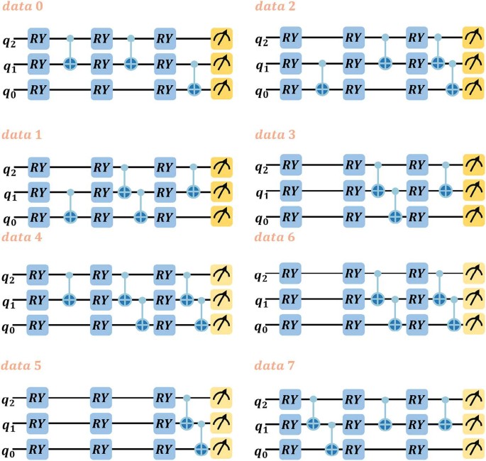
The designed quantum circuits of \(U_{2} ( \theta _{2} )\) for data 0–data 7

So far, we have identified a relatively optimal structure for \(U_{2} ( \theta _{2} )\). Similarly, one can find a relatively optimal structure for \(U_{1} ( \theta _{1} )\) in a similar manner, which will not be elaborated here. Notably, the \(U_{1} ( \theta _{1} )\) circuit used in the experiments of this paper is an unoptimized HEA ansatz. Using these two circuits, we complete the quantum state encoding process for classical data.
Subsequently, we initiate the similar calculation between target data T and the element in the database based on the Long’s algorithm, with the specific process as outlined below. The states that overlap with \(\mid T ' \rangle \) are first marked by the oracle operation with a phase rotation angle 0.677π, which is calculated according to Long’s algorithm, and then their amplitudes are amplified by the diffusion operator with the same phase rotation angle. These two phase rotation operations are realized by two Multi-controlled Phase gate (MCP) as shown in Fig. 1. Given the scale of the database is 8, the above process only requires one iteration. Note that the above steps are performed using Qiskit [47], which is an open-source quantum computing framework developed by IBM.
Finally, we measure all quantum bits and read the measurement results. We can categorize the results into successful outcomes and unsuccessful outcomes. Successful outcomes refer to measurements of the \(n_{D}\) bits yielding 0, while unsuccessful outcomes are those where this part is non-zero. We post-select these successful results, where the index i of the state with the highest probability, that is “000”, is denoted as \(i^{*}\). Considering the problem setup where the target data is defined as an all-black image, i.e., the 0-th image in the database, the target index should be “000”. These aligns with the results obtained by our algorithm as shown in the first subfigure of Fig. 7, indicating the successful completion of the pattern-matching task. To further elucidate the performance of the proposed algorithm, we made several different comparisons.
In evaluating the performance of different quantum pattern matching algorithms with different quantum circuits, that are searched or optimized structure, denoted as AQ, the un-optimized one, denoted as AA, and exact encoding circuit, denoted as EE, we conducted a comprehensive analysis based on several key metrics. The algorithms under consideration include a basic algorithm for computing similarity, denoted as N in the resulting pictures Fig. 5, Fig. 8, Fig. 9, and Fig. 11, which calculates the similarity between the target and the element in the database by only performing encoding operator (\(U_{1}\) and \(U_{2}^{\dagger}\)) without performing any probability amplitude amplification operations, schemes based on Grover’s search algorithm, denoted as G in the resulting pictures Fig. 6, Fig. 8, Fig. 9, Fig. 11, which executes two phase inversions in the process of marketing and amplitude amplification, and our scheme based on Long’s algorithm,denoted as L in the resulting pictures Fig. 7, Fig. 8, Fig. 9, Fig. 11. The evaluation criteria encompassed factors such as the success probability, the accuracy and the computational complexity.

The comparison of the results of image pattern matching using different numbers of CNOT gates without amplification. The title of each subfigure is the target data in its situation, the x-coordinate represents the eight results with higher probability obtained by measurement in two cases respectively, ‘rest’ is the probability of remaining outcome and the y-coordinate is the corresponding value. Finally, the bar with the color watermelon red represents the output of the case with more gates, and the bar with the color grayish-blue represents that with fewer gates. Notably, here and in the following only the structure of \(U_{2}\) is optimized

The comparison of results of image pattern matching using different numbers of CNOT gates based GSA. The bar with the color orange represents the output of the case with more gates, and the bar with the color sky blue represents that with fewer gates

The comparison of the results of image pattern matching using different numbers of CNOT gates based on Long’s algorithm. The red bar represents the output of the case with more gates and the blue one represents that with fewer gates. The outcome shows that the successful probability of completing pattern matching is considerably enhanced and the ‘failure’ (not exactly) probability, i.e., the value of bar ‘rest’ greatly depressed

The comparison of the results of image pattern matching with exact encoding based on three algorithms. The title of every subfigure is the target data in its situation, the x-coordinate is the eight results with higher probability obtained by measurement in three cases respectively, ‘rest’ is the probability of remaining outcome and the y-coordinate is the corresponding value

The comparison of the results of image pattern matching using fewer CNOT gates based on three algorithms. The title of every subfigure is the target data in its situation, the x-coordinate is the eight results with higher probability obtained by measurement in three cases respectively, ‘rest’ is the probability of remaining outcome and the y-coordinate is the corresponding value
In the context of the problem setup in this section, the measurement results of these three algorithms accomplishing the pattern matching task based on distinct circuits are depicted in Fig. 5 through Fig. 11.
First, we showcase the output accuracy (i.e., the probability of correctly completing the pattern-matching) achieved by three algorithms on three circuits as shown in Fig. 5 through Fig. 9, comparing them from five different perspectives illustrated in Fig. 10. Figure 5 is the comparison of the results of algorithm N on AA and AQ. The figure displays the measurement results obtained when each of the 8 images from the database is considered as the target data. The horizontal axis represents the measurement results of 6-qubit quantum bits, where the first three bits represent \(n_{D}\)-bits, and the latter three bits represent \(n_{X}\)-bits. The vertical axis represents the measurement probability corresponding to each measurement result. The bars in the graph depict the eight highest probability outcomes, while ‘rest’ represents the collection of all other outcomes. As no amplification has been applied, the average maximum probability of correct results should not exceed \(\frac{1}{8}\). Our experimental results align with the expected outcome. Further, the result demonstrates that the searched structure firstly can complete the task correctly and then, by contrast, can achieve comparative or even better performance with fewer quantum gates. To further assess the performance of the optimized structure AQ, we conduct algorithms G and L on it, and compared the results with those obtained on the structure before optimization, that is AA, as shown in Fig. 6 and Fig. 7. The meanings of the horizontal and vertical axes in these figures are the same as in Fig. 5. In both of these algorithms, AQ demonstrates comparable accuracy to the previous structure AA on average and performed well in completing the tasks. Through the comparison of these three experiments, we effectively highlight the efficacy of the searched optimized structure, that is, the output precision of AQ is comparable to or better than that of its more resource-intensive version AA, which indicates that our scheme could be used for some problems without strict precision requirements, such as the calculation of the global trend of the financial market indicator.

Partial experimental design framework. The horizontal axis represents abbreviations for the executed algorithms in the experiment, while the vertical axis denotes abbreviations for the circuits employed in the experiment. Each point in the graph represents an experiment conducted under the specified conditions at the corresponding coordinates
Figure 8 and Fig. 9 present the experimental results of three algorithms executed on the AA and AQ, respectively, with the same settings for the horizontal and vertical axes as in Fig. 5. In contrast to Fig. 5 and Fig. 7, which showcase circuit performance, the purpose is to provide a clearer horizontal comparison of the output accuracy of the three algorithms. By examining whether the amplitude amplification operation is performed, the results indicate that the accuracy of the two algorithms executing this operation is higher. For example, the probability of correctly matching data-0 in Algorithm G is approximately 1.6 times that of Algorithm N, clearly demonstrating the functionality of amplitude amplification operation. In terms of overall execution performance, Algorithm L, our proposed algorithm, exhibits significantly higher output accuracy compared to Algorithm G. The probability of correctly matching data-0 in Algorithm L is nearly 2.5 times that of Algorithm N and almost 1.5 times that of Algorithm G. The above results intuitively reflect, from a mathematical perspective, the improvement in our algorithm’s accuracy in successfully completing the task. In comparison, data-4’s circuit performance is relatively poor in our scheme, but it can still complete the task of pattern matching with a better than other two algorithms.
Considering the 5 result graphs mentioned earlier, our algorithm outperforms existing quantum pattern matching algorithms based on GSA that use exact encoding by achieving the pattern task with fewer computational resources and higher precision, which makes the scheme more appropriate for NISQ [48] device to emerge.
Secondly, we focus on the success probabilities denoted as ′Prob′ of the three algorithms in accomplishing quantum pattern matching tasks on AQ. It should be noted that ′Prob′ refers to the sum of the probabilities of results whose \(n_{D}\) bits are measuring as “000”, which indicates that the obtained states overlap with \(\vert 0 \rangle ^{\otimes 3}\), differing from the definition of ‘accuracy’ mentioned before. The sum of the remaining result probabilities represents the failure probability. For brevity, only the comparison for the case of T = data-0 is given in Fig. 11. The horizontal and vertical axes in Fig. 11 are set the same as in Fig. 5, systematically displaying all possible measurement outcomes. A comparison of the results between Algorithm N and Algorithm G shows a significant reduction in the failure probability for Algorithm G, attributed to the amplitude amplification operation. Algorithm L, building upon this, further reduces the failure probability or, in other words, suppresses the probability amplitude of states that do not overlap with the \(\vert 0 \rangle ^{\otimes 3}\) state. Concretely, the result shows that our scheme can achieve a successful probability of 95% while the other two schemes can only achieve the probabilities of 46.2% and 71%, respectively, which verifies the effectiveness of our proposal. A higher success probability implies fewer repetitions of algorithm execution needed to obtain measurement results, further reducing the computational resources consumed by the algorithm, such as quantum state. This makes our scheme more efficient and practically executable.

The comparison of the successful probability of image pattern matching using different number CNOT gates based on three algorithms. The title of every subfigure is the target data in its situation, the x-coordinate is all of the measurement outcomes without postselection in three cases respectively and the y-coordinate is the corresponding value. The successful probability of pattern matching is the sum of the probabilities of the results whose \(n_{D}\) bits are represented by the first three digits of abscissa being 0
Finally, we analyze the query complexity (number of executions of the oracle) and circuit size of the proposed algorithm. Long’s algorithm is a variant of GSA, with smaller phase rotation angles executed during queries. Therefore, the relationship between the query count \(k_{\mathrm{op}} '\) of Long’s algorithm and the query count \(k_{\mathrm{op}}\) of GSA is: \(k_{\mathrm{op}} ' \geq k_{\mathrm{op}} \). Such that the query complexity of our quantum pattern matching scheme remains the same to be \(O( \sqrt{N} )\). Next we discuss the size of the circuit for implementing our algorithm. In the context of the problem setting in this section, our algorithm requires preparing a database state of six qubits and a target data state of three qubits. If the former is prepared using traditional exact encoding circuits, it would require 32 six-qubit Toffoli gates, which can be decomposed into 128 CNOT gates. As for the latter, it would require one Toffoli gate, which need 6 CNOT gates [49]. If considering the case where some quantum computing devices only allow nearest-neighbor interactions between qubits, then the approximate number of CNOT gates required to prepare an arbitrary n-qubit quantum state on an initialized quantum circuit is:
showing an exponential relationship with the number of bits, n. If method in [30] is employed, the database state preparation would require 30 CNOT gates, and the target data state preparation would need 6 CNOT gates. The circuit depth, gate count, and the relationship with the number of bits are \(O(\mathrm{poly}(n))\) and \(O(n)\), respectively. In our approach, the number of gates needed to prepare these two states will be further reduced. Taking the target data state preparation as an example, the average number of required CNOT gate in our scheme is approximately 3 as shown in Fig. 4. As for the complexity, it still maintains to be \(O(\mathrm{poly}(n))\) in depth and \(O(n)\) in multi-qubit gate. Correspondingly, as a trade-off, when running the same algorithm, the output accuracy of our optimized structure may be slightly lower than that of precise encoding, but comparable to the accuracy achieved using method in [30], and enough to properly solve the problems that do not need exact encoding.
4 Conclusion
In this study, we propose a quantum pattern matching scheme based on QASA and Long’s algorithm, which significantly improves the performance through the optimization of circuit structures and a customized phase rotation angle. Specifically, we first optimized the gate layout of the encoding circuit based on QASA. In comparison to existing solutions, our approach uses fewer two-qubit entangling gates, exhibiting a linear relationship with the number of bits rather than an exponential one, making it a more computationally option. Building upon this foundation, we significantly enhanced the success probability of the quantum pattern matching algorithm using Long’s Algorithm. This implies a substantial reduction in the number of algorithm iterations required to obtain measurement results, further conserving computational resources. To validate the correctness and effectiveness of our approach, we took a simple instance of image pattern matching as an example and compared the performance of different algorithms on various circuit structures from both horizontal and vertical perspectives, as illustrated in Fig. 10. The results indicate that, compared to existing algorithms based on GSA and exact encoding, as well as existing schemes based on GSA and AAE, our approach can achieve the pattern matching task with higher accuracy while using fewer quantum computational resources. Hence, it will help with immediate and practical applications for NISQ devices.
Meanwhile, our algorithm demonstrated notable advancements in circuit size and success probability of the quantum pattern matching, offering valuable insights for future quantum computing research. Nevertheless, we acknowledge the limitations of this study, for example, our circuit optimization process is completed using gradient descent, and during this process, there is a possibility of encountering the phenomenon of gradient vanishing, commonly known as the ‘barren plateau’. For future research, we recommend further exploration of the application of quantum search algorithm in classical computing fields such as artificial intelligence. This field still holds many unresolved mysteries, and we look forward to more researchers joining in and making breakthroughs. This study contributes to the development of the quantum computing field, laying the foundation for broader research endeavors.
Data availability
Simulation data are available from the corresponding author upon reasonable request.
Abbreviations
- NISQ:
-
noisy intermediate-scale quantum devices
- GSA:
-
Grover search algorithm
- PQC:
-
parameterized quantum circuit
- QASA:
-
quantum circuit architecture search algorithm
- AAE:
-
approximate amplitude encoding
- VQA:
-
quantum learning algorithm
- MMD:
-
maximum mean discrepancy
- CNOT:
-
controlled-not gate
References
Navarro G. A guided tour to approximate string matching. ACM Comput Surv. 2001;33(1):31–88.
Crochemore M, Hancart C, Lecroq T. Algorithms on strings. Cambridge: Cambridge University Press; 2007.
Knuth DE, Morris JH Jr, Pratt VR. Fast pattern matching in strings. SIAM J Comput. 1977;6(2):323–50.
Boyer RS, Moore JS. A fast string searching algorithm. Commun ACM. 1977;20(10):762–72.
Lu B, Fan C-R, Liu L, Wen K, Wang C. Speed-up coherent Ising machine with a spiking neural network. Opt Express. 2023;31(3):3676–84.
Fan C-R, Lu B, Feng X-T, Liu L, Wang C. Efficient multi-qubit quantum data compression. Quantum Eng. 2021;3(2):e67
Lu B, Liu L, Song J-Y, Wen K, Wang C. Recent progress on coherent computation based on quantum squeezing. AAPPS Bull. 2023;33(1):7.
Song J, Lu B, Liu L, Wang C. Noisy quantum channel characterization using quantum neural networks. Electronics. 2023;12(11):2430.
Lu B, Gao Y-P, Wen K, Wang C. Combinatorial optimization solving by coherent Ising machines based on spiking neural networks. Quantum. 2023;7:1151.
Bartolucci S, Birchall P, Bombin H, Cable H, Dawson C, Gimeno-Segovia M, Johnston E, Kieling K, Nickerson N, Pant M et al.. Fusion-based quantum computation. Nat Commun. 2023;14(1):912.
Zhong H-S, Wang H, Deng Y-H, Chen M-C, Peng L-C, Luo Y-H, Qin J, Wu D, Ding X, Hu Y et al.. Quantum computational advantage using photons. Science. 2020;370(6523):1460–3.
Willsch D, Willsch M, De Raedt H, Michielsen K. Support vector machines on the d-wave quantum annealer. Comput Phys Commun. 2020;248:107006.
Deutsch D, Jozsa R. Rapid solution of problems by quantum computation. Proc R Soc Lond Ser A, Math Phys Sci. 1992;439(1907):553–8.
Shor PW. Algorithms for quantum computation: discrete logarithms and factoring. In: Proceedings 35th annual symposium on foundations of computer science. New York: IEEE; 1994. p. 124–34.
Grover LK. Quantum mechanics helps in searching for a needle in a haystack. Phys Rev Lett. 1997;79(2):325.
Biamonte J, Wittek P, Pancotti N, Rebentrost P, Wiebe N, Lloyd S. Quantum machine learning. Nature. 2017;549(7671):195–202.
Tacchino F, Macchiavello C, Gerace D, Bajoni D. An artificial neuron implemented on an actual quantum processor. npj Quantum Inf. 2019;5(1):26.
Cong I, Choi S, Lukin MD. Quantum convolutional neural networks. Nat Phys. 2019;15(12):1273–8.
Beer K, Bondarenko D, Farrelly T, Osborne TJ, Salzmann R, Scheiermann D, Wolf R. Training deep quantum neural networks. Nat Commun. 2020;11(1):808.
Wei S, Chen Y, Zhou Z, Long G. A quantum convolutional neural network on nisq devices. AAPPS Bull. 2022;32:1–11.
Hur T, Kim L, Park DK. Quantum convolutional neural network for classical data classification. Quantum Mac Intell. 2022;4(1):3.
Ramesh H, Vinay V. String matching in o \((n+m)\) quantum time. J Discret Algorithms. 2003;1(1):103–10.
Montanaro A. Quantum pattern matching fast on average. Algorithmica. 2017;77:16–39.
Soni KK, Rasool A. Pattern matching: a quantum oriented approach. Proc Comput Sci. 2020;167:1991–2002.
Soni KK, Rasool A. Quantum-based exact pattern matching algorithms for biological sequences. ETRI J. 2021;43(3):483–510.
Menon V, Chattopadhyay A. Quantum pattern matching oracle construction. Pramana. 2021;95(1):22.
Jiang H, et al. A pattern matching-based framework for quantum circuit rewriting. 2022. arXiv preprint. arXiv:2206.06684.
Giovannetti V, Lloyd S, Maccone L. Quantum random access memory. Phys Rev Lett. 2008;100(16):160501.
Tezuka H, Nakaji K, Satoh T, Yamamoto N. Grover search revisited: application to image pattern matching. Phys Rev A. 2022;105(3):032440.
Nakaji K, Uno S, Suzuki Y, Raymond R, Onodera T, Tanaka T, Tezuka H, Mitsuda N, Yamamoto N. Approximate amplitude encoding in shallow parameterized quantum circuits and its application to financial market indicators. Phys Rev Res. 2022;4(2):023136.
Du Y, Huang T, You S, Hsieh M-H, Tao D. Quantum circuit architecture search for variational quantum algorithms. npj Quantum Inf. 2022;8(1):62.
Long G-L. Grover algorithm with zero theoretical failure rate. Phys Rev A. 2001;64(2):022307.
Long GL, Li YS, Zhang WL, Niu L. Phase matching in quantum searching. Phys Lett A. 1999;262(1):27–34.
Benedetti M, Lloyd E, Sack S, Fiorentini M. Parameterized quantum circuits as machine learning models. Quantum Sci Technol. 2019;4(4):043001.
Kandala A, Mezzacapo A, Temme K, Takita M, Brink M, Chow JM, Gambetta JM. Hardware-effcient variational quantum eigensolver for small molecules and quantum magnets. Nature. 2017;549(7671):242–6.
Cerezo M, Arrasmith A, Babbush R, Benjamin SC, Endo S, Fujii K, McClean JR, Mitarai K, Yuan X, Cincio L et al.. Variational quantum algorithms. Nat Rev Phys. 2021;3(9):625–44.
Bharti K, Cervera-Lierta A, Kyaw TH, Haug T, AlperinLea S, Anand A, Degroote M, Heimonen H, Kottmann JS, Menke T et al.. Noisy intermediate-scale quantum algorithms. Rev Mod Phys. 2022;94(1):015004.
Elsken T, Metzen JH, Hutter F. Neural architecture search: a survey. J Mach Learn Res. 2019;20(1):1997–2017.
Bittel L, Kliesch M. Training variational quantum algorithms is np-hard. Phys Rev Lett. 2021;127(12):120502.
Liu J-G, Wang L. Differentiable learning of quantum circuit born machines. Phys Rev A. 2018;98(6):062324.
Coyle B, Mills D, Danos V, Kashefi E. The born supremacy: quantum advantage and training of an Ising born machine. npj Quantum Inf. 2020;6(1):60.
Sriperumbudur BK, Gretton A, Fukumizu K, Lanckriet G, Schölkopf B. Injective Hilbert space embeddings of probability measures. In: 21st annual conference on learning theory (COLT 2008). Omnipress; 2008. p. 111–22.
Gretton A, Fukumizu K, Teo C, Song L, Schölkopf B, Smola A. A kernel statistical test of independence. Advances in neural information processing systems. 2007;20.
Bergholm V, et al. PennyLane: automatic differentiation of hybrid quantum-classical computations. 2018. arXiv:1811.04968.
Nielsen MA, Chuang I. Quantum computation and quantum information. 2002.
Crooks GE. Gradients of parameterized quantum gates using the parameter-shift rule and gate decomposition. 2019. arXiv preprint. arXiv:1905.13311.
Anis MS, Abraham H, Offei A, Agarwal R, Agliardi G, Aharoni M, Akhalwaya IY, Aleksandrowicz G, Alexander T, Amy M, Anagolum S, Arbel E, Asfaw A, Athalye A, Avkhadiev A, Azaustre C, Bhole P, Banerjee A, Banerjee S, Bang W, Bansal A, Barkoutsos P, Barnawal A, Barron G, Barron GS, Bello L, et al. Qiskit: an open-source framework for quantum computing. 2021. https://doi.org/10.5281/zenodo.2573505.
Preskill J. Quantum computing in the nisq era and beyond. Quantum. 2018;2:79.
Maslov D. Advantages of using relative-phase Toffoli gates with an application to multiple control Toffoli optimization. Phys Rev A. 2016;93(2):022311.
Funding
The authors gratefully acknowledge the support from the National Natural Science Foundation of China through Grants Nos. 62131002, 62371050 and 62071448, and the Fundamental Research Funds for the Central Universities (BNU).
Author information
Authors and Affiliations
Contributions
L. L. and C. W. designed the scheme. L. L. performed the derivation of the theoretical work. L. L. and X. W. carried out the simulation works. C. W. supervised the study. All authors participated in discussions of the results. All authors have accepted responsibility for the entire content of this manuscript and approved its submission.
Corresponding author
Ethics declarations
Ethics approval and consent to participate
Not applicable.
Competing interests
The authors declare no competing interests.
Additional information
Publisher’s Note
Springer Nature remains neutral with regard to jurisdictional claims in published maps and institutional affiliations.
Rights and permissions
Open Access This article is licensed under a Creative Commons Attribution 4.0 International License, which permits use, sharing, adaptation, distribution and reproduction in any medium or format, as long as you give appropriate credit to the original author(s) and the source, provide a link to the Creative Commons licence, and indicate if changes were made. The images or other third party material in this article are included in the article’s Creative Commons licence, unless indicated otherwise in a credit line to the material. If material is not included in the article’s Creative Commons licence and your intended use is not permitted by statutory regulation or exceeds the permitted use, you will need to obtain permission directly from the copyright holder. To view a copy of this licence, visit http://creativecommons.org/licenses/by/4.0/.
About this article

Cite this article
Liu, L., Wu, XY., Xu, CY. et al. The deterministic pattern matching based on the parameterized quantum circuit. EPJ Quantum Technol. 11, 3 (2024). https://doi.org/10.1140/epjqt/s40507-023-00215-9
Received:
Accepted:
Published:
DOI: https://doi.org/10.1140/epjqt/s40507-023-00215-9