Infrared finiteness of a complete theory of charged scalars and fermions at finite temperature

Abstract

It is known that the infrared (IR) divergences accruing from pure fermion–photon interactions at finite temperature cancel to all orders in perturbation theory. The corresponding infrared finiteness of scalar thermal QED has also been established recently. Here, we study the IR behaviour, at finite temperature, of theories where charged scalars and fermions interact with neutrals that could potentially be dark matter candidates. Such thermal field theories contain both linear and sub-leading logarithmic divergences. We prove that the theory is IR-finite to all orders in perturbation, with the divergences cancelling order by order between virtual and real photon corrections, when both absorption and emission of photons from and into the heat bath are taken into account. The calculation follows closely the technique used by Grammer and Yennie for zero temperature field theory. The result is generic and applicable to a variety of models, independent of the specific form of the neutral-fermion–scalar interaction vertex.

1 Introduction

We are interested here in addressing the infrared (IR) behaviour of theories with both charged scalars and fermions, interacting with neutral singlets or doublets, at finite temperature. The study is motivated by simple models of dark matter (DM), described by a Lagrangian density of the type [1],

(1)

This is an extension of the Standard Model (SM), containing a charged lepton f, with an additional charged scalar $\phi ^+$, along with the $SU(2) \times U(1)$ singlet neutral Majorana fermion $\chi$ which is usually the dark matter candidate. Note that we have written only the part of the lagrangian that is relevant to our analysis, suppressing the rest. For example, if f is part of the usual left-handed doublet, then so must $\phi ^+$ be. Similarly, we could have f to be a quark field, with $\phi$ now being a charged colored scalar. However, this would necessitate the discussion of QCD interactions, which, while being analogous to the electromagnetic interactions, is associated with additional computational complexity that is not germane to the issue at hand.

It might seem that the Lagrangian of Eq. 1 is too specific and too simplistic a choice. However, not only is it a perfectly viable stand-alone model by itself (modulo the rest of the SM fields), but it also captures the essence of a wide class of models. For example, consider the rather popular case of the minimal supersymmetric standard model (MSSM), which can be realised by identifying $\chi$ with a bino and the $\phi ^+$ with the supersymmetric partner of a SM fermion, say the positron.¹ And, whereas the MSSM spectrum would include, apart from the SM particles, the entire gamut of their supersymmetric partners, only a handful of them play a significant role in determining the relic density.

Although, generically, the DM itself is a linear combination of the bino, the neutral wino and the two neutral higgsinos, for a very large class of supersymmetry breaking scenarios, the higgsino mass parameter $\mu$ is much larger than the soft terms ($M_{1,2}$) for the gauginos, thereby suppressing the higgsino component to negligible levels. And since the wino-bino mixing is pivoted by $\mu$, a large value for the latter also suppresses the wino-component in the DM. The assumption of a bino-like DM further simplifies the calculations as we may safely neglect additional diagrams, e.g., with s-channel gauge bosons or Higgs.² It should also be appreciated that no new infrared divergence structures would appear even on the inclusion of such additional mediators.³ In other words, restricting ourselves to the particular case of the bino does not represent the neglect of subtle issues while allowing for considerable simplifications, both algebraic and in book-keeping. In this paper, we shall interchangeably use the words bino and DM.

It has been shown in Ref. [1] that the thermal field theory corresponding to Eq. 1 is IR-finite up to next-to-leading order (NLO) in soft-photon corrections; in addition, the finite remainder has been computed to NLO in this paper as well, and the importance of this thermal correction in calculations of dark matter relic densities in the early Universe has also been highlighted.

In the present paper, we study this same Lagrangian density for specificity, with the motivation to extend the NLO result of Ref. [1] to all orders in perturbation theory and hence obtain the all-order proof of IR finiteness of such theories. While obtaining this proof, we incidentally confirm the IR-finiteness result of Ref. [1] to NLO, although, unlike them, we do not explicitly compute the IR-finite piece. We also show in the end that the result is independent of the actual form of the neutral-fermion-scalar vertex, and hence applies to a class of such models.

We assume here that the DM particle freezes out after the electro-weak transition; hence, only electromagnetic interactions are relevant for the IR finiteness at these scales.⁴

We begin by addressing the higher-order corrections to processes such as,

$$\begin{aligned} \chi + \overline{\chi } \leftrightarrow f + \overline{f}, \quad \text {and} \quad \chi + f \rightarrow \chi + f , \end{aligned}$$

(2)

where the interaction is mediated by vertices of the type $\chi$–$\phi$–f, which are relevant for DM annihilation or scattering off a SM particle. This is illustrated in Fig. 1. Higher order electromagnetic corrections to such diagrams involve virtual photon exchanges as well as real photon emissions from either f or $\phi$.

Fig. 1

A typical dark matter annihilation/scattering process

Such contributions can be calculated in a real time formulation of the thermal field theory [2,3,4]. In Ref. [5], the eikonal approximation was used and the interaction of photons with a semi-classical current was analysed within the framework of thermal field theory. In Ref. [6], 1-loop corrections to thermal QED were computed for both fermions and scalars. It was found that the finite temperature mass shift for scalar QED when the temperature is less than the scalar mass ($0 < T \ll m_s$) is identical to the corresponding fermion case as is the IR divergent piece of the wave function and vertex renormalisation constants. However, the contribution to the plasma screening mass was twice that for the fermion loop due to the difference in the form of the thermal distributions (boson versus fermion).

The approach of Grammer and Yennie [7] (henceforth referred to as GY) which was used to prove the IR finiteness to all orders of fermionic QED at zero temperature was extended to prove the IR finiteness of a thermal field theory of purely fermionic QED [8]. The same approach was used to prove the IR finiteness of a thermal theory of pure charged scalars, that is, thermal scalar QED [9]. In this approach, the photon propagator (for virtual photon insertions) and the polarisation sum (for real photon insertions) can be expressed as a sum over the so-called K and G photons ($\widetilde{K}$ and $\widetilde{G}$ photons for the case of real photons). GY showed that the IR divergences are contained in the K and $\widetilde{K}$ photon contributions while the G and $\widetilde{G}$ photon contributions are IR finite, and that the IR divergences cancel order-by-order between the virtual (K) photon and real ($\widetilde{K}$) photon contributions respectively.

Here we use a similar approach to address the issue of IR finiteness of the thermal field theory corresponding to Eq. 1, thereby combining and extending the results of the earlier work on thermal fermions and thermal charged scalars.

The paper is organised as follows. In Sect. 2, we set up the real-time formulation of the thermal field theory corresponding to the Lagrangian of Eq. 1 and write down the propagators and vertex factors of the theory. Since the calculation heavily depends on understanding the approach of Grammer and Yennie, in Sect. 3 we begin by defining the so-called K and G photon insertions for virtual and real photons. For completeness and clarity, we also list the main results obtained in the earlier calculations of thermal fermionic [8] and scalar QED [9] respectively and also highlight how the IR divergences are contained in the K photon contribution while the G photon contributions are IR finite. In Refs. [5, 8, 10] it was shown that pure fermionic thermal QED has both a linear divergence and a logarithmic subdivergence in the infrared compared to the purely logarithmic divergence encountered in the zero temperature theory, owing to the nature of the thermal photon propagator. The same was true for the case of thermal scalar QED as shown in Ref. [9] and will be found to be true in the current case as well. The divergences factorise and exponentiate and cancel order by order between virtual and real photon contributions (the latter include both emission and absorption terms); this same approach will be used to prove the IR finiteness to all orders in perturbation of the thermal theory corresponding to the Lagrangian, Eq. 1.

After this overview, we then set up the relevant machinery in Sect. 4 to address the present problem of infrared (IR) finiteness of the complete theory of the particles $\chi$ interacting with charged fermions f and scalars $\phi$; in particular, we apply the technique of GY to the process⁵$\chi f \rightarrow \chi f$. We would establish that the G photon insertions give rise to contributions exactly analogous to those arising in pure fermionic and scalar thermal QED [8, 9] and, hence, earlier results can, essentially, be taken over in toto. Similarly, the real photon (both $\widetilde{K}$ and $\widetilde{G}$) contributions arise from a straightforward application of earlier results [8, 9] as well, as also discussed in Sect. 3. Hence it is the virtual K photon insertions that lead to the main new results of this paper, and is dealt with in detail in Sect. 4.

Section 5 contains the discussions and conclusions, while Appendix A is used to list some useful identities for thermal field theories that are used to factorise the K photon contributions.

Before we proceed, a few remarks are in order. The $\chi$ interacts only with fermions and the scalar (sfermion) $\phi$, and not with the photon. Thus, only the charged scalar interactions with $\chi$ are shown in Eq. 1 since it is the resummation of the radiative photon diagrams which are of interest here. Finally, we will see that the results we obtain do not depend on the exact form of the $\chi$–f–$\phi$ vertex and is hence applicable to a larger class of such theories.

2 Real-time formulation of thermal field theory

For the sake of completeness, we begin by briefly reviewing the real-time formulation [2,3,4] of thermal (scalar, fermion and photon) fields in equilibrium with a heat bath at temperature T. This is a statistical field theory with a thermal vacuum defined such that the ensemble average of an operator can be written [4] as the expectation value of time-ordered products in the thermal vacuum. In order to satisfy this requirement, a special path needs to be chosen for the integration in the complex time plane.

In the corresponding path integral formulation, the generating functional $Z_C(\beta ; j)$ (where $Z_C(\beta ;0)$ is the usual partition function) is used to define averages/expectation values of time ordered products where the time ordered path C is in a complex time plane from an initial time, $t_i$ to a final time, $t_i - i \beta$, where $\beta$ is the inverse temperature of the heat bath, $\beta = 1/T$; see Fig. 2. The consequence is that these thermal fields satisfy the periodic boundary conditions,

$$\begin{aligned} \varphi (t_0) = \pm \varphi (t_0 - i \beta ), \end{aligned}$$

where $\pm 1$ correspond to boson and fermion fields respectively.

Fig. 2

Standard time path for real time formulation of thermal field theories. The type-1 and type-2 thermal fields “live” on the $C_1$ and $C_2$ paths of the contour

Of particular relevance are the pieces of the time path, $C_1$ and $C_2$, along the real time axis and parallel to it, respectively. This results in the well-known field doubling with fields that “live” on the $C_1$ or $C_2$ line; these are, thus, of either type-1 (physical) or type-2 (ghosts), with propagators acquiring a $2 \times 2$ matrix form. Only type-1 fields can occur on external legs while fields of both types can occur on internal legs, with the off-diagonal elements of the propagator allowing for conversion of one type into another. The zero temperature part of the propagator corresponds to the exchange of a virtual particle, as usual, and the finite temperature part of the propagator represents an on-shell contribution.

Hence, the Lagrangian corresponding to a thermal field theory of neutrals interacting with charged scalars and fermions can be written down, starting from the zero-temperature Lagrangian given in Eq. 1 [11,12,13,14]. This gives both the propagators as well as vertex factors relevant to the thermal theory.

2.1 The propagators

The thermal scalar propagator at zero chemical potential is given by

$$\begin{aligned}&i {{S}}_\mathrm{scalar}^{t_a, t_b} (p,m)=\left( \begin{array}{cc} \Delta (p) &{} 0 \\ 0 &{} \Delta ^*(p) \end{array} \right) \nonumber \\&\quad +\, 2 \pi \delta (p^2-m^2) N_\mathrm{B}(\vert p^0 \vert ) \left( \begin{array}{cc} 1 &{} e^{\vert p^0 \vert /(2T)} \\ e^{\vert p^0 \vert /(2T)} &{} 1 \end{array} \right) , \end{aligned}$$

(3)

where $\Delta (p) = i/(p^2-m^2+i\epsilon )$, and $t_a, t_b (=1,2)$ refer to the field’s thermal type. The first term in each case corresponds to the $T=0$ part and the second to the finite temperature piece; note that the latter contributes only on mass-shell. We shall shortly discuss the bosonic number density $N_\mathrm{B}(\vert p^0 \vert )$.

Similarly, in the Feynman gauge, the photon propagator corresponding to a momentum k can be expressed as

$$\begin{aligned} i {D}^{t_a,t_b}_{\mu \nu } (k) = -g_{\mu \nu } i {D}^{t_a,t_b} (k) = - g_{\mu \nu } \, i {{S}}_\mathrm{scalar}^{t_a, t_b} (k,0). \end{aligned}$$

(4)

On the other hand, the thermal fermion propagator at zero chemical potential is given by

(5)

where , and ; hence the fermion propagator is proportional to .

While the fermionic number operator, viz.,

$$\begin{aligned} N_\mathrm{F}(\vert {p^0} \vert ) \equiv \frac{1}{\exp \{\vert p^0 \vert /T\} + 1} \; {\mathop {\longrightarrow }\limits ^{p^0 \rightarrow \,0}} \; \frac{1}{2}, \end{aligned}$$

(6)

is well-defined in the soft limit, the bosonic number operator in the photon propagator contributes an additional power of ${k^0}$ in the denominator in the soft limit, since

$$\begin{aligned} N_\mathrm{B}(\vert k^0 \vert ) \equiv \frac{1}{\exp \{\vert k^0 \vert /T\} - 1} \; {\mathop {\longrightarrow }\limits ^{k^0 \rightarrow \,0}} \; \frac{T}{\vert k^0 \vert }. \end{aligned}$$

(7)

Hence, it can be seen that the leading IR divergence in the finite temperature part is linear rather than logarithmic as was the case at zero temperature. Consequently, there is a residual logarithmic subdivergence that must also be shown to cancel at finite temperatures, thus making the generalisation to the thermal case non-trivial.

2.2 The vertex factors

The fermion–photon vertex factor is $(-ie\gamma _\mu )(-1)^{t_\mu +1}$ where $t_\mu =1,2$ for the type-1 and type-2 vertices. The corresponding scalar–photon 3-vertex factor is $[-ie(p_\mu + p'_\mu )](-1)^{t_\mu +1}$ where $p_\mu$ ($p'_\mu$) is the 4-momentum of the scalar entering (leaving) the vertex. In addition, there is a 2-scalar–2-photon seagull vertex (see Fig. 3) with a factor of $[+2ie^2 g_{\mu \nu }](-1)^{t_\mu +1}$. All fields at a vertex are of the same type, with an overall sign between physical (type 1) and ghost (type 2) vertices.

Fig. 3

Allowed vertices for fermion–photon and scalar–photon interactions

The bino-scalar–fermion vertex factor at a vertex V is denoted as $\Gamma _V$; for details on Feynman rules for Majorana particles at zero temperature, see Ref. [15]. These rules apply to the type-1 thermal bino vertex; an overall negative sign applies as usual to the type-2 bino vertex; again all fields at a vertex are of the same type.

3 Overview of the GY technique and its application to thermal field theories

In Ref. [9], it was established that a field theory of charged scalars is IR finite to all orders both at $T=0$ and at finite temperature. The corresponding all-order proof for fermionic QED is already known [8]. We now apply and extend these two results to prove the IR finiteness to all orders of theories of dark matter at finite temperature. The proof involves obtaining a neat factorisation and exponentiation of the soft terms to all orders in the theory, with order by order cancellation between the IR divergent contributions of virtual and real photon corrections to the leading order contribution. In order to achieve this, we use the Grammer and Yennie approach [7]. In this section, we provide, for the sake of completeness, an overview of the technique, for both the fermionic and scalar cases, while the new results of this paper can be found in Sect. 4.

3.1 The Grammer and Yennie approach at $T=0$

We begin by briefly outlining the classic proof of GY [7] of the IR finiteness of zero temperature fermionic QED. This involves starting with an nth order contribution⁶ to the process $e(p) \gamma ^*(q) \rightarrow e(p')$ (where q is the hard momentum of the photon flowing in at the vertex V, and the remaining n photon momenta can be arbitrarily soft), and examining the effect of adding an additional virtual or real $(n+1)$th photon with momentum k to this graph in all possible ways. All insertions on the graph to the right⁷of the vertex V are classified as insertions on the (final) $p'$ leg; see Fig. 4, whereas those to the left of the vertex V are deemed to be insertions on the (initial) p leg. Hence there are three possibilities for virtual photon insertions, viz., both vertices of the $(n+1)$th virtual photon being inserted on the $p'$ leg, both inserted on the p leg, and finally, one vertex inserted on each leg.

Fig. 4

Typical nth order diagram for $\gamma ^* f \rightarrow f$ discussed by GY, with r (s) photon insertions on the p ($p'$) leg, with $r+s=m$

To separate out the IR divergent piece in a virtual photon insertion, the corresponding photon propagator of the newly inserted photon was written as a sum over so-called K- and G-photon contributions, viz.,

$$\begin{aligned}&-i \frac{g^{\mu {\nu }}}{k^2+i\epsilon } \nonumber \\&\quad = \frac{-i}{k^2+i\epsilon } \, \left\{ \left[ g^{\mu \nu } - b_k (p_f, p_i)\,k^\mu k^\nu \right] + \left[ b_k (p_f, p_i) k^\mu k^\nu \right] \right\} , \nonumber \\&\quad \equiv \frac{-i}{k^2+i\epsilon } \, \left\{ \left[ G\right] + \left[ K\right] \right\} . \end{aligned}$$

(8)

Here $b_k$ is a function of k as well as the momenta, $p_f$, $p_i$, where $p_f$ ($p_i$) corresponds to the momentum $p'$ or p depending on whether the final (initial) vertex of the $(n+1)$th photon was inserted on the $p'$ or p leg. To isolate all the IR divergences in the K-photon contributions, $b_k$ is defined to be

$$\begin{aligned}&b_k(p_f,p_i) \nonumber \\&\quad = \frac{1}{2} \left[ \frac{(2p_f-k) \cdot (2p_i-k)}{((p_f-k)^2-m^2)((p_i-k)^2-m'^2)} + (k \leftrightarrow -k) \right] , \nonumber \\&\quad = \frac{1}{2} \left[ \frac{(2p_f-k) \cdot (2p_i-k)}{(-2 p_f\cdot k + k^2)(-2p_i\cdot k +k^2)} + (k \leftrightarrow -k) \right] . \end{aligned}$$

(9)

Since the external particles are always on-shell, $p_f^2 = m^2$, $p_i^2 = m'^2$, and hence the $b_k$ are independent of the masses of the particles. Note that our definition of $b_k$ differs slightly from that of GY [7]; this modification is required to obtain the proper factorisation of the K photon terms and, more importantly, to show the IR finiteness of the G photon terms in the thermal case. Since the propagator is a sum over the K and G photon contributions, at every order, both the K and the G virtual photon are to be inserted, separately, to obtain the entire higher order graph.

Given the structure of the K-propagator, Eq. 8, a K photon insertion at a vertex $\mu$ is equivalent to the insertion $\gamma ^\mu k_\mu \equiv /{k}$ and the ensuing contribution can be expressed, courtesy generalised Feynman identities (see Eq. A.2, Appendix A), as the difference of two terms. Inserting the $(n+1)$th K photon vertex $\mu$ in all possible ways on the lower order graph thus gives sums of such contributions, leading to pair-wise cancellation between different contributions. Ultimately the contribution of the insertion of the $(n+1)$th virtual K photon is a single term, proportional to the lower order matrix element, $\mathcal{{M}}_n$. We show this later in greater detail for the thermal case in order to apply the results to our Lagrangian of interest, Eq. 1.

A similar separation of the polarisation sums for the insertion of real photons into so-called $\widetilde{K}$ and $\widetilde{G}$ contributions can be made. Here, the identification of the $\widetilde{K}$ and $\widetilde{G}$ photons occurs in the square of the matrix element, via,

$$\begin{aligned}&{\displaystyle }\sum \limits _\mathrm{pol} \epsilon ^*_\mu (k)\,\epsilon _\nu (k) \nonumber \\&\quad = {\displaystyle }- g_{\mu \nu }, \nonumber \\&\quad = {\displaystyle }-\left\{ \left[ g_{\mu \nu } - \tilde{b}_k(p_f,p_i) k_\mu k_\nu \right] + \left[ \tilde{b}_k(p_f,p_i) k_\mu k_\nu \right] \right\} , \nonumber \\&\quad \equiv {\displaystyle }-\left\{ \left[ \widetilde{G}_{\mu \nu }\right] + \left[ \widetilde{K}_{\mu \nu }\right] \right\} , \end{aligned}$$

(10)

where the tildes have been used to distinguish the real from the virtual photon contributions. Since $k^2=0$ for real photons, we define

$$\begin{aligned} \tilde{b}_k(p_f, p_i) = b_k(p_f, p_i)\Big |_{k^2 = 0} = \frac{p_f \cdot p_i}{ k\cdot p_f\; k\cdot p_i}, \end{aligned}$$

(11)

where $p_i$ ($p_f$) is the momentum $p'$ or p depending on whether the real photon insertion was on the $p'$ or p leg in the matrix element $\mathcal{M}_{n+1}$ (or its conjugate $\mathcal{M}_{n+1}^\dagger$). Again, GY showed that the insertion of a $\widetilde{K}$ real photon into an nth order graph leads to a cross section that is proportional to the lower order one. Details of this cancellation follow from the demonstration of the pair-wise cancellations that we show in the text below.

For both virtual and real photon insertions, the G ($\widetilde{G}$) photon contributions are IR finite with the entire IR divergent contribution being contained in the K (and $\widetilde{K}$) contributions. Combining the virtual and real photon contributions at every order, GY showed that the IR singularities cancel between the real and virtual contributions and hence the cross section for $e(p) \gamma ^*(q) \rightarrow e(p')$ is IR finite to all orders. We now specifically demonstrate the pair-wise cancellation for the virtual K photon insertion for the thermal case.

3.2 The GY approach in the thermal case

It was shown in Ref. [8] that a factorisation of the photon propagator into K and G types is possible in thermal fermionic QED as well because of the presence of the factor $g_{\mu \nu }$ in all components of the thermal photon propagator due to the vector nature of the photon, as seen from Eq. 4, so that Eq. 8 generalises in the thermal case to

$$\begin{aligned}&-i {g^{\mu {\nu }}} D^{t_a,t_b}(k) \nonumber \\&\quad = -i D^{t_a,t_b}(k) \left\{ \left[ g^{\mu \nu } - b_k (p_f, p_i)\,k^\mu k^\nu \right] + \left[ b_k (p_f, p_i) k^\mu k^\nu \right] \right\} , \nonumber \\&\quad \equiv -i D^{t_a,t_b}(k) \left\{ \left[ G\right] + \left[ K\right] \right\} . \end{aligned}$$

(12)

Furthermore, it was shown in Ref. [9] that similar results hold for the case of pure scalar thermal QED as well. Similarly, the polarisation sum for real thermal photons can also be expressed in terms of the $\widetilde{K}$ and $\widetilde{G}$ contributions. Hence it is possible to define $b_k(p_f, p_i)$ and $\tilde{b}_k (p_f, p_i)$ so that the IR divergences can be entirely subsumed into the K ($\widetilde{K}$) photon contribution, leaving the G ($\widetilde{G}$) contributions finite. We now outline the proof of this since this is relevant for the proof of IR finiteness of the Lagrangian corresponding to Eq. 1.

In both cases, the underlying process considered was the $2 \rightarrow 1$ process $\varphi (p) \gamma ^*(q) \rightarrow \varphi (p')$, $p+q = p'$, where $\varphi$ is appropriately a charged fermion or a charged scalar. Note that virtual corrections do not alter the energy-momentum conservation relation, but real photon corrections do; we discuss the implications of this later and assume for now that this equation holds in what follows. We start with the virtual photon insertions.

3.2.1 The GY approach in the thermal case: virtual K photon insertion

The matrix element corresponding to the process $\varphi (p) \gamma ^*(q) \rightarrow \varphi (p')$, $p+q = p'$, where $\varphi$ is a charged fermion, is given by

$$\begin{aligned} i \mathcal{M}_{0}^\mathrm{fermion}&= \left[ \bar{u}_{p'} \, \Gamma _V \, {u}_{p} \right] , \end{aligned}$$

(13)

where $\Gamma _V=-ie\gamma _V$ in the fermionic case. Consider the nth order correction to this lowest order contribution as shown in Fig. 4. The nth order graph with n added virtual photons has s vertices on the $p'$ leg and r vertices on the p leg, so that $r+s=m=2n$. We can express the nth order matrix element generically as

$$\begin{aligned}&i \mathcal{M}_{n}^\mathrm{fermion}\nonumber \\&\quad = (-ie)^{2n} (-1)^{\sum _{i=1}^{m} (t_i+1)} (i^m) \nonumber \\&\qquad \times \left[ \bar{u}_{p'} \gamma _{\mu _1} S^{t_1,t_2}_{p'+\sum _{1}} \, \gamma _{\mu _2} S^{t_2,t_3}_{p'+\sum _{2}} \, \cdots \, \gamma _{\mu _{s-1}} S^{t_{s-1},t_s}_{p'+\sum _{s-1}} \, \gamma _{\mu _{s}} S^{t_{s},t_V}_{p'+\sum _{s}} \right] \nonumber \\&\qquad \times \, \Gamma _V \times \left[ S^{t_V,t_r}_{p+\sum _{r}} \, \gamma _{\nu _r} S^{t_r,t_{r-1}}_{p+\sum _{r-1}} \, \gamma _{\nu _{r-1}} \cdots \, S^{t_2,t_1}_{p+\sum _{1}} \, \gamma _{\nu _1} {u}_{p} \right] \nonumber \\&\qquad \times \mathcal{D}^{\mu _1, \cdots , \mu _s; \nu _r, \cdots , \nu _1}_{[t_i]}, \nonumber \\&\quad = (-ie)^{2n} (-1)^{\sum _{i=1}^{m} (t_i+1)} (i^m) \times \left[ \mathcal{C}_{s}^{p'}\right] \times \Gamma _V \times \left[ \mathcal{C}_{r}^{p}\right] \times \mathcal{D}_n. \end{aligned}$$

(14)

Every vertex q occurs with a factor of $(-ie \times (-1)^{(t_q+1)})$, a factor of i is associated with each propagator, and $\Gamma _V$ is the vertex factor associated with the special vertex V where the momentum q enters. We see that $\Gamma _V$ separates the contributions from the $p'$ and p legs, shown in the square brackets in Eq. 14, and defined as the quantities $\mathcal{C}$. The subscripts on the $\mathcal{C}$s simply denote the number of vertices with photon insertions on the associated subdiagram as shown in Fig. 4. The notation is explained as follows. Photons enter the p leg with momenta $l_j$ at vertices j, with $j=1, \ldots , r$, while photons leave the $p'$ leg with momenta $l'_q$ at vertices q, with $q = 1, \ldots , s$; see Fig. 4. Note that this assumption of photon momentum direction is merely a convenient form of book-keeping and there is no loss of generality in this assumption. We have assumed that all photon insertions correspond to virtual photons and hence $r+s=m=2n$. The momentum to the right of the jth vertex on the p leg is thus $(p + \Sigma _{i=1}^j \, l_i) \equiv (p+\Sigma _j)$, while the momentum to the left of the qth vertex on the $p'$ leg is $(p' + \Sigma _{i=1}^{q} \, l'_i) \equiv (p'+\Sigma _q)$. Hence $S^{t_{q-1},t_q}_{p'+\sum _{q-1}}$ (with subscript ‘fermion’ suppressed for convenience) stands for the fermionic propagator from vertex ${q-1}$ to vertex q, corresponding to a momentum $p' + \sum _{i=1}^{q-1} l'_i$, while $S^{t_{j},t_{j-1}}_{p+\sum _{j-1}}$ stands for the corresponding propagator on the p leg from vertex j to ${j-1}$ with momentum $p + \sum _{i=1}^{j-1} l_i$. The superscripts on the fermion propagators $t_i$ refer to the thermal indices. Since all fields at a vertex have the same thermal type, the vertex q is associated with the thermal type $t_q$, etc.

Assuming for now that all photon insertions correspond to virtual photons,⁸ the contribution from the photon propagators, $\mathcal{D}_n$, is given by a product over n terms,

$$\begin{aligned} \mathcal{D}_n \equiv \mathcal{D}^{\mu _1, \ldots , \mu _s; \nu _r, \ldots , \nu _1}_{\{t_i\}} = \prod _{\{\alpha \beta \}} \int \frac{\mathrm{d}^4k_\alpha }{(2\pi )^4} \, \left[ -ig^{\alpha \beta } D^{t_\alpha ,t_\beta } \right] , \end{aligned}$$

(15)

where $\alpha ,\beta$ are any two of the dummy indices $\mu _1, \ldots , \mu _s; \nu _1, \ldots , \nu _r$, corresponding to the vertices (either on the $p'$ or the p legs) where that virtual photon is inserted, and the term is symmetrised over all possible values of $\alpha$ and $\beta$. When the photon is inserted across the vertex V, so the vertices $(\alpha ,\beta )$ on the p and $p'$ legs correspond to say the vertices $(\nu _j,\mu _q)$, we have $k_\alpha = l'_q=l_j$, for all possible choices of j, q. When both vertices are on the $p'$ leg, we have $(\alpha ,\beta )= (\mu _d,\mu _q)$, with $k_\alpha = l'_q=-l'_d$, for all possible choices of q, d with d always to the left of q to avoid double counting. Similarly, when both vertices are on the p leg, $(\alpha ,\beta )= (\nu _d,\nu _j)$, with $k_\alpha = l_d=-l_j$, with vertex d to the left of j, to avoid double counting. We also note for later convenience that dummy indices $\mu _q$ refer to insertions on the $p'$ leg and $\nu _j$ to insertions on the p leg.

To this nth order matrix element, a virtual K photon with momentum k is now added at vertices $\mu$ and $\nu$, such that the momentum enters at the vertex $\nu$ and leaves at the vertex $\mu$. There are three possible types of insertion, two where both vertices of the virtual $(n+1)$th photon are on the same ($p'$ or p) leg, and one where the two are on different legs. It is instructive to start with the last case. When the new $\mu$ vertex is inserted to the right of vertex q on the $p'$ leg, the momenta of the propagators to its right remain unchanged. However, the momenta of all propagators to the left of this new vertex are shifted by an amount $+k_\mu$ so that the momentum to the left of vertex d is given by $p' + \sum _{i=1}^{d} l'_i +k$, for $d \ge q$. Similarly, when the new $\nu$ vertex is inserted to the left of vertex j on the p leg, the momenta of all propagators to the left of this new vertex remain unchanged, while the momenta of those to the right of this vertex are shifted by an amount $+k_\nu$, so that the momentum to the right of vertex b is given by $p + \sum _{i=1}^{b} l_i +k$, for $b \ge j$. That is, the additional momentum k flows from the vertex $\mu$ on the $p'$ leg, past the vertex V, and into the vertex $\nu$ on the p leg. The matrix element can be generically expressed as

$$\begin{aligned}&i \mathcal{{M}}_{n+1}^{\mathrm{fermion};p',p} \nonumber \\&\quad = (-ie)^{2n+2} (-1)^{\sum _{i=1}^{m} (t_i+1)} (-1)^{(t_\mu +1)} (-1)^{(t_\nu +1)} (i^{m+2}) \nonumber \\&\qquad \times \left[ \bar{u}_{p'} \gamma _{\mu _1} S^{t_1,t_2}_{p'+\sum _{1}} \cdots \gamma _{\mu _{q-1}} S^{t_{q-1},t_\mu }_{p'+\sum _{q-1}} \gamma _{\mu } S^{t_{\mu },t_q}_{p'+\sum _{q-1}+k}\right. \nonumber \\&\qquad \times \left. \gamma _{\mu _q} \cdots \, S^{t_{s-1},t_s}_{p'+\sum _{s-1}+k} \, \gamma _{\mu _{s}} S^{t_{s},t_V}_{p'+\sum _{s}+k} \right] \nonumber \\&\qquad \times \, \Gamma _V \times \left[ S^{t_V,t_r}_{p+\sum _{r}+k} \, \gamma _{\nu _r} \cdots \, \gamma _{\nu _j} S^{t_j,t_{\nu }}_{p+\sum _{j-1}+k} \, \gamma _{\nu } S^{t_\nu ,t_{j-1}}_{p+\sum _{j-1}}\right. \,\nonumber \\&\qquad \times \left. \gamma _{\nu _{j-1}} \cdots \, S^{t_2,t_1}_{p+\sum _{1}} \, \gamma _{\nu _1} {u}_{p} \right] \nonumber \\&\qquad \times \mathcal{D}^{\mu ,\nu ; \mu _1, \ldots , \mu _s; \nu _r, \ldots , \nu _1}_{t_\mu ,t_\nu ; \{t_i\}}, \nonumber \\&\quad = (-ie)^{2n+2} (-1)^{\sum _{i=1}^{m} (t_i+1)} (-1)^{(t_\mu +1)} (-1)^{(t_\nu +1)} (i^{m+2}) \nonumber \\&\qquad \times \left[ \mathcal{C}_{s+1}^{p';\mu }\right] \times \Gamma _V \times \left[ \mathcal{C}_{r+1}^{p; \nu }\right] \times \mathcal{D}_{n+1}^{\mu \nu }, \end{aligned}$$

(16)

where we have again defined the $\mathcal{C}$s in the last line. We are interested, in particular, in the $(\mu ,\nu )$ contribution from the photon propagator part; we have

$$\begin{aligned}&\mathcal{D}_{n+1}^{\mu \nu } \equiv \mathcal{D}^{\mu ,\nu ; \mu _1, \ldots , \mu _s; \nu _r, \ldots , \nu _1}_{t_\mu ,t_\nu ; \{t_i\}}\nonumber \\&\quad = \int \frac{\mathrm{d}^4k}{(2\pi )^4} \, \left[ -ig^{\mu \nu } D^{t_\mu ,t_\nu } \right] \times \mathcal{D}^{\mu _1, \ldots , \mu _s; \nu _r, \ldots ,\nu _1}_{\{t_i\}}, \nonumber \\&\quad = \int \frac{\mathrm{d}^4k}{(2\pi )^4} \, \left[ -ig^{\mu \nu } D^{t_\mu ,t_\nu } \right] \times \mathcal{D}_n. \end{aligned}$$

(17)

Fig. 5

Set of $(s+1)$ diagrams showing all possible insertions of a virtual photon at vertex $\mu$ on the $p'$ leg of a fermion/scalar which already has s vertices. Here the left-most (shaded) vertex is the vertex V, and the p leg is not shown

Substituting for $g^{\mu \nu }$ as per Eq. 12 to obtain the GY factorisation, we express the K photon contribution as

$$\begin{aligned} \left[ -ig^{\mu \nu } D^{t_\mu ,t_\nu } \right] ^K = \left[ -i D^{t_\mu ,t_\nu } \right] \left[ b_k(p',p) k^\mu k^\nu \right] . \end{aligned}$$

(18)

It is obvious from the structure of the matrix element shown in Eq. 14 that the matrix element for the two legs factorise and can be computed independently. Substituting from Eq. 17 into Eq. 16, we have

$$\begin{aligned}&\mathcal{{M}}_{n+1}^{\mathrm{fermion};p',p} \sim ~~ b_k (p', p) \, \left[ k_\mu \, \mathcal{C}_{s+1}^{p';\mu }\right] \times \Gamma _V \times \left[ k_\nu \, \mathcal{C}_{r+1}^{p; \nu }\right] \nonumber \\&\quad \times \left[ -i D^{t_\mu ,t_\nu }\right] \times \mathcal{D}_n, \end{aligned}$$

(19)

where $\mathcal{D}_n$ defined in Eq. 15 indicates the contribution of the photons that belong to the nth order graph, that remain passive spectators in this calculation, and we have dropped overall factors, see Eqs. 16 and 17, including the integration over the $(n+1)$th photon momentum, k. Note that we have combined the factors of $k^\mu$, $k^\nu$ with the fermionic contributions since this will lead to a simplification as we will see below.

We now compute the contribution of this insertion to the $(n+1)$th matrix element, and then add all possible permutations. We focus on the calculation and simplification of $\mathcal{C}_{s+1}^\mu$ and $\mathcal{C}_{r+1}^\nu$ and ignore the remaining terms for now. We begin with the calculation of $C_{s+1}^\mu$. fermionic case.

3.2.1.1 3.2.1.1 K photon insertion in the $p'$ leg in the fermionic case

The set of all possible insertions of the vertex $\mu$ on the $p'$ leg is shown schematically in Fig. 5. There are $(s+1)$ contributing diagrams.

At the vertex $\mu$, we have a factor proportional to $\gamma ^{\mu }$ (where we suppress the overall common factor $-ie (-1)^{(t_{\mu }+1)}$ for clarity). Combining this with the factor $k_\mu$ from the propagator contribution, the relevant part of the vertex factor at the $\mu$ insertion on the $p'$ leg becomes , which is sandwiched between two propagators. Re-expressing this as the difference of two propagators (see Eq. A.2), the thermal case proceeds just as in GY for $T=0$, namely, for an insertion of vertex $\mu$ between vertices q and $q-1$ (that is, to the right of vertex q) on the $p'$ leg,

(20)

where the term reduces the propagator either to its left or right to a thermal delta function and the primes on the $M'$s indicate that this is the contribution from the $p'$ leg. Note that overall factors of $(-ie) (-1)^{(t_q+1)}$ for every vertex q and a factor of i for every fermion propagator are collected into the coefficient term in the matrix element, Eq. 16, and are not a part of the $\mathcal{C}$s, so that the thermal coefficient $(-1)^{(t_\mu +1)}$ in the second line of Eq. 20 actually arises from the GY reduction at the $\mu$ vertex; see Eq. A.2. The final ellipses indicate the contribution from vertices farther down the $p'$ leg, which may or may not include the $\nu$ vertex.

Leaving aside for the present the contribution of the first term/graph in Fig. 5, the total matrix element obtained when the vertex is inserted in s possible ways on a fermion line is therefore given by a sum over the remaining diagrams:

$$\begin{aligned}&\sum _{q=2}^{V} k_\mu \, \mathcal{C}_{s+1}^{p';\mu \,\mathrm{right\, of}\, q} \nonumber \\&\quad \equiv ~(M'_2 - M'_1) + (M'_3 - M'_2) + \cdots + (M'_{s+1} - M'_s), \nonumber \\&\quad \equiv -M'_1 + M'_{s+1}, \end{aligned}$$

(21)

where V is the vertex to the immediate left of s. From the first term/graph in Fig. 5, we have the contribution

(22)

where we have used Eq. A.3 and the on-shell condition . Note that the overall factor $(-1)^{(t_\mu +1)}$ is the same as that in Eq. 20.

Thus, the total contribution from the $(s+1)$ terms from all possible virtual K photon insertions on the $p'$ line, when the $\nu$ vertex is inserted on the p leg, is the sum of the individual contributions as given in Eqs. 21 and 22 and explicitly evaluates to

$$\begin{aligned} k_\mu \, \mathcal{C}_{s+1}^{p';\mu } =&~ (-M'_1 + M'_{s+1}) + M'_1~ = M'_{s+1}, \nonumber \\ =&~(-1)^{(t_\mu +1)} \delta _{t_\mu ,t_V} \nonumber \\&\times \left[ \bar{u}_{p'} \, \gamma _{\mu _1} \cdots \gamma _{\mu _{q-1}} S^{t_{q-1},t_q}_{p'+\sum _{q-1}} \cdots S^{t_s,t_V}_{p'+\sum _s}\right] , \nonumber \\ =&~(-1)^{(t_\mu +1)} \delta _{t_\mu ,t_V} \mathcal{C}_{s}^{p'}, \end{aligned}$$

(23)

which is proportional to the lower order matrix element, $\mathcal{M}_n^\mathrm{fermion}$; see Eq. 14, provided a similar reduction occurs in $k_\nu \,\mathcal{C}_{r+1}^{p;\nu }$, i.e., in the part of the matrix element when the $\nu$ vertex is inserted in all possible ways on the p leg, as it indeed does, as seen below, following a similar logic as for the $p'$ leg. The relevant simplification occurs when the factor is used to reduce the propagator(s) adjacent to the vertex $\nu$; we have

(24)

where the Ms indicate that the contributions arise from the insertion of the vertex $\nu$ on the p leg; notice the overall factor $(-1)^{(t_\nu +1)}$ in contrast to $(-1)^{(t_\mu +1)}$ compared to Eq. 20. The contribution $M_{j-1}=0$ for $j=1$, due to the momentum p being on-shell, so that the contribution when $\nu$ is inserted to the left of vertex 1 has just one term, analogous to Eq. 22. When summed over all contributions, where the $\mu$ vertex is constrained to be on the $p'$ leg, the pair-wise cancellation occurs just as earlier, and the final contribution reduces to just one term, that arises from the insertion of $\nu$ just to the left of vertex V:

$$\begin{aligned} k_\nu \, \mathcal{C}_{r+1}^{p;\nu } =&~ (M_V - M_{r}) + (M_r - M_{r-1}) \nonumber \\&+ \cdots + (M_1 - M_0) = M_V, \nonumber \\ =&~(-1)^{(t_\nu +1)} \delta _{t_\nu ,t_V} \, \nonumber \\&\times \left[ S^{t_{V},t_r}_{p+\sum _{r}} \, \gamma _{\nu _r} \, \cdots \, S^{t_{j},t_{j-1}}_{p+\sum _{j-1}} \, \gamma _{\nu _{j-1}} \cdots u(p) \right] , \nonumber \\ =&~(-1)^{(t_\nu +1)} \delta _{t_\nu ,t_V} \, \mathcal{{C}}_{r}^{\mathrm{fermion}~p}. \end{aligned}$$

(25)

We have explicitly shown the contributions for a generic $\mu$ vertex insertion on the $p'$ leg and for a $\nu$ vertex insertion on the p leg in Eqs. 20 and 24. The differences between the two mainly arise because of the opposite direction of the photon momentum k at these vertices so that the photon momentum flow affects the vertices to the left (right) of the insertion for $\mu$ ($\nu$). Of course, it is possible to have a $\mu$ ($\nu$) vertex insertion on the p ($p'$) leg as well. The analogous versions of Eqs. 20 and 24 will hold in this case, with appropriate relabelling of the vertices, since they are ordered differently (from $1, \ldots , s$ on the $p'$ leg and from $r, \ldots , 1$ on the p leg). We have

(26)

where the initial set of ellipses indicate the contribution from the vertices on the $p'$ leg, including the $\mu$ insertion. For a $\mu$ insertion on the p leg, we have

(27)

where the initial ellipses include the k-independent contributions from the V vertex onwards till the $(j+1)$th vertex.

We will now show that an analogous result holds for the scalar case as well. Note that the GY simplification of propagator reduction (reduction of the propagator adjacent to the K photon vertex) occurs separately for the $\mu$ and $\nu$ insertions. When $\mu$ and $\nu$ are adjacent to each other, the propagator in between can either effect a reduction in the $\mu$ vertex or in the $\nu$ vertex but not both. This complication obviously does not arise when $\mu$ and $\nu$ are on different legs. We will explicitly consider this issue in the next section when appropriate.

3.2.1.2 3.2.1.2 K photon insertion in the $p'$ leg in the scalar case

The matrix element for the nth order graph for scalars is modified with respect to that for the fermionic case by (i) the replacement of the fermionic propagator by the scalar propagator, and (ii) the replacement of the vertex factor $-ie\gamma _\alpha$ by $-ie(l+l')_\alpha$ where l, $l'$ are the momenta of the scalar lines on either side of the vertex $\alpha$. There is an additional complication in the scalar case since 4-point vertices also exist. In this case, the nth order diagram has one scalar propagator less, for every 4-point vertex in the graph, although the matrix element contributes at the same order in the coupling constant, viz., $\mathcal{O}(e^{2n})$, since the 4-point vertex is proportional to $e^2$. Also, note that there is no change in $\mathcal{D}$ (see Eq. 15) since there are always 2n insertions of photon lines at $m \le 2n$ vertices.⁹

The insertion of a single vertex $\mu$ on a charged scalar line has two possibilities: one, that the vertex is a new insertion on that line, leading to the formation of a new 3-point vertex, as shown in Fig. 5. The second possibility, viz., that the photon is inserted at an already existing vertex, converting the existing 3-point vertex to a 4-point vertex, does not exist for fermionic QED; see Fig. 6.

Fig. 6

Set of s diagrams showing all possible insertions of a virtual photon at vertex $\mu$ which is one of the already existing s vertices on the $p'$ leg of a scalar particle (dashed lines), thus giving rise to a 4-point vertex. The shaded vertex on the extreme left is the vertex V. Analogous diagrams for fermions do not exist

A simplification occurs when the contributions from the insertion of the $\mu$ vertex to the right of the vertex q on the $p'$ leg and that from the insertion of the $\mu$ vertex at the vertex q (4-point vertex) are added together to form a so-called “circled vertex” [9], denoted ${}_q\mu$. This is explained in detail in Ref. [9]; we reproduce the results below for completeness and convenience. We have

$$\begin{aligned}&k_\mu \, \mathcal{{C}}_{s+1}^{\mathrm{scalar}~p';\mu \,\mathrm{right\, of}\, q}=(2p'+l'_1)_{\mu _1} S^{t_{1},t_2}_{p'+\sum _{1}} \nonumber \\&\qquad \cdots (2p'+2\Sigma _{q-2}+l'_q)_{\mu _{q-1}} \, \left[ S^{t_{q-1},t_\mu }_{p'+\sum _{q-1}} \, \right. \nonumber \\&\qquad \times (2p'+2\Sigma _{q-1}+k) \cdot k \, S^{t_\mu ,t_q}_{p'+\sum _{q-1}+k}\nonumber \\&\qquad \left. \times (2p'+2\Sigma _{q-1}+2k+l'_q)_{\mu _{q}} \right] \times S^{t_{q},t_{q+1}}_{p'+\sum _{q}+k} \, \cdots , \nonumber \\&\quad = (-1)^{(t_\mu +1)} (2p'+l'_1)_{\mu _1} S^{t_{1},t_2}_{p'+\sum _{1}} \nonumber \\&\qquad \cdots (2p'+2\Sigma _{q-2}+l'_q)_{\mu _{q-1}} \, \left[ \left\{ \delta _{t_\mu ,t_q}\, S^{t_{q-1},t_q}_{p'+\sum _{q-1}} \right. \right. \nonumber \\&\qquad \left. -\,\delta _{t_\mu ,t_{q-1}} \, S^{t_{q-1},t_q}_{p'+\sum _{q-1}+k} \right\} \nonumber \\&\qquad \left. \times (2p'+2\Sigma _{q-1}+2k+l'_q)_{\mu _{q}} \right] S^{t_{q},t_{q+1}}_{p'+\sum _{q}+k} \, \cdots , \end{aligned}$$

(28)

which is again a difference of two terms. The contribution to the matrix element from the insertion of $\mu$ at q, thus forming a 4-point vertex, has one less vertex and one less propagator than when $\mu$ is inserted as a 3-point vertex. Hence, instead of contributing

$$\begin{aligned}&\left[ (-1)^{\sum _{i=1}^s (t_i+1)} (-ie)^s\right] \, \left[ i^{s+1}\right] \, \left[ -ie(-1)^{(t_\mu +1)}\right] \, \nonumber \\&\quad = (-1)^{\sum _{i=1}^s (t_i+1)}~(-1)^{(t_\mu +1)}\; (e)^{s+1}, \end{aligned}$$

(29)

from the [s vertices], [$s+1$ propagators], and [$\mu$ vertex] respectively to the overall factors in Eq. 16, the $p'$ leg contributes

$$\begin{aligned}&\left[ (-1)^{\sum _{i=1,i\ne q}^s (t_i+1)} (-ie)^{s-1}\right] \, \Big [i^s\Big ] \, \left[ 2 ie^2 (-1)^{(t_\mu +1)} \, \delta _{t_\mu ,t_q} \, g^{\mu \mu _q} \right] \nonumber \\&\quad = (-1)^{\sum _{i=1}^s (t_i+1)}~(-1)^{(t_\mu +1)}\; (e)^{s+1} \nonumber \\&\qquad \times \left[ (-1)^{(t_\mu +1)}\, \delta _{t_\mu ,t_q} \,(-2 g^{\mu \mu _q}) \right] , \end{aligned}$$

(30)

from the [$s-1$ vertices], [s propagators], and [$\mu =q$ vertex] respectively, where we have made use of the $\delta _{t_\mu ,t_q}$ factor to write $1= (-1)^{(t_q+1)}\,(-1)^{(t_\mu +1)}$. Hence we see that there is an overall factor $((-1)^{(t_\mu +1)} \, \delta _{t_\mu ,t_q} (-2g^{\mu \mu _q}))$ for the 4-point insertion compared to the 3-point insertion, so that the contribution when the vertex $\mu$ is inserted at the already existing vertex q, is given by

$$\begin{aligned}&k_\mu \, \mathcal{{C}}_{s+1}^{\mathrm{scalar}~p';\mu \,\mathrm{at}\, q}\nonumber \\&\quad = (-1)^{(t_\mu +1)} (2p'+l'_1)_{\mu _1} S^{t_{1},t_2}_{p'+\sum _{1}}\nonumber \\&\qquad \cdots (2p'+2\Sigma _{q-2}+l'_q)_{\mu _{q-1}} \nonumber \\&\qquad \times \left[ S^{t_{q-1},t_\mu }_{p'+\sum _{q-1}} \, \delta _{t_\mu ,t_q} (-2 g^{\mu \mu _q}) k_\mu \right] \times S^{t_{q},t_{q+1}}_{p'+\sum _{q}+k} \, \cdots , \end{aligned}$$

(31)

and thus depends on the factor $-2k_{\mu _q}$. The same overall factors occur in Eq. 31 as in Eq. 28, so that the first term of Eq. 28 and the contribution of Eq. 31 combine to cancel the $2k_{\mu _q}$ terms. Hence the sum of the two contributions, which is now labelled as a circled vertex, ${}_q\mu$, simplifies to

$$\begin{aligned}&k_\mu \, \mathcal{{C}}_{s+1}^{\mathrm{scalar}~p';{}_q\mu } \equiv k_\mu \left( \mathcal{{C}}_{s+1}^{\mathrm{scalar}~p';\mu \,\mathrm{right\, of}\, q} + \mathcal{{C}}_{s+1}^{\mathrm{scalar}~p';\mu \,\mathrm{at}\, q} \right) , \nonumber \\&\quad = (-1)^{(t_\mu +1)} (2p'+l'_1)_{\mu _1} S^{t_{1},t_2}_{p'+\sum _{1}} \nonumber \\&\qquad \cdots \left[ S^{t_{q-1},t_q}_{p'+\sum _{q-1}} \delta _{t_\mu ,t_q} \left( 2p'+ 2\Sigma _{q-1}+l'_q\right) _{\mu _q} \right. \nonumber \\&\qquad - S^{t_{q-1},t_q}_{p'+\sum _{q-1}+k} \delta _{t_\mu ,t_{q-1}}\nonumber \\&\qquad \left. \times \left( 2p'+2\Sigma _{q-1}+2k+l'_q\right) _{\mu _q} \right] S^{t_q,t_{q+1}}_{p'+\sum _q+k} \cdots , \end{aligned}$$

(32)

where a factor proportional to $(2k)_{\mu _q}$ has cancelled in the first term against the contribution of the 4-point insertion at the vertex q, with no analogous cancellation in the second term. This factorisation, though not as simple and clean, is the scalar analogue of the corresponding result obtained in Eq. 20 for the fermionic case. Similar equations are obtained when $\nu$ is inserted on the scalar p leg, or when $\nu$ is inserted on the scalar $p'$ leg, or $\mu$ on the scalar p leg, which are the analogues of Eqs. 24, 26, and 27 respectively; the results are straightforward and not explicitly written down here. Instead, results are provided in the next section for the explicit form of the insertions on the scalar leg, specific to the process shown in Eq. 2. In short, the nature of the k dependence is the same for a $\mu$ insertion on any line, with a possible change in ordering of indices alone; the same holds for a $\nu$ insertion.

This combination of differences of terms from K photon insertion helps in pair-wise cancellation when all possible insertions of a virtual K photon on the $p'$ leg are taken into account. It is important to note that the K photon insertion on the scalar line has exactly the same overall factor as that on the fermion line, as mentioned in the paragraph below Eq. 20.

For the case of interest which is the computation of either $\chi \overline{\chi } \rightarrow f \overline{f}$ or $\chi f \rightarrow \chi f$, as seen in Fig. 1, we note that, in contrast to the initial and final fermion lines which have an outermost component that is on-shell (with momenta p or $p'$) neither end of the intermediate scalar line is on-shell. Hence, the earlier results on thermal scalar QED [9] need to be modified to take this into account. We consider this in detail in the next section, Sect. 4, since this accounts for the major difference between this and the previous calculations [8, 9].

3.2.1.3 3.2.1.3 Complete matrix element for K photon insertion

So far, we have assumed that the $\mu$ and $\nu$ vertices of the inserted $(n+1)$th virtual K photon are on different legs, so that the contribution to the matrix elements of the two legs can be independently considered. When both vertices are on the same leg, the factorisation occurs differently; in addition, in order to avoid double counting, we must ensure that the $\nu$ vertex is inserted to the left of the $\mu$ vertex. Since there will be additional complications for such a case with thermal binos, we will separately discuss it in the next section, Sect. 4.

3.2.2 The GY approach in the thermal case: virtual G photon insertion

Before we go on to consider the IR divergences from the real photon insertions, we briefly consider the effect of the insertion of a virtual G photon into an nth order graph. Here, the earlier results from pure thermal fermionic and scalar QED hold and we simply outline the proof that such G photon insertions are IR finite. We note that, in contrast to the $T=0$ case addressed by GY where the leading IR divergences are logarithmic, the presence of the number operator in the photon propagator (see Eqs. 3 and 4) increases the degree of divergence, leading to both linearly divergent as well as logarithmically sub-divergent IR contributions.

The proof of IR finiteness for the leading linear divergence arises from the construction of $b_k$. Rationalizing the fermionic propagator (and obtaining the same denominator as the scalar one) note that the product of the vertex factor and the propagator, viz., and $(2P_q +k)^\mu$ for fermions and scalars respectively, have the same leading behaviour, i.e., the same $\mathcal{O}(k^0)$ dependence, viz., $2P^\mu \rightarrow 2 p^\mu$ (here $P_q \equiv p + \sum _{i=1}^{q-1} l_i$, and p is one of $p_f, p_i$). Specifically, consider a G photon insertion on legs described by momenta $p_f$ and $p_i$ (where $p_f$ and $p_i$ could be any of $p'$, p). Since the hard momentum $p_f$ ($p_i$) flows through the entire $p_f$ leg ($p_i$ leg), the G photon contribution (for both the scalar and fermion case) is proportional to

$$\begin{aligned} \mathcal{{M}}_{n+1}^{G\gamma }&\propto \left\{ g_{\mu \nu } - b_k(p_f,p_i) k_\mu k_\nu \right\} \times p_f^\mu \, p_i^\nu , \nonumber \\&= 0 + \mathcal{{O}}(k) + \mathcal{{O}}(k^2) + \cdots , \end{aligned}$$

(33)

where $p_f^\mu p_i^\nu$ is the contribution from the vertex factor, and the first term vanishes from the definition of $b_k$, Eq. 9. However, since the leading divergence for the finite temperature theory is a linear one, terms proportional to one power of k in the numerator are no longer IR finite as in the zero temperature case, but exhibit a logarithmic divergence. The proof that the sub-leading G photon contributions (that is, terms linear in k) also vanish is non-trivial and was dealt with in detail in Ref. [9] for the scalar case and in Ref. [8] for the fermionic case; we reproduce highlights here for completeness.

At finite temperature, the terms linear in k are also IR divergent and hence it is necessary to show the cancellation upto this order. Of course the $T=0$ part of the result is already IR safe since it is only logarithmically divergent. Hence it is necessary to consider only the $T \ne 0$ part of the calculation. A look at the structure of the propagators (see Eqs. 3–5) immediately indicates that all such contributions are on-shell, so $k^2=0$. Then $b_k$ simplifies to

$$\begin{aligned} b^{T\ne 0}_k(p_f,p_i) = \frac{p_f \cdot p_i}{p_f \cdot k \; \; p_i \cdot k}. \end{aligned}$$

(34)

With this definition, the G photon insertion turns out to be [9],

(35)

where the first term is from the inserted photon propagator, and the slashes on $\mu$ and $\nu$ indicate that the contributions from insertion of these vertices have been removed and simplified to yield the terms in the second brackets, and the last term [Remainder] has an expansion in k given by

(36)

Now, there are two contributions at $\mathcal{{O}}(k)$: an $\mathcal{{O}}(k)$ factor from the second bracket of Eq. 35 times an $\mathcal{{O}}(1)$ from the third bracket and vice-versa. It can be shown (see details in Refs. [8, 9]) that both these terms factor in such a way that all terms odd in k vanish, since the remaining k dependence (arising from the $(n+1)$th photon propagator, the integration measure, and $b_k$) is even in k. Moreover, for terms which have no particular symmetry in k, the structure of the propagators is such that, when symmetrised over $k \leftrightarrow -k$, the divergence is softened by one order, so that there are no remaining contributions with terms in the numerator that are linear in k. Hence the G photon contribution is IR finite with vanishing of both $\mathcal{{O}}(1)$ and $\mathcal{{O}}(k)$ terms, the former due to the construction of $b_k$ and the latter due to symmetry arguments.

So far we have simply written down expressions including the fermion and scalar propagators but have not examined their effects in detail. The final complexity lies in explicitly including thermal effects in the fermion and scalar propagators. In the soft limit, the fermion number operator is well-behaved (see Eq. 6), in contrast to the scalar number operator (see Eq. 7), which is divergent. Hence it is important to study the soft contribution of thermal scalar propagators and check whether they spoil the result. This is discussed in detail in Ref. [9] where it is shown that the G photon insertions are IR finite when we consider the entire thermal structure of the theory, including that of vertex factors and all propagators. The results hold here as well and the arguments are not reproduced here; the reader is referred to Ref. [9] for details. We now briefly review the case of real photon insertions.

3.2.3 Emission and absorption of real photons

There are no additional complications here since only one real photon vertex can be inserted at a time unlike virtual photons that have two vertices. Again the insertions must be made in all possible ways to yield a symmetric result; also, the results of the insertions on the fermion and scalar lines factorise and can be independently considered; hence the results of earlier calculations in Refs. [8, 9] for scalars and fermions hold here. The contribution of the $(n+1)$th real photon insertion to the cross section is obtained by squaring the matrix elements and applying the separation into $\widetilde{K}$ and $\widetilde{G}$ components of the polarisation sum; see Eq. 10.

The key point to note is that all real photons, whether emitted or absorbed, correspond to photons of thermal type 1; hence the inserted vertex due to the $(n+1)$th real photon is of thermal type 1 only. The cancellation between the soft real and virtual photon contributions can occur only if the virtual contributions are also proportional to this element, $D^{11}$.

There are two points to note: one is the complication that arises since physical momentum is gained or lost in real photon absorption/emission. More details are given in Sect. 4.3.2. The second is that the phase space factor for thermal photons is different from the zero temperature case. We have

$$\begin{aligned} \mathrm{d}\phi _i = \frac{\mathrm{d}^4k_i}{(2\pi )^4} \, 2\pi \delta (k_i^2) \, \left[ \theta (k_i^0) + N_\mathrm{B}(\vert k^0_i \vert ) \right] . \end{aligned}$$

(37)

We see that not only is there a possibility of photon emission, with a probability $(N_\mathrm{B}(\vert k^0\vert ) +1)$, but also the possibility of absorption from the heat bath with a probability $N_\mathrm{B}(\vert k^0 \vert )$. Hence, a special feature of the thermal case is that IR divergences cancel only when both real photon emission and absorption contributions are included, since the soft photons can be both emitted into, and absorbed from, the heat bath. This is true for all cases that have been studied so far [8, 9] and was observed in Ref. [1] as well.

In addition, the thermal modifications include the number operator. Hence, just as in the virtual photon insertion, the presence of the number operator worsens the IR divergence to be linear in the real photon case as well. This is essential if the real photon absorption/emission IR divergent contributions must cancel the corresponding virtual photon contributions. A straightforward calculation gives a $\widetilde{K}$ contribution that contains the IR divergent part. We again do not reproduce the calculation here and simply write down the final contribution to the cross section at the $(n+1)$th order:

$$\begin{aligned} \left| \mathcal{{M}}_{n+1}^{\widetilde{K}\gamma ,\mathrm{tot}} \right| ^2&\propto -e^2 \left[ \tilde{b}_k(p,p) -2 \tilde{b}_k(p',p) + \tilde{b}_k(p',p') \right] , \nonumber \\&\equiv -e^2 \widetilde{J}^2(k), \end{aligned}$$

(38)

where $\tilde{b}_k(p_f,p_i)$ is given by the expression for $b_k$ with $k^2=0$ in Eq. 34, as is consistent for a real photon, and is the same as in the zero temperature case in Eq. 9. The $\widetilde{G}$ photon contributions can also be proved to be IR finite. Here, the key observation is that the phase space factor in Eq. 37 is not symmetric under $k \leftrightarrow -k$; however, the finite temperature part of the phase space is symmetric under $k \leftrightarrow -k$ since both photon emission into and photon absorption from the heat bath are allowed. The $T=0$ part of the $\widetilde{G}$ photon contribution is IR finite by construction of $\tilde{b}_k$; this is a logarithmic divergence with no left over subdivergences and hence there is no need for symmetry in the $T=0$ part. Again, it is possible to apply symmetry arguments for the $T \ne 0$ part and show that $\widetilde{G}$ photon insertions are IR finite with respect to both real photon emission and absorption. The presence of both photon emission and absorption is crucial for showing this. The entire discussion on $\widetilde{K}$ and $\widetilde{G}$ photons holds for the current case of dark matter annihilation as well. This requirement of the inclusion of both photon emission and absorption has also been observed in Ref. [1] where the IR finiteness of the thermal theory of dark matter was shown to next-to-leading order (NLO).

We have now collected all the known results related to the IR behaviour of both thermal pure fermionic QED and pure scalar QED. With these results in hand, we now examine the IR behaviour at finite temperature of the typical process, $\chi \overline{\chi } \rightarrow f \overline{f}$, arising from interactions governed by the Lagrangian given in Eq. 1. We observe that the new results in this paper are essentially from the consideration of the virtual K photon insertions.

4 IR behaviour of $\chi \overline{\chi } \rightarrow f \overline{f}$ at finite temperature

4.1 Choice of vertex V

Our goal is to establish that similar factorisation, exponentiation, and cancellation of IR divergences are obtained for the thermal dark matter Lagrangian arising from Eq. 1 as well. With typical scattering processes being $\chi \, \overline{\chi } \leftrightarrow {{f}} \, \overline{{f}}$ or $\chi \, f \rightarrow \chi \, f$, applying the GY technique requires recasting the $2 \rightarrow 2$ process as a $2 \rightarrow 1$ process and defining effective p and $p'$ legs by identifying a vertex V that separates them. To this end, we consider the second process above,¹⁰ namely $\chi (q+q') \,{{f}}(p) \rightarrow \chi (q') \, f(p')$ so that the momentum of the intermediate scalar for the lowest order process is $(p-q')$. Thus, the “$p'$-leg” is defined to be the final state fermion line, with the hard momentum q ($= p'-p)$ entering at the vertex V where the initial dark matter particle interacts with the fermion, while the “p-leg” spans both the initial fermion and the intermediate scalar lines. The lowest order matrix element for this process can be expressed as

$$\begin{aligned} i \, \mathcal{M}_{0} = \Big [ \bar{u}(p') \Gamma _{V} u(q+q') \Big ] \, \left[ i S^{t_V,t_X}_{p-q'} \right] \, \Big [ \bar{u}(q') \Gamma _{X} u(p) \Big ], \end{aligned}$$

(39)

where $\Gamma _V, \Gamma _X$ represent, respectively, the vertex factors at vertices V, X, and it can be seen that the factor of i associated with the scalar propagator cancels against that in the definition of $i\mathcal{M}_{n}$.

We now consider the nth order correction to this process with the addition of n virtual photons; see Fig. 7. There are u vertices on the $p'$ leg, r vertices on the initial fermion line of the p leg (to the left of the vertex X where the final state dark matter particle interacts with the initial fermion) and s vertices on the scalar line of the p leg (between vertices X and V), with $n\le u+s+r=m \le 2n$, since any of the vertices on the scalar line could correspond to a 4-point vertex as before; see the discussion in Sect. 3.2.1.2. If all photon insertions correspond to virtual photons, then there are n photons in the graph, inserted at m vertices. The extension to the case when some vertices correspond to real photon insertions is straightforward. Note that the choice of vertex V is necessary but still arbitrary; choosing any other vertex associated with a hard momentum transfer at that vertex is sufficient, and will lead to a finite renormalisation compared with the present choice [7].

Fig. 7

Defining the $p'$ and p legs for the process, $\chi \,f \rightarrow \chi \, f$ at the nth order. There are w vertices on the p leg, of which r are on the initial fermion (solid) line and s on the intermediate scalar (dashed) line; and u vertices on the final $p'$ fermion (solid) line so that $n \le u+s+r = m \le 2n$

As defined in Sect. 3.2.1, the momentum of the particle to the right of the jth vertex on the fermion p leg is $(p + \Sigma _{i=1}^j l_i) \equiv p + \Sigma _j$, while that corresponding to the particle line to the left of the qth vertex on the $p'$ leg is $(p' + \Sigma _{i=1}^q l'_i)$, which we denote as $p' + \Sigma _q$. As a reminder, we have assumed $l_j$ enters at the jth vertex on the p leg while $l'_q$ leaves at the qth vertex on the $p'$ leg. The momentum $q'$ flows out at the DM-fermion–scalar vertex X; hence the momentum of the scalar line just to the right of vertex X is given by $P \equiv p-q'+\Sigma _r$ so that the momentum flowing to the right of the vth vertex on the scalar line can be expressed as $(P + \Sigma _{i=1}^{v} l_i) \equiv P + \Sigma _v$, with $v = 1, \ldots , s$. There is appropriate adjustment of the momenta $l_i$ and $l'_i$ to ensure overall energy-momentum conservation by imposing the requirement that $p' = p+q$. The momenta $p, p', P$, serve to distinguish the insertions on the three lines.

For the nth order graph as depicted in Fig. 7 the matrix element can be written as a generalisation of Eq. 14:

$$\begin{aligned}&i \mathcal{M}_{n} = (e)^{2n} (-i)^m (-1)^{\sum _{i=1}^{m} (t_i+1)} (i^{m+1}) \nonumber \\&\quad \times \left[ \bar{u}_{p'} \gamma _{\mu _1} S^{t_1,t_2}_{p'+\sum _{1}} \, \gamma _{\mu _2} S^{t_2,t_3}_{p'+\sum _{2}} \, \cdots \, \gamma _{\mu _{u}} S^{t_{u},t_V}_{p'+\sum _{u}} \Gamma _V u(q+q') \right] \nonumber \\&\quad \times \left[ S^{t_V,t_s}_{P+\sum _{s}} \, (2P+2\Sigma _{s-1}+l_s)_{\alpha _{s}} S^{t_{s},t_{s-1}}_{P+\sum _{s-1}} \, \cdots \, (2P+l_1)_{\alpha _1} \right] \nonumber \\&\quad \times \left[ \bar{u}_{q'} \Gamma _X S^{t_X,t_r}_{p+\sum _{r}} \, \gamma _{\nu _r} S^{t_r,t_{r-1}}_{p+\sum _{r-1}} \, \gamma _{\nu _{r-1}} \cdots \, S^{t_2,t_1}_{p+\sum _{1}} \, \gamma _{\nu _1} {u}_{p} \right] \nonumber \\&\quad \times \mathcal{D}^{\mu _1, \ldots , \mu _s; \alpha _s, \ldots , \alpha _1; \nu _r, \ldots , \nu _1}_{\{t_i\}}, \end{aligned}$$

(40)

and this can be symbolically written as

$$\begin{aligned} \mathcal{M}_{n}&= (e)^{2n} (-1)^{\sum _{i=1}^{m} (t_i+1)} \times \left[ \mathcal{C}_{u}^{\mathrm{fermion}~p'}\right] \times \left[ \mathcal{C}_{s}^{\mathrm{scalar}}\right] \nonumber \\&\quad \times \left[ \mathcal{C}_{r}^{\mathrm{fermion}~p}\right] \times \mathcal{D}_n, \nonumber \\&\equiv (e)^{2n} (-1)^{\sum _{i=1}^{m} (t_i+1)} \times \left[ \mathcal{C}_{u}^{\mathrm{fermion}~p'}\right] \times \left[ \mathcal{C}_{s+r}^{p}\right] \times \mathcal{D}_n, \end{aligned}$$

(41)

where the $\mathcal{C}$s are defined slightly differently than in Eq. 14 due to the difference in the process under consideration, and the subscripts again denote the number of vertices with photon insertions on the associated subdiagram as shown in Fig. 7 (see Fig. 4 and associated explanation for more details on the insertions). Here $\mathcal{D}_n$ is defined in Eq. 15, and we have combined the scalar and incident fermion contributions into the p leg in the last line, for later convenience. Note that we have used the dummy indices $\mu _q$ for the final fermion leg, $\alpha _i$ for the scalar, and $\nu _j$ for the initial fermion leg, for convenience. In what follows, we will revert to the notation of $\mu _q$ ($\nu _j$) to describe the insertion of the $(n+1)$th K virtual photon at the $\mu$ ($\nu$) vertex where it leaves (enters) the lower order graph, independent of which leg the insertions are on. Since there are only two insertions, ($\mu$, $\nu$), only two of the three lines are relevant at any time, and hence there should be no confusion. (We will separately specify the indices for the case when both insertions are on the same line.) Here we have assumed that all vertices correspond to virtual photon 3-point vertices. The case when any vertex is a 4-point vertex has been discussed in Sect. 3.2.1.2, below Eq. 31 and is straightforward.

We now consider the insertion of an additional $(n+1)$th photon and apply the GY technique to such thermal field theories describing DM interactions with charged fermions and scalars. In particular, for the reasons stated earlier, we restrict ourselves to the case of virtual K photon insertions alone.

4.2 Insertion of virtual K photons

There are three possible types of insertion of the additional $\mu , \nu$ vertices of the $(n+1)$th K photon, depending on the location where the vertices are inserted. Before we exhibit the details of the calculations, we summarise the results, with comments as appropriate.

• 1. $\underline{\hbox {The insertion of a virtual } K \hbox { photon going from the }} \underline{p' \hbox { to the } p \hbox { leg}}$: The insertion of the $\mu$ vertex on the $p'$ fermion leg in all possible ways gives a straightforward result. The insertion of the $\nu$ vertex on the p leg includes two possibilities, one where it is inserted on the scalar line and the other where it is on the initial fermion line (with the $\mu$ vertex being on the $p'$ line in both cases).

  The contributions from insertions of $\nu$ on the scalar leg largely cancel amongst themselves, leaving behind two terms, one proportional to the lower order matrix element, as expected, and the other arising from an insertion just to the right of the vertex X (Eq. 59) on the scalar line. This second term cancels against the single term arising from all possible insertions of $\nu$ on the fermion line (Eq. 62), so that the total contribution in this case is proportional to the lower order matrix element, $\mathcal{M}_n$, as required.

• 2. $\underline{\hbox {Both } \mu \hbox { and } \nu \hbox { vertices inserted on the (purely fermionic) }} \underline{ p' \hbox { leg}}$: This is analogous to the case studied by Grammer and Yennie, and extended to the thermal case in Ref. [8] and contains nothing new.

• 3. $\underline{\hbox {Both } \mu \hbox { and } \nu \hbox { vertices inserted on the } p \hbox { leg}}$: This includes three possibilities, viz., both vertices on the scalar line, both vertices on the fermion line, and one on each. This results in a more complex calculation. The following strategy was used to simplify and collect the terms.

  The total contribution when both vertices were inserted on the scalar line was clubbed into four different sets, Sets I, II, III and IV, as shown in Fig. 13. In order to make the calculation more tractable, the contribution arising when $\mu$ is inserted to the right of an arbitrary qth vertex is calculated for each set. It is observed that many terms cancel across different sets at this stage itself. The left-over terms are then summed over all possible insertions of $\mu$, see Eq. 99, to give the scalar–scalar (which we denote as ss) contribution to the $(n+1)$th order matrix element. The origin of the various terms and their cancellations are thus clearly displayed using this approach.

  A similar calculation is performed when the $\mu$ and $\nu$ vertices are inserted on the scalar and initial fermion lines respectively; see Eq. 103, to again obtain a simplified scalar–fermion (sf) contribution to the matrix element.

  It is found that the contribution from the (sf) insertions exactly cancels those from the (ss) insertions; again, the major part of the cancellation occurs between the insertions just to the right (from the ss) and just to the left (from the sf) of the vertex X. Hence the total contribution when both vertices of the virtual K photon are inserted on the p leg is entirely given by the contribution where both vertices are inserted on the initial fermion line. The origin of this so-called double cancellation between insertions on the scalar and fermion lines is unique to K photon insertions and is discussed in detail below.

We now present the calculation in detail. As before, the matrix element for the $(n+1)$th order graph can be written analogous to Eq. 16 by inserting the extra vertex factors and propagators into Eq. 41 for the nth order matrix element. Hence, the $\mu$ and $\nu$ vertices may be inserted on the final fermion line, the initial fermion line, or on the scalar line. Before we specify the form of the matrix element, we write down, for later convenience, the expressions for the insertion of the $\mu$ vertex of the additional virtual K photon at an arbitrary circled vertex ${}_q\mu$ and for the insertion of the $\nu$ vertex of the additional virtual K photon at an arbitrary circled vertex ${}_j\nu$ on the scalar off-shell line of the p leg. In what follows, we shall suppress overall factors such as charge, etc., as mentioned earlier and put them back later. Note that identical overall factors have been suppressed from each of the contributions to the $(n+1)$th matrix element so that the different contributions to sets of diagrams can be simply added, and the overall factor re-inserted at the end. The contribution of an arbitrary circled vertex ${}_q\mu$ on the scalar off-shell line is again a difference of two terms,

$$\begin{aligned}&k_\mu \, \mathcal{C}_{s+1}^{\mathrm{scalar},{}_q\mu } =(-1)^{(t_\mu +1)}\, S^{t_V,t_s}_{P+\sum _s} \left( 2P + 2\Sigma _{s-1} +l_s\right) _{\mu _s}\nonumber \\&\qquad \cdots S^{t_{q+2},t_{q+1}}_{P+\Sigma _{q+1}} \, \left( 2P+2\Sigma _q+l_{q+1}\right) _{\mu _{q+1}} \nonumber \\&\qquad \times {\displaystyle }\left[ \delta _{t_\mu ,t_q} \, S^{t_{q+1},t_q}_{P+\Sigma _q} \left( 2P+2\Sigma _{q-1}+l_q\right) _{\mu _q}\right. \nonumber \\&\qquad \left. -\delta _{t_\mu ,t_{q+1}} \, S^{t_{q+1},t_q}_{P+\Sigma _q+k} \left( 2P+2\Sigma _{q-1}+2k+l_q\right) _{\mu _q}\right] \nonumber \\&\qquad \times ~ {\displaystyle }S^{t_q,t_{q-1}}_{P+\Sigma _{q-1}+k} \left( 2P+2\Sigma _{q-2}+2k+l_{q-1}\right) _{\mu _{q-1}} \cdots , \nonumber \\&\quad \equiv ~N'_q - N'_{q-1}, \end{aligned}$$

(42)

and has been obtained analogous to the insertion of an arbitrary circled vertex ${}_q\mu$ on a scalar on-shell $p'$ leg; see details of the derivation in the text leading to Eq. 32. Hence we have retained the dummy indices $\mu _i$ for the vertices, with the replacement of the indices $1, \ldots , s$ by $s, \ldots , 1$ due to the different labelling of the vertices, and $p'$ by $P = p-q'+ \Sigma _r$. The symbol $N'$ indicates that the contribution is from the scalar sector due to the insertion of the $\mu$ vertex, and the thermal dependence on the newly inserted vertex is visible in the delta functions. The last set of ellipses in Eq. 42 indicate either the possible insertion of the vertex $\nu$ farther down the scalar line, or the possibility that $\nu$ could have been inserted on some other (fermion) line. Note that no k dependence is introduced until the qth vertex, where the K photon insertion gives rise to a difference of two terms, and the remaining terms beyond the qth vertex are all k dependent until the $\nu$ vertex.

A similar contribution accrues from the insertion of a K photon at an arbitrary circled vertex ${}_j\nu$ on the scalar off-shell line. This is the analogue of Eq. 26 for fermions and is given by

$$\begin{aligned}&k_\nu \, \mathcal{C}_{s+1}^{\mathrm{scalar},{}_j\nu } = (-1)^{(t_\nu +1)}~ \cdots \, S^{t_{j+1},t_j}_{P+\Sigma _j+k} \, \nonumber \\&\qquad \times \left[ \delta _{t_\nu ,t_j} \left( 2P+2\Sigma _{j-1}+l_j\right) _{\nu _j} S^{t_j,t_{j-1}}_{P+\Sigma _{j-1}}\right. \nonumber \\&\qquad \left. - \delta _{t_\nu ,t_{j-1}} \left( 2P+2\Sigma _{j-1}+2k+l_j\right) _{\nu _j} S^{t_j,t_{j-1}}_{P+\Sigma _{j-1}+k} \right] \nonumber \\&\qquad \times \left( 2P+2\Sigma _{j-2}+l_{j-1}\right) _{\nu _{j-1}} \cdots \left( 2P+l_1 \right) _{\nu _1} \, S^{t_1,t_X}_{P}, \nonumber \\&\quad \equiv N_j - N_{j-1}, \end{aligned}$$

(43)

where N again indicates that the contribution is from the scalar sector, and the absence of the prime symbol and the use of the dummy indices $\nu _i$ indicate that the contribution arose from the $\nu$ insertion on the p leg. The ellipses in the beginning indicate the contribution of the scalar leg from vertex V to the vertex $j+1$, which may or may not carry k dependence depending on the location of the $\mu$ vertex. Here, $P = p-q'+\Sigma _r$ and the factor $S^{t_1,t_X}_P$ indicates the extra contribution due to the propagator with momentum P between vertices X and 1 since this line is off-shell. In addition, where required, on the scalar line, the index ‘0’ will refer to the vertex to the left of ‘1’, i.e., X, while the index ‘$s+1$’ will refer to the vertex to the right of ‘s’, i.e., V. The two insertions in Eqs. 42 and 43 give different k dependences since $\nu$ ($\mu$) is the vertex where the photon enters (leaves). The corresponding contribution from insertions on the fermion line have already been given in Eqs. 20, 24, 26, and 27 respectively. We are now the ready to calculate the $(n+1)$th order matrix element.

4.2.1 Insertion of virtual K photon vertices separately on $p'$ and p legs

Consider the case when the $\mu$ vertex is inserted on the $p'$ leg and the $\nu$ vertex is inserted on the p leg. The matrix element can be represented as

$$\begin{aligned} \mathcal{M}_{n+1}^{p',p}&= (e)^{2n+2} (-i)^{m+2} (-1)^{\sum _{i=1}^{m} (t_i+1)} (-1)^{(t_\mu +1)}\nonumber \\&\quad \times (-1)^{(t_\nu +1)} (i^{m+2}) \nonumber \\&\quad \times \left[ \mathcal{C}_{u+1}^{\mathrm{fermion}~p';\mu }\right] \times \left[ \mathcal{C}_{s+r+1}^{p;\nu }\right] \times \mathcal{D}^{\mu \nu }_{n+1}, \end{aligned}$$

(44)

where the subscripts on the $\mathcal{C}$s denote an additional photon insertion in that sector, beyond that at the nth order.¹¹ The subscript $(s+r+1)$ is simply used as a book-keeping measure; we re-iterate that all graphs with an additional photon insertion correspond to the same power of charge (or $\alpha$). However, the same normalisation in Eq. 44 is used for both 3-point and 4-point insertions so that the overall factor is exactly $e^2 (-1)^{(t_\mu +1)} (-1)^{(t_\nu +1)}$ times that for the nth order matrix element in Eq. 41, with no further factors of i or $-1$; see the discussion on circled vertices in Sect. 3.2.1.2. The expressions for the $\mathcal{C}$s when one or both of $\mu$, $\nu$ correspond to 4-point insertions are given when needed below.

Here $\mathcal{D}^{\mu \nu }_{n+1}$ is defined in Eq. 17. Substituting for the $(\mu \nu )$ dependence in $\mathcal{D}^{\mu \nu }_{n+1}$ as described in Eq. 18, we have

$$\begin{aligned} \mathcal{M}_{n+1}^{p',p}&= (e)^{2n+2} (-1)^{\sum _{i=1}^{m} (t_i+1)} (-1)^{(t_\mu +1)} (-1)^{(t_\nu +1)} \nonumber \\&\quad \times b_k (p', p) \, \int \frac{\mathrm{d}^4 k}{(2\pi )^4} \left[ k_\mu \, \mathcal{C}_{u+1}^{\mathrm{fermion}~p';\mu }\right] \nonumber \\&\quad \times \left[ k_\nu {\, \mathcal C}_{s+r+1}^{p;\nu }\right] \times \Big [-i D^{t_\mu ,t_\nu }\Big ] \times \mathcal{D}_n, \end{aligned}$$

(45)

where $\mathcal{D}_n$ is defined in Eq. 15. Since the insertion of a single virtual K photon on an nth order diagram contributes two vertices, which are inserted on different legs, we will obtain an $(n+1)$th order diagram with $u+1$ vertices on the $p'$ leg and $s+r+1$ vertices¹² on the p leg. Hence, the subscript simply indicates the number of photon vertices on the corresponding subdiagram, while the superscripts indicate the location where the vertices $\mu$ and $\nu$ are inserted. We will evaluate these terms one by one.

4.2.1.1 4.2.1.1 Insertion of the $\mu$ vertex on the $p'$ leg

The contribution from inserting a single vertex $\mu$ from a K photon insertion in all possible ways on the fermion $p'$ leg has been considered in detail in Sect. 3.2.1.1; see Eq. 20 and succeeding discussion. A typical term when the $\mu$ vertex is inserted to the right of the q vertex is given by

(46)

On summing over all possible insertions, the contributions cancel term by term in pairs, leaving behind only one term, which is analogous to Eq. 23 and is given by

$$\begin{aligned}&k_\mu \, \mathcal{C}_{u+1}^{\mathrm{fermion}~p';\mu } = (-1)^{(t_\mu +1)} \, \delta _{t_\mu ,t_V}\nonumber \\&\qquad \times \left[ \bar{u}_{p'} \gamma _{\mu _1} \cdots \gamma _{\mu _{q-1}} S^{t_{q-1},t_{q}}_{p'+\sum _{q-1}} \cdots (\hbox {no }k) \cdots S^{t_s,t_V}_{p'+\sum _s} \, \Gamma _V \, u_{q+q'}\right] , \nonumber \\&\quad = (-1)^{(t_\mu +1)} \, \delta _{t_\mu ,t_V} \, \mathcal{C}_{u}^{\mathrm{fermion}\, p'}, \end{aligned}$$

(47)

where “no k” implies that all the corresponding terms have no k dependence in them; $\Gamma _V$ represents the fermion–bino-scalar vertex. Hence, we see that, apart from thermal factors including $\delta _{t_\mu ,t_V}$, this part of the $\mathcal{M}_{n+1}$ matrix element is proportional to the corresponding lower order matrix element, $\mathcal{C}_{u}$.

4.2.1.2 4.2.1.2 Insertion of the $\nu$ vertex of the virtual K photon on the p leg

There are two contributions to $k_\nu \, \mathcal{C}_{s+r+1}^{p;\nu }$ which occurs in Eq. 44 for the $(n+1)$th matrix element, namely those accruing from

• 1. the insertion of the vertex $\nu$ on the scalar line of the p leg, and

• 2. the insertion of the vertex $\nu$ on the initial fermion line of the p leg.

We denote the corresponding contributions to the resulting matrix element respectively by

$$\begin{aligned} k_\nu \, \mathcal{C}_{s+r+1}^{p;\nu }&= ~ \left[ k_\nu \, \mathcal{C}_{s+1}^{\mathrm{scalar};\nu } \right] \times {\widetilde{\mathcal{C}}}_{r}^{\,\mathrm{fermion}~p} + {\widetilde{\mathcal{C}}}_{s}^\mathrm{scalar} \nonumber \\&\quad \times \left[ k_\nu \, \mathcal{C}_{r+1}^{\mathrm{fermion}~p;\nu } \right] , \nonumber \\&\equiv ~ k_\nu \, \mathcal{C}_{s+r+1}^{\text {scalar};\nu } + k_\nu \, \mathcal{C}_{s+r+1}^{\text {fermion};\nu }. \end{aligned}$$

(48)

Each of the two terms comprise two parts, the matrix elements from the scalar line, and that from the initial fermion line. The former (latter) had s (r) vertices at the nth order. They now acquire an additional vertex if the $(n+1)$th K photon is inserted on that line. The first term indicates that the $\nu$ vertex has been inserted on the scalar line, leading to $s+1$ vertices, while the second term has the $\nu$ vertex inserted on the fermion leg, leading to $r+1$ vertices on the fermion leg. Note that in the former case, the extra K photon can be inserted at an already existing vertex on the scalar line to form a 4-point vertex, while this is not possible in the case of fermions. In such a case, the total number of vertices will remain s; however, we still retain the notation $\mathcal{C}_{s+1}^{\mathrm{scalar};\nu }$ since the charge factor increases to $e^{s+1}$, just as when the $\mu$ insertion forms a new 3-point vertex. Hence all the terms in Eq. 48 occur at the same order in e (or $\alpha$). In addition, the tildes in ${\widetilde{\mathcal{C}}}_{r}^{\,\mathrm{fermion}~p}$ and ${\widetilde{\mathcal{C}}}_{s}^\mathrm{scalar}$ indicate that, although no additional vertex has been introduced on these lines, the momentum flow in these lines may still be modified due to these insertions. The explicit forms of the terms in Eq. 48 are calculated below.

4.2.1.3 4.2.1.2.1 Insertion of the

$\nu$ vertex on the scalar line of the p leg There is a major difference between the thermal scalar QED calculation in Ref. [9] and the present case. In the former, the scalars on the external legs were on-shell, whereas here the scalar lines appear only as propagators. Hence, while certain terms in the earlier calculation vanished identically due to the mass-shell condition, they would not necessarily do so in the present context. For a given insertion $\mu$, on the $p'$ leg, these contributions include the ($s+1$) terms arising when the photon vertex $\nu$ attaches to a new vertex on the scalar leg, as well as the s terms when it is inserted on an already existing vertex j, with $j = 1, \ldots , s$. These can be combined into a set of s circled vertices,¹³${}_j\nu$, $j = 1, \ldots , s$, and a single unpaired contribution from the insertion of $\nu$ just to the left of the vertex V; see Fig. 8, as

$$\begin{aligned} k_\nu \, \mathcal{C}_{s+1}^{p;\nu } = ~ \left[ \sum _{j=1}^s k_\nu \, \mathcal{C}_{s+1}^{\mathrm{scalar};\,{}_j\nu } \right] + k_\nu \, \mathcal{C}_{s+1}^{\mathrm{scalar};\,\nu \,\mathrm{left\,of\,}V}. \end{aligned}$$

(49)

We compute each of these below.

Fig. 8

Diagrams contributing to K photon insertion with vertex $\mu$ arbitrarily on the final fermion (solid) line and vertex $\nu$ on the intermediate scalar (dashed) line. The first diagram represents s possible contributions from the insertion of a circled vertex, ${}_j \nu$ on the scalar line, $j = 1,\ldots ,s$. The second diagram is the contribution when the vertex $\nu$ is inserted just to the left of vertex V for a given location of vertex $\mu$

A typical contribution to $\mathcal{C}_{s+1}^{\mathrm{scalar};\nu }$ due to a K photon insertion at the vertex $\nu$ on the scalar line (when the other vertex $\mu$ of the K photon insertion is kept fixed at an arbitrary location on the $p'$ leg) occurs when $\nu$ is inserted as a circled vertex at j. This is shown as the first of the graphs in Fig. 8, and its contribution is given by Eq. 43. Adding the contributions for different ${}_j\nu , j= 1, \ldots , s$, we see that the different terms cancel in pairs:

$$\begin{aligned} \sum _{j=1}^s k_\nu \, \mathcal{C}_{s+1}^{\mathrm{scalar};{}_j\nu }&= (N_1 - N_{0}) + (N_2 - N_1) + \cdots \nonumber \\&\quad + (N_s - N_{s-1}) , \nonumber \\&= N_s - N_0, \end{aligned}$$

(50)

leaving two terms from the first and last insertions. The second graph of Fig. 8 is the unpaired contribution when $\nu$ is inserted adjacent to the vertex V (unpaired in the sense that there is no 4-point insertion it can be combined with); its contribution, is

$$\begin{aligned}&k_\nu \, \mathcal{C}_{s+1}^{\mathrm{scalar};\nu ~{\text {left of V}}} \nonumber \\&\quad = (-1)^{(t_\nu +1)} ~ \left[ S^{t_V,t_\nu }_{P+\sum _s+k} \left( 2P + 2\Sigma _{s} + k \right) \cdot k \, S^{t_\nu ,t_s}_{P+\sum _s} \right] \nonumber \\&\qquad \times \left( 2P + 2\Sigma _{s-1} + l_s\right) _{\nu _s} \cdots \left( 2P+l_1 \right) _{\nu _1} \, S^{t_1,t_X}_{P}, \nonumber \\&\quad = (-1)^{(t_\nu +1)} \left[ \delta _{t_\nu ,t_V} S^{t_V,t_s}_{P+\sum _s} - \delta _{t_\nu ,t_s} S^{t_V,t_s}_{P+\sum _s+k} \right] \nonumber \\&\qquad \times \left( 2P+2\Sigma _{s-1}+l_s\right) _{\nu _s} \cdots \left( 2P+l_1 \right) _{\nu _1} \, S^{t_1,t_X}_{P},\nonumber \\&\quad \equiv N_{s+1} - N_s, \end{aligned}$$

(51)

where we have used the dummy indices $\nu _i$ to indicate that the insertions are on the p leg. Combining Eqs. 50 and 51, the term proportional to $N_s$ cancels, and the total contribution from all possible 3- and 4-point insertions of the vertex $\nu$ on the off-shell scalar leg is given by

$$\begin{aligned}&k_\nu \, \mathcal{C}_{s+1}^{\mathrm{scalar};\nu } = N_{s+1} - N_0, \nonumber \\&\quad =(-1)^{(t_\nu +1)} \left[ \delta _{t_\nu ,t_V} S^{t_V,t_s}_{P+\sum _s} \cdots S^{t_2,t_1}_{P+\sum _1} (2P+l_1)_{\nu _1} S^{t_1,t_X}_{P} \right. \nonumber \\&\qquad -\left. \delta _{t_\nu ,t_X} S^{t_V,t_s}_{P+\sum _s+k} \cdots (2P+2k+l_1)_{\nu _1} S^{t_1,t_X}_{P+k} \right] . \end{aligned}$$

(52)

The first term has no k dependence and is simply proportional to the corresponding part of the lower order matrix element, $\mathcal{C}_s^{\mathrm{scalar}}$; see Eq. 41. It arises from the (singleton) insertion of $\nu$ just to the left of vertex V on the scalar line. It is instructive to understand the origin of the term $N_0$. As can be seen from Eq. 50, the contribution $(N_1 -N_0)$ arises from contribution of the circled vertex ${}_1\nu$; the contributing graphs are the insertion of $\nu$ to the left of vertex 1 (or to the right of vertex X) and insertion of $\nu$ at the vertex 1. Writing each contribution explicitly, we have

$$\begin{aligned}&k_\nu \, \mathcal{C}_{s+1}^{\mathrm{scalar};\nu \,\mathrm{to\,the\,left\,of}\,1} \nonumber \\&\quad = \cdots (2P+2\Sigma _1 + 2k+l_2)_{\nu _2} S^{t_2,t_1}_{P+k+\Sigma _1} (2P+2k+l_1)_{\nu _1}\nonumber \\&\qquad \times \left[ S^{t_1,t_\nu }_{P+k} (2P+k) \cdot k \, S^{t_\nu ,t_X}_{P}\right] . \end{aligned}$$

(53)

The quantity in the square brackets is reduced by first applying

$$\begin{aligned} (2P+k)\cdot k = [(P+k)^2 - M^2 ] - [P^2 - M^2], \end{aligned}$$

(54)

where M is the mass of the scalar particle, and then using the Feynman identities Eqs. A.1 and A.4 listed in the Appendix, to give

$$\begin{aligned}&\left[ S^{t_1,t_\nu }_{P+k} (2P+k) \cdot k \, S^{t_\nu ,t_X}_{P}\right] \nonumber \\&\quad = (-1)^{(t_\nu +1)} \left[ \delta _{t_\nu ,t_1} S^{t_1,t_X}_{P} - \delta _{t_\nu ,t_X} S^{t_1,t_X}_{P+k} \right] . \end{aligned}$$

(55)

We see that the second term would vanish if $P^2=M^2$, that is, if P was on-shell. Substituting, we have

$$\begin{aligned}&k_\nu \, \mathcal{C}_{s+1}^{\mathrm{scalar};\nu \,\mathrm{to\,the\,left\,of}\,1} \nonumber \\&\quad = ~ (-1)^{(t_\nu +1)} \cdots (2P+2\Sigma _1 + 2k+l_2)_{\nu _2} S^{t_2,t_1}_{P+k+\Sigma _1}\nonumber \\&\qquad \times (2P+2k+l_1)_{\nu _1} \times \left[ \delta _{t_\nu ,t_1} S^{t_1,t_X}_{P} - \delta _{t_\nu ,t_X} S^{t_1,t_X}_{P+k} \right] . \end{aligned}$$

(56)

The contribution from the graph when $\nu$ is inserted at the vertex 1 is given by

$$\begin{aligned}&k_\nu \, \mathcal{C}_{s+1}^{\mathrm{scalar};\nu \,\mathrm{at}\,1} = ~ (-1)^{(t_\nu +1)} \cdots (2P+2\Sigma _1 + 2k+l_2)_{\nu _2}\nonumber \\&\quad \times S^{t_2,t_1}_{P+k+\Sigma _1} \left[ \delta _{t_\nu ,t_1} (-2k)_{\nu _1} S^{t_1,t_X}_{P} \right] . \end{aligned}$$

(57)

The total contribution from the circled vertex ${}_1\nu$ is given by the sum of Eqs. 56 and 57. The contribution from the insertion of $\nu$ at vertex 1 (Eq. 57) cancels against a part of the first term in Eq. 56 and we get the total contribution from the circled vertex ${}_1\nu$ to be $(N_1-N_0)$, as obtained earlier. We thus see that the term $N_0$ would have vanished if P was on-shell, since it contains the coefficient $(P^2 - M^2)$. Since the scalar is off-shell, this contribution is not zero, in contrast to the results in Ref. [9] when the external scalars were on-shell. In addition, in the term $N_0$, every momentum is shifted by k since this momentum runs through practically the entire scalar leg, from the vertex V to the vertex $\nu$ just to the right of X. We will see below that this extra term cancels against the contribution when the $\nu$ vertex is inserted on the fermion p line.

Note that when the $\nu$ vertex is inserted on the scalar line, the initial fermion line remains unaffected, since the additional momentum k does not flow through it. Hence

$$\begin{aligned} {\widetilde{\mathcal{C}}}_{r}^{\mathrm{fermion}~p} = \mathcal{C}_{r}^{\mathrm{fermion}~p}, \end{aligned}$$

(58)

where $\mathcal{C}_{r}^{\mathrm{fermion}~p}$ is given in Eq. 41.

Substituting from Eq. 52 for $\mathcal{C}_{s+1}^{\text {scalar};\nu }$ into Eq. 48 and for $\mathcal{C}_{r}^{\mathrm{fermion}~p}$ from Eq. 41, the contribution for the insertion of a virtual K photon at the vertex $\nu$ on the scalar part of the p leg is

$$\begin{aligned}&k_\nu \, \mathcal{C}_{s+r+1}^{\text {scalar};\nu }=\left[ k_\nu \, \, \mathcal{C}_{s+1}^{\text {scalar};\nu }\right] \times \widetilde{\mathcal{C}}_{r}^{\text {fermion}~p}, \nonumber \\&\quad = \left[ N_{s+1} - N_0 \right] ~ \mathcal{C}_r^{\text {fermion}~p}, \nonumber \\&\quad = (-1)^{(t_\nu +1)} \left[ \delta _{t_\nu ,t_V} S^{t_V,t_s}_{P+\sum _s} \cdots S^{t_2,t_1}_{P+\sum _1} (2P+l_1)_{\nu _1}S^{t_1,t_X}_{P} \right. \nonumber \\&\qquad \left. -\, \delta _{t_\nu ,t_X} S^{t_V,t_s}_{P+\sum _s+k} \cdots (2P+2k+l_1)_{\nu _1} \, S^{t_1,t_X}_{P+k}\right] \nonumber \\&\qquad \times \left\{ \bar{u}_{q'} \Gamma _X S^{t_X,t_r}_{p+\sum _r} \gamma _r \cdots (\hbox {no }k)~u_p \right\} , \end{aligned}$$

(59)

where we have retained the dummy indices $\nu _i$ for vertices on the scalar line and used the simple index r for vertices on the initial fermion line. While the first term in Eq. 59 arises from the insertion of the vertex $\nu$ just to the left of V, the second, as explained above, arises from the insertion of $\nu$ just to the right of X.

4.2.1.2.2 Insertion of the $\nu$ vertex on the fermion line of the p leg

The contribution due to the insertion of a single K-photon at the vertex $\nu$ on the fermionic part of the p leg, when summed over all possible locations of $\nu$, has been calculated in Ref. [8]. Similarly, the analogous result for all possible insertions on the $p'$ fermion leg has been demonstrated in Eq. 22. A typical diagram is shown in Fig. 9.

Fig. 9

Typical diagram contributing to K photon insertions with vertex $\mu$ fixed at an arbitrary location on the final fermion (solid) line and vertex $\nu$ on the initial fermion (solid) line. Notice that the momentum k of the inserted photon flows through the entire scalar (dashed) line

Since the outermost leg is on-shell, $p^2 = m^2$, and we can apply results analogous to Eq. 47 (for insertion of the $\mu$ vertex on the fermion $p'$ leg), with the appropriate replacement of the vertex V by the vertex X. As before, terms from all possible insertions of this vertex cancel in pairs, leaving behind a term that arises from the insertion of $\nu$ just to the left of vertex X, and we have

$$\begin{aligned} k_\nu \, \mathcal{C}_{r+1}^{\mathrm{fermion}~p;\nu } = (-1)^{(t_\nu +1)} \, \delta _{t_\nu ,t_X} \bar{u}_{q'} \Gamma _X S^{t_X,t_r}_{p+\sum _r} \gamma _r \cdots (\hbox {no }k)~u_p, \end{aligned}$$

(60)

which is proportional to the corresponding part $\mathcal{C}_r^{\mathrm{fermion}~p}$ of the lower order matrix element. Note that the momentum k flows from the initial to the final fermion lines through the entire scalar line (see Fig. 9), but otherwise there are no new insertions on the scalar line. Hence the only effect on the scalar contribution upon inserting the additional virtual K photon vertices on different fermion lines is that every momentum on the scalar line is shifted by an additional factor k, so that $\widetilde{\mathcal{C}}_{s}^\mathrm{scalar}$ is given by $\mathcal{C}_{s}^\mathrm{scalar}$ with every momentum $q_i$ in the expression replaced by $q_i+k$:

$$\begin{aligned} \widetilde{\mathcal{C}}_{s}^\mathrm{scalar} = \mathcal{C}_{s}^\mathrm{scalar}(q_i \rightarrow q_i +k), \end{aligned}$$

(61)

where $\mathcal{C}_{s}^\mathrm{scalar}$ is given in Eq. 41. Now Eqs. 60 and 61 contribute to the second term in the matrix element in Eq. 48. Substituting for these terms in Eq. 48, we have the contribution for the insertion of a K photon at vertex $\nu$ on the fermion part of the p leg to be

$$\begin{aligned}&k_\nu \, \mathcal{C}_{s+r+1}^{\text {fermion};\nu } =\widetilde{\mathcal{C}}_{s}^\mathrm{scalar} \times \left[ k_\nu \, \mathcal{C}_{r+1}^{\mathrm{fermion}~p;\nu }\right] ,\nonumber \\&\quad =(-1)^{(t_\nu +1)} \left[ S^{t_V,t_s}_{P+\sum _s+k} \cdots (2P+2k+l_1)_{\nu _1} S^{t_1,t_X}_{P+k} \right] \nonumber \\&\qquad \times \left\{ \bar{u}_{q'} \Gamma _X S^{t_X,t_r}_{p+\sum _r} \delta _{t_\nu ,t_X} \gamma _r \cdots (\hbox {no }k)~u_p\right\} , \end{aligned}$$

(62)

where we have used the dummy indices $\nu _i$ on the scalar line and simple r index on the fermion line, as before. While the contribution of $k_\nu \, \mathcal{C}_{r+1}^{\mathrm{fermion}~p; \nu }$ from Eq. 60 (second term in curly bracks in Eq. 62) has no explicit k dependence, the contribution from ${\widetilde{\mathcal{C}}}_s^\mathrm{scalar}$ has every term dependent on k due to the reason stated above, although there is no K photon insertion on this line.

Substituting for $\mathcal{C}_{s+r+1}^{\text {scalar};\nu }$ from Eq. 59 and $\mathcal{C}_{s+r+1}^{\text {fermion};\nu }$ from Eq. 62 into Eq. 48, it can be seen that the total contribution from all possible independent insertions of vertex $\nu$ on both the fermion and scalar lines of the p leg, for a given insertion of the vertex $\mu$ on the $p'$ leg, simplifies due to cancellations, as shown below, to

$$\begin{aligned}&k_\nu \, \mathcal{C}_{s+r+1}^{p;\nu }= k_\nu \, \left\{ \mathcal{C}_{s+r+1}^{\text {scalar};\nu } \right\} + k_\nu \, \left\{ \mathcal{C}_{s+r+1}^{\text {fermion};\nu }\right\} , \nonumber \\&\quad = (-1)^{(t_\nu +1)} \left\{ \left[ \delta _{t_\nu ,t_V} S^{t_V,t_s}_{P+\sum _s} \cdots S^{t_2,t_1}_{P+\sum _1} (2P+l_1)_{\nu _1}S^{t_1,t_X}_{P} \right. \right. \nonumber \\&\qquad -\left. \delta _{t_\nu ,t_X} S^{t_V,t_s}_{P+\sum _s+k} \cdots (2P+2k+l_1)_{\nu _1} S^{t_1,t_X}_{P+k} \right] \nonumber \\&\qquad \left. \times \left[ \bar{u}_{q'} \Gamma _X S^{t_X,t_r}_{p+\sum _r} \gamma _r \cdots \,u_p \right] \right\} \nonumber \\&\qquad + (-1)^{(t_\nu +1)} \left\{ \left[ S^{t_V,t_s}_{P+\sum _s+k} \cdots (2P+2k+l_1)_{\nu _1} S^{t_1,t_X}_{P+k} \right] \right. \nonumber \\&\qquad \times \left. \left[ \bar{u}_{q'} \Gamma _X S^{t_X,t_r}_{p+\sum _r} \delta _{t_\nu ,t_X} \gamma _r \cdots (\hbox {no }k)~u_p\right] \right\} , \nonumber \\&\quad = (-1)^{(t_\nu +1)} \left[ \delta _{t_\nu ,t_V} S^{t_V,t_s}_{P+\sum _s} \cdots S^{t_2,t_1}_{P+\sum _1} (2P+l_1)_{\nu _1} S^{t_1,t_X}_{P} \right] \nonumber \\&\qquad \times \left\{ \bar{u}_{q'} \Gamma _X S^{t_X,t_r}_{p+\sum _r} \gamma _r \cdots \,u_p \right\} . \end{aligned}$$

(63)

The last line is obtained since the second term from the scalar contribution exactly cancels the entire fermion contribution. Recall that the second term from the scalar contribution ($-N_0$) arose from a $\nu$ insertion just to the right of X while the fermionic contribution arose from a $\nu$ insertion just to the left of X. Note that

• We have obtained a double-cancellation. To appreciate this, it needs be recognized that when the new $\nu$ vertex of the $(n+1)$th photon is inserted in all possible ways on the scalar line to the right of the vertex X, two terms are left over after pair-wise cancellation. On the other hand, when $\nu$ is inserted in all possible ways on the fermion line to the left of the vertex X, only a single term is left over after pair-wise cancellations, Finally, a cancellation occurs between these sets of terms, with the contribution from the insertion on the scalar line just to the right of X cancelling against that from an insertion on the fermion line just to the left of X. Such an equality of terms between insertions on the fermion and scalar lines occurs uniquely for K photon insertions. The factors occurring for G photon insertions on the scalar and fermion lines are different and the terms do not combine in any simple way. This feature of the K photon insertions is crucial for the factorisation of the IR divergent terms in the theory. It can be seen that the left-over term in Eq. 63 is not only independent of k; in particular, it is blind to the intermediate vertex X since it contains only a dependence ($\delta _{t_\nu ,t_V}$) on the vertex V that separates the $p'$ and p legs and thus enables the factorisation of the IR divergent part. This is similar to what occurs when the pure fermionic or pure scalar cases are considered [8, 9].

• $\Gamma _X$ (and $\Gamma _V$) occur in all expressions and represent the $\chi$-$\phi$-f vertex. At $\Gamma _X$, the fermionic p line changes to a scalar line. Hence one might expect the nature of $\Gamma _X$ to play a non-trivial role in the calculation. Unusually, however, we have not specified a coupling at X, that is, at the $\chi$-$\phi$-f vertex, but have obtained generically a cancellation of terms across the vertex X, independent of the explicit form of $\Gamma _X$. For example, $\phi$ could be a pseudoscalar instead of a scalar, or, for that matter, the vertex could sport both a scalar and a pseudoscalar ($\gamma _5$) term, thereby admitting CP violation. Even far more nontrivially, the vertex could have been generalized (in a non-renormalizable effective theory) to one that had additional (neutral) fields as well. In summary, the analysis is blind to the precise structure of the hard process at the vertices V and X.

4.2.1.4 4.2.1.3 Final matrix element for insertion of virtual K photon on different legs

Substituting for the contributions from the insertions on the $p'$ and p legs from Eqs. 47 and 63, $\mathcal{{M}}_{n+1}^{p',p}$ in Eq. 44 evaluates to

$$\begin{aligned}&\mathcal{{M}}_{n+1}^{p',p}= (e)^{2n+2} (-i)^{m+2} (-1)^{\sum _{i=1}^{m} (t_i+1)}\nonumber \\&\qquad \times (-1)^{(t_\mu +1)} (-1)^{(t_\nu +1)} (i^{m+2})\times \int \frac{\mathrm{d}^4 k}{(2\pi )^4} b_k(p', p)\nonumber \\&\qquad \times \left[ k_\mu \, \mathcal{C}_{u+1}^{\mathrm{fermion}~p';\mu }\right] \times \left[ k_\nu \, \mathcal{C}_{s+r+1}^{p;\nu }\right] \times \left[ -i D^{t_\mu ,t_\nu } \right] \times \mathcal{D}_{n}, \nonumber \\&\quad = ~ (e)^{2n+2} (-1)^{\sum _{i=1}^{m} (t_i+1)} (-1)^{(t_\mu +1)} (-1)^{(t_\nu +1)} \nonumber \\&\qquad \times \int \frac{\mathrm{d}^4 k}{(2\pi )^4} \, b_k(p',p) \, \left[ (-1)^{(t_\mu +1)} \left\{ \bar{u}_{p'} \gamma _{\mu _1} S^{t_1,t_2}_{p'+\sum _1}\right. \right. \nonumber \\&\qquad \left. \left. \cdots (\hbox {no }k) \cdots S^{t_s,t_V}_{p'+\sum _s} \, \delta _{t_\mu ,t_V} \, \Gamma _V \, u_{q+q'} \right\} \right] \nonumber \\&\qquad \times \left[ (-1)^{(t_\nu +1)} \left\{ \delta _{t_\nu ,t_V} S^{t_V,t_s}_{P+\sum _s} \cdots S^{t_2,t_1}_{P+\sum _1} (2P+l_1)_{\nu _1} S^{t_1,t_X}_{P}\right\} \right. \nonumber \\&\qquad \left. \times \left\{ \bar{u}_{q'} \Gamma _X S^{t_X,t_r}_{p+\sum _r} \gamma _r \cdots (\hbox {no }k)~u_p \right\} \right] \times \left[ -i D^{t_\mu ,t_\nu } \right] \times \mathcal{D}_{n}, \nonumber \\&\quad \propto e^2 \, b_k(p',p) \, \left[ \delta _{t_\mu ,t_V} \, \delta _{t_\nu ,t_V}\right] \times \left[ -i D^{t_\mu ,t_\nu } \right] \times \mathcal{{M}}_n, \end{aligned}$$

(64)

where we have dropped the loop integration in the last line. We see that the thermal powers of $(-1)^{(t_\mu +1)}$, one from the vertex insertion, and one from the GY reduction, cancel out, and the same with the factor $(-1)^{(t_\nu +1)}$; hence the total contribution is proportional to the lower order matrix element. Note that the propagators may correspond to either fermion or scalar ones, as appropriate. Simplifying, we have

$$\begin{aligned} \mathcal{M}^{p'p,K\gamma }_{n+1}&= -ie^2 \int \frac{\mathrm{d}^4 k}{(2\pi )^4} \, b_k(p',p)\nonumber \\&\quad \times \left[ \delta _{t_\mu ,t_V} \, \delta _{t_\nu ,t_V} \right] D^{t_\mu ,t_\nu } (k) \times \mathcal{M}_n. \end{aligned}$$

(65)

Recall that for thermal QED we had obtained [8, 9] thermal terms that were proportional to $\delta _{t_\mu ,t_V} \delta _{t_\nu ,t_V} D^{t_\mu ,t_\nu } (k)$, and hence to the (11) element of the thermal photon propagator, $D^{11}(k)$, since there was a single hard vertex, V. We obtain a similar result here as well, since the bino particles at both the V and X vertices are external particles and hence of thermal type-1; that is, the matrix element is again proportional to the (11) element of the photon propagator, $D^{11}(k)$, as before. Again, note that $t_X$ does not appear and hence the final result is independent of the intermediate vertex, X. This result also holds for arbitrary number of intermediate scalar and fermion propagators on the p leg (with arbitrary corresponding emissions of bino particles at each of these vertices) since the bino is always on-shell. Thus, we see that the insertion of the $(n+1)$th K photon with a vertex each on the $p'$ and p legs simplifies to just one term proportional to the lower order matrix element, with prefactor $b_k(p',p)$.

4.2.2 Insertion of both vertices of the virtual K photon on the $p'$ leg

This is the most straightforward part of the calculation and simply follows from the results for insertion of the $(n+1)$th K-photon on the fermionic $p'$ leg as given in Ref. [8] which deals with thermal fermionic QED; we merely list this for the sake of completeness. Both vertices are inserted in all possible ways in the lower order graph, keeping $\nu$ always to the left of $\mu$ in order to avoid double counting. The resulting contribution from all possible symmetric contributions is a term proportional to the lower order matrix element. Since the insertion only affects the $p'$ leg, the parts of the matrix element involving the scalar and initial fermion p legs are unchanged and we get

$$\begin{aligned} \mathcal{M}^{p'p', K\gamma }_{n+1}&= +ie^2 \int \frac{\mathrm{d}^4 k}{(2\pi )^4} b_k(p',p')\nonumber \\&\quad \times \left[ \delta _{t_\mu ,t_1} \, \delta _{t_\nu ,t_1} \right] D^{t_\mu ,t_\nu } (k) \times \mathcal{M}_n. \end{aligned}$$

(66)

In contrast to Eq. 65, there is an overall factor of $(-1)$ as well as a thermal dependence on the vertex 1 rather than the vertex V. Since $t_1=1$ necessarily, it depends only on the $D^{11}$ photon propagator, as before.

4.2.3 Insertion of both vertices of the virtual K photon on the p leg

Since the p leg comprises both the scalar line as well as the initial fermion line, this is the most complex part of the calculation and has three components with three different types of insertion of the vertices of the virtual K photon:

• 1. Both vertices on the intermediate scalar line,

• 2. One vertex on the scalar line and one on the fermion p line,

• 3. Both vertices on the fermion p line.

Where both vertices are inserted on the same line, care must be taken to avoid double-counting by ordering the vertices. As before, we denote these contributions as

$$\begin{aligned}&\mathcal{{M}}_{n+1}^{p,p}= (e)^{2n+2} (-i)^{m+2} (-1)^{\sum _{i=1}^{m} (t_i+1)} (-1)^{(t_\mu +1)}\nonumber \\&\qquad \times (-1)^{(t_\nu +1)} (i^{m+2}) \times \left[ \mathcal{C}_{u}^{\mathrm{fermion}~p'}\right] \times \left[ \mathcal{C}_{s+r+2}^{p;\mu \nu }\right] \times \mathcal{D}^{\mu \nu }_{n+1}, \end{aligned}$$

(67)

where the two extra vertices due to the insertion of the $(n+1)$th K photon are both on the p leg which thus has $s+r+2$ vertices. Since there is no k momentum flow through the $p'$ leg, the contribution $\mathcal{C}_{u}^{\mathrm{fermion}~p'}$ from this leg is the same as for the nth order matrix element. Substituting for $\mathcal{D}^{\mu \nu }_{n+1}$ as described in Eq. 18 to extract the $(\mu ,\nu )$ dependence, we have

$$\begin{aligned}&\mathcal{{M}}_{n+1}^{p,p} \sim ~~ b_k (p, p) \, \left[ \mathcal{C}_{u}^{\mathrm{fermion}~p'}\right] \times \left[ k_\mu k_\nu \, {\, \mathcal C}_{s+r+2}^{p;\mu \nu }\right] \nonumber \\&\quad \times \left[ -i D^{t_\mu ,t_\nu }\right] \times \mathcal{D}_n, \end{aligned}$$

(68)

where $\mathcal{D}_n$ is defined in Eq. 15 and we have suppressed overall factors shown in the first line of Eq. 67 as well as the integration over the loop momentum, k. Ignoring for the moment the contribution from the $p'$ leg which is unaffected by the insertion, we represent the three individual contributions as

$$\begin{aligned} \mathcal{C}^{p,\mu \nu }_{s+r+2}&= ~ \left[ \mathcal{C}_{s+2}^{\mathrm{scalar};\mu \nu } \times \mathcal{C}_{r}^{\mathrm{fermion}~p} + \mathcal{C}_{s+1}^\mathrm{scalar;\mu } \times \mathcal{C}_{r+1}^{\mathrm{fermion}~p;\nu } \right. \nonumber \\&\quad \left. +~\mathcal{C}_s^{\mathrm{scalar}} \times \mathcal{C}_{r+2}^{\mathrm{fermion}~p;\mu \nu } \right] . \end{aligned}$$

(69)

Again, the subscripts indicate the number of vertices on the sub-graph and the superscripts indicate the location of the vertices on the p leg. We will study each in turn. We begin with the insertion of both vertices on the scalar part of the p leg.

4.2.3.1 4.2.3.1 Insertion of both $\mu$, $\nu$ vertices of the K photon on the scalar part of the p leg

Consider the insertion of both vertices $\mu$ and $\nu$ on the scalar leg. When the $\mu$ vertex is inserted just to the left of vertex V, there are two possibilities: $\mu$ is inserted as a new 3-point vertex just to the left of V (or to the right of s), or $\mu$ is inserted at the vertex s to obtain a 4-point vertex. For both these possibilities, the vertex $\nu$ can be inserted anywhere between vertices X and V, to the left of $\mu$. When $\nu$ is an additional 3-point vertex, we have the possible contributions shown in Set A; see Fig. 10. Note that $\nu$ is always inserted to the left of $\mu$ in order to avoid double counting. The diagrams in the first bracket arise from the insertion of $\mu$ to the left of V (right of s) and those in the second bracket from the insertion of $\mu$ at s. The two sets can be combined term by term to form circled vertices, as shown in the last set of brackets in Fig. 10, except for the last diagram in the first bracket, that has no pair. The result is a set of circled ${}_s\mu$ vertices, just adjacent to V, with all possible insertions of $\nu$ anywhere to the left of $\nu$, apart from the last graph where $\nu$ and $\mu$ are adjacent to each other. Let us label the resulting four diagrams in Fig. 10 as $A_1$, $A_2$, $A_3$, and $A_4$. Hence

$$\begin{aligned} \mathrm{Set}~A = \left[ \left( A_1 + \cdots + A_2\right) + A_3 + A_4 \right] . \end{aligned}$$

(70)

Fig. 10

Diagrams from Set A contributing to the $(n+1)$th matrix element when both vertices $\mu , \nu$ of the $(n+1)$th virtual K photon are inserted on the intermediate scalar line. Shown here are the diagrams arising from inserting $\nu$ as a (new) 3-point vertex anywhere to the left of $\mu$, when $\mu$ is inserted either as a 3- or 4-point vertex just adjacent to the vertex V

When $\nu$ is inserted on an already existing vertex to give a 4-point vertex (and $\mu$ can be either a 3-point or 4-point vertex to the left of V as before), we get the contributions shown in Set B; see Fig. 11. Again, the contributions in the first bracket are from 3-point insertions of $\mu$, those in the second bracket from the 4-point insertions of $\mu$.

Fig. 11

As in Fig. 10, with diagrams from Set B, arising from inserting $\nu$ as a 4-point vertex on an already existing vertex anywhere to the left of $\mu$, when $\mu$ is inserted either as a 3- or 4-point vertex just adjacent to the vertex V

In this case, only the first two sets of diagrams can be combined to give ${}_s\mu$ circled vertices, leaving the last two diagrams from the first bracket unchanged. We have

$$\begin{aligned} \mathrm{Set}~B = \left[ \left( B_1 + \cdots + B_2\right) + B_3 + B_4 \right] . \end{aligned}$$

(71)

The total contribution from all possible insertions of $\nu$ (when $\mu$ is still restricted to being inserted adjacent to vertex V), allowing both 3-point and 4-point insertions for both $\mu$ and $\nu$ is given by the sum over Sets A and B. It can be seen from Fig. 12 that the sum simplifies since the graphs can be further combined.

Fig. 12

The sum of the contributions from Sets A and B, shown in Figs. 10 and 11 above

The terms in the first brackets of Fig. 12 are all possible insertions of the circled vertex ${}_j\nu$, $j=1, \ldots , s-1$, when the $\mu$ insertion is the circled vertex ${}_s\mu$, and corresponds to the contribution $(A_1+B_1) + \cdots + (A_2+B_2)$. We denote this contribution as Set $\hbox {I}_s$:

$$\begin{aligned} \mathrm{Set I}_s = \left[ (A_1+B_1) + \cdots + (A_2+B_2)\right] , \end{aligned}$$

(72)

where the subscript s denotes that these diagrams arise from all possible $\nu$ insertions when $\mu$ is just to the right of, or at s.

The second (singleton) graph is the contribution when the 3-point vertex $\nu$ just is to the left of the circled vertex ${}_s\mu$ and corresponds to the term $A_3$. We denote this as Set II${}_s$:

$$\begin{aligned} \mathrm{Set II}_s = \left[ A_3\right] . \end{aligned}$$

(73)

The third (singleton) graph is that of when $\mu$ is a 3-point vertex inserted just to the left of V, and $\nu$ is a 4-point vertex inserted just to the left of $\mu$ at s corresponding to $B_3$; we label this as Set III${}_s$:

$$\begin{aligned} \mathrm{Set III}_s = \left[ B_3\right] . \end{aligned}$$

(74)

The fourth and last graph is unique to scalars and is the circled vertex insertion ${}_\nu \mu$ which includes the tadpole insertion $\nu =\mu$, and arises from the sum $A_4+B_4$. We label this as Set IV${}_s$:

$$\begin{aligned} \mathrm{Set IV}_s = \left[ A_4 + B_4\right] . \end{aligned}$$

(75)

As in the case of pure scalar thermal QED, therefore this is a more involved calculation since there are both 3-point and 4-point vertices for scalars; also, apart from seagull-type insertions with 2-scalar-2-photon lines at a vertex, there can also be tadpole-type diagrams with the two photon lines at the vertex forming a loop, as shown in the last graph of Fig. 11.

Figure 12 shows the four contributions when $\mu$ is inserted just to the left of V, or rather, just to the right of s. Similar sets of diagrams result from the insertion of $\mu$ to the right of vertex $(s-1)$, etc., with correspondingly all possible insertions of the vertex $\nu$ to the left of $\nu$. The total contribution for insertions of both $\mu$ and $\nu$ on the scalar line is then the sum of all such diagrams. Typical contributions when $\mu$ is inserted to the right of, or at the vertex q are shown in Fig. 13. There are four sets of contributing diagrams.¹⁴ The first graph (top-left of Fig. 13) is the analogue of the first set of graphs in Fig. 12 and is therefore labelled Set I, the second (top-right) is the analogue of the second of graphs in Fig. 12, and is labelled Set II, and so on. The sets are described below.

• 1. Set I has circled vertices ${}_q\mu$ and ${}_j\nu$ at both $\mu$ and $\nu$ insertions, where q, j are any of the already existing vertices. For a given $\mu$ insertion at a circled vertex ${}_q\mu$, there are $q-1$ contributing diagrams where $\nu$ is also inserted as a circled vertex, viz., ${}_j\nu$, with $j=1,\ldots , (q-1)$, of which a typical insertion is shown in Fig. 13. Since $q = 2, \ldots , s$, there are $s(s-1)/2$ diagrams in all. There is a great simplification once we sum over all possible $\nu$ insertions for a given location ${}_q\mu$ of the vertex $\mu$, with there being $s-1$ such sets of contributions, with $q=2, \ldots , s$.

• 2. Set II has only $\mu$ as a circled vertex, ${}_q\mu$, $q = 1, \ldots , s$, with $\nu$ immediately to the left of it; hence there are s such diagrams; see Fig. 13 for a typical contribution.

• 3. Set III has all 4-point vertex insertions of $\nu$, so that $\nu$ is inserted at any of the already existing q vertices, $q=\nu$, $q = 1, \ldots , s$, with $\mu$ immediately adjacent and to the right of $\nu$; hence there are s such diagrams; see Fig. 13 for a typical contribution.

• 4. Finally, Set IV is a set of ${}_\nu \mu$ circled vertices that includes all tadpole insertions with $\mu =\nu$ as well; there are $(s+1)$ such insertions possible since $(\mu ,\nu )$ can be inserted between the $s+1$ vertex pairs (V, s), $(s, s-1)$, $\ldots$, (1, X); see Fig. 13 for a typical contribution.

Hence, we have

$$\begin{aligned}&k_\mu k_\nu \, {\, \mathcal C}_{s+r+2}^{p;\mu \nu } = \left[ k_\mu k_\nu \, {\, \mathcal C}_{s+r+2}^{p;\mu \nu ;I}\right] + \left[ k_\mu k_\nu \, {\, \mathcal C}_{s+r+2}^{p;\mu \nu ;II}\right] \nonumber \\&\quad + \left[ k_\mu k_\nu \, {\, \mathcal C}_{s+r+2}^{p;\mu \nu ;III}\right] + \left[ k_\mu k_\nu \, {\, \mathcal C}_{s+r+2}^{p;\mu \nu ;IV}\right] . \end{aligned}$$

(76)

While these contributions are similar in type to those discussed in the $\gamma ^* \phi \rightarrow \phi$ process for pure thermal scalar QED in Ref. [9], the precise contributions are different since here both ends of the scalar are off-shell and this contributes additional terms.

Fig. 13

Typical diagrams contributing to insertions of both vertices $\mu$ and $\nu$ on the intermediate scalar (dashed) line. Top-left: Set I, top-right: Set II, bottom-left: Set III, bottom-right: Set IV. The $p'$ leg remains unaffected by the insertions and hence is not shown. See text for details

Our approach is to calculate typical contributions from terms shown in Fig. 13 for an insertion at/adjacent to an arbitrary vertex q and, then, sum them appropriately. This strategy greatly simplifies the computation and makes the cancellations more transparent. We begin with Set I. We have

$$\begin{aligned} k_\mu k_\nu \, {\, \mathcal C}_{s+r+2}^{p;\mu \nu ;I} = \sum _{q=2}^{s} \, \sum _{j=1}^{q-1} k_\mu k_\nu \, {\, \mathcal C}_{s+r+2}^{p;\, {}_q\mu \, {}_j\nu ;\,I}. \end{aligned}$$

(77)

The contribution from Set I when the $\mu$ insertion is at ${}_q\mu$ and the $\nu$ insertion is at ${}_j\nu$ is found by making use of the identities in Eqs. 42 and 43:

$$\begin{aligned}&k_\mu k_\nu \, \mathcal{C}_{s+2}^{\mathrm{scalar};\,{}_q\mu ;\,{}_j\nu ;\, I} = ~(-1)^{(t_\mu +1)} \, (-1)^{(t_\nu +1)}\nonumber \\&\qquad \times \left\{ S^{t_V,t_s}_{P+\sum _s} \left( 2P+2\Sigma _{s-1}+l_s\right) _{\mu _s} \cdots S^{t_{q+2},t_{q+1}}_{P+\Sigma _{q+1}} \right. \nonumber \\&\qquad \times \left( 2P+2\Sigma _q+l_{q+1}\right) _{\mu _{q+1}}\nonumber \\&\qquad \times \left[ \delta _{t_\mu ,t_q}\, S^{t_{q+1},t_q}_{P+\Sigma _q} \left( 2P+2\Sigma _{q-1}+l_q\right) _{\mu _q} \right. \nonumber \\&\qquad \left. -\delta _{t_\mu ,t_{q+1}}\, S^{t_{q+1},t_q}_{P+\Sigma _q+k} \left( 2P+2\Sigma _{q-1}+2k+l_q\right) _{\mu _q}\right] \nonumber \\&\qquad \left. \times S^{t_q,t_{q-1}}_{P+\Sigma _{q-1}+k} \cdots \right\} \nonumber \\&\qquad \times \left\{ \cdots S^{t_{j+1},t_j}_{P+\Sigma _j+k} \left[ \delta _{t_\nu ,t_j} \,\left( 2P+2\Sigma _{j-1}+l_j\right) _{\nu _j} S^{t_j,t_{j-1}}_{P+\Sigma _{j-1}} \right. \right. \nonumber \\&\qquad \left. - \delta _{t_\nu ,t_{t-1}}\, \left( 2P+2\Sigma _{j-1}+2k+l_j\right) _{\nu _j} S^{t_j,t_{j-1}}_{P+\Sigma _{j-1}+k} \right] \nonumber \\&\qquad \times \left. \left( 2P+2\Sigma _{j-2}+l_{j-1}\right) _{\nu _{j-1}} \cdots \left( 2P+l_1 \right) _{\nu _1} \, S^{t_1,t_X}_{P} \right\} , \nonumber \\&\quad \equiv \left\{ N'_{q} -N'_{q-1} \right\} _\mu \left\{ N_j - N_{j-1} \right\} _\nu , \nonumber \\&\quad \equiv \left\{ N'_{q\mu } \right\} \left\{ N_j - N_{j-1} \right\} _\nu , \end{aligned}$$

(78)

where $N_{q\mu }$ is the insertion as defined in Eq. 42 and the second factor comes from Eq. 43. Summing over all possible $(q-1)$ number of $\nu$ insertions, i.e., over all possible insertions of vertex $\nu$, i.e., over all j vertices, $j = q-1, \ldots , 1$, we have cancellations occurring in pairs, leaving behind two terms:

$$\begin{aligned}&\sum _{j=1}^{q} k_\mu k_\nu \, \mathcal{C}_{s+2}^{\mathrm{scalar};\,{}_q\mu ;\,{}_j\nu ;\, I} \nonumber \\&\quad = ~\left\{ N'_{q\mu } \right\} \left\{ (N_{q-1}-N_{q-2}) + (N_{q-2}-N_{q-3}) + \cdots \right. \nonumber \\&\left. \qquad + (N_{2}-N_{1}) + (N_{1}-N_{0}) \right\} , \nonumber \\&\quad = \left\{ N'_{q\mu } \right\} \left\{ N_{q-1} - N_{0} \right\} , \nonumber \\&\quad \equiv \mathcal{C}_{1}^{{}_q\mu ;\, I} - \mathcal{C}_2^{{}_q\mu ;\, I}. \end{aligned}$$

(79)

The total contribution from all possible insertions of the Set I type is then given by summing Eq. 79 over the $(s-1)$ possible insertions of the vertex $\mu$, i.e., over the q values, $q = 2, \ldots , s$. It can be seen, by straightforward substitution, that when $q=1$, the two terms in Eq. 79 are the same and cancel so that we can replace the summation from $q=2, \ldots , s$ by $q = 1, \ldots , s$. Hence, the total contribution from Set I can be symbolically expressed as

$$\begin{aligned} k_\mu k_\nu \, {\, \mathcal C}_{s+r+2}^{p;\mu \nu ;I} = ~ \sum _{q=1}^s \left[ \mathcal{C}_{1}^{{}_q\mu ;\, I} - \mathcal{C}_2^{{}_q\mu ;\,I} \right] . \end{aligned}$$

(80)

Substituting from Eqs. 78, 42, and 43 into Eq. 79, we have

$$\begin{aligned}&\mathcal{C}_1^{{}_q\mu ;\, I}= (-1)^{(t_\mu +1)} \, (-1)^{(t_\nu +1)}\nonumber \\&\qquad \times \left[ S^{t_V,t_s}_{P+\Sigma _s} \left( 2P+2\Sigma _{s-1}+l_s\right) _{\mu _s} \, S^{t_s,t_{s-1}}_{P+\Sigma _{s-1}} \right. \nonumber \\&\qquad \left. \cdots \left( 2P+2\Sigma _q+l_{q+1}\right) _{\mu _{q+1}} \right] \nonumber \\&\qquad \times \left[ \delta _{t_\mu ,t_q} \, S^{t_{q+1},t_q}_{P+\Sigma _q} \, \left( 2P+2\Sigma _{q-1}+l_q\right) _{\mu _q} \right. \nonumber \\&\qquad - \delta _{t_\mu ,t_{q+1}} \, S^{t_{q+1},t_q}_{P+\Sigma _q+k} \nonumber \\&\qquad \times \left. \left( 2P+2\Sigma _{q-1}+2k+l_q\right) _{\mu _q}\right] \nonumber \\&\qquad \times \left\{ \delta _{t_\nu ,t_{q-1}} \, S^{t_q,t_{q-1}}_{P+\Sigma _{q-1}+k} \left( 2P+2\Sigma _{q-2}+l_{q-1}\right) _{\mu _{q-1}}\right. \nonumber \\&\qquad \left. \cdots S^{t_1,t_X}_{P} \right\} ; \nonumber \\&\mathcal{C}_2^{{}_q\mu ;\, I}=(-1)^{(t_\mu +1)} \, (-1)^{(t_\nu +1)}\nonumber \\&\qquad \times \left[ S^{t_V,t_s}_{P+\Sigma _s} \left( 2P+2\Sigma _{s-1}+l_s\right) _{\mu _s} \, S^{t_s,t_{s-1}}_{P+\Sigma _{s-1}} \right. \nonumber \\&\qquad \left. \cdots \left( 2P+2\Sigma _q+l_{q+1}\right) _{\mu _{q+1}} \right] \nonumber \\&\qquad \times \left[ \delta _{t_\mu ,t_q} \, S^{t_{q+1},t_q}_{P+\Sigma _q} \, \left( 2P+2\Sigma _{q-1}+l_q\right) _{\mu _q} \right. \nonumber \\&\qquad \left. - \delta _{t_\mu ,t_{q+1}} \, S^{t_{q+1},t_q}_{P+\Sigma _q+k} \, \left( 2P+2\Sigma _{q-1}+2k+l_q\right) _{\mu _q}\right] \nonumber \\&\qquad \times \left\{ \delta _{t_\nu ,t_X} \, S^{t_q,t_{q-1}}_{P+\Sigma _{q-1}+k} \right. \nonumber \\&\qquad \times \left. \left( 2P+2\Sigma _{q-2}+2k+l_{q-1}\right) _{\mu _{q-1}} \cdots S^{t_1,t_X}_{P+k} \right\} , \end{aligned}$$

(81)

where we have used the dummy indices $\mu _i$ for the vertices on the scalar line. We see that the first term in square brackets is the contribution of the k-independent terms to the right of the insertion of the $\mu$ vertex on the scalar line and is given by

$$\begin{aligned} \left[ \mathcal{U} \right] _{q+1}&=\left[ S^{t_V,t_s}_{P+\Sigma _s} \left( 2P+2\Sigma _{s-1}+l_s\right) _{\mu _s} \, S^{t_s,t_{s-1}}_{P+\Sigma _{s-1}} \right. \nonumber \\&\quad \left. \cdots \left( 2P+2\Sigma _q+l_{q+1}\right) _{\mu _{q+1}} \right] . \end{aligned}$$

(82)

Substituting from Eq. 81 into Eq. 80, we obtain the contribution from the Set I graphs.

The contributions from the typical terms (q insertions) in Sets II, III and IV (as shown in Fig. 13) are straightforward since they involve just one graph each. The contribution from the typical graph of Set II shown in Fig. 13 is similar to the Set I graph(s) with respect to the $\mu$ insertion, but has only a simple 3-point $\nu$ vertex insertion just to the left of $\mu$. Hence the structure of the contribution is the same as that of Set I upto the ${}_q\mu$ vertex, and differs thereafter. All such terms with insertions of the circled vertex at ${}_q\mu$, $q=1, \ldots , s$ are to be summed up to get the total contribution. We have

$$\begin{aligned} k_\mu k_\nu \, \, \mathcal{C}_{s+r+2}^{p;\mu \nu ;\, II} = \sum _{q=1}^s k_\mu k_\nu \, {\, \mathcal C}_{s+r+2}^{p;{}_q\mu \,\nu ;\, II}, \end{aligned}$$

(83)

with the typical contribution of Set II given as

$$\begin{aligned}&k_\mu k_\nu \, \mathcal{C}_{s+r+2}^{p;{}_q\mu \,\nu ;\,II} =(-1)^{(t_\mu +1)} \, (-1)^{(t_\nu +1)}\nonumber \\&\qquad \times \left\{ S^{t_V,t_s}_{P+\sum _s} \left( 2P+2\Sigma _{s-1}+l_s\right) _{\mu _s} \cdots S^{t_{q+2},t_{q+1}}_{P+\Sigma _{q+1}} \right. \nonumber \\&\qquad \times \left( 2P+2\Sigma _q+l_{q+1}\right) _{\mu _{q+1}}\nonumber \\&\qquad \times \left[ \delta _{t_\mu ,t_q}\, S^{t_{q+1},t_q}_{P+\Sigma _q} \left( 2P+2\Sigma _{q-1}+l_q\right) _{\mu _q} \right. \nonumber \\&\qquad \left. \left. -\delta _{t_\mu ,t_{q+1}}\, S^{t_{q+1},t_q}_{P+\Sigma _q+k} \left( 2P+2\Sigma _{q-1}+2k+l_q\right) _{\mu _q}\right] \right\} ~ \nonumber \\&\qquad \times \left\{ \left[ \delta _{t_\nu ,t_q} \, S^{t_{q},t_{q-1}}_{P+\Sigma _{q-1}} - \delta _{t_\nu ,t_{q-1}}\, S^{t_{q},t_{q-1}}_{P+\Sigma _{q-1}+k} \right] \right. \nonumber \\&\qquad \times \left. \left( 2P+2\Sigma _{q-2}+l_{q-1}\right) _{\mu _{q-1}} \cdots S^{t_{1},t_{X}}_{P} \right\} , \nonumber \\&\quad \equiv \left[ \mathcal{C}_{1}^{{}_q\mu ;\, II} - \mathcal{C}_{2}^{{}_q\mu ;\, II}\right] - \mathcal{C}_{3}^{{}_q\mu ;\, II}, \end{aligned}$$

(84)

where the terms in the first curly braces correspond to the circled vertex ${}_q\mu$ insertion and the terms in the second curly braces correspond to the simple $\nu$ insertion. Here $\mathcal{C}_1^{{}_q\mu ;\, II}- \mathcal{C}_2^{{}_q\mu ;\, II}$ is given by multiplying the first curly bracket in Eq. 84 by the first term in the second curly bracket, and $-\mathcal{C}_3^{{}_q\mu ;\, II}$ is given by multiplying the first curly bracket in Eq. 84 by the second term in the second curly bracket. Substituting $\mathcal{U}$ from Eq. 82 for convenience, we have

$$\begin{aligned}&\mathcal{C}_1^{{}_q\mu ;\, II} - \mathcal{C}_2^{{}_q\mu ;\, II} =(-1)^{(t_\mu +1)} \, (-1)^{(t_\nu +1)} \left[ \mathcal{U} \right] _{q+1}\nonumber \\&\qquad \times \left[ \delta _{t_\mu ,t_q}\, S^{t_{q+1},t_q}_{P+\Sigma _q} \left( 2P+2\Sigma _{q-1}+l_q\right) _{\mu _q} \right. \nonumber \\&\qquad \left. -\,\delta _{t_\mu ,t_{q+1}}\, S^{t_{q+1},t_q}_{P+\Sigma _q+k} \left( 2P+2\Sigma _{q-1}+2k+l_q\right) _{\mu _q}\right] ~ \nonumber \\&\qquad \times \left\{ \delta _{t_\nu ,t_q} \, S^{t_{q},t_{q-1}}_{P+\Sigma _{q-1}} \left( 2P+2\Sigma _{q-2}+l_{q-1}\right) _{\mu _{q-1}} \cdots S^{t_{1},t_{X}}_{P} \right\} , \end{aligned}$$

(85)

so that the individual contributions are given by

$$\begin{aligned}&\mathcal{C}_1^{{}_q\mu ;\, II}=(-1)^{(t_\mu +1)} \, (-1)^{(t_\nu +1)} \left[ \mathcal{U} \right] _{q+1} \nonumber \\&\qquad \times \left[ \delta _{t_\mu ,t_q}\, S^{t_{q+1},t_q}_{P+\Sigma _q} \left( 2P+2\Sigma _{q-1}+l_q\right) _{\mu _q} \right] \nonumber \\&\qquad \times \left\{ \delta _{t_\nu ,t_q} \, S^{t_{q},t_{q-1}}_{P+\Sigma _{q-1}}\right. \nonumber \\&\qquad \times \left. \left( 2P+2\Sigma _{q-2}+l_{q-1}\right) _{\mu _{q-1}} \cdots S^{t_{1},t_{X}}_{P} \right\} , \nonumber \\&\quad =(-1)^{(t_\mu +1)} \, (-1)^{(t_\nu +1)} \left[ \delta _{t_\mu ,t_q} \delta _{t_\nu ,t_q} \right] \left[ \mathcal{U} \right] _{q+1} \nonumber \\&\qquad \times \left[ S^{t_{q+1},t_q}_{P+\Sigma _q} \left( 2P+2\Sigma _{q-1}+l_q\right) _{\mu _q} \cdots S^{t_{1},t_{X}}_{P} \right] ; \end{aligned}$$

(86)

$$\begin{aligned}&- \mathcal{C}_2^{{}_q\mu ;\, II} = -(-1)^{(t_\mu +1)} \, (-1)^{(t_\nu +1)} \left[ \mathcal{U} \right] _{q+1} \nonumber \\&\qquad \times \left[ \delta _{t_\mu ,t_{q+1}}\, S^{t_{q+1},t_q}_{P+\Sigma _q+k} \left( 2P+2\Sigma _{q-1}+2k+l_q\right) _{\mu _q}\right] ~ \nonumber \\&\qquad \times \left\{ \delta _{t_\nu ,t_q} \, S^{t_{q},t_{q-1}}_{P+\Sigma _{q-1}}\right. \nonumber \\&\qquad \times \left. \left( 2P+2\Sigma _{q-2}+l_{q-1}\right) _{\mu _{q-1}} \cdots S^{t_{1},t_{X}}_{P} \right\} , \nonumber \\&\quad = - (-1)^{(t_\mu +1)} \, (-1)^{(t_\nu +1)} \left[ \delta _{t_\mu ,t_q+1} \delta _{t_\nu ,t_q} \right] \left[ \mathcal{U} \right] _{q+1}\nonumber \\&\qquad \times \left[ S^{t_{q+1},t_q}_{P+\Sigma _q+k} \left( 2P+2\Sigma _{q-1}+{\fbox {2{k}}}+l_q \right) _{\mu _q} \right. \nonumber \\&\qquad \times \left. S^{t_{q},t_{q-1}}_{P+\Sigma _{q-1}} \cdots S^{t_{1},t_{X}}_{P} \right] ; \end{aligned}$$

(87)

$$\begin{aligned}&- \mathcal{C}_3^{{}_q\mu ;\, II} = -(-1)^{(t_\mu +1)} \, (-1)^{(t_\nu +1)} \left[ \mathcal{U} \right] _{q+1} \nonumber \\&\qquad \times \left[ \delta _{t_\mu ,t_q}\, S^{t_{q+1},t_q}_{P+\Sigma _q} \left( 2P+2\Sigma _{q-1}+l_q\right) _{\mu _q} \right. \nonumber \\&\qquad \left. -\delta _{t_\mu ,t_{q+1}}\, S^{t_{q+1},t_q}_{P+\Sigma _q+k} \left( 2P+2\Sigma _{q-1}+2k+l_q\right) _{\mu _q}\right] ~ \nonumber \\&\qquad \times \left\{ \delta _{t_\nu ,t_{q-1}}\, S^{t_{q},t_{q-1}}_{P+\Sigma _{q-1}+k} \left( 2P+2\Sigma _{q-2}+l_{q-1}\right) _{\mu _{q-1}} \cdots S^{t_{1},t_{X}}_{P} \right\} , \nonumber \\&\quad = -\mathcal{C}_1^{{}_q\mu }; \end{aligned}$$

(88)

where $\mathcal{C}_1^{{}_q\mu }$ is defined in Eq. 81. It is clear that there are cancellations between terms in Sets I and II; however, we will write down the contributions from all the four sets before we combine and simplify the terms. Furthermore, the term 2k has been boxed in Eq. 87 and this will also be discussed later. The total contribution from Set II is obtained by substituting the results from Eqs. 84–88 into Eq. 83.

The contribution from all s terms in Set III where $\nu$ is again adjacent to $\mu$ can be expressed as a symbolic sum over a typical contribution:

$$\begin{aligned} k_\mu k_\nu \, \, \mathcal{C}_{s+r+2}^{p;\mu \nu ;\, III} = ~ \sum _{q=1}^s k_\mu k_\nu \, {\, \mathcal C}_{s+r+2}^{p;\mu \,q=\nu ;\, III}, \end{aligned}$$

(89)

where

$$\begin{aligned}&k_\mu k_\nu \, \mathcal{C}_{s+r+2}^{p;\mu \,q=\nu ;\,III} =(-1)^{(t_\nu +1)} \left[ \mathcal{U} \right] _{q+1}\nonumber \\&\qquad \times \left[ S^{t_{q+1},t_{\mu }}_{P+\Sigma _{q}} \left( 2P+2\Sigma _{q-1}+k\right) \cdot k S^{t_{\mu },t_{\nu }}_{P+\Sigma _{q}+k} \right] \nonumber \\&\qquad \times \left( (-2k)_{\nu _q} \delta _{t_\nu ,t_q} \right) S^{t_{q},t_{q-1}}_{P+\Sigma _{q-1}} \cdots S^{t_{1},t_{X}}_{P}, \nonumber \\&\quad = (-1)^{(t_\mu +1)} (-1)^{(t_\nu +1)} \left[ \mathcal{U} \right] _{q+1}\nonumber \\&\qquad \times \left[ \delta _{t_\mu ,t_\nu } S^{t_{q+1},t_{q}}_{P+\Sigma _{q}} - \delta _{t_\mu ,t_{q+1}} S^{t_{q+1},t_{q}}_{P+\Sigma _{q}+k} \right] , \nonumber \\&\qquad \times \left( (-2k)_{\nu _q} \delta _{t_\nu ,t_q} \right) S^{t_{q},t_{q-1}}_{P+\Sigma _{q-1}} \cdots S^{t_{1},t_{X}}_{P}, \nonumber \\&\quad \equiv ~ \mathcal{C}_{1}^{q;III} - \mathcal{C}_2^{q;III}, \end{aligned}$$

(90)

where the typical contribution (q insertions) contributing to Set III as shown in Fig. 13 are given by

$$\begin{aligned} \mathcal{C}_1^{q;III}&= (-1)^{(t_\mu +1)} (-1)^{(t_\nu +1)} \left[ \delta _{t_\mu ,t_q} \, \delta _{t_\nu ,t_q} \right] \, \left[ \mathcal{U} \right] _{q+1} \nonumber \\&\quad \times \left\{ S^{t_{q+1},t_q}_{P+\Sigma _q} \, \left( -2k \right) _{\mu _q} S^{t_q,t_{q-1}}_{P+\Sigma _{q-1}} \, \cdots S^{t_1,t_X}_{P}\right\} , \nonumber \\ - \mathcal{C}_2^{q;III}&= (-1)^{(t_\mu +1)} (-1)^{(t_\nu +1)} \left[ - \delta _{t_\mu ,t_{q+1}} \, \delta _{t_\nu ,t_q} \right] \, \left[ \mathcal{U} \right] _{q+1} \nonumber \\&\quad \times \left\{ S^{t_{q+1},t_q}_{P+\Sigma _q+k} \, \left( -2k \right) _{\mu _q} S^{t_q,t_{q-1}}_{P+\Sigma _{q-1}} \, \cdots S^{t_1,t_X}_{P}\right\} . \end{aligned}$$

(91)

The total contribution of all diagrams contributing to Set III type of graphs can again be obtained by summing over $q = 1, \ldots , s$, that is, by substituting the results from Eqs. 90 and 91 into Eq. 89.

Finally, the contribution from Set IV is given by a set of $(s+1)$ circled ${}_\nu \mu$ vertex insertions to the right of vertex q, with $q = X, 1, \ldots , s$. Labelling X as vertex 0, we have

$$\begin{aligned} k_\mu k_\nu \, \mathcal{C}_{s+2}^{\mathrm{scalar}; \mu \nu ;\,IV} = \sum _{q=0}^s k_\mu k_\nu \, \mathcal{C}_{s+2}^{\mathrm{scalar}; {}_\nu \mu ;\, q;\,IV}, \end{aligned}$$

(92)

where there are two contributions from each graph, one where the $\nu$ and $\mu$ are adjacent to one another, which we refer to as $\mathcal{C}_{s+2}^{\mathrm{scalar};\nu \mathrm{\,left\,of}\,\mu ;\, q;\,IV}$ (see the last graph of Fig. 10 for the contribution when $q=s$), and the other when $\nu =\mu$, which we refer to as $\mathcal{C}_{s+2}^{\mathrm{scalar};\nu =\mu ;\, q;\,IV}$, forming a tadpole vertex (see the last graph of Fig. 11 for the contribution when $q=s$):

$$\begin{aligned} k_\mu k_\nu \, \mathcal{C}_{s+2}^{\mathrm{scalar}; {}_\nu \mu ;\, q;\,IV} = \mathcal{C}_{s+2}^{\mathrm{scalar};\nu \mathrm{\,left\,of}\,\mu ;\, q;\,IV} + \mathcal{C}_{s+2}^{\mathrm{scalar};\nu =\mu ;\, q;\,IV}. \end{aligned}$$

(93)

It is evident that the only k dependence in the graph occurs in the propagator between $\mu$ and $\nu$. When $\nu$ and $\mu$ are inserted adjacent to one another, we have the complication that they share only one propagator between them and so it is not possible to reduce a propagator simultaneously at both vertices $\mu$ and $\nu$. The contribution can be written as

$$\begin{aligned}&k_\mu k_\nu \,\mathcal{C}_{s+2}^{\mathrm{scalar}; \nu \mathrm{\,left\,of}\,\mu ;\, q;\,IV} \nonumber \\&\quad = \cdots \left( 2P+2\Sigma _{q}+l_{q+1}\right) _{\mu _{q+1}}\nonumber \\&\qquad \times \left[ S^{t_{q+1},t_\mu }_{P+\Sigma _q} \, \left( 2P+2\Sigma _{q} + k \right) \cdot k \, S^{t_{\mu },t_\nu }_{P+\Sigma _q+k} \right] \nonumber \\&\qquad \times \left( 2P+2\Sigma _{q} + k \right) \cdot k \, S^{t_{\nu },t_q}_{P+\Sigma _q} \, \cdots \nonumber \\&\quad = (-1)^{(t_\mu +1)} \left\{ \cdots \left( 2P+2\Sigma _{q}+l_{q+1}\right) _{\mu _{q+1}}\right. \nonumber \\&\qquad \times \left[ \delta _{t_\mu ,t_\nu } \, S^{t_{q+1},t_\nu }_{P+\Sigma _q} - \delta _{t_\mu ,t_{q+1}} \, S^{t_{q+1},t_\nu }_{P+\Sigma _q+k} \right] \nonumber \\&\qquad \times \left. \left( 2P+2\Sigma _{q} + k \right) \cdot k S^{t_{\nu },t_q}_{P+\Sigma _q} \, \cdots \right\} , \nonumber \\&\quad = (-1)^{(t_\mu +1)} (-1)^{(t_\nu +1)} \left\{ \cdots \left( 2P+2\Sigma _{q}+l_{q+1}\right) _{\mu _{q+1}} \right. \nonumber \\&\qquad \times \left\{ \delta _{t_\mu ,t_\nu } \left[ S^{t_{q+1},t_\nu }_{P+\Sigma _q} \left( 2P+2\Sigma _{q} + k \right) \cdot k S^{t_{\nu },t_q}_{P+\Sigma _q} \right] \right. \nonumber \\&\qquad \left. \left. - \delta _{t_\mu ,t_{q+1}} \left[ \delta _{t_\nu ,t_{q+1}} S^{t_{q+1},t_q}_{P+\Sigma _q} - \delta _{t_\nu ,t_{q}} S^{t_{q+1},t_q}_{P+\Sigma _q+k} \right] \right\} \cdots \right\} , \nonumber \\&\quad = (-1)^{(t_\mu +1)} (-1)^{(t_\nu +1)} \left\{ \cdots \left( 2P+2\Sigma _{q}+l_{q+1}\right) _{\mu _{q+1}} \right. \nonumber \\&\qquad \times \left\{ \left[ \delta _{t_\mu ,t_\nu } S^{t_{q+1},t_\nu }_{P+\Sigma _q} \left( (2P+2\Sigma _{q}) \cdot k + k^2 \right) S^{t_{\nu },t_q}_{P+\Sigma _q} \right] \right. \nonumber \\&\qquad - \left[ \delta _{t_\mu ,t_{q+1}} \, \delta _{t_\nu ,t_{q+1}} S^{t_{q+1},t_q}_{P+\Sigma _q} \right] \nonumber \\&\qquad + \left. \left. \left[ \delta _{t_\mu ,t_{q+1}} \, \delta _{t_\nu ,t_{q}} S^{t_{q+1},t_q}_{P+\Sigma _q+k} \right] \right\} \cdots \right\} , \nonumber \\&\quad \equiv \left[ \mathcal{C}_{1}^{q;IV} \right] - \left[ \mathcal{C}_2^{q;IV}\right] + \left[ \mathcal{C}_3^{q;IV} \right] , \end{aligned}$$

(94)

where the ellipses indicate the contribution of terms that do not have any k dependence. Similarly, the contribution for the tadpole insertion $\nu =\mu$ to the right of vertex q is

$$\begin{aligned}&k_\mu k_\nu \, \mathcal{C}_{s+2}^{\mathrm{scalar}; \nu =\mu ;\, q;\,IV} = \cdots \left( 2P+2\Sigma _{q}+l_{q+1}\right) _{\mu _{q+1}}\nonumber \\&\qquad \times S^{t_{q+1},t_\mu }_{P+\Sigma _q} \, \left( \frac{-2 g^{\mu \nu } \delta _{t_\mu ,t_{\nu }}}{2} k_\mu k_\nu \right) S^{t_{\mu },t_q}_{P+\Sigma _q} \cdots , \nonumber \\&\quad = (-1)^{(t_\mu +1)} (-1)^{(t_\nu +1)} \delta _{t_\mu ,t_{\nu }}\nonumber \\&\qquad \times \left\{ \cdots \left( 2P+2\Sigma _{q}+l_{q+1}\right) _{\mu _{q+1}} S^{t_{q+1},t_\mu }_{P+\Sigma _q} \, \left( -k^2 \right) \right. \nonumber \\&\qquad \times \left. S^{t_{\mu },t_q}_{P+\Sigma _q} \cdots \right\} , \nonumber \\&\quad \equiv -\mathcal{C}_4^{q;IV}, \end{aligned}$$

(95)

where we have inserted the dummy factor $(-1)^{(t_\mu +1)}(-1)^{(t_\nu +1)}$ to match with Eq. 94, since $(-1)^{(t_\mu +1)} (-1)^{(t_\nu +1)} \delta _{t_\mu ,t_{\nu }} =1$. Note the presence of the symmetry factor 1/2 in the tadpole vertex factor which results in the exact cancellation of the entire tadpole contribution, Eq. 95, with the $k^2$ dependent term of $\mathcal{C}_1^{q;IV}$ in Eq. 94. The tadpole diagram (contribution from $\mathcal{C}_4^{q;IV}$) is IR finite since it is proportional to $k^2$. However, the cancellation between the $k^2$ terms in $\mathcal{C}_1^{q;IV}$ and $\mathcal{C}_4^{q;IV}$ is crucial to the factorisation since $k^2$ terms, although IR finite (both at zero and finite temperature), spoil the factorisation and subsequent exponentiation at all orders of the IR divergent coefficients. This was also shown to be the case for scalar thermal QED [9].

The total contribution from Set IV graphs is then obtained by substituting from Eqs. 93–95 into Eq. 92. We have

$$\begin{aligned} k_\mu k_\nu \, \mathcal{C}_{s+2}^{\mathrm{scalar}; \mu \nu ;\,IV} = ~ \sum _{q=0}^s \left[ \mathcal{C}_1^{q;IV} - \mathcal{C}_2^{q;IV} + \mathcal{C}_3^{q;IV} - \mathcal{C}_4^{q;IV} \right] . \end{aligned}$$

(96)

The total contribution to the $(n+1)$th matrix element when both $\mu$ and $\nu$ vertices are on the scalar line is thus given by, see Eqs. 67–69:

$$\begin{aligned}&\mathcal{{M}}_{n+1}^{p,p} \vert _\mathrm{scalar} = (e)^{2n+2} (-i)^{m+2} (-1)^{\sum _{i=1}^{m} (t_i+1)} (-1)^{(t_\mu +1)}\nonumber \\&\qquad \times (-1)^{(t_\nu +1)}(i^{m+2})\int \frac{\mathrm{d}^4 k}{(2\pi )^4} \times b_k (p, p) \, \left[ \mathcal{C}_{u}^{\mathrm{fermion}~p'}\right] \nonumber \\&\qquad \times \left[ k_\mu k_\nu \, \mathcal{C}_{s+2}^{\mathrm{scalar};\mu \nu } \times \mathcal{C}_{r}^{\mathrm{fermion}~p} \right] \times \left[ -i D^{t_\mu ,t_\nu }\right] \times \mathcal{D}_n, \nonumber \\&\quad = (e)^{2n+2} (-i)^{m+2} (-1)^{\sum _{i=1}^{m} (t_i+1)} (-1)^{(t_\mu +1)}\nonumber \\&\qquad \times (-1)^{(t_\nu +1)} (i^{m+2}) \int \frac{\mathrm{d}^4 k}{(2\pi )^4}\nonumber \\&\qquad \times b_k (p, p) \, \left[ \mathcal{C}_{u}^{\mathrm{fermion}~p'}\right] \times \left\{ \sum _{q=1}^s \left[ \mathcal{C}_{1}^{{}_q\mu ;\, I} - \mathcal{C}_2^{{}_q\mu ;\,I} \right] \right. \nonumber \\&\qquad + \sum _{q=1}^s \left[ \mathcal{C}_{1}^{{}_q\mu ;\, II} - \mathcal{C}_{2}^{{}_q\mu ;\, II} - \mathcal{C}_{3}^{{}_q\mu ;\,II} \right] \nonumber \\&\qquad + \sum _{q=1}^s \left[ \mathcal{C}_{1}^{q;III} - \mathcal{C}_2^{q;III} \right] \nonumber \\&\qquad \left. + \sum _{q=0}^s \left[ \mathcal{C}_1^{q;IV} - \mathcal{C}_2^{q;IV} + \mathcal{C}_3^{q;IV} - \mathcal{C}_4^{q;IV} \right] \right\} \nonumber \\&\qquad \times \left[ \mathcal{C}_{r}^{\mathrm{fermion}~p} \right] \left[ -i D^{t_\mu ,t_\nu }\right] \times \mathcal{D}_n, \end{aligned}$$

(97)

where $\mathcal{C}_{u}^{\mathrm{fermion}~p'}$, $\mathcal{C}_{r}^{\mathrm{fermion}~p}$, are defined in Eq. 41, and $\mathcal{D}_n$ is defined in Eq. 15. We make the following observations.

• 1. There is no change in the contribution of the $p'$ leg, i.e., in $\mathcal{C}_u^{\mathrm{fermion}~p'}$ that multiplies $\mathcal{C}_{s+2}^{\mathrm{scalar};\mu \nu }$ to give the first term of Eq. 69, since the additional $(n+1)$th K photon is restricted to insertions on the scalar line alone.

• 2. The terms $\mathcal{C}_1^{{}_q\mu ;I}$ and $\mathcal{C}_3^{{}_q\mu ;II}$ are identical and so cancel for all q.

• 3. The s terms of $\mathcal{C}_1^{{}_q\mu ;II}$ cancel against the first s terms of $\mathcal{C}_2^{q;IV}$, $q = X(\mathrm{or}~0), 1, \ldots , s-1$, leaving only the $q = s$ term of $\mathcal{C}_2^{q;IV}$.

• 4. The “boxed” term proportional to $(2k)_{\mu _q}$ in $\mathcal{C}_2^{{}_q\mu ;II}$, Eq. 87, cancels fully against $\mathcal{C}_2^{q;III}$, Eq. 91, with the left-over term given by

  $$\begin{aligned}&- \sum _{q=1}^s \mathcal{C}_2^{q;\, II+III} \equiv - \sum _{q=1}^s \left[ \mathcal{C}_2^{{}_q\mu ;\, II} + \mathcal{C}_2^{q;\,III} \right] \nonumber \\&\quad = -\sum _{q=1}^s \left[ (-1)^{(t_\mu +1)} (-1)^{(t_\nu +1)} \delta _{t_\mu ,t_q+1} \, \delta _{t_\nu ,t_q} \right] \left[ \mathcal{U} \right] _{q+1} \nonumber \\&\qquad \times \left[ S^{t_{q+1},t_q}_{P+\Sigma _q+k} \left( 2P+2\Sigma _{q-1}+l_q \right) _{\mu _q} S^{t_{q},t_{q-1}}_{P+\Sigma _{q-1}} \cdots S^{t_{1},t_{X}}_{P} \right] . \end{aligned}$$

  (98)

  It can be seen that the s terms of $\mathcal{C}_2^{q;II+III}$ in Eq. 98 cancel the last s terms of $\mathcal{C}_3^{q;IV}$ with $q = 1, \ldots s$, leaving behind only the term $\mathcal{C}_3^{q;IV}$ with $q = X(\mathrm{or} ~0)$.

• 5. The terms $\mathcal{C}_1^{q;III}$ and $\mathcal{C}_1^{q;IV}$ each have only one k-dependent term which furthermore is linearly dependent on k (being either $Q \cdot k$ or $(-2k)_{\mu _q}$ terms) and hence odd in k. Their contributions vanish identically because the remaining terms that they multiply ($\mathcal{C}_r^{\mathrm{fermion}~p}$ as well as the factor $b_k(p,p)$, the left-over terms in the photon propagator as well as the loop integral) are all even in k.

With these cancellations, the final result for the sum over Sets I to IV for all possible insertions of both vertices of the virtual K photon on the scalar line is given by (where we have suppressed the contribution of the fermion lines and photon propagators, etc., since they remain unaltered):

$$\begin{aligned}&k_\mu k_\nu \, \mathcal{C}_{s+2}^{\mathrm{scalar}; \mu ,\nu } =\left[ - \sum _{q=1}^s \mathcal{C}_2^{{}_q\mu ;\,I} \right] _{I} + \left[ 0 \right] _{II} + \left[ 0 \right] _{III}\nonumber \\&\qquad +\left[ - \mathcal{C}_2^{s;IV} + \mathcal{C}_3^{X;IV} \right] _{IV}, =\left[ - \sum _{q=1}^s \mathcal{C}_2^{{}_q\mu ;\,I} \right] \nonumber \\&\qquad + \left[ - \left\{ \left[ (-1)^{(t_\mu +1)} (-1)^{(t_\nu +1)} \delta _{t_\mu ,t_V} \, \delta _{t_\nu ,t_V} \right] \right. \right. \nonumber \\&\qquad \times \left. S^{t_{q+1},t_q}_{P+\Sigma _q} \, \left( 2P+2\Sigma _{q-1}+l_q\right) _{\mu _q} \cdots S^{t_1,t_X}_{P}\right\} \nonumber \\&\qquad + \left\{ \left[ (-1)^{(t_\mu +1)} (-1)^{(t_\nu +1)} \delta _{t_\mu ,t_1} \, \delta _{t_\nu ,t_X} \right] \right. \nonumber \\&\qquad \times \left. \left. S^{t_{q+1},t_q}_{P+\Sigma _q} \, \left( 2P+2\Sigma _{q-1}+l_q\right) _{\mu _q} \cdots S^{t_1,t_X}_{P+k} \right\} \right] , \nonumber \\&\quad \equiv \left\{ - \sum _{q=1}^s \mathcal{C}_1^{q;\mathrm{ss}} - \mathcal{C}_2^{\mathrm{ss}} + \mathcal{C}_3^{\mathrm{ss}} \right\} , \end{aligned}$$

(99)

where the zeros in the first line indicate that there are no left-over terms from Sets II and III, and the superscript ‘ss’ in the last line (where $\mathcal{C}_2^{q;I}$ has been relabelled as $\mathcal{C}_1^{q;ss}$ for consistency and clarity) indicates that the contribution is from terms when both vertices of the virtual K photon are inserted on the scalar line. Note that the second term is proportional to the lower order matrix element while the last term has a single k dependent contribution which is from the propagator and it arises from the ${}_\nu \mu$ circled vertex insertion just to the right of vertex X. This last term is the contribution that arises since P is not on-shell, in contrast to the pure scalar case; see Eq. 56 and the associated explanation. Hence the first and last terms are k dependent and so the requisite factorisation (where the contribution is proportional to the lower order matrix element) is not yet obtained. The contribution to the matrix element from insertions only on the scalar line is then given by

$$\begin{aligned}&\mathcal{{M}}_{n+1}^{p,p} \vert _\mathrm{scalar} \sim b_k (p, p) \, \left[ \mathcal{C}_{u}^{\mathrm{fermion}~p'}\right] \nonumber \\&\qquad \times \left\{ - \sum _{q=1}^s \mathcal{C}_1^{q;\mathrm{ss}} - \mathcal{C}_2^{\mathrm{ss}} + \mathcal{C}_3^{\mathrm{ss}} \right\} \nonumber \\&\qquad \times \left[ \mathcal{C}_{r}^{\mathrm{fermion}~p} \right] \left[ -i D^{t_\mu ,t_\nu }\right] \times \mathcal{D}_n, \end{aligned}$$

(100)

where we have dropped overall factors for the sake of clarity and substituted for $k_\mu k_\nu \, \mathcal{C}_{s+2}^{\mathrm{scalar}; \mu ,\nu }$ from Eq. 99 in Eq. 67 for the matrix element.

4.2.3.2 4.2.3.2 Insertion of the K photon vertices on the scalar and initial fermion lines

We now go on to study the second term in Eq. 69, when the two vertices of the inserted K photon are on the scalar and initial fermion lines. As in the case when the $\mu$ vertex was on the fermionic $p'$ leg and the $\nu$ vertex was on the scalar leg (contribution to $b_k(p',p)$), the contributions due to the two vertex insertions factorise and can be independently calculated. For a fixed location of $\nu$ on the initial fermion leg, there are $s+1$ possible ways in which the $\mu$ vertex can be inserted on the scalar line, see Fig. 14, with s diagrams each having one circled vertex, ${}_q\mu$, $q = 1, \ldots s$, and one diagram with vertex $\mu$ inserted to the right of vertex X; see Fig. 14. Again, we note that neither end of the scalar line is on-shell. The $\nu$ vertex can be inserted in all possible ways on the initial fermion line.

Fig. 14

Typical diagrams contributing to insertions of vertices $\mu$ on the intermediate scalar (dashed) line and $\nu$ on the initial fermion (solid) line. The $p'$ leg remains unaffected by the insertions and hence is not shown

We have

$$\begin{aligned}&\mathcal{M}_{n+1}^{p,p} \vert _\mathrm{scalar,fermion} = (e)^{2n+2} (-i)^{m+2} (-1)^{\sum _{i=1}^s (t_i+1)}\nonumber \\&\quad \times (-1)^{(t_\mu +1)}(-1)^{(t_\nu +1)} \int \frac{\mathrm{d}^4 k}{(2\pi )^4} \nonumber \\&\quad \times b_k (p, p) \, \left[ \mathcal{C}_{u}^{\mathrm{fermion}~p'}\right] \times \left[ k_\mu \, \mathcal{C}_{s+1}^\mathrm{scalar;\mu }\right] \nonumber \\&\quad \times \left[ k_\nu \, \mathcal{C}_{r+1}^{\mathrm{fermion}~p;\nu } \right] \times \left[ -i D^{t_\mu ,t_\nu }\right] \times \mathcal{D}_n. \end{aligned}$$

(101)

The contribution from all possible insertions of the $\nu$ vertex on the initial fermion line is straightforward [8], with terms cancelling in pairs to give a result proportional to the lower order matrix element:

$$\begin{aligned} k_\nu \, \mathcal{C}_{r+1}^{\mathrm{fermion}~p;\nu }&= (-1)^{(t_\nu +1)} \delta _{t_\nu ,t_X}\nonumber \\&\quad \times \left\{ \bar{u}_{q'} \Gamma _X S^{t_X,t_r}_{p+\sum _r} \gamma _r \cdots (\hbox {no }k)~u_p ~\right\} , \nonumber \\&\propto \delta _{t_\nu ,t_X} ~ \mathcal{C}_r^{\mathrm{fermion}~p}. \end{aligned}$$

(102)

For the insertions on the scalar line, we use Eq. 42 and the identities in Appendix A. We have, on including the contribution from Eq. 102 and suppressing overall factors

$$\begin{aligned}&k_\mu k_\nu \, \mathcal{C}_{s+1}^{\mathrm{scalar}; \mu } \, \mathcal{C}_{r+1}^{\mathrm{fermion}~p;\nu } \nonumber \\&\quad = ~\left[ k_\mu \, \mathcal{C}_{s+1}^{\mathrm{scalar}; \mu }\right] \, \left[ (-1)^{(t_\nu +1)} \delta _{t_\nu ,t_X} ~ \mathcal{C}_r^{\mathrm{fermion}~p} \right] , \nonumber \\&\quad = (-1)^{(t_\mu +1)} (-1)^{(t_\nu +1)} \times \mathcal{C}_{r}^{\mathrm{fermion}~p} \, \nonumber \\&\qquad \times \left\{ \sum _{q=1}^s \delta _{t_\nu ,t_X} \left[ \mathcal{U} \right] _{q+1} \, \left[ \delta _{t_\mu ,t_q} S^{t_{q+1},t_q}_{P+\sum _q} \left( 2P+2\Sigma _{q-1}+l_q\right) _{\mu _q} \right. \right. \nonumber \\&\qquad -\left. \delta _{t_\mu ,t_{q+1}} S^{t_{q+1},t_q}_{P+\sum _q+k} \left( 2P+2\Sigma _{q-1}+2k+l_q\right) _{\mu _q} \right] \nonumber \\&\qquad \times \left. \left\{ S^{t_q,t_{q-1}}_{P+\sum _{q-1}+k} \cdots S^{t_1,t_X}_{P+k}\right\} \right\} \nonumber \\&\qquad + \left\{ \left[ \mathcal{U}\right] _{q+1} \, S^{t_{q+1},t_q}_{P+\sum _q} \cdots \left( 2P+l_1\right) _{\mu _1} \right. \nonumber \\&\qquad \times \left. \left[ \delta _{t_\mu ,t_X} \delta _{t_\nu ,t_X} S^{t_1,t_X}_P - \delta _{t_\mu ,t_1} \delta _{t_\nu ,t_X} \, S^{t_1,t_X}_{P+k} \right] \right\} , \nonumber \\&\quad \equiv ~\left[ \left\{ \sum _{q=1}^s \mathcal{C}_1^{q;\mathrm{sf}} \right\} + \left\{ \mathcal{C}_2^{\mathrm{sf}} \right\} - \left\{ \mathcal{C}_3^{\mathrm{sf}} \right\} \right] \mathcal{C}_{r}^{\mathrm{fermion}~p}, \end{aligned}$$

(103)

where ‘sf’ stands for the separate insertions on scalar and initial fermion lines, and $\mathcal{C}_1^{q;\mathrm{sf}}$, representing the first term in curly brackets in the second line of Eq. 103, arises from the circled vertex insertions, and the last two terms arising from the $\mu$ insertion to the right of X, are given by

$$\begin{aligned} \mathcal{C}_2^{\mathrm{sf}} =&~ (-1)^{(t_\mu +1)} (-1)^{(t_\nu +1)} \left\{ \left[ \delta _{t_\mu ,t_X} \delta _{t_\nu ,t_X} \right] \right. \nonumber \\&\times \left. S^{t_{q+1},t_q}_{P+\Sigma _q} \, \left( 2P+2\Sigma _{q-1}+l_q\right) _{\mu _q} \cdots S^{t_1,t_X}_{P}\right\} , \nonumber \\ - \mathcal{C}_3^{\mathrm{sf}} =&~ - (-1)^{(t_\mu +1)} (-1)^{(t_\nu +1)} \left\{ \left[ \delta _{t_\mu ,t_1} \delta _{t_\nu ,t_X} \right] \right. \nonumber \\&\times \left. S^{t_{q+1},t_q}_{P+\Sigma _q} \, \left( 2P+2\Sigma _{q-1}+l_q\right) _{\mu _q} \cdots S^{t_1,t_X}_{P+k} \right\} . \end{aligned}$$

(104)

We note the following.

• 1. The s terms $\mathcal{C}_1^{q;\mathrm{sf}}$ from the scalar–fermion insertion in Eq. 103 are exactly equal and opposite to the s left-over terms from the scalar–scalar insertion $\mathcal{C}_1^{q;\mathrm{ss}}$ in Eqs. 81 and 99. Recall the origin of these terms: $\mathcal{C}_1^{q;\mathrm{ss}}$ arose from the summations of the s $N'_{q\mu } M_0$ terms in Eq. 79, i.e., as one of the terms from the insertion of the circled K photon ${}_1\nu$ vertex just to the right of the vertex X, when the (circled) $\mu$ vertex was inserted anywhere to the right of X. On the other hand, the term $\mathcal{C}_1^{q;\mathrm{sf}}$ from the scalar–fermion insertion arises from the first graph of Fig. 14 where all possible insertions $\nu$ on the initial fermion line sum up to a single term proportional to the insertion just to the left of vertex X, i.e., $\delta _{t_\nu ,t_X}$. As in $\mathcal{C}_1^{q;\mathrm{ss}}$, the (circled) $\mu$ vertex could be inserted anywhere to the right of vertex X. Hence, the cancellation occurs among a set of s terms with insertions just to the right of, and just to the left of the vertex X, i.e., that is, across the vertex X, and hence is a non-trivial cancellation between insertions on the scalar and fermion lines, independent of the specific nature of the vertex X. We discuss this cancellation in more detail below.

• 2. The term $\mathcal{C}_2^{\mathrm{sf}}$ in Eq. 104 is proportional to the lower order matrix element, but with a proportionality factor $[\delta _{t_\mu ,t_X} \delta _{t_\nu ,t_X}]$ instead of $[\delta _{t_\mu ,t_V} \delta _{t_\nu ,t_V}]$ as in the expression for the second term $\mathcal{C}_2^\mathrm{ss}$ in Eq. 99. Again it can be seen that the two terms arise from insertions on the scalar-fermion and scalar-scalar lines respectively. Since the dark matter particles are external particles and thus of thermal type 1, $t_V = t_X = 1$ and these two expressions also cancel exactly.

• 3. Finally, the third term $\mathcal{C}_3^\mathrm{sf}$ in the expression Eq. 103 above arises (as one of the contributions) from the insertion of the virtual K photon as shown in the second graph of Fig. 14 and exactly cancels against the third term $\mathcal{C}_3^\mathrm{ss}$ of Eq. 99.

Fig. 15

Typical diagrams contributing to insertions of vertices $\mu$ and $\nu$ on the initial fermion (solid) line. The $p'$ leg remains unaffected by the insertions and hence is not shown, while the dashed line between vertices X and V denote the scalar

Hence, the combined sum of insertions with (a) both K photon vertices on the scalar line and (b) one vertex on the scalar and one vertex on the initial fermion line sums to zero. Before we address the nature of this cancellation, we complete the calculation where both vertices of the inserted virtual K photon are on the initial fermion line.

4.2.3.3 4.2.3.3 Insertion of both $\mu$, $\nu$ vertices of the K photon on the fermionic p leg

This involves inserting both vertices of the virtual K photon on a fermion line having r vertices, in all possible ways; see Fig. 15. From Eqs. 67–69, we have

$$\begin{aligned}&\mathcal{{M}}_{n+1}^{p,p} \vert _\mathrm{fermion} = (e)^{2n+2} (-i)^{m+2} (-1)^{\sum _{i=1}^{m} (t_i+1)}\nonumber \\&\qquad \times (-1)^{(t_\mu +1)} (-1)^{(t_\nu +1)} (i^{m+2}) \times \int \frac{\mathrm{d}^4 k}{(2\pi )^4} \nonumber \\&\qquad \times b_k (p, p) \left[ \mathcal{C}_{u}^{\mathrm{fermion}~p'}\right] \times \left[ \mathcal{C}_s^{\mathrm{scalar}} \right] \nonumber \\&\qquad \times \left[ k_\mu k_\nu \, \mathcal{C}_{r+2}^{\mathrm{fermion}~p;\mu \nu } \right] \times \left[ -i D^{t_\mu ,t_\nu }\right] \times \mathcal{D}_n, \end{aligned}$$

(105)

where all terms but $k_\mu k_\nu \, \mathcal{C}_{r+2}^{\mathrm{fermion}~p;\mu \nu }$ are known since there is no k dependence in the rest of the diagram (the final $p'$ leg or the intermediate scalar line). This has been calculated in Ref. [8] for fermionic thermal QED and the result is proportional to the lower order matrix element.

However, as per GY, we have to remove a self-energy term corresponding to the insertion of $\nu$ and $\mu$ just to the left of vertex 1 on the initial fermion line, to account for wave function renormalisation. Note that thermal field theories have potentially severe IR divergences but are ultra-violet (UV) safe due to the presence of the number operator. Hence, UV divergences in the thermal field theories arise purely from the $T=0$ part; hence, the prescription for UV renormalisation of the thermal field theory described by the lagrangian in Eq. 1 is the same as the zero temperature theory. Assuming that the self-energy correction that compensates for wave-function renormalisation is removed from the initial fermion line, it turns out that the net contribution of this insertion is zero, as was the corresponding case for purely fermionic thermal QED [8]. For more details, see Ref. [8]. We therefore have

$$\begin{aligned} k_\mu k_\nu \, \mathcal{C}_{r+2}^{\mathrm{fermion}~p;\mu ,\nu }&= 0; \nonumber \\ \hbox {Hence, } \mathcal{M}_{n+1}^{p,p} \vert _\mathrm{fermion}&= 0. \end{aligned}$$

(106)

Hence the total contribution when both vertices of the virtual K photon are on the p line, arising from three different contributions as shown in Eqs. 100, 101 and 105, sums to zero:

$$\begin{aligned} \mathcal{M}_{n+1}^{p,p}&= \mathcal{M}_{n+1}^{p,p}\vert _\mathrm{scalar} + \mathcal{M}_{n+1}^{p,p}\vert _\mathrm{scalar,fermion}+ \mathcal{M}_{n+1}^{p,p}\vert _\mathrm{fermion} = 0. \end{aligned}$$

(107)

Since the self-energy correction could have equally well been removed from the final fermion line, we will modify this result by symmetrising over the two possibilities in Sect. 4.2.4.

4.2.3.4 4.2.3.4 Discussion on the nature of the cancellation

It is instructive to understand the origin of this result. Note that it is identical to the result from purely fermionic or purely scalar QED that contributions from insertions of both vertices of the virtual $(n+1)$th K photon on the p leg in all possible ways vanishes. In the present case, there are three contributions. The one where both vertices are on the fermionic part of the p leg is zero, as before. There are two more contributions, one where both vertices are on the scalar line and one where one vertex is on the scalar line and the other on the initial fermion line.

The contribution when one vertex each is on the scalar and fermion lines was expected to give a single contribution ($\mathcal{C}_2^{\mathrm{sf}}$) that is proportional to $\delta _{t_\nu ,t_X} \delta _{t_\mu ,t_X}$; however, due to the off-shell nature of the scalar line, there is an additional term ($\mathcal{C}_3^{\mathrm{sf}}$) proportional to $\delta _{t_\mu ,t_1} \delta _{t_\nu ,t_X}$ as well. As discussed above, this additional term arising due to the off-shell nature of the P scalar line cancels against a contribution ($\mathcal{C}_3^{\mathrm{ss}}$) from the case when both vertices are on the scalar line. The term proportional to $\delta _{t_\nu ,t_X} \delta _{t_\mu ,t_X}$ in $\mathcal{C}_2^\mathrm{sf}$ also cancels against a term ($\mathcal{C}_2^{\mathrm{ss}}$) from scalar–scalar insertions, but the nature of this cancellation is very different. The former arises due to insertion of $\mu$ just to the right of X, while the latter arises due to a circled ${}_\nu \mu$ insertion just to the left of V. The cancellation then occurs because both dark matter particles are external and of thermal type 1. Finally, the tower of s terms $\mathcal{C}_1^{q;\mathrm{sf}}$ and $\mathcal{C}_1^{q;\mathrm{ss}}$ cancel as discussed in the notes below Eq. 104 above. Hence there are term-by-term cancellations among scalar–scalar insertions and among scalar–fermion insertions. Finally, the remaining terms in each cancel against each other, leaving a null remainder. This double cancellation is non-trivial and cannot be written down just by inspection of the pure fermion or pure scalar case alone. Again, we stress that the cancellation between insertions on the scalar and fermion lines is special to K photon insertions and does not occur for G photon insertions, as a look at the corresponding vertex factors for G photon insertion on scalar/fermion lines will show.

4.2.4 Final matrix element for both vertices of the K photon on the same leg

We have obtained the contribution given in Eq. 66 when both $\mu ,\nu$ vertices are inserted on the $p'$ leg and the (zero) contribution in Eq. 107 when both vertices are inserted on the p leg, after accounting for wave function renormalisation by discounting the self-energy correction term which corresponds to the insertions just to the left of vertex 1 on the p leg. As in the case of thermal QED, we can symmetrise this result since we could have accounted for wave function renormalisation by discounting the contribution from the self energy correction when both vertices, $\mu , \nu$, were instead on the $p'$ leg (just to the right of vertex 1).

A calculation analogous to the one leading to Eqs. 66 and 107, but when wave function renormalisation is accounted for in the $p'$ leg, gives a result which is swapped with respect to the earlier one: the contribution from the $p'$ leg is now zero, while that from the p leg is given by the expression in Eq. 66. (This can be easily ascertained by computing just the contribution of this self-energy insertion; since the total contribution is zero, this contribution must be the negative of Eq. 66.) Hence, it is convenient to symmetrise this result between the p and $p'$ legs by accounting for half the self-energy contribution from each such insertion, that is, when both vertices are on the $p'$ leg, or both are on the p leg. Putting back the suppressed factors such as $b_k(p,p)$, the remaining part of the photon propagator, and the integration over k, we have,

$$\begin{aligned} \mathcal{M}^{p'p', K\gamma }_{n+1}= & {} +\frac{ie^2}{2} \int \frac{\mathrm{d}^4 k}{(2\pi )^4} \, \delta _{t_\mu ,t_1} \, \delta _{t_\nu ,t_1} \, b_k(p',p')\nonumber \\&\times \, D^{t_\mu ,t_\nu } (k)~\mathcal{M}_n; \nonumber \\ \mathcal{M}^{pp, K\gamma }_{n+1}= & {} +\frac{ie^2}{2} \int \frac{\mathrm{d}^4 k}{(2\pi )^4} \, \delta _{t_\mu ,t_1} \, \delta _{t_\nu ,t_1} \, b_k(p,p)\nonumber \\&\times \, D^{t_\mu ,t_\nu } (k)~\mathcal{M}_n, \end{aligned}$$

(108)

where the factor 1/2 in each contribution is due to this accounting. Equation 108, along with Eq. 65 shows the factorisation of all possible insertions of an $(n+1)$th virtual K photon into an nth order graph.

4.2.5 Total matrix element for insertion of a virtual K photon

Combining the three different kinds of insertions, we have, as obtained in Refs. [8, 9] earlier,

$$\begin{aligned} \mathcal{M}_{n+1}^{K\gamma ,\mathrm{tot}} =&~\frac{ie^2}{2} \int \frac{\mathrm{d}^4 k}{(2\pi )^4} \, \left\{ \delta _{t_\mu ,t_1} \, \delta _{t_\nu ,t_1} \, D^{t_\mu ,t_\nu } (k)\right. \nonumber \\&\times \left[ b_k(p',p') + b_k(p,p) \right] \nonumber \\&+\left. \delta _{t_\mu ,t_V} \, \delta _{t_\nu ,t_V} \, D^{t_\mu ,t_\nu } (k) \, \left[ -2b_k(p',p) \right] \right\} \mathcal{M}_{n}, \nonumber \\ \equiv&~\left[ B \right] \mathcal{M}_{n}, \end{aligned}$$

(109)

where the prefactor containing the IR divergence can be expressed as

$$\begin{aligned} B&= \frac{ie^2}{2} \int \frac{\mathrm{d}^4 k}{(2\pi )^4} \, D^{11} (k)\nonumber \\&\quad \times \left[ b_k(p',p') - 2 b_k(p',p) + b_k(p,p) \right] , \nonumber \\&\equiv \frac{ie^2}{2} \int \frac{\mathrm{d}^4 k}{(2\pi )^4} \, D^{11} (k) \, \left[ J^2(k) \right] , \end{aligned}$$

(110)

where we have used the fact that the thermal types of the hard/external vertices must be type-1. We see that each term is proportional to the (11) component of the photon contribution and this is crucial for achieving the cancellation between virtual and real photon insertions, as we show below.

Note that in this proof, we did not specify whether the underlying vertices of the nth order graph were K or G photons or even possibly real photon insertions. The proof is valid for all possible types of insertions of the underlying graph. Furthermore, as discussed in Ref. [9], the proof holds when one or more of the underlying vertices is already a 4-point vertex so that no more photons can be inserted at these vertices. Finally, there may be disallowed diagrams at a given order that may contribute at the next higher order; it can be shown that all such contributions vanish. Details of all the above can be found in Refs. [8, 9] and are not reproduced here.

4.3 The total cross section to all orders

4.3.1 The final matrix element for virtual K and G photons

We now specify that the nth order graph contains $n_K$ K photon and $n_G$ G photon insertions, i.e., $n = n_K + n_G$. As with the case of the pure fermionic (or pure scalar) thermal QED, G photon insertions lead to IR finite contributions even in the thermal case, thanks to our slightly altered definition of the K and G separation. Returning to the full set, since the insertions are to be symmetrised over all these bosonic contributions, the total matrix element can be expressed as

$$\begin{aligned} \frac{1}{n!}\, \mathcal{M}_n = \sum _{n_K=0}^{n} \frac{1}{n_K!} \frac{1}{n - n_K!} \mathcal{M}_{{n_G},{n_K}}. \end{aligned}$$

(111)

Summing over all orders, we get

$$\begin{aligned} \sum _{n=0}^{\infty } \frac{1}{n!} \mathcal{M}_n&= \sum _{n=0}^{\infty } \sum _{n_K=0}^{n} \frac{1}{n_K!} \frac{1}{n - n_K!} \mathcal{M}_{{n_G},{n_K}}, \nonumber \\&= \sum _{n_K=0}^\infty \sum _{n_G=0}^{\infty } \frac{1}{n_K!} \frac{1}{n_G!} \mathcal{M}_{{n_G},{n_K}}. \end{aligned}$$

(112)

Since the K photon contribution is proportional to the lower order matrix element we have

$$\begin{aligned} \mathcal{M}_{{n_G},{n_K}} = (B)^{n_K} M_{n_G,0}, \end{aligned}$$

(113)

where B as defined in Eq. 110 is the contribution from each K-photon insertion and can be isolated and factored out, leaving only the IR finite G-photon contribution $\mathcal{M}_{n_G,0}$. Re-sorting and collecting terms, and relabelling $\mathcal{M}_{n_G,0}$ as $\mathcal{M}_{n_G}$, we obtain the requisite exponential IR divergent factor:

$$\begin{aligned} \sum _{n=0}^\infty \frac{1}{n!} \mathcal{M}_n&= \sum _{n_K=0}^\infty \frac{(B)^{n_K}}{n_K!} \sum _{n_G=0}^{\infty } \frac{1}{n_G!} \mathcal{M}_{n_G}, \nonumber \\&= \mathrm{e}^{B} \sum _{n_G=0}^\infty \frac{1}{n_G!} \mathcal{M}_{n_G}. \end{aligned}$$

(114)

4.3.2 Infrared finiteness of the total cross section

Before we compute the cross section, we briefly consider the case of insertion of real photons. This is given more for the sake of completeness since the argument follows that given in Refs. [8, 9] which is a generalisation of the approach of GY to thermal field theories; see Sect. 3.2.3. In addition, real K photon emission/absorption is analogous to the case when a single vertex is inserted in all possible ways on the scalar or fermion lines, and the results obtained in Sect. 4.2.1 hold here as well. This is because the process when a real photon is emitted/absorbed is different from that when a virtual photon is inserted (different final states) and so it is the square of the matrix elements that add in the cross section, and not the matrix elements themselves. It is in the squared matrix element that the GY reduction (see Eq. 10) occurs, with one (say $\mu$) vertex corresponding to a real photon insertion in the matrix element $\mathcal{M}$, and the other (say $\nu$) vertex corresponding to the insertion in its charge conjugate, $\mathcal{M}^*$. Hence both vertices can never be on the same line, and there are no complications such as we discussed in the virtual photon case when both vertices occur on the same line. Hence results from Sect. 4.2.1 on K photon insertion separately on $p, p'$ legs can be taken over for this calculation as mentioned above, that is, Eq. 46 for insertions on the $p'$ leg, Eq. 43 for insertions on the scalar line, and Eq. 24 for insertions on the initial fermion line. Again, when summing to all orders, the IR divergent factor exponentiates. We have

$$\begin{aligned} \widetilde{B}(x) = -e^2 \int \widetilde{J}^2(k_m) \mathrm{d}\phi _m \exp \left[ {\pm i\, k_m \cdot x}\right] , \end{aligned}$$

(115)

where the signs ± refer to photon emission/absorption respectively, and $\widetilde{J}^2$ (the analogue of $J^2$ in Eq. 110) is defined in Eq. 38. The factor $\exp \left[ {\pm i\, k_m \cdot x}\right]$ for the mth real photon has been extracted from the energy-momentum conserving delta-function:

$$\begin{aligned} (2\pi )^2 \delta ^4\left( p+q-p'- \sum _{m=1}^r (-1)^m k_m \right) , \end{aligned}$$

(116)

where we have assumed there are r real photon insertions, since energy is physically gained or lost for real soft photon absorption/emission, corresponding to the ± sign in the last term. Again, using the same arguments as in Refs. [8, 9], the $\widetilde{G}$ real photon contribution is IR finite.

The total cross section, including both virtual and real photon corrections, to all orders, for the process $\chi \, {{f}} \rightarrow \chi \, {{f}}$, can be expressed analogously to the result obtained in Ref. [9] as

$$\begin{aligned} \mathrm{d}\sigma ^\mathrm{tot}&= \int \mathrm{d}^4x \, e^{-i(p+q-p')\cdot x} \mathrm{d}\phi _{p'} \mathrm{d}\phi _{q'}\nonumber \\&\quad \times \exp \left[ B+B^* \right] \exp \left[ \widetilde{B} \right] \times \sum _{n_G=0}^{\infty } \frac{1}{n_G!} \nonumber \\&\quad \times \prod _{j=0}^{n_G} \int \mathrm{d}\phi _j e^{\pm i k_j \cdot x} \left[ -G_{\mu \nu } \mathcal{M}_{n_G}^{\dagger \mu } \mathcal{M}_{n_G}^\nu \right] , \nonumber \\&= \int \mathrm{d}^4x \, e^{-i(p+q-p')\cdot x}\, \mathrm{d}\phi _{p'} \mathrm{d}\phi _{q'}\nonumber \\&\quad \times \exp \left[ B+B^*+\widetilde{B} \right] \, \sigma ^\mathrm{finite} (x). \end{aligned}$$

(117)

Here $\sigma ^\mathrm{finite}$ contains both the finite G and $\widetilde{G}$ photon contributions from both virtual and real photons respectively. In the limit $k \rightarrow 0$, the exponential IR divergent parts of both the virtual and real photon contributions can be written, with $N_0 \equiv N_\mathrm{B}(\vert k^0\vert )$ as

$$\begin{aligned} (B+B^*) + \widetilde{B}&= e^2 \int \mathrm{d}\phi _k \left[ J(k)^2 ( 1+2N_0) - \widetilde{J}(k)^2\right. \nonumber \\&\quad \left. \times \left\{ (1+N_0) \, e^{i k\cdot x} + N_0 \, e^{-i k\cdot x}\right\} \right] \nonumber \\&\quad {\mathop {\longrightarrow }\limits ^{k \rightarrow 0}} ~0 + \mathcal{O}(k^2), \end{aligned}$$

(118)

where the expressions for $J^2$ and $\widetilde{J}^2$ from Eqs. 38 and 110 have been substituted to get the final answer. Hence the total cross section is IR finite to all orders. Again, the cancellation occurs between virtual and real contributions upto and including order $\mathcal{{O}}(k)$. Furthermore, both real photon emission and absorption terms were required to achieve this cancellation. Finally, the cancellation occurred because the contribution of the thermal type-1 real photons matched that of the thermal type-1 virtual photons, since there was no contribution from thermal virtual type-2 photons. Hence we have demonstrated the IR finiteness of a thermal theory of dark matter particles interacting with charged scalars and fermions to all orders in the theory.

5 Discussions and conclusions

The “WIMP miracle” is oft-quoted as an argument for the viability of a generic cold Dark Matter candidate $\chi$. This is because, for such a particle having interactions with known species with a strength comparable to the electroweak gauge coupling, the relic abundance naturally turns out to be of the same order as the observed one. In particular, if its interactions with the SM fermions ($\mathcal {F}$) are mediated by charged scalars with the relevant Yukawa couplings being of the aforementioned order, then it freezes out at a temperature $T_\mathrm{freeze} \sim m_\chi /20$. As is evident, it is the details of the model that would determine the exact value of $T_\mathrm{freeze}$ and, hence, that of the relic energy density. The rather precise measurements of the latter by wmap [16] and planck [17] have, thus, imposed severe constraints on the parameter space of models, including popular ones such as the MSSM or those with extended gauge symmetry. Furthermore, the parameter space favoured by relic abundance considerations militates against the continual non-observation at satellite-based direct detection experiments, or even the large hadron collider.

Given this, it is extremely important to reconsider if, in the calculation of relic abundances, important corrections have been overlooked. While some efforts have been made to this end, most of them were done at zero temperature. This, clearly, is not enough as the DM is touted to have decoupled (and the relic abundance established) at high enough temperatures for finite temperature effects to be of relevance in the calculation of cross sections. Indeed, Ref. [1] showed the isolation and cancellation of infra-red divergences to NLO and calculated the corresponding infra-red finite cross sections in the thermal theory. Our aim was more ambitious in that we wanted to establish the all-order infrared finiteness of such theories. The infrared finiteness, to all orders, of a thermal field theory of pure charged fermions was already established [8]. Clearly, in order to establish the infrared finiteness of the thermal theory of dark matter, a corresponding result for pure charged scalars in a heat bath was required. This was achieved in the companion paper [9], wherein an all-order proof of the infrared finiteness of such a thermal field theory (comprising charged scalar fields without any self-interactions) was achieved.

In the current paper, we apply the aforementioned results to the theory of dark matter interactions. First and foremost, rather than get embroiled in the details of a specific model, we begin by distilling the essence of such models for a fermionic dark matter particle, two of which can annihilate to a pair of SM fermions¹⁵ via the exchange of a charged scalar, as shown in Fig. 1. This may, at first glance, seem to be only a particular formulation of the DM with other extensions of the SM allowing for a fermionic DM annihilating to charged scalars through a fermion exchange. Even more different would look a theory of scalar DM annihilating to SM fermions through the exchange of charged fermions. However, a moment’s reflection would assure one that all such cases can be reinterpreted in terms of the basic block that we consider here. Indeed as we explicitly point out in this paper, the analysis is “blind” to the precise structure of the hard process at vertices V and X where the dark matter particle interacts. Nowhere in our analysis did we use the actual structure of this vertex. Only the vertices and propagators arising from additional photon (real or virtual) insertions were germane to the issue. Thus, even if the hard vertex had been a different one (say, one corresponding to a general coupling $J(x) \phi (x)$, where J(x) is an arbitrary current), the same analysis would have gone through. A particular example of such a coupling would be the Yukawa theory, viz., $\bar{\mathcal {F}}_1 \, (a_1 + a_2 \gamma _5) \, {\mathcal {F}}_2$, where ${\mathcal {F}}_i$ are (potentially different) fermions and $a_{1,2}$ arbitrary couplings.

In summary, real-time formulations of thermal field theories lead to field doubling with external observable particles corresponding to type-1 fields and propagators allowing for transformation between type-1 and type-2 fields. The structure of the propagator then takes a $2 \times 2$ form and vertex factors also acquire thermal dependence. Similarly, the phase space for real photon emission into, and absorption from the heat bath, is also modified. In both the phase space and the propagator elements, the thermal modifications include the number operator that worsens the degree of divergence in the soft limit from logarithmic to linear.

Our key findings here were that (1) the structure of the thermal vertex was such that the IR-divergent part that factors out in the virtual part of the matrix element is proportional to $D^{11}$, that is, the (11) matrix element of the thermal photon propagator, (2) that the contribution from real photon insertions have vertex factors that are of thermal type-1 alone, thus enabling a cancellation between real and virtual contributions, and (3) that both emission and absorption of real photons with respect to the heat bath need to be accounted for carefully to achieve the cancellation of IR divergences. In particular, the factorisation of, and the subsequent cancellation of the IR divergent terms required cancellations between terms (so-called K photon insertions) between scalar and fermion contributions that only occurred for the infrared divergent part of the matrix element.

The virtual and real photon contributions both have $T=0$ parts that correspond to the zero temperature field theory. Hence, this computation establishes the infrared finiteness of the zero temperature theory as well. Also, as seen from Eq. 118, the finite temperature terms that are dependent on $N(\vert k^0 \vert )$ cancel exactly only in the soft limit when the exponential terms from the real photon contribution reduce to $\exp (\pm ik \cdot x) \rightarrow 1$. Note, however, that with only soft photons included in the establishment of the cancellation, for any resolvable photon energy above the IR cutoff, the signature of the thermal bath would be discernible.

It was pointed out in Ref. [18] where the NLO result obtained in Ref. [1] was re-established using the operator product expansion (OPE) technique, that in an OPE approach the relevant operators are such that the IR divergences (both soft and collinear) do not appear in the corresponding coefficient functions and are hence IR finite. While the present work may lack the formal elegance of such an approach, it offers important insights into the nature of the 3- and 4-point vertices in scalar-photon interactions (as detailed both in Ref. [9] and this paper), and the explicit role of the heat bath in both emitting and absorbing photons.

Furthermore, the formalism delineated here lends itself more easily to cases where, in scattering (or annihilations), the in-state has more than two particles, a situation that is not uncommon to theories of DM, especially for (but not limited to) those with, say a $Z_3$ symmetry (unlike the more common $Z_2$ symmetry) protecting the stability of the DM. Having established the IR finiteness of the complete theory, we can now go ahead and compute various (finite) cross sections of interest, as was done in Ref. [1]. Several techniques for calculating the finite remainder exist, including renormalisation group methods, the use of G photon insertions described here etc. Being model-specific, such calculations are beyond the scope of this work.

Appendix A: Useful identities at finite temperature

Various identities useful for fermions are given in Ref. [8] and are reproduced here for completeness. The corresponding identities for scalar fields given in Ref. [9] are also listed below.

• 1. The propagators: From the structure of the propagators given in Eqs.  3–5, we see that

  

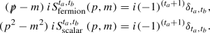  (A.1)

  Henceforth we shall suppress the subscript of scalar or fermion since the context will be clear. We shall also use the compressed notation, $i{S}^{t_a,t_b}(p,m) \equiv i S^{t_a,t_b}_p$.

• 2. The generalised Feynman identities: Consider an nth order graph with s vertices labelled u to 1 from the hard vertex V to the right (see Fig. 7).

  Fermionic case: We now insert the $\mu$ vertex of the $(n+1)$th K photon with momentum k between vertices $q+1$ and q on the $p'$ fermion leg. Here the vertex label codes for both the momentum and the thermal type: the momentum $p'+\sum _{i=1}^{q}l_i$ flows to the left of the vertex q on the $p'$ fermion leg. The photon at this vertex has momentum $l_q$, with Lorentz index $\mu _q$, and thermal type-index $t_q$. Denoting $(p'+\sum _{i=1}^q l_i)$ as $p'+\sum _q$ and using Eq. A.1, we have

  

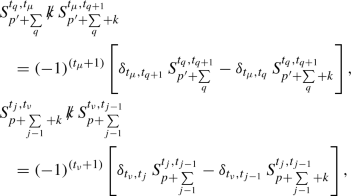  (A.2)

  where the second line corresponds to the GY reduction when a virtual K photon with momentum k is inserted at the vertex $\nu$ to the left of vertex j on the p leg. If the photon vertex is inserted to the right of the vertex labelled ‘1’ on the fermion leg with momentum $p'$, we have

  

  (A.3)

  since , and the second line corresponds to the similar relation that holds for the insertion of the virtual K photon at a vertex $\nu$ on the fermion p leg just to the left of vertex ‘1’, since as well.

  Scalar case: Similarly, for the insertion of a virtual K photon at the vertex $\mu$ to the left of vertex q on the $p'$ scalar leg (insertion of $\nu$ to the left of vertex j on the p leg), we have

  $$\begin{aligned}&S^{t_q,t_\mu }_{p'+\sum \limits _q} \left[ (2p'+2\Sigma _q+k)\cdot k\right] S^{t_\mu ,t_{q+1}}_{p'+\sum \limits _q+k}\nonumber \\&\quad = (-1)^{(t_\mu +1)} \left[ \delta _{t_\mu ,t_{q+1}}\, S^{t_q,t_{q+1}}_{p'+\sum \limits _q} - \delta _{t_\mu ,t_q}\, S^{t_q,t_{q+1}}_{p'+\sum \limits _q+k} \right] , \nonumber \\&S^{t_j,t_\nu }_{p+\sum \limits _{j-1}+k} \left[ (2p+2\Sigma _{j-1}+k)\cdot k\right] S^{t_\nu ,t_{j-1}}_{p+\sum \limits _{j-1}}\nonumber \\&\quad = (-1)^{(t_\nu +1)} \left[ \delta _{t_\nu ,t_j}\, S^{t_j,t_{j-1}}_{p+\sum \limits _{j-1}} - \delta _{t_\nu ,t_{j-1}}\, S^{t_j,t_{j-1}}_{p+\sum \limits _{j-1}+k} \right] , \end{aligned}$$

  (A.4)

  where the $S^{t_q,t_\mu }_{p'+\sum \limits _{q}}$, etc., refer to scalar propagators where the subscript ‘scalar’ has been dropped for clarity. If the photon vertex is inserted to the right of the vertex labelled ‘1’ on the scalar leg with momentum $p'$ (or to the left of vertex ‘1’ on the p leg), we have

  $$\begin{aligned}{}[(2p'+k)\cdot k] \,S^{t_\mu ,t_1}_{p'+k}&= \delta _{t_\mu ,t_1}\, (-1)^{(t_\mu +1)}, \nonumber \\ S^{t_1,t_\nu }_{p+k} \, [(2p+k)\cdot k]&= \delta _{t_\nu ,t_1}\, (-1)^{(t_\nu +1)}, \end{aligned}$$

  (A.5)

  since $p'^2 = p^2 = m^2$.

References

M. Beneke, F. Dighera, A. Hryczuk, JHEP 1410, 45 (2014). arXiv:1409.3049 [hep-ph] [Erratum: JHEP 1607, 106 (2016)]
R.L. Kobes, G.W. Semenoff, Nucl. Phys. B 260, 714 (1985)
A.J. Niemi, G.W. Semenoff, Nucl. Phys. B 230, 181 (1984) See also R.J. Rivers in [4] below
R.J. Rivers, Path Integral Methods in Quantum Field Theory, Chapter 15 (Cambridge University Press, Cambridge, 1987)
H.A. Weldon, Phys. Rev. D 49, 1579 (1994)
J.F. Donoghue, B.R. Holstein, R.W. Robinett, Ann. Phys. 164, 233 (1985)
G. Grammer Jr., D.R. Yennie, Phys. Rev. D 8, 4332 (1973)
D. Indumathi, Ann. Phys. 263, 310 (1998)
P. Sen, D. Indumathi, D. Choudhury, Eur. Phys. J C 79, 532 (2019). arXiv:1812.04247
S. Gupta, D. Indumathi, P. Mathews, V. Ravindran, Nucl. Phys. B 458, 189 (1996)
A. Das, Indian Nat. Sci. Acad. (2000). arXiv:hep-ph/0004125
I. Ojima, Ann. Phys. 137, 1 (1981) Seealso M. Le Bellac in [13] below
M. Le Bellac, Thermal field theory. Cambridge University Press (1996)
A. Das, P. Kalauni, Phys. Rev. D 93, 125028 (2016). arXiv:1605.05165 [hep-th]
A. Denner, H. Eck, O. Hahn, J. Küblbeck, Phys. Lett. B 291, 278 (1992) [See also CERN lecture notes, A. Denner, CERN-TH.6549/92, 1992]
E. Komatsu et al. (WMAP Collaboration), Astrophys. J. Suppl. 192, 18 (2011). arXiv:1001.4538 [astro-ph]
P.A.R. Ade et al. (Planck Collaboration), Astron. Astrophys. 594, A13 (2016). arXiv:1502.01589 [astro.ph]
M. Beneke, F. Dighera, A. Hryczuk, JHEP 1609, 031 (2016). arXiv:1607.03910
Acknowledgements
We thank M. Beneke for bringing the results of Ref. [18] to our attention after reading Ref. [9]. DC acknowledges partial support from the SERB, India, under research grant CRG/2018/00488920 and the European Union’s research and innovation program under Marie Skłodowska-Curie grant No 690575. We thank the referee for a very careful reading of the manuscript which considerably improved the quality of the paper.
Author information
Authors and Affiliations
Corresponding author