
Abstract
Corrosion costs an estimated 3–4% of GDP for most nations each year, leading to significant loss of assets. Research regarding automatic corrosion detection is ongoing, with recent progress leveraging advances in deep learning. Studies are hindered however, by the lack of a publicly available dataset. Thus, corrosion detection models use locally produced datasets suitable for the immediate conditions, but are unable to produce generalized models for corrosion detection. The corrosion detection model algorithms will output a considerable number of false positives and false negatives when challenged in the field. In this paper, we present a deep learning corrosion detector that performs pixel-level segmentation of corrosion. Moreover, three Bayesian variants are presented that provide uncertainty estimates depicting the confidence levels at each pixel, to better inform decision makers. Experiments were performed on a freshly collected dataset consisting of 225 images, discussed and validated herein.
Introduction
Corrosion of steel and other engineering alloys is an ongoing concern for society, as the resulting deterioration can result in significant consequences, environmental damage, and significant financial loss1. In studies that have sought to determine the annual cost arising from corrosion it is usually estimated to be between 3 and 4% of GDP2; with between 15 and 35% of this amount thought to be avoidable, and a significant proportion relating to the cost of inspection3.
Research into automated corrosion detection is driven by cost savings and risk mitigation, with several publications on the subject over the last decade4,5,6,7,8,9, prompted by improvements in deep learning, computer vision and the availability of increasing computing power. A comprehensive review of research into deep learning for materials degradation, including corrosion detection, was carried out and reported by Nash, Drummond and Birbilis10. Previous work by the authors demonstrated the ability of a deep learning model to produce semantic segmentation maps, labelling each pixel of an image as either corrosion, or, background11,12. The current state-of-the-art for corrosion detection trained three model architectures: FCN, U-Net and Mask R-CNN on a private dataset9. Using edge detection to refine the boundaries of detected areas the best performance was reported for the Mask R-CNN model, with an average F1-Score of 0.71.
To date, no labelled corrosion image datasets have been openly published, and the aforementioned models are prone to misclassification of subjects that are not prevalent in the relatively small training set. In the consideration of practical (industrial) utility of deep learning semantic segmentation models to be useful, some measure of prediction uncertainty is required to avert either unnecessary or potentially costly decisions. Herein we deploy three variants of Bayesian deep learning to provide confidence estimates at the pixel level for corrosion detection.
Deep learning model architectures such as LeNet13, AlexNet14, VGG15, DenseNet16 and FCN17 have set benchmarks in competitive computer vision exercises, demonstrating impressive gains in accuracy each year. However, whilst such models are both efficient and have high levels of accuracy, these models do not provide estimates of model uncertainty and fail when the input is not represented in the training set, so called Out of Distribution (OoD) data18,19.
Although the penultimate layer of deep learning models (i.e., the logit layer) is sometimes assumed to represent the probability of detection and thus model uncertainty, these models are optimised on the closed training set to map the input data to the output labels, thus the logit layer outputs cannot be used to provide uncertainty estimates in deployment20.
In a prior study, the authors trained a “Fully-Convolutional-Network” (FCN) model to produce semantic segmentation of corrosion11. After training for 50,000 epochs on a subset of the dataset used herein, this model was only able to achieve an F1-Score of 0.55 (refer to Section “Dataset, evaluation protocol and implementation details” for details on F1-Score). Furthermore, when challenged with images from outside of the training distribution the model was prone to produce false positive detection, notably for faces and foliage. These errors present a significant barrier to deployment, because for decision makers or engineers, knowing the confidence of automatic corrosion detection is essential.
Bayesian neural networks (BNNs) were developed in the 1990s21,22 and have been extended to deep neural networks in recent times, as indicated for example in the following works18,23,24,25,26,27. Bayesian neural networks modify deep learning models by replacing single point weights with distributions, thus producing probabilistic outputs. For Bayesian deep learning the appropriate prior probability distributions of the model’s weights are intractable and are usually taken as a random initialization of the model parameters. Progressive updates of the posterior distributions of weights are achieved through gradient descent, until a satisfactory level of accuracy has been achieved. Thus, Bayesian deep learning is capable of advantageously utilising the tools of deterministic deep learning to provide so-called Bayesian approximation28.
Three available methods to incorporate Bayes methods into classical deep learning models are summarised as follows:
-
Variational inference methods replace a portion of network weights with distributions, typically Gaussian, parameterized by the mean and standard deviation. Data is then fed through the Bayesian neural network multiple times, with the weights of the network drawn from their Gaussian distribution on each forward pass. Shridhar et. al. have provided a straightforward method to modify convolutional neural networks to permit variational inference29.
-
Monte Carlo dropout applies “dropout” during both training and inference, by applying a Bernoulli distribution to the weights, which again requires multiple passes through the network. The application of Monte Carlo dropout was utilised to modify the DenseNet model for Bayesian semantic segmentation of driving scenes obtained from the CamVid and NYUv2 datasets18.
-
The ensemble method utilises multiple models that have been trained from different initializations and therefore are likely to be optimized to different local minima. A recent study summarizes the case for interpreting ensemble models as approximate Bayesian marginalisation; whereby the ensemble model weights are interpreted as sampling from the posterior distribution30.
These Bayesian Deep Learning models can then be used to output not just the predicted class map, but the uncertainty of the prediction. Evaluation of uncertainty is typically categorized as epistemic uncertainty and aleatoric uncertainty. Kendall and Gal explore these two categories of uncertainty in detail for Bayesian deep learning18, with these categories also utilised in reported works25,29,30. However, there is no distinct definition of what constitutes and differentiates the so-called epistemic and aleatoric uncertainty. Epistemic uncertainty is commonly ascribed to model uncertainty31,32, with the understanding that a deep learning model can only be trained on a closed set that is itself a subset of the universal open set (i.e., all data in the universe). As the size of the training set increases, epistemic uncertainty should decrease.
Conversely, aleatoric uncertainty is related to the inherent noise of the input signal. Resolving aleatoric uncertainty requires somehow modifying the input, e.g., increasing resolution, illuminating areas, or capturing the data (image) from multiple angles. Obviously, for any input already captured, the aleatoric uncertainty cannot be reduced. Ideally, each input image will produce the same aleatoric uncertainty regardless of the model, although in Bayesian deep learning the aleatoric uncertainty estimation is dependent on the model.
Results and discussion
Accuracy of the Bayesian variants
The mean Intersection of Union (mIoU) and F1-Score are used to assess the accuracy of prediction, these are standard metrics for semantic segmentation tasks derived from the True Positives (TP), True Negatives (TN), False Positives (FP) and False Negatives (FN) as follows:
Figure 1 illustrates these metrics, as the overlap between label and prediction improves the mIoU and F1-Score will approach one. F1-Score is preferred for subjects that have a class imbalance between the target (in this instance, corrosion) and background, because the F1-Score has a higher weighting for True Positives (TP).

The top-right circle is the ground truth, and bottom right is the prediction, then the True Positive is shown in white, True Negative in Black, False Positive in Cyan, and False Negative in Red.
Train and test F1-Scores for the variational, Monte-Carlo dropout and ensemble models during tenfold cross-validation training are plotted in Figs. 2, 3 and 4 respectively—the raw model output is shown as well as the aleatoric adjusted output, note that the epistemic output was not evaluated during training. The minimum, maximum and average test F1-Scores (raw and adjusted) for each model are summarized in Table 1, the F1-Score achieved on a subset of the current dataset in11 is provided for comparison. It is stressed that it was not the principal intent of this study to produce highly accurate models (instead, the purpose was to produce models that can provide uncertainty estimates). For comparison the state-of-the-art for semantic segmentation of corrosion is reported to achieve an F1-Score of ~0.719. Testing was performed on the best performing model based on the F1-Score of the uncertainty adjusted output, in the case of the ensemble model the best performing checkpoint from each fold was used, forming an ensemble of nine models (the last fold was discarded because it terminated early).

F1-Scores evaluated on the training and test sets during tenfold cross-validation training.

F1-Scores evaluated on the training and test sets during tenfold cross-validation training.

F1-Scores evaluated on the training and test sets during tenfold cross-validation training (note that the training was terminated due to a power outage on the last fold after 75 epochs).
Figure 5 shows five example input images from the test set with their corresponding ground truth label maps. The output corrosion maps and accuracy maps of the example input images (Fig. 5) are presented for the variational model in Fig. 6, the Monte-Carlo dropout model in Fig. 7 and the ensemble model in Fig. 8. The accuracy maps are produced by overlaying the corrosion prediction maps with the ground truth map, following the schema presented in Fig. 1. These accuracy maps are output only when a ground-truth label map is provided during inference.

Images (first and third rows), with their corresponding ground truth label maps (second and fourth rows), red = corrosion, black = background.

The corrosion detection output (first and third row) and accuracy maps (second and fourth row) from the variational model of the input and ground truth label maps shown in Fig. 5. Detection colour determined by output layer confidence, cyan is higher.

The corrosion detection output (first and third row) and accuracy maps (second and fourth row) from the Monte-Carlo dropout model of the input and ground truth label maps shown in Fig. 5. Detection colour determined by output layer confidence, cyan is higher.

The corrosion detection output (first and third row) and accuracy maps (second and fourth row) from the ensemble model of the input and ground truth label maps shown in Fig. 5. Detection colour determined by output layer confidence, cyan is higher.
Epistemic and aleatoric uncertainty
The epistemic and aleatoric uncertainty maps are presented in Fig. 9 for the variational model, Fig. 10 for the Monte-Carlo dropout model and Fig. 11 for the ensemble model. High uncertainty is yellow, and low uncertainty is purple. The plots of F1-Score vs threshold for the training dataset images are shown in Fig. 13.

The epistemic (first and third row) and aleatoric (second and fourth row) uncertainty maps produced by the variational model for the example input images (Fig. 5). Colour scaled from low = purple to high = yellow.

The epistemic (first and third row) and aleatoric (second and fourth row) uncertainty maps produced by the Monte-Carlo dropout model for the example input images (Fig. 5). Colour scale from low = purple to high = yellow.

The epistemic (first and third row) and aleatoric (second and fourth row) uncertainty maps produced by the ensemble model for the example input images (Fig. 5). Colour scale from low = purple to high = yellow.
To compare the performance of the models developed herein with test images from outside of the domain (OoD) of the training set, a novel dataset was collated and labelled of 14 corrosion images from distinctly different settings. Example results from the novel dataset are provided in:
-
Figure 12: a corroded truss column and brace,
Fig. 12: Bridge column image and model outputs. 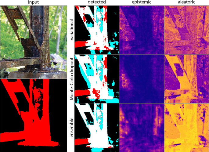
Example from Out of Distribution set: Left panel: input image and ground truth label map; Right panel: top row: variational model outputs, middle row: Monte-Carlo dropout model outputs; bottom row: ensemble model outputs; left column: detection maps; middle column: epistemic uncertainty; right column: aleatoric uncertainty.
-
Supplementary Fig. 1: corroding exhaust vents from an industrial setting, and
-
Supplementary Fig. 2: a person inspecting the abutment of a corroded bridge, with foliage in the background.

The novel dataset images were labelled to allow evaluation of the F1-Score achieved from the raw model and the impact of uncertainty on the model accuracy.
F1-Scores for each of the input images are provided in Table 2, measured with a fixed threshold of 0.75. These results show the performance difference for images with concentrated corrosion that is well lit (e.g., Fig. 5a. through 5e.), compared to images with fine details small and dispersed corrosion, that are overexposed or in shadow (e.g., Fig. 5f. through 5j.)
A summary of the maximum uncertainties output from the models for the inputs shown is provided in Supplementary Table 1.
Uncertainty metrics
F1-Score vs Threshold plots were evaluated on the training dataset (Fig. 13) and the novel dataset (Fig. 14), these show the effect of adjusting for uncertainty on the F1-Score as the threshold is increased from 0 to 1.

Left: variational; middle: Monte-Carlo dropout; right: ensemble.

Left: variational; middle: Monte-Carlo dropout; right: ensemble.
Individual F1-Score vs. Threshold plots for two individual images from the training set (Fig. 5e and h) are shown in Fig. 15, these illustrate how the optimum threshold can vary from image to image, and the influence of the number of positive pixels in the label, for instance the small area of corrosion in Fig. 5h provides a narrow range of good thresholds.

Top row: variational model; middle row: Monte-Carlo dropout model; bottom row: ensemble model.
Sparsity curves were also measured and are presented for the training dataset in Fig. 16 and for the novel dataset in Fig. 17. These show the effect of removing pixels progressively from the error calculation (in this case the root mean square error), and compare the uncertainty outputs against the “oracle” of binary-cross-entropy-loss.

Left: variational; middle: Monte-Carlo dropout; right: ensemble.

Left: variational; middle: Monte-Carlo dropout; right: ensemble.
Bayesian models vs. human performance
The results presented herein (Table 1) demonstrate that for all three model variants the accuracy of corrosion detection approaches and even exceeds what may be considered human accuracy on the dataset, if taking the estimated F1-Score of 0.81 from analysis of human labelling of the MS-COCO dataset as a benchmark33. Based on the average F1-Score achieved during the test phase of tenfold cross validation each model exceeds best in class accuracy of 0.71 F1-Score, although it must be noted that a fair comparison requires that the models are tested on the same dataset—currently this is not possible due to restrictions placed on the respective datasets – it is considered likely that the models presented herein would have low accuracy when challenged with the dataset used in9. Previous work by the authors estimated that a minimum dataset size of at least 9,000 images is required to approach human accuracy11, ideally taken from a wide variety of settings. Considering the training set is roughly 3% of this figure (of 9000), the accuracy achieved is impressive. Moreover, the incidence of false-negatives is less common than false-positives, which is desirable for decision makers, who would rather the model detect corrosion where there is none than miss corrosion.
It is postulated herein that corrosion is a difficult target for computer vision because it does not have common shape-based features and varies in colour; for steels it is most often a dull red, but can be black, vibrant orange, and even green. Corrosion falls under the “stuff” cohort of subjects along with “the sky”, “the sea”, “carpet”, etcetera; contrasted with “things” like cats and dogs that are discrete and have distinct shape based features34. Things can be defined by their shapes in a way that stuff cannot, convolution filters used in deep learning models are well suited for detecting shape based features35 and these models are more successful detecting things than stuff. In 2017 and 2018 MS COCO ran the stuff segmentation challenge with 91 classes (corrosion was not included), the leading model achieved an average mean-intersection-of-union (mIoU, refer to Section “Prediction, epistemic and aleatoric uncertainty”) of just 0.29436. Since then the panoptic challenge was implemented to segment both stuff and each instance of things in images, the current leading model records F1-Scores of 0.746 for things but just 0.488 for stuff37.
For all models, prediction of corrosion in the OoD set returns false-positives for foliage, water, and text (either from in-image signage or from timestamps). This may be expected on the basis that the model has not encountered these subjects during training. Expanding the training set to include these subjects is expected to improve performance when they are encountered during test time. However, in the absence of a universal training set, it is important that the user of the models can judge model certainty for these predictions. All models also make false detections where the lighting conditions are markedly different from the training set.
It is noted that the variational and Monte-Carlo dropout models will produce different predictions for every inference of the same image, because they are effectively drawing model weights from their respective Gaussian and Bernoulli distributions. Conversely, the ensemble models’ weights are deterministic, and for any given image the model will always produce the same output.
Evaluation of epistemic uncertainty
Across all three models the epistemic uncertainty is distinctly lower in the true positive regions. There is significant variation in the quality of the epistemic uncertainty maps, with the ensemble method providing clear outputs, while the dropout and variational methods are distorted. The epistemic uncertainty maps for the variational model tends to concentrate at the edges of the detected corrosion, whereas Monte-Carlo dropout and ensemble epistemic uncertainty maps primarily highlight the background / not corrosion areas. In terms of quality the Monte-Carlo dropout model produces noticeable orthogonal banding in the epistemic uncertainty, while the ensemble model output for epistemic uncertainty retains fine detail. Based on the results shown in Supplementary Table 1, generally the epistemic uncertainty was found to be higher for the novel dataset compared to the training dataset, therefore the maximum epistemic uncertainty could be used as a pseudo-confidence level for decision makers.
Evaluation of aleatoric uncertainty
For all Bayesian variants the aleatoric uncertainty maps are higher in shadows, overexposed areas, dark paint, and unclear areas of the images. The aleatoric uncertainty is also higher in corroded areas, this may be due to the model learning to “hedge its bets”, but is also likely due to corrosion presenting as darker regions of images. In the context of asset inspection, the aleatoric uncertainty is less critical, but can inform decision makers about locations that need closer inspection or improved image capture. As expected, the aleatoric uncertainty maps are largely consistent across the methods, other than differences in contrast; ideally aleatoric uncertainty is input dependant and will not vary from model to model.
Optimal threshold and uncertainty adjustment
To test the value of the uncertainty estimates the outputs were adjusted and measured for F1-Score vs threshold and sparsity plots were generated. The aleatoric uncertainty was recovered using Eq. (4), however the epistemic adjustment was made simply by subtracting the standard deviation from the mean of the output. Note that when tested against the entire training set the average F1-Score performance is lower than achieved during training, because during k-fold cross validation training the model is tested against a subset of the entire dataset which changes on each fold.
The threshold chosen has a strong influence on the accuracy of segmentation, and the optimum threshold varies from image to image. In deployment the optimum threshold is unknown, and we see for example in Fig. 5h that the F1-Score at our chosen threshold of 0.75 is much lower than if we had selected a threshold of 0.9 as shown in the F1-Score vs Threshold curve in Fig. 15. We also observe that the optimum threshold is reduced for the novel dataset (Fig. 14) when compared to the training dataset (Fig. 13).
When tested on the images from within the training distribution adjusting for the epistemic uncertainty shifts the optimal threshold and effects the maximum F1-Score, positively for the Monte-Carlo dropout and ensemble models but negatively for the variational model (Fig. 13). When challenged with novel images from outside the training distribution a similar effect is seen, whereby adjusting for epistemic uncertainty reduces the optimal threshold, but in this case it reduces the maximum F1-Score for every model (Fig. 14). On the other hand, the adjusting for aleatoric uncertainty increases the F1-Score across a wider range of thresholds for the ensemble model and Monte-Carlo model but is overall not influential to the variational model performance.
When the optimum threshold is unknown (i.e., during deployment) the aleatoric uncertainty for the Monte-Carlo dropout and Ensemble model will usually increase the F1-Score. Interestingly, the sparsity plots (Figs. 16 and 17) suggest that the epistemic uncertainty tracks more closely to the oracle, although it is less influential on the F1-Scores.
Prospects
To improve model accuracy, one obvious key task should be increasing the size of the expertly labelled dataset. Crowdsourced recruiting of experts to label images for classification has been successful thanks to self-selection bias38, and this approach could be extended to semantic segmentation. Extending the dataset to other defects such as paint blisters, delamination, and peeling, may also be expected to also improve accuracy - since more information is encoded in the model weights, enabling finer segmentation of input images. In the absence of a universal dataset, it may be necessary to create datasets for specific settings where models will be deployed, i.e., localised datasets for specific regions or contexts.
The work herein demonstrates three measures to transform deep learning networks into deep Bayesian networks. Aleatoric and epistemic uncertainties provide operators with useful information about the confidence of prediction, and which areas need to be inspected more closely. In terms of performance the ensemble method is found to be the most informative for decision makers and achieves the highest segmentation accuracy. This is important to the utilisation of deep learning as an engineering tool. Furthermore, it is advantageous that the ensemble method will always produce the same output for each inference run. By combining models trained to different optimisations, this method presents opportunities to explore different training regimes, including pre-training on disparate datasets, which may improve the accuracy in unfamiliar settings.
Finally, further work is recommended to explore additional signal capture techniques, such as infrared imaging, that can provide additional information for making decisions and may also alleviate the issues surrounding false positive corrosion detection (for example, of foliage or people). Other avenues for possible improvements include multi-task learning to combine so called “stuff” (e.g., “corrosion”, “paint”, “sky”, “grass”) and “things” (e.g., “pipe”, “valve”, “tree”, “car”), this measure is known to improve performance of both tasks, as information is shared between the model branches39.
Methods
Model architecture
In the present work, the base deep learning model is the High-Resolution Network as modified for sematic segmentation (HRNetV2), which has achieved state-of-the-art results on the public datasets of Cityscapes, PASCAL and MS COCO40. The HRNetV2 code and weights pre-trained on the MSCOCO Stuff dataset41 are available online at https://github.com/HRNet/HRNet-Semantic-Segmentation. HRNetV2 consists of four parallel branches with progressively smaller resolutions, which are upsized to full resolution and concatenated to produce the label maps, this architecture is shown in Fig. 18.

Schematic of the base model of the HRNetV2 architecture utilized herein.
Modifying HRNetV2 in three different configurations provides the Bayesian variants:
-
1.
Variational inference: At the end of each branch a variational convolution layer was inserted with separate μ and σ parameters used to sample from the normal distribution for the convolution kernel weights on each forward pass.
-
2.
Monte Carlo dropout: In-line dropout is applied at the end of each branch, effectively placing a Bernoulli distribution over the branches during both training and inference.
-
3.
Ensemble: HRNetV2 was trained multiple times to provide an ensemble of models optimized to different local minima. During inference the input is run through each of the models and the mean and standard deviation of the outputs is used to estimate uncertainty.
Following the work of Kendall and Gal18, each of the three variants described above was modified to provide an additional output: the “aleatoric” uncertainty map, which is treated as the log variance. The binary cross entropy loss function was adapted as shown in Eq. (3) to train the model to output the predictions of corrosion and the “aleatoric” uncertainty, which we term “Bayesian binary-cross-entropy”:
where D is the number of pixels in the image, si is the log variance (\(\log _e\hat \sigma ^2\)), yi and \(\hat y_i\) are the pixel label and prediction respectively. This loss trains the model to output the predictions of corrosion alongside the “aleatoric” uncertainty.
Dataset, evaluation protocol and implementation details
The training set utilised herein is comprised of 225 images of corrosion that were taken from an industrial site, such that the study has practical relevance. The images (photos) that comprise the dataset were captured by consumer camera (digital SLR) in the visible light spectrum, supplied as compressed jpegs, and vary in resolution from 50,496 to 36,329,272 pixels. Supplementary Figure 3 plots the image dimensions and Supplementary Figure 4 shows a stacked histogram of the dataset red-green-blue spectrums which provides an indication of the characteristics of the dataset distribution.
Each image was expertly labelled and provided with a ground truth image comprising per-pixel labelling of “corrosion” and “background”. Due to the small dataset size k-fold cross validation was used for training with 10 folds.
Weights from HRNetV2 pretrained on the MS-COCO Stuff dataset41 were used to initialize the model at the start of each training fold. Model weights that were not present in the pretrained HRNetV2 model such as the aleatoric branch or the gaussian parameters of the variational convolutional layers were initialized randomly from the normal distribution. Using pretrained model weights on a new task is termed “transfer learning” and reduces training time significantly because the lower-level weights are already trained to detect relevant features. The MS COCO Stuff dataset was chosen because “corrosion” is also considered to be “stuff” that has no fixed shape and is not found in clearly discrete instances (compared to things, which are discrete with fixed shapes).
Training hyperparameters were selected based on past trial and error to achieve good accuracy on the dataset within 200 epochs. The learning rate was set to 0.0001, and trained using the RMSProp optimizer; thus following Gal and Ghahramani who demonstrate that this schema effectively minimizes the Kullback-Leibler (KL) divergence between the approximate distribution and the full posterior42. During each fold the models were trained for 80 epochs using the standard binary-cross-entropy loss, after which the loss function switched to the Bayesian binary-cross-entropy (Eq. (3)) for a further 40 epochs for the Monte-Carlo dropout and ensemble models, and a further 70 epochs for the variational model. At every 10th epoch the model was validated against the fold test set, and a checkpoint saved which can be loaded for evaluation later. The code was written using the PyTorch® deep learning framework and is available at https://github.com/StuvX/SpotRust.
Prediction, epistemic and aleatoric uncertainty
During inference the input image is passed forward through the modified HRNetV2 model N times, the outputs are then stacked to provide an array of shape [N, C, H, W] and the prediction is taken as the mean of the stochastic outputs of the model. We use a threshold of 0.75 of the output, above which the pixel is labelled “corrosion”, otherwise it is labelled “not corrosion”.
The modified HRNetV2 models herein also output a log variance map of model uncertainty that is interpreted as the aleatoric uncertainty. Again, the Bayesian outputs are stacked and the aleatoric uncertainty is taken as the mean of the stack. The epistemic uncertainty is then taken as the variation of the model output stack, intuitively this captures the (dis)agreement of the stochastic outputs.
To evaluate the benefit of the uncertainty outputs the F1-Score is also calculated with the outputs adjusted for uncertainty. This adjustment is calculated according to Eq. (4) to recover the prediction with uncertainty (notation per Eq. (3)). Each model was tested against the training set and novel set by measuring the “F1-Score vs threshold” based on the raw model output and adjusted uncertainty outputs as the threshold is increased from 0 to 1.
Sparsity plots were also evaluated using the method described in25. These plots compare the effect of removing pixels from the evaluation on the normalized mean-squared-error. Pixels are progressively removed from highest uncertainty to lowest, and compared against the “oracle”, taken as the binary-cross-entropy loss between the model output and the ground truth label. An ideal uncertainty metric should closely follow the “oracle” sparsity plot.
Data availability
The corrosion dataset may be made available subject to controlled access due to legal requirements, please contact the corresponding author.
Code availability
Code and trained model files are provided at https://github.com/StuvX/SpotRust.
References
Hansson, C. M. The impact of corrosion on society. Metall. Mater. Trans. A Phys. Metall. Mater. Sci. 42, 2952–2962 (2011).
Hou, B. et al. The cost of corrosion in China. npj Mater. Degrad. 1, 4 (2017).
Koch, G. et al. International Measures of Prevention, Application, and Economics of Corrosion Technologies Study. NACE Int. 1–3 (2016).
Yammen, S. & Muneesawang, P. An Advanced Vision System for the Automatic Inspection of Corrosions on Pole Tips in Hard Disk Drives. IEEE Trans. Components. Packag. Manuf. Technol. 4, 1523–1533 (2014).
Liu, L., Tan, E., Yin, X. J., Zhen, Y. & Cai, Z. Q. Deep learning for Coating Condition Assessment with Active perception. in Proceedings of the 2019 3rd High Performance Computing and Cluster Technologies Conference 75–80 (ACM, 2019).
Bonnin-Pascual, F. & Ortiz, A. Corrosion Detection for Automated Visual Inspection. in Developments in Corrosion Protection 619–632 (InTech, 2014).
Jiang, J., Wang, Z., Guo, H. & Cheng, J. Multiresolution Analysis Driven Corrosion Detection on Metal Surface. in 2011 International Conference on Multimedia and Signal Processing 85–88 (IEEE, 2011).
Petricca, L., Moss, T., Figueroa, G. & Broen, S. Corrosion Detection Using A.I.: A Comparison of Standard Computer Vision Techniques and Deep Learning Model. in Computer Science & Information Technology (CS & IT) 91–99 (Academy & Industry Research Collaboration Center (AIRCC), 2016).
Katsamenis, I., Protopapadakis, E., Doulamis, A., Doulamis, N. & Voulodimos, A. Pixel-Level Corrosion Detection on Metal Constructions by Fusion of Deep Learning Semantic and Contour Segmentation. in Lecture Notes in Computer Science (including subseries Lecture Notes in Artificial Intelligence and Lecture Notes in Bioinformatics) 160–169 (2020).
Nash, W., Drummond, T. & Birbilis, N. A review of deep learning in the study of materials degradation. npj Mater. Degrad. 2, 37 (2018).
Nash, W., Drummond, T. & Birbilis, N. Deep Learning AI for Corrosion Detection. in CORROSION 2019 (ed. NACE International) (2019).
Nash, W., Holloway, L., Drummond, T. & Birbilis, N. Artificial Intelligence Assisted Condition Assessment. Corros. Mater. February, 80–83 (2018).
Le Cun, Y. et al. Handwritten digit recognition: applications of neural network chips and automatic learning. IEEE Commun. Mag. 27, 41–46 (1989).
Krizhevsky, A., Sutskever, I. & Hinton, G. E. ImageNet classification with deep convolutional neural networks. Commun. ACM 60, 84–90 (2017).
Simonyan, K. & Zisserman, A. Very Deep Convolutional Networks for Large-Scale Image Recognition. in 3rd International Conference on Learning Representations, Conference Track Proceedings (eds. Bengio, Y. & LeCun, Y.) (2015).
Huang, G., Liu, Z., Van Der Maaten, L. & Weinberger, K. Q. Densely Connected Convolutional Networks. in 2017 IEEE Conference on Computer Vision and Pattern Recognition (CVPR) vols 2017-Janua 2261–2269 (IEEE, 2017).
Long, J., Shelhamer, E. & Darrell, T. Fully convolutional networks for semantic segmentation. in 2015 IEEE Conference on Computer Vision and Pattern Recognition (CVPR) 3431–3440 (IEEE, 2015).
Kendall, A. & Gal, Y.. What Uncertainties Do We Need in Bayesian Deep Learning for Computer Vision? in Advances in Neural Information Processing Systems vols 2017-Decem 5575–5585 (Neural information processing systems foundation., 2017).
Hendrycks, D., Zhao, K., Basart, S., Steinhardt, J. & Song, D. Natural Adversarial Examples. in 2021 IEEE/CVF Conference on Computer Vision and Pattern Recognition (CVPR) 15257–15266 (IEEE, 2021).
Pearce, T., Brintrup, A. & Zhu, J. Understanding Softmax Confidence and Uncertainty. Preprint at http://arxiv.org/abs/2106.04972 (2021).
MacKay, D. J. C. A practical Bayesian framework for backpropagation networks. Neural Comput 4, 448–472 (1992).
Neal, R. M. Bayesian learning for neural networks. Journal of the American Statistical Association vol. 118 (Springer New York, 1996).
Khan, M. E. et al. Fast and Scalable Bayesian Deep Learning by Weight-Perturbation in Adam. in Proceedings of the 35th International Conference on Machine Learning (eds. Dy, J. & Krause, A.) (PMLR, 2018).
Osawa, K. et al. Practical deep learning with Bayesian principles. in Proceedings of the 33rd International Conference on Neural Information Processing Systems vol. 32 (Curran Associates Inc., 2019).
Gustafsson, F. K., Danelljan, M. & Schon, T. B. Evaluating Scalable Bayesian Deep Learning Methods for Robust Computer Vision. in 2020 IEEE/CVF Conference on Computer Vision and Pattern Recognition Workshops (CVPRW) 1289–1298 (IEEE, 2020).
Kendall, A., Badrinarayanan, V. & Cipolla, R. Bayesian SegNet: Model Uncertainty in Deep Convolutional Encoder-Decoder Architectures for Scene Understanding. in Procedings of the British Machine Vision Conference (BMVC) (eds. Kim, T. K., Zafeiriou, S., Brostow, G. & Mikolajczyk, K.) 57.1-57.12. (BMVA Press, 2017).
Khan, M. E. & Rue, H. The Bayesian Learning Rule. Preprint at http://arxiv.org/abs/2107.04562 (2021).
Blundell, C., Cornebise, J., Kavukcuoglu, K. & Wierstra, D. Weight Uncertainty in Neural Networks. in Proceedings of the 32nd International Conference on Machine Learning vol. 37 1613–1622 (JMLR, 2015).
Shridhar, K., Laumann, F. & Liwicki, M. A Comprehensive guide to Bayesian Convolutional Neural Network with Variational Inference. Preprint at http://arxiv.org/abs/1901.02731 (2019).
Wilson, A. G. The case for Bayesian deep learning. Preprint at http://arxiv.org/abs/2001.10995 (2020).
Chen, X., Park, E.-J. & Xiu, D. A flexible numerical approach for quantification of epistemic uncertainty. J. Comput. Phys. 240, 211–224 (2013).
Jakeman, J., Eldred, M. & Xiu, D. Numerical approach for quantification of epistemic uncertainty. J. Comput. Phys. 229, 4648–4663 (2010).
Lin, T.-Y. et al. Microsoft COCO: Common Objects in Context. in Lecture Notes in Computer Science (including subseries Lecture Notes in Artificial Intelligence and Lecture Notes in Bioinformatics) vol. 8693 LNCS 740–755 (2014).
Caesar, H., Uijlings, J. & Ferrari, V. COCO-Stuff: Thing and Stuff Classes in Context. in 2018 IEEE/CVF Conference on Computer Vision and Pattern Recognition 1209–1218 (IEEE, 2018).
Yosinski, J., Clune, J., Nguyen, A., Fuchs, T. & Lipson, H. Understanding Neural Networks Through Deep Visualization. In Deep Learning Workshop, 31st International Conference on Machine Learning 12 (2015).
Kirillov, A., Girshick, R., He, K. & Dollar, P. Panoptic Feature Pyramid Networks. in 2019 IEEE/CVF Conference on Computer Vision and Pattern Recognition (CVPR) vols 2019-June 6392–6401 (IEEE, 2019).
Wang, S. et al. Joint COCO and Mapillary Workshop at ICCV 2019: Panoptic Segmentation Challenge Track Technical Report: Explore Context Relation for Panoptic Segmentation. in ICCV Workshop 2–4 (2019).
Nash, W. T., Powell, C. J., Drummond, T. & Birbilis, N. Automated corrosion detection using crowdsourced training for deep learning. Corrosion 76, 135–141 (2020).
Dharmasiri, T., Spek, A. & Drummond, T. Joint prediction of depths, normals and surface curvature from RGB images using CNNs. in 2017 IEEE/RSJ International Conference on Intelligent Robots and Systems (IROS) 1505–1512 (IEEE, 2017).
Sun, K. et al. High-resolution representations for labeling pixels and regions. Preprint at http//arxiv.org/abs/1904.04514 (2019).
Deng, J. et al. ImageNet: A large-scale hierarchical image database. in 2009 IEEE Conference on Computer Vision and Pattern Recognition 248–255 (IEEE, 2009). https://doi.org/10.1109/CVPRW.2009.5206848.
Gal, Y. & Ghahramani, Z. Bayesian convolutional neural networks with bernoulli approximate variational inference. Preprint at http://arxiv.org/abs/1506.02158 (2015).
Acknowledgements
We gratefully acknowledge support from WSP. This research did not receive any specific grant from funding agencies in the public, commercial, or not-for-profit sectors.
Author information
Authors and Affiliations
Contributions
W.N.—conceptualization, methodology, data curation, software, investigation, original and final draft preparation. L.Z.—conceptualization, methodology, review of manuscript. N.B.—conceptualization, methodology, review of manuscript.
Corresponding author
Ethics declarations
Competing interests
The authors declare no competing interests.
Additional information
Publisher’s note Springer Nature remains neutral with regard to jurisdictional claims in published maps and institutional affiliations.
Supplementary information
Rights and permissions
Open Access This article is licensed under a Creative Commons Attribution 4.0 International License, which permits use, sharing, adaptation, distribution and reproduction in any medium or format, as long as you give appropriate credit to the original author(s) and the source, provide a link to the Creative Commons license, and indicate if changes were made. The images or other third party material in this article are included in the article’s Creative Commons license, unless indicated otherwise in a credit line to the material. If material is not included in the article’s Creative Commons license and your intended use is not permitted by statutory regulation or exceeds the permitted use, you will need to obtain permission directly from the copyright holder. To view a copy of this license, visit http://creativecommons.org/licenses/by/4.0/.
About this article

Cite this article
Nash, W., Zheng, L. & Birbilis, N. Deep learning corrosion detection with confidence. npj Mater Degrad 6, 26 (2022). https://doi.org/10.1038/s41529-022-00232-6
Received:
Accepted:
Published:
DOI: https://doi.org/10.1038/s41529-022-00232-6
- Springer Nature Limited
This article is cited by
-
Data-driven machine learning approaches for predicting permeability and corrosion risk in hybrid concrete incorporating blast furnace slag and fly ash
Asian Journal of Civil Engineering (2024)
-
HEU-Net: hybrid attention residual block-based network with external skip connections for metal corrosion semantic segmentation
The Visual Computer (2024)