
Abstract
Co-catalyst has several roles in propylene polymerization such as site activation, chain transfer, site transformation and Poisson deactivation (or Poisson scavenger). These functionalities strongly impact the most important of the final product properties indices namely the number and weight average. Molecular weight, polydispersity index, melt flow index and even the yield of Ziegler–Natta catalyst. Therefore, the Co-catalyst role as an independent process variable should be carefully investigated in the polymerization. In this study, investigating the co-catalyst effects on the final properties indices and the yield of the catalyst as the existing gap was defined as the aims of this study. We attempt to reply to the problems in a proper way in the absence of hydrogen and at the optimal temperature reaction by proposing a newly developed mathematical model. This model was programmed in MATLAB & Simulink software, then was validated by using experimental data. Through the model, the optimal amount of the used co-catalyst could be determined conveniently.
1 Introduction
Co-catalyst, as Ziegler–Natta catalyst site activation agent, has multiple roles in the polymerization such as site transfer agent, chain transfer agent and site deactivation. without paying attention to use the optimal amount of co-catalyst in the recipe of the polymerization gives rise to some undesired events in the polymerization. These unpleased effects decrease profitability and also the quality of the product. Some of these disadvantages can be described as follows:
Firstly, expected, using less than optimal co-catalyst amount in the formulation of the polymerization makes a large percentage of the catalyst sites remain in the inactivated mood and also the existing poison in the feed, i.e. monomer, stay in the reactor which causes to deactivation the activated sites on the catalyst. Therefore under such circumstances, the consumption of the catalyst increases dramatically.
Secondly, in such a situation, a large amount of the catalyst would be kept inactivated and idle in the reactor. Consequently, the yield of the used catalyst is reduced prominently; and due to the high price of the Ziegler–Natta catalyst, clearly foreseen the product cost would be climbed significantly.
Thirdly, according to Possible co-catalyst reactions in the polymerization, it could be anticipated easily that the co-catalyst has a direct effect on Morphology and Rheology of the polymer and also the performance of the used catalyst; and these important features of the final product and the catalyst performance might be explained by their vital indices namely Poly Dispersity Index (Đ), Melt Flow Index (MFI) and the yield (Y) of the catalyst respectively.
Because of these significant issues, Co-catalyst as an important process variable should be exactly investigated and optimally utilized in the polymerization formulation. So far, few researchers have focused on the problems and remained them as the existing gap; and even despite more than 60 years of using Ziegler–Natta catalyst in polypropylene production, its performance is still unknown. Because its performance entirely depends on the performance of the kinetics of the polymerization in the presence of Ziegler–Natta catalysts; therefore the performance of co-catalyst remains quite complex [1, 2] and the existing gap in this field. Up to now, to determine the amount of the co-catalyst in the polymerization formulation is used by trial and error manner; obviously, this method has a significant error and not reliable in common because it heavily depends on the test and laboratory conditions, the type and the used catalyst system which have a strong impact on its performance and results. It seems that a validated mathematical model based on the kinetic polymerization would be a suitable and reliable way of interpreting the Co-catalyst performance and obtaining optimal co-catalyst amount and to cover the existing gap as well.
The main advantages of using a mathematical model are easy to generate a new grade product, to predict its final properties and formulation in an optimum mode without any hazard. Besides, due to the diversity of the unique catalyst kinetics and chemical substances in polypropylene; in practice, the model gives a profound sense about polymerization, and also it is useful when wanted to apply an unknown and new catalyst to generate a modified recipe according to it.
In this research, we attempted to investigate these issues to cover the existing gap by using a mathematical model and comparing its outputs with an experimental result at the optimal temperature reaction, i.e. 70 °C, in absence of hydrogen [3].
Some experimental researches have been implemented in the field of kinetics study of the polymerization which their attention was only the effect of hydrogen on the kinetics [4, 5], but the reports of them are vague and even in some cases are contradictory without mentioning to the effect of co-catalyst on the kinetics. For instance, Guastalla and Gianinni conducted an experimental investigation to study the effects of hydrogen on the initial rate and activity of the catalyst. They found that the initial rate increase about 2.5 times in presence of hydrogen in the polymerization reactor [6]. however, Spitz et al. claimed that the rate profile of the polymerization is enhanced when low hydrogen concentrations entering the reactor; while at higher hydrogen concentration causes to decrease the catalyst activity and increase the rate of deactivation of the used catalyst [7]. In the opposite, Soga, and Siona reported that the profile rate of the polymerization drops when increased hydrogen amount in the system [8].
Al-haj Ali et al. focused on proposing a generalized model for evaluating hydrogen response in liquid propylene polymerization according to the dormant site [9]. Reginato et al. attempted to justify that a non-ideal continuous stirred tank model can explain an industrial-scale loop reactor [2].
Varshouee et al. performed a computational study by proposing a new validated model based on kinetics study and found that hydrogen has directly impact on final properties so that increasing hydrogen amount in the recipe of the polymerization causes to decreasing of Average Molecular Weights; and also leads to higher activated sites percent on the surface catalyst [3, 10]. They conducted a comprehensive study on Final Product Properties and Kinetics Studies of the polymerization [11,12,13,14] and compared the outputs coming from their model with the experimental results to prove their model and explained the reasons that justify their model was validated [12], then they found that 70 °C is the optimum temperature in their study [3].
Afterward, to be decided which the model would be developed for investigating the co-catalyst effects on indices of the final product properties such as Melt Flow Index, Number, and Weight average molecular weight and Poly Dispersity Index at the optimum temperature, i.e. 70 °C at absence of hydrogen; and also they decided to present how the co-catalyst impacts on the catalytic yield via comparing their improved model outputs with experimental results. In better words, their main targets were to cover the existing gaps as described earlier. This article is the consequences of its decision.
To achieve the defined targets, it was necessary to be developed the previously validated model to be more applicable and fruitful. The selected technique in this model is the polymer moment balance method (population balance approach) which its software has been coded in MATLAB/SIMULINK for slurry polymerization. The implications of this study would be useful for those who work as process engineers in the field of product quality control.
2 Experimental
2.1 Material specifications and experimental polymerization procedure
The used materials and Experimental polymerization procedure are exactly in a similar way that described in detail in the previous works and not repeated here for the sake of brevity [3, 12]. In this study, a commercial catalyst was used.
2.2 Mathematical modeling
2.2.1 Assumptions
In this study, the assumptions for modeling are: (1) It was supposed that propylene polymerization was carried out in the amorphous phase (2) the amorphous phase concentrations during polypropylene polymerization were at the thermodynamic equilibrium condition that obeys the one from Sanchez and Lacombe equation (SLE) [2,3,4,5,6,7,8,9,10,11,12,13,14,15,16,17,18]. (2) It was assumed that γ1 = γ2 = ··· = γNC, where γ is equilibrium constant and NC are several solvents in slurry phase components [2]. (3) The reaction temperature, pressure, and monomer concentration were kept constant during the polymerization process. (4) The resistance of mass and heat transfer and the diffusion effect of the reactants were ignored. (5) It was assumed that the propagation constant is independent of the length of the growing polymer chain. (6) Isothermal reaction and constant monomer concentration during polymerization (7) the deactivation constant follows linearly from the pseudo-first-order which depends on initial polymerization rates [9].
The proposing model in this study is the developed model in the previous works which outlined a new algorithm according to Fig. 1 and entered the co-catalyst reactions in the developed model according to Table 1.

The used algorithm in this study
2.2.2 Mathematical formulas and equations
The mass balance equations [2]:
where Qf feed volumetric flow rate; Q0 reactor-output volumetric flow rate; QR volumetric recirculation flow rate; J components reaction rate, j = 1,2,…,NC.
In this study, Qf and Q0 could be considered “ zero”, because of the process is semi-batch and monomer concentration during the polymerization is constant. Accordingly, the terms of η and ζ are eliminated and meaningless in this study.
The possible reactions of the used co-catalyst in the polymerization are listed in Table 1 which considered in the model of this study. Table 1 shows the co-catalyst reactions that the result of each reaction directly affects on the indices of Morphology and Rheology of the polymer and also the performance of the used catalyst.
The concentration variations with time used in Eq. (1) for modeling are defined as follows:
where k is the site number of the catalyst and CH, CA, CE, CMi, CB, CS, Ccat, and P0 is the concentration of hydrogen, co-catalyst (aluminum alkyl), electron donor, monomer, poison, site transfer, catalyst, and potential site in the polymerization, respectively. It is assumed the first-order reactions for all of the reactions which be reacted in the polymerization [4].
Using the moment equations from Table 2 in Eq. (1) according to the algorithm of this model, i.e. Figure 1 which discussed later in detail, the profile polymerization rate could be explained easily such as Fig. 7.
In many references, other equations could show the rate of polymerization such as Eqs. (2) and (3). These equations are only able to fit the decay part of the profile polymerization rate curve well-known as quasi-steady-state zone [4, 5, 9].
where Rp0 the initial reaction rate (kg gcat−1 h−1]; t time (s); Kd the deactivation constant (l h−1); T reaction temperature (K); Ea,d the activation energy (J/mol); KP the rate constant of the propagation reaction (l mol−1 s−1); C activated site concentration of the catalyst (mol).
Equations (2) and (3) could be used for obtaining Ea and Kd and ultimately for checking validation of the model [12].
To determine Kd and Rp0, it is used by drawing the profile rate of the polymerization in the natural logarithm vs. polymerization time, a linear fit would be obtained in which the slope of the fit line is Kd, and the intercept could be considered as Rp0. By integrating the profile rate of the polymerization, the yield of the used catalyst in the polymerization can be calculated as the following equation in which Ycalc is exactly equal to the area under the profile curve.
The moment equations coming from the population balance approach which used in this study are listed in Table 2.
The model can calculate the final product properties indices of polypropylene by using the moment equations (Population Balance Technique) from Table 2. By the moment equations, the most important indices such as Number average molecular weight (Mn), weight average molecular weight (MW) and polydispersity index (Đ) as final product properties of the polymer would be computed according to the following equations.

The melt flow index (MFI) as the popular Rheology index could be calculated by a power-law-Equation known as the Mark-Houwink model. The constants of the equation should be determined by experimental works. In this study, using the constants obtained from the previous work [10], i.e. a = 9.4841 × 10¹³, b = − 2.3747 in absence of hydrogen in the polymerization.
It is worth emphasized that Eq. (8) only validated in the absence of hydrogen with regarding this study circumstance, it would be suitable. In the presence of hydrogen, in the previous work [13], Eq. (8) is able to predict the melt flow index with a correlation coefficient (R2) of 0.98.
2.2.3 Modelling algorithm
The outlined algorithm in this study is shown in Fig. 1. The computer programming was coded in MATLAB/SIMULINK according to the algorithm of Fig. 1. The proposed model of this study is the developed model of the previous work [3, 12]. In this model, the co-catalyst reaction equations from Table 1 were added to the model and the program is run based on the co-catalyst performance in the polymerization.
By using the iterative method, the kinetic constants are adjusted. Then the necessary steps for validating the model should be done. The iterative method, its algorithm and also the necessary steps for validating a model explained in detail in references 3 and 12 and they are not repeated here for the sake of brevity.
The acceptable proximity of the model outputs with experimental results and their profile rates reveal that the methodology of modeling, i.e. the polymer moment balance method (population balance approach) and also tuning the kinetic constants based on the used catalyst by the iterative method were selected properly in this study. These matters will be explained in the next section, i.e. Results and Discussion.
3 Results and discussion
As mentioned in the introduction, Co-catalyst, as an important process independent variable, has multiple roles such as Ziegler–Natta catalyst site activation agent, site transfer agent, chain transfer agent and site deactivation in the polymerization aaccording to the possible co-catalyst reactions, in the polymerization, as listed in Table 1. As could be anticipated easily from Table 1, the co-catalyst has a direct effect on Morphology and Rheology of the polymer and also the performance of the used catalyst. These important impacts on the final product and the catalyst performance might be explained by their vital indices namely Poly Dispersity Index (Đ), Melt Flow Index (MFI) and the yield (Y) of the catalyst respectively.
Besides, as argued above, the recipe for the polymerization ought to use the optimal amount of co-catalyst. Otherwise, in the polymerization might be happened some undesired events which these events give rise to decrease profitability and the quality of the product. And most importantly, using less than optimal co-catalyst amount in the formulation makes a large percentage of the catalyst sites remain in the inactivated mood and given that under such conditions, there is a shortage of catalysts in the system, the existing poisons in the feed cause to be deactivated the existing activated sites on the catalyst. Therefore expected, the yield of the used catalyst would be reduced dramatically. This happening was observed experimentally.
Accordingly, the problems of this research as the existing gap in this field were revealed:
-
1.
What is the effect of the co-catalyst on Morphology and Rheology of the polymer? In other words, evaluating the impact of the co-catalyst on the final product properties indices, comprising Number and Weight average molecular weight (Mn and Mw), Polydispersity Index (Đ), Melt Flow Index (MFI).
-
2.
What is the effect of the co-catalyst on the catalyst performance, to put it differently, how is the influence of the co-catalyst on the yield of used catalyst?
-
3.
How much is the optimal co-catalyst amount at constant temperature? In this study, the optimum temperature was considered, 70 °C.
To reply to the above research questions, to be concluded a validated mathematical model could be able to cover them properly. In earlier studies attempts were made to establish and propose a validated mathematical model which to be able to show the performance of the polymerization in macro or overall viewpoints [3, 10,11,12,13,14]. In previous work [12], it was scientifically reasoned in detailed how the model will be validated properly with acceptable errors and also discussed and concluded that the selected modeling method, i.e. the polymer moment balance method or population balance approach, could be justified and explained the performance of the polymerization accurately. Obviously, if a kinetic model is able to explain the performance of the reaction properly, then it is easily argued that the used the kinetic constants in the model, to were selected the kinetic constants or fine-tuned appropriately. They are not repeated here for the sake of brevity.
To develop the previous model, the total reactions of the co-catalyst (Table 1) were entered in the algorithm, as shown in Fig. 1. Their kinetic constants were estimated and applied to the model from the iterative method exactly in a similar way that described in detail in the previous works and not repeats here for the sake of brevity [3, 12].
After finished the computer program coding, the same procedure was applied to this newly developed model with different targets, as defined aims earlier in the introduction. In the first, the kinetic constants of all reactions including in this model were fined tuned; then to were taken steps to ensure the validation of the model and to was compared the model outputs with experimental results and was filled Table 3 and compared the experimental with model profile rates as shown Fig. 7. The figure was obtained from Eq. (1) using the moment equation Table 2 according to the designed and proposed in this study. After investigating the model outputs with experimental results as listed in Table 3 and comparing the experimental with model profile rates Fig. 7, due to acceptable proximity among them, the following results were obtained:
-
1.
An appropriate methodology has been chosen for this modeling i.e. the polymer moment balance method (population balance approach).
-
2.
The iterative method is a proper way to fine-tuning the kinetic constants for modeling in this field.
-
3.
The developed model has been validated properly. The acceptable proximity between the model curve and the experimental curve in Figs. 2, 3, 4, 5, 6 and 7 could be considered as other reasons for the validity of the model. Therefore, using this model could be covered the existing gaps and approached to defined aims in this research.
Fig. 2 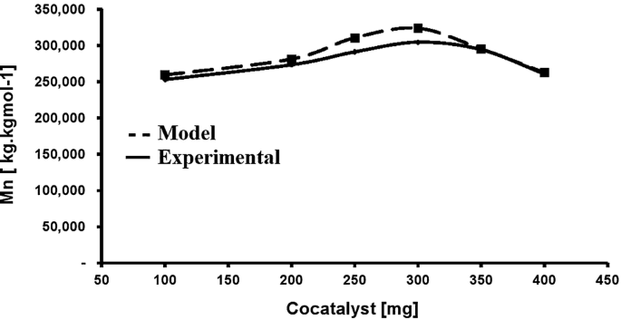
The effect of the co-catalyst amounts on the number average molecular weight (Mn) of the polymer in absence of hydrogen
Fig. 3 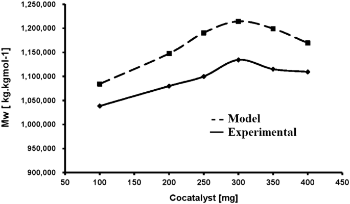
The effect of the co-catalyst amounts on the weight averages molecular weight (Mw) of the polymer in absence of hydrogen
Fig. 4 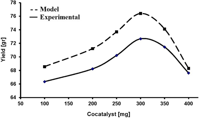
The effect of the co-catalyst amounts on the yield of the used catalyst in the absence of hydrogen
Fig. 5 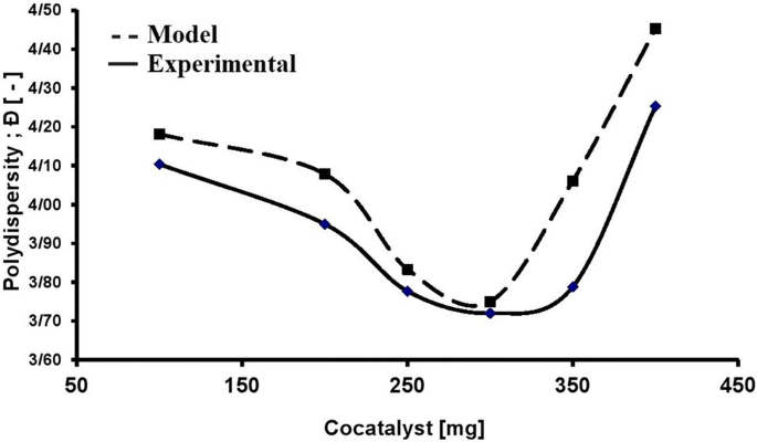
The effect of the co-catalyst amounts on Poly Dispersity Index (Đ) of the polymer in the absence of hydrogen
Fig. 6 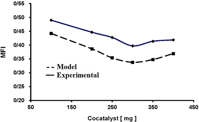
The effect of the co-catalyst amounts on Melt Flow Index (MFI) of the polymer in the absence of hydrogen
Fig. 7 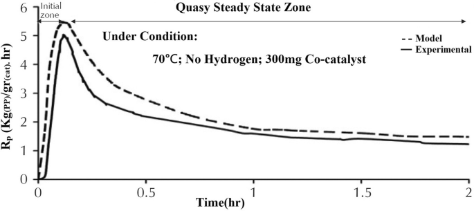
Comparing the experimental with model profile rates in the absence of hydrogen at 300 mg co-catalyst as an optimal condition; i.e. Run 4 from Table 3
-
4.
The existing errors are in the acceptable range.


Due to the existing error is an inherent property of modeling, avoiding error is impossible. The reasons for the error margins could be justified by non-calibrated measurement equipment, personal errors, the numerical calculations, the selected equation of state (EOS) and assumptions.
As mentioned in the introduction and shown possible co-catalyst reactions in the polymerization in Table 1. The co-catalyst has a multilateral role in the polymerization such as Ziegler–Natta catalyst site activation agent; as site transfer agent; chain transfer agent; site deactivation in polypropylene reaction.
To determine the optimal amount of the co-catalyst in the polymerization the following indices should be investigated separately:
-
1.
Molecular weight distribution or poly dispersity index (Đ) as the vital morphology index.
-
2.
Melt Flow Index as the popular Rheology index.
-
3.
the yield of the catalyst as an optimal kinetic index.
According to Eq. (7), poly dispersity index (Đ) is a function of the number average molecular weight (Mn) and weight averages molecular weight (MW) of the polymer. Therefore firstly, it is necessary to be assessed number average molecular weight (Mn) and weight averages molecular weight (MW) of the polymer.
Figures 2, 3, 4, 5 and 6 are plotted according to the data of Table 3 which each of them identifies an important index of the final product properties. These figures show how the variation of the co-catalyst amounts affect directly on the indices. Figures 2 and 3 show the variation of number average molecular weight (Mn) and weight averages molecular weight (MW) of the polymer with the amounts of the used co-catalyst respectively. From the figures, it can be concluded that the maximum amounts of Mn and Mw obtain when used 300 mg co-catalyst in the polymerization formulation. Therefore, 300 mg of the co-catalyst could be considered as one of the reasons that it might be the optimum condition of the recipe, providing that maximum molecular weight of the polymer is desired.
In addition, Figs. 2 and 3 imply the averages molecular weight (Mn and Mw) of the polymer are going up with an increasing co-catalyst, that is to say, lower < 300 mg of co-catalyst. It means that in this area the entered co-catalyst in the reactor is not sufficient to activate all existing sites of the catalyst; in other words, a part of sites on catalyst remains inactive and idle. Therefore, expected that the same behavior would be established the catalyst yield variations with changing co-catalyst amounts in the same circumstance. Figure 4 is affirmed this prediction.
In a kinetic viewpoint, this happening means that the co-catalyst amounts for site activation reaction, i.e. Rxn1 from Table 1, is not enough to react completely; the other existing reactions, rxn2–6 from Table 1, no impact on morphology and rheology of the polymer and can be ignored. Accordingly, to be anticipated that the same trend would have happened for the polydispersity index (Đ) as morphology index and Melt Flow Index (MFI) as a rheology index. Figures 5 and 6 confirmed these expectations on the same range, i.e. below < 300 mg of consuming the co-catalyst in the polymerization.
Commonly, the minimum amount of Polydispersity Index (Đ) is more favored due to the polymer chains are willing to uniformity. From Fig. 5, to be concluded under the situation of 300 mg consuming co-catalyst, the minimum amount of Polydispersity Index (Đ) obtained. This argue as one of the reasons of the optimal condition, could be considered and reasonable.
On the contrary, i.e. above > 300 mg of co-catalyst, all aforementioned behaviors would be reversed which illustrated in Figs. 3, 4, 5 and 6. Consequently, the amount of the used co-catalyst in the polymerization has an optimum amount which 300 mg of co-catalyst could be considered as an optimal point in this study. Therefore, the recipe belongs to Run 4 from Table 3, might be the optimum condition, and its profile rate is shown in Fig. 7.
Consequently, the amount of the used co-catalyst in the polymerization has an optimum amount which 300 mg of co-catalyst could be considered as an optimal point in this study.
4 Conclusion
Despite its relatively long history of using the Ziegler–Natta catalyst, its kinetic performance is still not fully comprehended and has a unique complexity. On the other hand, each of the used chemicals in a recipe of the polymerization has specific roles in forming the final product properties and even effects on the used catalyst performance. The co-catalyst is one of them. Co-catalyst, as an independent variable, has multiple roles such as Ziegler–Natta catalyst site activation agent, site transfer agent, chain transfer agent and site deactivation in the polymerization. These roles directly impact the vital indices of the final product properties such as the number and weight average molecular weight, polydispersity index, melt flow index and even directly effect on the yield of Ziegler–Natta catalyst.
In this study, be attempted to reply to the co-catalyst effect on the vital indices of the final product properties and the catalyst performance by a validated kinetic model. The model was coded in MATLAB/SIMULINK. The selected method for modeling was moment balance famous to the population balance approach. The model was validated with experimental data and could cover the defined problems as an existing gap.
In this paper, the most important indices of morphology, Rheology and kinetic, namely Poly Dispersity Index (Đ), Melt Flow Index (MFI) and yield of the catalyst (Y) respectively, were investigated individually.
After evaluating the results, concluded that the optimal amount of the used co-catalyst could be 300 mg in the absence of hydrogen, and at the optimum reaction temperature, i.e. 70 °C.
For future research, to be suggested that to be investigated the effect of hydrogen and co-catalyst simultaneously on the same indices which here are investigated due to hydrogen has a synergic and interaction effects in the polymerization.
Abbreviations
- C:
-
Total active site concentration (kg mol m−3)
- Cd :
-
Dead-site concentration (kg mol m−3)
- Cj:
-
Component j bulk concentration (kg mol m−3)
- Cj,R :
-
Concentration into the reactor (kg mol m−3)
- Ck :
-
Type k active specie concentration (kg mol m−3)
- Cp :
-
Potential site concentration (kg mol m−3)
- Dkn :
-
Dead polymer chain concentration with n monomers originated from site k (kg mol m−3)
- Đ:
-
Dispersity
- K:
-
Two-site equilibrium constant (kg mol−1)
- Mw :
-
Mass average molecular weight (kg kg mol−1)
- NC:
-
Number of liquid-phase components
- nj,R :
-
Moles of component j into reactor (kg mol)
- nj,a :
-
Moles of j sorbed in the amorphous polymer phase (kg mol)
- nj,l :
-
Moles of j in the liquid phase (kg mol)
- Nm :
-
Number of monomers
- Ns :
-
Number of sites
- Ork :
-
Order of reaction r for site k
- Pn,ik :
-
Growing polymer chain with n monomers with end-group i from site k (kg mol m−3)
- P0k :
-
Vacant site k concentration (kg mol m−3)
- Rp :
-
Polymerization rate (kg/gcat hr)
- Rp0 :
-
Initial polymerization rate (kg/gcat hr)
- T:
-
Time (s)
- Tr :
-
Reactor temperature (K)
- Tf :
-
Feed stream temperature (K)
- VR:
-
Reactor volume (m3)
- Y:
-
Yield (gr PP)
- Rrk,n :
-
r reaction from site k for a growing chain with n monomers (kgmol/(s m3)
- Rj :
-
j component reaction rate (kgmol/(s m3)
- γj :
-
Equilibrium constant for j component between liquid phase and amorphous polymer phase
- \(\Xi\) :
-
Ratio between solid-phase components concentration at reactor output flow and into reactor
- Η:
-
Ratio between liquid-phase components concentration at reactor output flow and into reactor
- Χ:
-
Volume fraction of monomer in the amorphous polymer phase
- ρl :
-
Liquid-phase density (kg m−3)
- ρp :
-
Polymer density (kg m−3)
- ρR :
-
Reactor slurry density (kg m−3)
- \(\mu_{{\delta_{i,i} }}^{k}\) :
-
Live moment rate equations
- \(\lambda_{{\delta_{i} }}^{k}\) :
-
Bulk moment rate equations
References
Busico V, Cipullo R, Mingione A, Rongo L (2016) Accelerating the research approach to Ziegler–Natta catalysts. Ind Eng Chem Res 55:2686. https://doi.org/10.1021/acs.iecr.6b0009
Reginato S, Zacca JJ, Secchi AR (2003) Modeling and simulation of propylene polymerization in nonideal loop reactors. AIChE J 49:2642. https://doi.org/10.1002/aic.690491017
Varshouee GH, Heydarinasab A, Vaziri A, Zarand SMG (2019) Determining the best reaction temperature and hydrogen amount for propylene polymerization by a mathematical model. Kem Ind 68(3–4):119–127. https://doi.org/10.15255/KUI.2018.038
Pater JT, Weickert G, van Swaaij WP (2002) Polymerization of liquid propylene with a 4th generation Ziegler–Natta catalyst-influence of temperature, hydrogen and monomer concentration and prepolymerization method on polymerization kinetics. Chem Eng Sci 57:3461. https://doi.org/10.1016/S0009-2509(02)00213-0
Shimizu F, Pater J, Van Swaaij WP, Weickert G (2002) Kinetic study of a highly active MgCl2-supported Ziegler–natta catalyst in liquid pool propylene polymerization. II. The influence of alkyl aluminum and alkoxysilane on catalyst activation and deactivation. J Appl Polym Sci 83:2669. https://doi.org/10.1002/app.10236
Guastalla G, Giannini U (1983) The influence of hydrogen on the polymerization of propylene and ethylene with an MgCl2 supported catalyst. Macromol Rapid Commun 45:19. https://doi.org/10.1002/marc.1983.030040803
Spitz R, Masson P, Bobichon C, Guyot A (1989) Activation of propene polymerization by hydrogen for improved MgCl2-supported Ziegler–Natta catalysts. Macromol Chem Phys 190:717. https://doi.org/10.1002/macp.1989.021900405
Soga K, Siono T (1982) Effect of hydrogen on the molecular weight of polypropylene with Ziegler–Natta catalysts. Polym Bull 8:261. https://doi.org/10.1007/BF00700287
Ali M, Betlem B, Roffel B, Weickert G (2006) Hydrogen response in liquid propylene polymerization: towards a generalized model. AIChE J 52:1866. https://doi.org/10.1002/aic.10783
Varshouee GH, Heydarinasab A, Vaziri A, Roozbahani B (2018) Hydrogen effect modeling on Ziegler–Natta catalyst and final product properties in propylene polymerization. Bull Chem Soc Ethiop 32:371–386. https://doi.org/10.4314/bcse.v32i2.15
Varshouee GH, Heydarinasab A, Vaziri A, Roozbahani B (2018) Determining final product properties and kinetics studies of polypropylene polymerization by a validated mathematical model. Bull Chem Soc Ethiop 32:579. https://doi.org/10.4314/bcse.v32i3.16
Varshouee GH, Heydarinasab A, Vaziri A, Zarand SMGA (2019) Mathematical model for investigating the effect of reaction temperature and hydrogen amount on the catalyst yield during propylene polymerization. Kem Ind 68(7–8):269–280
Varshouee GH, Heydarinasab A, Vaziri A, Roozbahani B (2019) A mathematical model for determining the best process conditions for average molecular weight and melt flow index of polypropylene. Bull Chem Soc Ethiop 33:169. https://doi.org/10.4314/bcse.v33i1.17
Varshouee GH, Heydarinasab A, Vaziri A, Roozbahani B (2018) Predicting molecular weight distribution, melt flow index and bulk density in polypropylene reactor via a validated mathematical model. Theor Found Chem, Eng (in press)
Wells GJ, Ray WH, Kosek J (2001) Effects on catalyst activity profiles on polyethylene reactor dynamics. AIChE J 47:2768. https://doi.org/10.1002/aic.690471215
Choi HK, Kim JH, Ko YS, Woo SI (1997) Prediction of the molecular weight of polyethylene produced in a semibatch slurry reactor by computer simulation. Ind Eng Chem Res 36:1337. https://doi.org/10.1021/ie9604740
Zacca JJ, Ray HW (1993) Modelling of the liquid phase polymerization of olefins in loop reactors’. Chem Eng Sci 48:3743. https://doi.org/10.1016/0009-2509(93)80218-F
Costa GMN, Kislansky S, Oliveira LC, Pessoa FLP, Vieira de Melo SAB, Embiruçu M (2011) Modeling of solid–liquid equilibria for polyethylene and polypropylene solutions with equations of state. J Appl Polym Sci 121:1832. https://doi.org/10.1002/app.33128
Acknowledgements
Authors would like to express their very great appreciation to Ms. Sarvenaz Rahmati, Department of Computer Engineering, University of Isfahan- Iran, for her valuable and constructive cooperation during the coding and programming of the model in this research work. Her willingness to give her time so generously has been very much appreciated.
Author information
Authors and Affiliations
Corresponding author
Ethics declarations
Conflict of interest
The authors declare that they have no conflict of interest.
Additional information
Publisher's Note
Springer Nature remains neutral with regard to jurisdictional claims in published maps and institutional affiliations.
Rights and permissions
About this article

Cite this article
Varshouee, G.H., Zarand, S.M.G. Investigating the effect of co-catalyst on the final product properties and the yield of ziegler–natta catalyst in propylene polymerization in optimum temperature reaction in absence of hydrogen via mathematical model. SN Appl. Sci. 2, 617 (2020). https://doi.org/10.1007/s42452-020-2436-6
Received:
Accepted:
Published:
DOI: https://doi.org/10.1007/s42452-020-2436-6