
Abstract
The feasible resolution of angular displacement measurement by an optical angle sensor based on laser autocollimation is investigated. Improving the sensor sensitivity while maintaining the noise level of the sensor signal as low as possible is necessary to achieve high-resolution angular displacement measurement. In this paper, the contribution of each component, such as a photodiode, a trans-impedance amplifier, and an analog-to-digital converter in the optical angle sensor, to the noise level of the sensor signal is first estimated on the basis of theoretical equations. The feasible sensitivity of the optical angle sensor is also estimated in numerical calculations. The sensitivity of a photodiode element at the edge of its photosensitive area is evaluated in experiments to realize the estimation of the angle sensor sensitivity. Experimental results are applied to the numerical calculations. The influences of the measurement laser beam diameter, the spot diameter of the focused laser beam on the photosensitive area, and the focal length of the collimator objective of the optical angle sensor are also considered in the numerical calculations. Finally, a prototype optical setup is developed. Experiments are performed to demonstrate that a compact optical angle sensor based on laser autocollimation with a collimator objective having a focal length shorter than 100 mm can achieve a resolution beyond 0.001 arc-second with a bandwidth of 1 kHz. This resolution is better than those achieved by commercial autocollimators employing an image sensor or a position-sensitive detector. The industrial contribution of this paper lies in the detailed breakdown of noise components in the readout signal of an angle sensor in a practical condition and the systematic estimation of its feasible resolution as well as its sensitivity.
Highlights
-
1.
Results of calculations and experiments have demonstrated that a resolution beyond 0.001 arc-second can be achieved.
-
2.
Attention should be paid to the edge sensitivity of a photodiode element for highly sensitive angle measurement.
-
3.
A focused laser beam has been found to damage a photodiode surface even with laser power on the order of milliwatts.
1 Introduction
Angle, together with length, is one of the most important physical quantities in a wide range of academic and industrial fields, as well as in production engineering [1]. Rotary encoders with a ring–disk scale are often employed in applications that require high-resolution angle measurement over a wide angular measurement range [2]. Meanwhile, optical angle sensors such as autocollimators are often employed for high-resolution angle measurement over a narrow angular measurement range of several hundred to several thousand arc-seconds in applications where the axis of rotation is not fixed [3,4,5,6]. These sensors have often been employed to detect the angular displacement of moving objects, such as a linear slide, in precision equipment due to their capability to measure angular displacement independent of the working distance [7]. In recent years, autocollimators have been increasingly applied to precision form measurement applications based on angular information, such as the evaluation of pitch deviation of diffraction scale gratings [8] and the form measurement of large-scale optical flats [9]. For such applications, in addition to expanding the angular measurement range, realizing substantially high measurement resolution is also necessary.
Two main approaches are used to achieve high measurement resolution in optical angle sensors such as autocollimators. The first approach is to reduce noise components in the sensor readout signal. The method of reducing noise components by adjusting the grounding environment of the signal processing circuit [10, 11] is common. The utilization of the differential technique with multiple readouts of photodetectors [12, 13] is also effective in reducing the noise components of the sensor readout signal. The effects of light intensity fluctuations and common mode noise from light sources can be reduced by this technique. Thus, this technique is often employed in angle sensors with multi-element photodiodes (PDs), which are the subject of this paper. A method to remove noise components and extract only the relevant frequency components using the lock-in amplifier principle could also be an effective solution to reduce the influence of noise components [14].
Another approach to high measurement resolution is to choose a sensitive measurement principle. One method to increase sensitivity is to magnify the angular displacement of a measurement target by using a critical angle prism [15] or a pair of quasi-parallel mirrors [16,17,18]. For example, Ref. [17] experimentally shows that an angular displacement of 0.002 arc-second can be detected at a bandwidth of 10 Hz. By contrast, this amplification method requires careful alignment of the laser incidence with the magnification mechanism and could easily be affected by the working distance, limiting its application. Meanwhile, autocollimators can be operated with relatively easy alignment, not limited by the working distance, due to their simple optical configurations and the function of the collimator objective employed in the optical setup. Two-dimensional image sensors, such as a charge-coupled device (CCD) or a complementary metal–oxide–semiconductor (C-MOS), are widely used in commercial autocollimators as a photodetector because they can detect two-dimensional angular displacement over a relatively wide angular measurement range. On the photosensitive surface of a CCD or C-MOS image sensor in an autocollimator, the position change of the focused image per angular displacement of a measurement target can be increased by employing a collimator objective with a long focal length f. A resolution of better than 0.01 arc-second can be achieved by employing a collimator objective with f = 300 mm or longer [3, 5, 19]. However, this resolution increases the size of the optical head of an autocollimator.
By contrast, optical angle sensors based on laser autocollimation [20] employing a PD as a photodetector can possibly achieve a substantially high resolution. The angle detection sensitivity is independent of the focal length of the collimator objective under the condition with uniform light intensity distribution in the focused spot on the photosensitive surface [12]; this condition contributes to the realization of highly sensitive angular displacement measurement by a compact optical system [21]. Furthermore, achieving even high sensitivity and realizing ultrasensitive angular displacement detection is possible by reducing the diameter of the focused laser beam on the PD element and using the edge of the single-element PD to detect the laser beam. Thus far, a resolution of 0.001 arc-second with a bandwidth of 12.5 Hz has been demonstrated in experiments [22].
Improving the sensitivity of angular displacement measurement while maintaining the noise level of the sensor signal as low as possible is necessary to further enhance the resolution. This paper attempts to estimate the feasible resolution of angular displacement measurement using an optical angle sensor based on laser autocollimation. First, the contributions of major noise sources in the optical angle sensor are estimated on the basis of theoretical equations. The feasible sensitivity of the optical angle sensor is then estimated. The sensitivity profile of the PD element at the edge of its photosensitive area is evaluated in experiments to estimate the sensitivity of angular displacement measurement precisely. Numerical calculations are then conducted using the sensitivity profile obtained in the experiments to investigate the influences of the measurement laser beam diameter and the focal length of the collimator objective on the sensitivity of angular displacement measurement. Finally, a feasible resolution of the angular displacement measurement is estimated. A prototype of the optical angle sensor with a dual-element PD is also developed, and experiments are conducted to demonstrate that the optical angle sensor based on laser autocollimation can achieve a resolution better than 0.001 arc-second.
Laser autocollimation [20], which is the measurement principle of the angle sensor in this paper, is a well-researched method [12]. By contrast, external disturbances could easily affect the readout signal of an angle sensor employing PDs as light-receiving elements. Most of the approaches experimentally suppressed the noise components in the readout signal through trial and error in adjusting signal processing circuits. In this paper, the authors summarize the breakdown details of noise components in the readout signal of an angle sensor and its sensitivity in a practical environment to estimate the feasible resolution quantitatively. Thus, this detailed summary would be a valuable contribution to the industry.
2 Estimation of the Noise Components in the Readouts of a Dual-Element Photodiode
A typical optical system configuration of an angle sensor based on laser autocollimation is shown in Fig. 1. The laser beam from the fiber end is collimated by a collimating lens and is employed as the measurement laser beam. The measurement laser beam then passes through a polarizing beam splitter (PBS) and a quarter-wave plate (QWP). The polarization state of the measurement laser beam is adjusted so that most of the laser beam passes through the PBS. The PBS passes only the p-polarized component, which becomes circularly polarized after passing through the QWP and entering the plane reflector. The reflected light from the reflector becomes s-polarized and is reflected by the PBS when it passes through the QWP again. The laser beam reflected by the QWP is focused onto a photodetector by a collimator objective. The misalignment of the QWP and PBS could affect the power of the laser beam captured by the PD. However, this influence can be canceled by the normalization operation described below, and the sensitivity of the angle sensor remains unaffected. The reflected laser beam is focused onto a photodetector whose photosensitive surface is placed at the focal plane of the collimator objective. The angular displacement of the plane mirror reflector is detected as the in-plane displacement of the laser beam focused on the photosensitive surface. When a small angular displacement ΔθY about the Y-axis in the figure is given to the plane mirror reflector, the X-directional displacement Δx of the focused laser beam on the photosensitive surface can be expressed as follows:
where f is the focal length of the collimator objective, which is known as the design value of the angle sensor. Therefore, ΔθY can be measured by detecting Δx. Notably, the detection resolution and range of Δx by the PD could directly affect the resolution and range of angular displacement measurement. With the employment of a single-element PD, despite the limited measurement range, high resolution can be achieved by configuring the optical system to minimize the spot diameter of the focused laser beam on the photosensitive surface [22].

Typical optical system configuration of an angle sensor based on laser autocollimation
In an optical angle sensor using a dual-element PD as a photodetector, Δx is detected on the basis of changes in photocurrents generated by the two adjacent elements and is converted into ΔθY based on Eq. (1). Let IA and IB be the photocurrents from the adjacent elements PDA and PDB, respectively, and let VA and VB be the voltage outputs after their conversion by ideal trans-impedance amplifiers. Under the condition where Δx is small, the normalized output H of the angle sensor can be expressed by the following equation [12]:
where K is a coefficient that is affected by the diameter of the measurement laser beam D, the focal length f of the collimator objective, and the sensitivity distribution of the PD element, which can all be obtained experimentally.
Figure 2 shows a signal processing circuit for a PD element. This circuit comprises a PD element, a trans-impedance amplifier, a voltage follower, and an analog-to-digital converter (ADC). A first-order RC low-pass filter comprises a resistor with a resistance of RF, and a capacitor with a capacitance of CF is also included in the circuit. In the figure, the PD element is represented as an equivalent circuit with a current source, a shunt resistor with a resistance of R1, and a capacitor with a capacitance of C1. The noise in the output signal of an optical angle sensor can be estimated by calculating the root mean square of the contributions of these noise sources. In the following, the contribution of each noise source is estimated on the basis of theoretical equations.

Signal processing circuit for a photodiode element
-
(a) Contribution of a PD element
Thermal noise in the shunt resistor, photocurrent due to incident light, and shot noise generated by the dark current can be listed as contributing factors [23, 24]. The noise spectral density VNSD_R1-T [V/\(\sqrt{\text{Hz}}\)] of the thermal noise due to the shunt resistance R1 is given by the following equation [24]:
$$V_{{{\text{NSD\_}}R{\text{1 - T}}}} = \sqrt {4k{{T}}R_{{1}} }$$(3)where k is Boltzmann constant (approximately 1.38 × 10⁻²³ [J/K]), and T [K] is the temperature. Thus, considering the noise gain due to the feedback resistor in the subsequent trans-impedance amplifier, the contribution of the thermal noise VN_R1-T [Vrms] can be given by the following equation [10]:
$$V_{{{\text{N\_}}R{\text{1 - T}}}} = \frac{{R_{2} }}{{R_{1} }}V_{{{\text{NSD\_}}R{\text{1 - T}}}} \sqrt {\frac{\uppi }{2}f_{{{\text{cut}}}} - f_{{\text{L}}} }$$(4)where R2 is the resistance of the feedback resistor in the trans-impedance amplifier, fcut is the cutoff frequency that can be represented as fcut = 1/(2πRFCF), and fL is the lowest frequency. It should be noted that the effective bandwidth obtained by multiplying fcut by π/2 is applied in the equation. By contrast, the spectral density of shot noise INSD_PD [A/\(\sqrt{\text{Hz}}\)] generated by the photocurrent IPD due to the irradiated light is given by the following equation [24]:
$$I_{{{\text{NSD\_PD}}}} = \sqrt {2eI_{{{\text{PD}}}} } = \sqrt {2eAP}$$(5)where e [C] is the elementary charge, A [A/W] is the photosensitivity of the PD element, and P [W] is the power of irradiated light on the PD element. The current flows through the feedback resistor and is converted to a voltage. Thus, its contribution VN_PD [Vrms] can be calculated by the following equation:
$$V_{{{\text{N\_PD}}}} = R_{2} \cdot I_{{{\text{NSD\_PD}}}} \sqrt {\frac{\uppi }{2}f_{{{\text{cut}}}} - f_{{\text{L}}} }$$(6)It should be noted that the dark current, which is generally given in the specification sheet of a PD, could also contribute to the noise of the sensor output signal. However, its contribution is negligibly small when PD in an optical angle sensor is operated in the photovoltaic mode, in which the bias voltage is set to zero.
-
(b) Noise generated by the trans-impedance amplifier and the voltage follower
Noise generated by the trans-impedance amplifier includes current and voltage noises in an operational amplifier (op-amp) and thermal and current noises in the feedback resistor. The current noise inside the op-amp should be considered only on the inverting input because the non-inverting input is grounded in the circuit. The spectral density of the current noise INSD_TI [A/\(\sqrt{\text{Hz}}\)] is often given in the specification sheet of an op-amp and can be regarded as almost constant in a practical bandwidth. This input current noise flows through the feedback resistor R2 and is converted to a voltage. Thus, its contribution (VN_TI-I [Vrms]) can be calculated by the following equation:
$$V_{{{\text{N\_TI - }}I}} = R_{2} \cdot I_{{{\text{NSD\_TI}}}} \sqrt {\frac{\uppi }{2}f_{{{\text{cut}}}} - f_{{\text{L}}} }$$(7)Next, the internal voltage noise VN_TI-V of the op-amp is considered. VN_TI-V can be obtained by multiplying the gain noise by the spectral density of the voltage noise VNSD_TI [V/\(\sqrt{\text{Hz}}\)] of the op-amp, which is often given in the specification sheet of the op-amp. The contribution of the internal voltage noise in the frequency range above the 1/f corner frequency (fcor) of the op-amp, VN_TI-V(H) [Vrms], is given by the following equation [10]:
$$V_{{{\text{N\_TI - }}V{\text{(H)}}}} = \left( {1 + \frac{{C_{1} }}{{C_{2} }}} \right)V_{{{\text{NSD\_TI}}}} \sqrt {\frac{\uppi }{2}f_{{{\text{cut}}}} - f_{{{\text{cor}}}} }$$(8)Meanwhile, the contribution of the internal voltage noise in the frequency range below fcor, VN_TI-V(L) [Vrms], is given as follows [10]:
$$V_{{{\text{N\_TI - }}V{\text{(L)}}}} = \left( {1 + \frac{{R_{2} }}{{R_{1} }}} \right)V_{{{\text{NSD\_TI}}}} \sqrt {f_{{{\text{cut}}}} \log_{e} \frac{{f_{{{\text{cor}}}} }}{{f_{{\text{L}}} }}}$$(9)From the above equations, the contribution of the internal voltage noise of the op-amp, VN_TI-V [Vrms], can be obtained by the following equation:
$$V_{{{\text{N\_TI - }}V}} = \sqrt {V_{{{\text{N\_TI - }}V{\text{(H)}}}}^{2} + V_{{{\text{N\_TI - }}V{\text{(L)}}}}^{2} }$$(10)Meanwhile, the contribution of the thermal noise of the feedback resistor, VN_R2-T [Vrms], is given by the following equation:
$$V_{{{\text{N\_}}R{\text{2 - T}}}} = \sqrt {4kTR_{{2}} \times \left( {\frac{\uppi }{2}f_{{{\text{cut}}}} - f_{{\text{L}}} } \right)}$$(11)The current noise of the feedback resistor should also be considered in applications such as angle sensors where the power of light irradiated on the PD element is relatively large. The contribution of the current noise of the feedback resistor VN_R2-I [Vrms] is given by the following equation [25]:
$$\begin{gathered} V_{{{\text{N\_}}R{\text{2 - I}}}} = I_{{{\text{PD}}}} R_{2} \cdot 10^{{\frac{NI}{{20}} - 6}} \sqrt {\log_{10} \frac{{f_{{{\text{cut}}}} }}{{f_{L} }}} \hfill \\ = \left( {A \cdot P} \right) \cdot R_{2} \cdot 10^{{\frac{NI}{{20}} - 6}} \sqrt {\log_{10} \frac{{f_{{{\text{cut}}}} }}{{f_{L} }}} \times 10^{ - 6} \hfill \\ \end{gathered}$$(12)where IPD is the photocurrent generated via light irradiation (power: P [W]) onto a PD element. The parameter NI is the noise index, which is defined as the noise per decade (0 dB) when a voltage of 1 V is applied to the resistor. From the above equations, the contribution of the feedback resistor VN_R2 can be obtained as follows:
$$V_{{{\text{N\_}}R{2}}} = \sqrt {V_{{{\text{N\_}}R{\text{2 - T}}}}^{2} + V_{{{\text{N\_}}R{\text{2 - I}}}}^{2} }$$(13)Moreover, the contribution of the voltage follower VN_VF is given by the following equation:
$$V_{{{\text{N\_VF}}}} = V_{{{\text{NSD\_VF}}}} \sqrt {\frac{\uppi }{2}f_{2} - f_{L} }$$(14)where VNSD_VF is the voltage noise spectral density of the op-amp employed in the voltage follower.
-
(c) Contribution of ADC
The contribution of ADC VN_ADC [Vrms], which converts the analog signal from the voltage follower to a digital signal, mainly comprises two major noise components: input conversion noise and quantization noise. The noise of the reference voltage during analog-to-digital conversion also contributes to the readout noise. VN_ADC can be found in the specification sheet of a data acquisition (DAQ) system. VN_ADC can also be obtained experimentally by shorting the input terminal of the DAQ system to its ground terminal.
The total noise in the voltage signal of a PD element to be obtained under a practical experimental condition is estimated on the basis of Eqs. (3) to (14). The parameters shown in Table 1 are used in the calculations. Notably, some parameters are determined by referring to the specification sheets of the op-amps [26, 27] employed in the experiments described in the following section of this paper. The cutoff frequency fcut was set to 1 kHz, and the total noise and signal-to-noise ratio were calculated by using the power P of light irradiated on the PD element and the resistance R2 of the feedback resistor as variables. Figure 3 shows the results. The contour lines in the figures represent the signal voltage. Particularly, the upper limit of the signal voltage is set at 5 V, which is the maximum input voltage of a typical ADC. Under a certain power of incident light, a large value of R2 increases the voltage output as well as the noise component. However, the calculation results of the signal-to-noise ratio show that superior signal quality is obtained when R2 is set large and close to the maximum input voltage of an ADC. The calculation results also show that for the same voltage output, increasing the power of incident light as much as possible and suppressing the increase in resistance of the feedback resistor is effective in improving the signal-to-noise ratio of the voltage signal of a PD element.
Table 1 Parameters for estimating the signal noise of a photodiode (PD) element Fig. 3 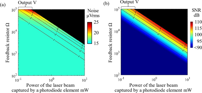
Estimated noise level and signal-to-noise ratio a Noise level b Signal-to-noise ratio

The theoretical equations described above reveal that the noise component of each element can be changed depending on the signal bandwidth. The change in each noise component as a function of signal bandwidth is calculated on the basis of the parameters summarized in Table 1. This summary is made under the condition that a silicon PD with a sensitivity of 0.2 A/W at a wavelength of 405 nm [28] captures a laser beam with a wavelength λ of 405 nm and a power of 2 mW. The resistance of the feedback resistor is set to 10 kΩ; therefore, the voltage output of the PD element becomes 4 V. The sampling frequency is set to twice the signal bandwidth. Figure 4 shows the results. The figure reveals that the contribution of the ADC is dominant, followed by the shot noise generated by the photocurrent due to incident light, current noise in the feedback resistor, and 1/f noise of the trans-impedance amplifier. The above calculations are conducted assuming the use of a commercial data acquisition (DAQ) system having ADCs with a 24-bit resolution (NI-9202, National Instruments [29]). Employing a DAQ system with a lower noise component than the aforementioned in a general experimental environment is difficult from a cost perspective. On the other hand, the contributions of the ADC and photocurrent IPD can be reduced by lowering the signal bandwidth. The total noise is calculated to be reduced to approximately 6.6 μVrms by lowering the cutoff frequency to 160 Hz.

Estimated noise components in the voltage signal of a photodiode element
It should be noted that attention should be focused on the quality of the electric power supply for the signal processing circuit. In the following experiments, an ultralow-noise DC–DC converter module with a noise level of approximately 30 μVrms is employed. Regarding the power supply rejection ratio (PSRR) of an ordinary op-amp (− 95 dB in the worst case [27]), the contribution of the electric power supply is calculated as 30 [μVrms] × 10−95/20 = 5.33 × 10⁻⁴ [μVrms] [30]. This value is almost negligibly small compared to other noise components in this application.
Moreover, the influence of the light intensity fluctuations induced by the instability of the laser source can be reduced through the arithmetic operation based on Eq. (2). However, the influence cannot be ignored if the PD output fluctuation due to light intensity fluctuations is extremely large compared to the contributions of other noise sources.
3 Estimation of the Feasible Resolution
3.1 Evaluation of the Sensitivity Distributions of PD Elements
Understanding the sensitivity profiles of PD elements employed in the angle sensor is necessary to estimate the sensitivity of angular displacement measurements. In this study, the sensitivity profiles of the elements in the dual-element PD, which was employed in the experiments described in the following section of this paper, were first evaluated by scanning a focused laser beam over the photosensitive surface. Figure 5 shows the experimental setup. A laser beam with a wavelength of 405 nm and a power of 2 mW was collimated into a beam with a diameter of 6 mm and focused onto the photosensitive area by a lens with a focal length of 40 mm. Preliminary measurements with a beam profiler confirmed that the spot diameter of the focused laser beam was approximately 5.6 μm, which was close to the diffraction limit. The parameters for the electronic circuit employed in the experiments are summarized in Table 2. Figure 6a shows the results. Notably, the output voltage is negative due to the characteristics of the trans-impedance amplifier. The results show that the voltage output of a PD element changed even when the adjacent PD element was irradiated by the focused laser beam. Figure 6b shows the sensitivity profile of the edge of each PD element calculated on the basis of the results shown in Fig. 6a. In the following numerical calculations, the resolution of angular displacement measurement is estimated on the basis of the sensitivity profiles shown in Fig. 6b.

Setup for the evaluation of the sensitivity distributions of adjacent photodiode (PD) elements

Sensitivity profiles of the adjacent photodiode (PD) elements a Voltage output level of the outputs of PDA and PDB b Sensitivity profiles of PDA and PDB
3.2 Estimating the Feasible Resolution by Numerical Calculations
The feasible resolution of angular displacement measurement is estimated by using the sensitivity profiles of the PD elements. From Eqs. (1) and (2), the following equation can be obtained:
where SM [arc-second−1] corresponds to the sensitivity of the angular displacement measurement. In an actual angle sensor, SM is obtained through a calibration process with an external angle sensor. Therefore, the angular displacement ΔθY can be obtained on the basis of the observed voltage outputs VA and VB of the two adjacent PD elements. SM has nonlinear characteristics considering ΔθY [12]; however, SM can be regarded as approximately linear in the region where ΔθY is small. According to the results of numerical calculations described below, under conditions of f = 100 mm and D = 10 mm or less, the range of at least ± 5 arc-seconds can be treated as a nearly linear region where the coefficient of determination R2 = 0.999 or more can be ensured during linear fitting.
It should be noted that, reducing the influence of fluctuations in the power of the measurement laser beam as well as the reflectance variations of the surface to be measured is possible by performing an arithmetic operation based on Eq. (15). The standard deviation σH of the normalized output of the angle sensor H can be calculated by the following equation:
where σVA and σVB are the standard deviations of the voltage outputs VA and VB of PDA and PDB, respectively, corresponding to the noise levels of the voltage outputs of PD elements in Vrms calculated in Sect. 2. Finally, the resolution of angular displacement measurement θres can be estimated on the basis of the following equation:
The feasible sensitivity and resolution of angular displacement measurement by an optical angle sensor with a dual-element PD are estimated by numerical calculations based on theoretical equations. Figure 7 shows a model for the numerical calculations. The model assumes that angular displacements in a step of 0.1 arc-second are given to a plane mirror reflector, and the measurement laser beam with the diameter D reflected from the mirror reflector is focused by a collimator objective with the focal length f on PDA and PDB having the sensitivity profiles shown in Fig. 6b. Parameters in Tables 1 and 2 are applied to the numerical calculations. Figure 8 shows an example of the calculation result of the change in the normalized output H considering the angular displacement given to the mirror reflector, from which the sensitivity SM of the angle sensor can be estimated. The resolution of the angle sensor is estimated on the basis of Eq. (17) by using the obtained SM. Figure 9a shows the calculated relationship among D, f, and SM. The diameter d of the focused laser beam at each combination of (D, f) is also represented by contour lines in the figure. D and d are defined as 1/e2 width. It should be noted that, SM is calculated on the basis of changes in H when the mirror reflector is subjected to an angular displacement of ± 5 arc-seconds. Figure 9b shows the variation of SM as a function of D at a focal length f of 10, 30, 50, and 100 mm extracted from the data shown in Fig. 9a. The figure reveals that the sensor sensitivity is estimated to increase as d decreases. Thus, the sensor sensitivity can be improved by reducing the focused laser spot diameter d by setting the measurement laser beam diameter D as large as possible when using a collimator objective with a certain focal length f. However, Fig. 9b shows that the contribution of increasing D to sensitivity improvement decreases with f. The results shown in Figs. 9a and b also indicate that high sensor sensitivity can be achieved with a long f even with the same focused laser spot diameter d. This phenomenon is due to the large travel distance Δx of the focused laser beam per angular displacement when f is long, as shown in Eq. (1). The range where the coefficient of determination R2 = 0.999 or higher can be ensured by linear fitting to the ΔθY – ΔH curve as a function of D at a focal length f of 20, 30, 50, and 100 mm extracted from the data (Fig. 9) is shown in Fig. 10. The figure reveals that the range of at least ± 5 arc-seconds can be treated as a nearly linear region under conditions of f = 100 mm and D = 10 mm or less.

Numerical calculation model of the sensor sensitivity based on theoretical equations

Estimated variation of normalized sensor output due to the angular displacement of a measurement target

Estimated sensor sensitivity a Contour plot of the estimated sensitivity at each (D, f) b Variation of the sensitivity at each f as a function of D

Variation of the linear region where the coefficient of determination R2 for linear fitting exceeds 0.999
Figure 11a shows the calculation result of the resolution θres based on the sensitivity presented in Fig. 9 and the standard deviations of the normalized outputs of PDA and PDB. Notably, the calculations are conducted under the condition that the cutoff frequency is set to 1 kHz.

Estimated sensor resolution a Contour plot of the estimated resolution at each (D, f) b Variation of the sensitivity at each f as a function of D
Figure 11b shows the variation of θres as a function of D at a focal length f of 10, 30, 50, and 100 mm extracted from the data presented in Fig. 10a. These results show that high-resolution angle measurement can be achieved by setting the focal length f as large as possible. In most cases, the resolution of an angle sensor using a segmented PD has been limited to 0.01 arc-second [12, 21, 31, 32] in previous studies. However, the results of theoretical calculations in this paper indicate that a resolution of better than 0.001 arc-second can be expected by reducing the noise in the sensor signal as well as designing the optical system appropriately.
4 Experiments
4.1 Development of the Experimental Setup
Based on the results of the numerical calculations, an experimental setup was designed and constructed on the basis of the numerical calculation results. Figure 12a shows a schematic of the setup. A pigtail laser diode (LD) with a wavelength of 405 nm and a power of 10 mW was employed as the laser source. A collimating lens with a focal length of 11 mm and an N.A. of 0.3 was used to collimate the laser beam from LD to 2 mm in diameter. A beam expander was also employed to adjust the diameter of the measurement laser beam. The linearly polarized (p-polarized) measurement laser beam was made to pass through a PBS and a QWP and was then projected onto a plane mirror reflector as circularly polarized light. A plate-type PBS was employed to avoid unwanted internal reflections. The measurement laser beam reflected by the plane mirror was made to pass through QWP again to become s-polarized light, which was then reflected by PBS. Finally, the measurement laser beam was captured by an autocollimation unit comprising a collimator objective and a PD.

Experimental setup for the evaluation of basic characteristics of the developed angle sensor a System configuration b A three-dimensional image and a photograph of the setup
In the autocollimation unit, the PD was placed on a two-axis manual stage, and the collimator objective was mounted on a single-axis stage traveling along the laser axis such that the photosensitive area would coincide with the focal plane of the collimator objective. A dual-element PD (S4204, Hamamatsu Photonics K.K.) with a gap of 20 μm was employed and mounted directly on a signal processing circuit board to minimize the wiring length from PD elements to the trans-impedance amplifiers for reducing the noise in the sensor signal. A guarding pattern is also placed around the wiring from the PD elements to the inverting input of the trans-impedance amplifier. The parameters of the other components used in the circuit were the same as those summarized in Table 2. The voltage signals of the two PD elements were then captured by the DAQ system with 24-bit ADCs (NI-9202, National Instruments). When evaluating the sensitivity of the angle sensor, the mirror reflector was mounted on a two-axis tilt holder, while another mirror reflector was placed on the back of the former mirror reflector to measure the given angular displacement with a commercial laser autocollimator with a resolution of 0.01 arc-second (LAC-S, Chuo Precision Industrial Co., Ltd.). Figure 12b shows a three-dimensional view and a photograph of the constructed optical angle sensor.
Notably, the optical head of the angle sensor can be designed efficiently by omitting the beam expander, which was employed in this paper to evaluate the effect of the measurement laser beam diameter D on the sensor sensitivity. In some applications, angular measurement is also performed by irradiating the measurement laser beam onto a rough surface compared to these reflective mirrors. In this case, the waviness frequencies and their amplitudes, Sa and Sq, of the reflector could affect the scattering of the reflected laser beam, resulting in degradations of sensor sensitivity and resolution. In this study, a flat mirror reflector with a specification (λ/10 at 633 nm) compatible with commercially available autocollimators was employed throughout all experiments.
4.2 Evaluation of the Sensor Resolution
First, the sensitivity of the constructed optical angle sensor was evaluated in experiments. The variation of the optical angle sensor output H was then observed when an angular displacement around the Y-axis in a step of approximately five arc-seconds was given to the mirror reflector mounted on a manual tilt stage. The cutoff frequency of the low-pass filter in the signal processing circuit was set to 1 kHz. At each angular position, the voltage signals of PD elements were sampled at a frequency of 2 kHz for 1 s. Figure 13a shows the result in the case of D = 2 mm and f = 50 mm. Meanwhile, Fig. 13b shows the sensor sensitivity calculated on the basis of the sensor output variation obtained for the range of angular displacement from − 5 arc-seconds to + 5 arc-seconds. High sensitivity was obtained for a large f; this result agrees with those obtained in the results of the numerical calculations. This finding is thought to be due to the large displacement of the focused laser beam on the photosensitive area of PD per angular displacement given to the flat mirror. Meanwhile, the experimental results showed that the increase in D resulted in the degradation of sensor sensitivity. These results are the exact opposite of those of the numerical analysis calculation shown in Fig. 9. One possible cause of this phenomenon is damage to the PD due to the focused laser beam, which is focused on a micrometric diameter. Figure 14 shows microscopic images of the PD surface after the experiments. Figure 14a is the image obtained when the photosensitive surface is highlighted, and Fig. 14b shows the one obtained when the resin cover on the PD element is emphasized. In this experiment, repetitive trials were performed while the diameter D of the measurement laser beam was expanded gradually. After adjusting the diameter, the sensitivity was evaluated after allowing time for the system to stabilize. Thus, the increase in D caused the reduction in the diameter of focused laser beam d on the PD, resulting in an increase in the power density of the laser beam that exceeded the allowable range of the resin cover of PD. In the series of experiments, no sensitivity degradation was observed even after repeated experiments with the laser beam irradiated at the same position on the PD under the conditions of P = 2 mW, D = 2 mm, and f ranging from 30 to 50 mm. However, under the conditions of D = 4 mm or higher and f ranging from 30 to 50 mm, a sensitivity degradation was observed after repeated experiments with the laser beam irradiated at the same position on the PD. These results indicate that the allowable power density of the PD used in this study was evaluated to be approximately 5 kW/cm2. This result suggests that the laser tolerance of the PD should be considered in the actual setup, and the focused spot on the PD cannot be designed to be extremely small. In this paper, considering the laser intensity tolerance of the employed PD, D was set to 2 mm in the following experiments.

Sensitivity of the developed angle sensor a Variation of the normalized output by the angular displacement given to the mirror reflector b Variation of the sensitivity with respect to the angular displacement given to the mirror reflector

Photodiode surface damaged by the focused laser beam a Focused on the photosensitive surface b Focused on the top cover of photodiode
The signal noise of the optical angle sensor was then evaluated. First, the signal noise was assessed without irradiating the laser beam onto PD. Figure 15a shows an example of the observed waveform of the voltage output of each PD element. The cutoff frequency of the low-pass filter in the signal processing circuit was then set to 1 kHz. Figure 15b shows the variation of signal noise considering the sampling frequency. At each sampling frequency, 10 repetitive trials for 1 s were performed, and the mean voltage level in Vrms is plotted in the figure. The maximum and minimum voltage levels in Vrms are also indicated in the figure. The contribution of the ADC during data acquisition was evaluated to be approximately 13 μVrms at a sampling frequency of 2 kHz. This value agrees with the estimated noise component.

Signal waveforms of the photodiode elements when the measurement laser beam was projected onto the mirror reflector mounted on a rigid holder a PDA b PDB c Normalized output
Second, the signal noise of the optical angle sensor was evaluated while irradiating the laser beam onto the PD. The mirror reflector was mounted on a fixed mirror mount, and the voltage signals of the PDA and PDB were captured simultaneously. The measurement laser beam reflected by the mirror reflector focused on the midpoint of PDA and PDB. Figure 16 shows typical waveforms of the voltage outputs of PD elements captured under the conditions of D = 2 mm and f = 40 mm. The normalized output H calculated on the basis of Eq. (2) is also plotted in the figure. The noise levels of the voltage signals of PDA and PDB were evaluated to be 224 and 153 μVrms, respectively, and the RMS value of the normalized output HRMS was evaluated to be 3.03 × 10⁻⁵ under a cutoff frequency of 1 kHz and a sampling frequency of 2 kHz. Considering the previously obtained sensitivity SM (0.0426 arc-second−1), the angular resolution was evaluated to be 7.12 × 10⁻⁴ arc-second. The resolution did not reach the value (3 × 10⁻⁴ arc-second) estimated to be achieved in the numerical calculations under the ideal condition. However, this value was found to be better than the result obtained in the previous study [22], where the bandwidth was limited to 12.5 Hz.

Signal noises of the photodiode (PD) elements without irradiating a focused laser beam a Voltage signals of PD elements b Variation of the signal noise as a function of the sampling frequency
Figure 17 shows the free vibration of the plane mirror reflector mounted on a manual kinematic mirror mount as measured by the developed optical angle sensor. The experimental result demonstrated that the developed optical angle sensor could detect the small angular displacement of the flat mirror reflector with an amplitude of 2 × 10⁻³ arc-second and a frequency of approximately 5 Hz.

Waveform of the normalized sensor output when the measurement laser beam was projected onto the mirror reflector mounted on a manual tilt stage
5 Summary
A feasible resolution of an optical angle sensor based on laser autocollimation with a multi-element PD has been investigated in numerical calculations and experiments. First, the contribution of each noise factor has been examined on the basis of theoretical equations. The results have revealed the dominant noise components of angle sensors that can employ a reflective mirror as a target to ensure a sufficient amount of light incident on the PD. These components are the signal acquisition noise in the ADC and the shot noise generated by the photocurrent due to the incident light on the PD. Afterward, the feasible sensor sensitivity was estimated on the basis of numerical calculations. This estimation considered the influences of the measurement laser beam diameter and the focal length of a collimator objective that focuses the laser beam onto PD, as well as the sensitivity profiles of the PD elements. The feasible resolution of the angle sensor with a dual-element PD has been estimated on the basis of the estimated noise components and sensor sensitivity. The results have revealed that a resolution better than 0.001 arc-second can be achieved even when the focal length of the collimator objective is set to less than 100 mm. An optical angle sensor has been developed on the basis of the above calculation results, and experiments have been performed. Attention has been provided to reducing the signal noise of the angle sensor by directly mounting a PD on a signal processing circuit board. Experimental results have confirmed that the signal noise of the angle sensor has successfully been suppressed to 13 μVrms with a bandwidth of 1 kHz. Moreover, the sensor sensitivity has been evaluated while changing the focal length of the collimator objective and the diameter of the measurement laser beam. The experimental results have clarified that the PD employed in this paper cannot accept a focused laser beam with a power density beyond 5 kW/cm2. These results have also demonstrated that sensor sensitivity can be improved by employing a collimator objective with a large focal length. Experimental results have demonstrated that, under the condition where P = 2 mW, f = 40 mm, and D = 2 mm, a resolution of 7.12 × 10⁻⁴ arc-second can be achieved by the developed optical angle sensor with a bandwidth of 1 kHz, which is substantially better than those achieved by the conventional optical angle sensor based on laser autocollimation.
It should be noted that this paper has focused on the study of the feasible resolution of angle measurement. The measurement range, measurement uncertainty, flatness, and surface roughness of the object to be measured, as well as other factors, have been disregarded. Meanwhile, these factors are important in considering the actual applications of optical angle sensors and will be considered in future work. The establishment of a method that can realize high resolution over a wide angular range is desired and will be addressed in future work.
Availability of Data and Materials
The authors declare that all data supporting the findings of this study are available on request from the corresponding author.
References
Gao W, Kim SW, Bosse H, Haitjema H, Chen YL, Lu XD, Knapp W, Weckenmann A, Estler WT, Kunzmann H (2015) Measurement technologies for precision positioning. CIRP Ann Manuf Technol 64:773–796. https://doi.org/10.1016/j.cirp.2015.05.009
Renishaw plc (2019) The accuracy of angle encoders. https://www.renishaw.com/en/the-accuracy-of-rotary-encoders--47130. Accessed 26 Apr 2023
Taylor H (2023) Autocollimators. https://www.taylor-hobson.com/products/alignment-level/autocollimators. Accessed 26 Apr 2023
Trioptics (2023) TriAngle - electronic autocollimator for precise optical angle measurement. https://trioptics.com/products/triangle-electronic-autocollimators/. Accessed 26 Apr 2023
MÖLLER-WEDEL OPTICAL GmbH electronic autocollimators. In: 2023. https://www.haag-streit.com/moeller-wedel-optical/products/electronic-autocollimators/. Accessed 26 Apr 2023
Auto collimator -CHUO PRECISION INDUSTRIAL CO., LTD. https://www.chuo.co.jp/english/contents/hp0198/list.php?CNo=198&ProCon=5874. Accessed 26 Apr 2023
Gao W, Arai Y, Shibuya A, Kiyono S, Park CH (2006) Measurement of multi-degree-of-freedom error motions of a precision linear air-bearing stage. Precis Eng 30:96–103. https://doi.org/10.1016/J.PRECISIONENG.2005.06.003
Quan L, Shimizu Y, Xiong X, Matsukuma H, Gao W (2021) A new method for evaluation of the pitch deviation of a linear scale grating by an optical angle sensor. Precis Eng 67:1–13. https://doi.org/10.1016/j.precisioneng.2020.09.008
Bitou Y, Kondo Y (2016) Scanning deflectometric profiler for measurement of transparent parallel plates. Appl Opt 55:9282. https://doi.org/10.1364/ao.55.009282
Zumbahlen H (2008) Linear circuit design handbook. Newnes, Elsevier
Klipec BE (1967) Reducing electrical noise in instrument circuits. IEEE Trans Indus General Appl. https://doi.org/10.1109/TIGA.1967.4180749
Gao W (2010) Precision nanometrology. Springer, London
Perpiñà X, Jordà X, Vellvehi M, Millán J, Mestres N (2005) Development of an analog processing circuit for IR-radiation power and noncontact position measurements. Rev Sci Instrum 76:49. https://doi.org/10.1063/1.1851472/926308
Wang C, Yu X, Gillmer SR, Ellis JD (2015) Robust high-dynamic-range optical roll sensing. Opt Lett 40:2497–2500. https://doi.org/10.1364/OL.40.002497
Kiyono S, Kamada O, Huang PS (1992) Angle measurement based on the internal-reflection effect: a new method. Appl Opt 31:6047–6055. https://doi.org/10.1364/AO.31.006047
Kasevich MA, Dickerson S, Chiow S-W, Johnson DMS, Hammer J, Kovachy T, Sugarbaker A, Hogan JM (2011) Precision angle sensor using an optical lever inside a Sagnac interferometer. Opt Lett 36:1698–1700. https://doi.org/10.1364/OL.36.001698
Pisani M, Astrua M (2006) Angle amplification for nanoradian measurements. Appl Opt 45:1725–1729. https://doi.org/10.1364/AO.45.001725
Pisani M, Astrua M, Raj SBT (2020) Sensor for the characterization of 2D angular actuators with picoradian resolution and nanoradian accuracy with microradian range. Sensors 20:7034. https://doi.org/10.3390/S20247034
Yuan J, Long X (2003) CCD-area-based autocollimator for precision small-angle measurement. Rev Sci Instrum 74:1362–1365. https://doi.org/10.1063/1.1539896
Ennos AE, Virdee MS (1982) High accuracy profile measurement of quasi-conical mirror surfaces by laser autocollimation. Precis Eng 4:5–8. https://doi.org/10.1016/0141-6359(82)90106-4
Saito Y, Gao W, Kiyono S (2007) A single lens micro-angle sensor. Int J Precis Eng Manuf 8:14–18
Shimizu Y, Tan SL, Murata D, Maruyama T, Ito S, Chen Y-L, Gao W (2016) Ultra-sensitive angle sensor based on laser autocollimation for measurement of stage tilt motions. Opt Express. https://doi.org/10.1364/OE.24.002788
Boyes W (2010) Instrumentation reference book. Elsevier, London
Hamamatsu photonics (2022) Si photodiodes. https://www.hamamatsu.com/content/dam/hamamatsu-photonics/sites/documents/99_SALES_LIBRARY/ssd/si_pd_kspd9001e.pdf. Accessed 26 Apr 2023
Seifert F (2009) Resistor current noise measurements. https://dcc.ligo.org/public/0002/T0900200/001/current_noise.pdf. Accessed 26 Apr 2023
Analog Devices (2022) ADA4522-1/ADA4522-2/ADA4522-4 data sheet
Analog Devices (2016) AD8661/AD8662/AD8664 data sheet
Hamamatsu photonics K. K. (2013) Si PIN photodiodes | S3096-02, S4204
NI NI-9202 Datasheet. In: 2023. https://www.ni.com/docs/ja-JP/bundle/ni-9202-specs/page/overview.html. Accessed 29 Apr 2023
Analog devices (2009) Op amp power supply rejection ratio (PSRR) and supply voltages. MT-043 Tutorial.
Gao W, Saito Y, Muto H, Arai Y, Shimizu Y (2011) A three-axis autocollimator for detection of angular error motions of a precision stage. CIRP Ann Manuf Technol 60:515–518. https://doi.org/10.1016/j.cirp.2011.03.052
Saito Y, Arai Y, Gao W (2010) Investigation of an optical sensor for small tilt angle detection of a precision linear stage. Meas Sci Technol 21:054006. https://doi.org/10.1088/0957-0233/21/5/054006
Acknowledgments
Yuki Shimizu would like to thank Professor Wei Gao (Tohoku University) for providing some test equipment.
Funding
This research is supported by JST, Fusion Oriented Research for Disruptive Science and Technology (FOREST), Japan (JPMJFR2027); Mitutoyo Association for Science and Technology (MAST), Japan; and the Japan Society for the Promotion of Sciences (JSPS), Japan (22H01370).
Author information
Authors and Affiliations
Contributions
Conceptualization was contributed by YS; methodology was constributed by YS and HL; formal analysis and investigation were contributed by YS and HL; writing—original draft preparation, was contributed by HL and YS; writing—review and editing, was contributed by YS; funding acquisition was contributed by YS; resources were contributed by YS; supervision was contributed by YS.
Corresponding author
Ethics declarations
Conflict of Interest
The authors declare that they have no conflicts of interest.
Rights and permissions
Open Access This article is licensed under a Creative Commons Attribution 4.0 International License, which permits use, sharing, adaptation, distribution and reproduction in any medium or format, as long as you give appropriate credit to the original author(s) and the source, provide a link to the Creative Commons licence, and indicate if changes were made. The images or other third party material in this article are included in the article's Creative Commons licence, unless indicated otherwise in a credit line to the material. If material is not included in the article's Creative Commons licence and your intended use is not permitted by statutory regulation or exceeds the permitted use, you will need to obtain permission directly from the copyright holder. To view a copy of this licence, visit http://creativecommons.org/licenses/by/4.0/.
About this article

Cite this article
Lim, H., Shimizu, Y. Feasible Resolution of Angular Displacement Measurement by an Optical Angle Sensor Based on Laser Autocollimation. Nanomanuf Metrol 6, 32 (2023). https://doi.org/10.1007/s41871-023-00211-8
Received:
Revised:
Accepted:
Published:
DOI: https://doi.org/10.1007/s41871-023-00211-8