Wakefield acceleration

Abstract

The fundamental idea of Laser Wakefield Acceleration (LWFA) is reviewed. An ultrafast intense laser pulse drives coherent wakefields of relativistic amplitude with the high phase velocity robustly supported by the plasma. The structures of wakes and sheaths in plasma are contrasted. While the large amplitude of wakefields involves collective resonant oscillations of the eigenmode of the entire plasma electrons, the wake phase velocity ~ c and ultrafastness of the laser pulse introduce the wake stability and rigidity. When the phase velocity gets smaller, wakefields turn into sheaths. When we deploy laser ion acceleration or high density LWFA in which the phase velocity of plasma excitation is low, we encounter the sheath dynamics. A large number of world-wide experiments show a rapid progress of this concept realization toward both the high energy accelerator prospect and broad applications. The strong interest in this has driven novel laser technologies, including the Chirped Pulse Amplification, the Thin Film Compression (TFC), the Coherent Amplification Network, and the Relativistic Compression (RC). These in turn have created a conglomerate of novel science and technology with LWFA to form a new genre of high field science with many parameters of merit in this field increasing exponentially lately. Applications such as ion acceleration, X-ray free electron laser, electron and ion cancer therapy are discussed. A new avenue of LWFA using nanomaterials is also emerging, adopting X-ray laser using the above TFC and RC. Meanwhile, we find evidence that the Mother Nature spontaneously created wakefields that accelerate electrons and ions to very high energies.

1 Introduction

1.1 The basic philosophy

Conventional accelerators are by and large based on the single particle interaction of charged particles with the externally imposed accelerating fields (Chao et al. 2014). The dynamics is determined foremost by each charge particle interacting with the external fields and this is the single particle dynamics. Veksler suggested the idea of collective field acceleration in plasma (Veksler 1956), which triggered research in collective accelerators (Rostoker and Reiser 1979). Collective accelerators based on the collective interaction involved a large number (N) of particles, which give rise to fields that are collectively composed by these particles and those particles themselves interact with each other. Thus, collective fields (as opposed to the single particle interaction) are nonlinear.

We summarize the cardinal differences between the individual and collective forces. See Table 1. Here we contrast the nature of the individual force and acceleration based on this (and thus linear force and the conventional accelerators) with that of the collective force and acceleration based on the collective force. In this review we concentrate on the latter only. The single particle interaction with the externally imposed voltage on the metallic boundary suffers from the surface materials breakdown by sparks and arching. Metallic electrons may be subject to hop out of the metallic chemical potential into a free (with breakdown) state typically the surface field on the order of MeV/cm. But this happens more typically even under much lower field limit. This is because typical materials contain impurities, whose f-center can initiate sparks under a couple of orders of magnitude lower fields. There is an additional inconvenience due to the metallic surface, which causes the waveguide modes to have the phase velocity greater than the speed of light. This necessitates us to design the slow-wave structure by periodically imposing protruding structures into the waveguide to slow down the phase velocity. This unfortunately even help the breakdown from such protruding portions, making the breakdown more susceptible. Because of the accelerating fields are only in the parallel direction, which further projects only partial field strength available for the purpose of the acceleration in the conventional accelerating structure. In the right columns in Table 1, on the other hand, under the collective force in plasma, since plasma is already broken down, it won’t break down further. Thus, it is not limited by the break down of the surface metal. The typical fields that are realized is the so-called Tajima–Dawson field. Or they could be often even larger than this value if the relativistic effects are included. We will see this in detail later. The phase velocity of the wakefields is shown to be close to but slightly smaller than the speed of light c. The other distinction of the linear force vs. collective force is that the former needs to avoid large disturbances (“bang”), while the latter tolerates (or even “cherishes”) strong “banging” disturbances. We discuss why this distinction arises below.

Table 1 Individual vs. collective acceleration

Even though collective fields could be huge, as they involve N particles, if they are chaotic or random, their effects may be compromised by cancellation and randomization. To address this issue, we introduce coherence. In the year of 1956 before the invention of laser (1960) such coherence may have been achieved by the beam of particles (Veksler 1956). In fact the many of the experimental endeavors (Rostoker and Reiser 1979) electron beams have been employed. The injection of electron beams into plasma and create accelerating structure in these experiments have been examined by us (Tajima and Mako 1978). In these works, the electron beam injection often involved the sheath formation, which could give rise to instability, as the sheath structure is often stuck with the system’s boundary condition.

In the 1979 work, Tajima and Dawson noticed and introduced a high-speed structure (i.e., the phase velocity of the accelerating structure): the principle of high phase velocity. This high phase velocity structure they seek was the wakefield. The wakefield with high phase velocity, unlike the sheath created under the structural constraint, remains robust and stable. When one of us (TT) was watching a duck causing a wake behind it on the pond close to his university (when he was a student in Tokyo), he would see that the duck causes a well-sustained coherent wave structure lasting for a long time behind the duck (Fig. 1). This may be also explained by the principle of the hide-and-seek game (“Onigokko” game in Japanese) principle: the water wave (or in our case plasma wave) may not be easily destroyed when it has a high phase velocity, as electrons (or the seeker) notice the hider (wave), the hider (wave) is already gone when the seeker (electrons) just arrive the hider’s spot. In the following we dwell on more discussions on this high phase velocity principle.

Fig. 1

High phase velocity wakefield showing sustained and coherent structure by a duck or a motorboat. Immediately ahead of the duck (or the motor boat) we see the wave of water up (a bow wave), which emanates a triangular shaped bow (similar to a Mach cone). Behind the duck (or the motorboat) immediate water depression wave followed by oscillatory compensations of water high and low in a wavy pattern whose wavefront is perpendicular to the duck (or motorboat) progression direction. This wave is called wake (or stern wake) of the duck (or motorboat) motion. The duck (or motorboat) speed ((since its movement represent the energy flow of the object, we may call it the group velocity of the driving object. The propagation velocity (the phase velocity) of the pattern of the waves in the direction of the object (the duck or the boat) is equal to the group velocity of the object. We observe, however, that often the wave oscillations such as water level up and down are left out from the object and thus the group velocity of these waves are much less (sometimes 0) than the group velocity of the driver. On the upper left we show the wakes behind a motor boat. The tsunami wave off shore has a high phase velocity and propagates without much energy transfer to ships on the ocean water. One the other hand, when the tsunami approaches the shore, its phase velocity slows down so that its amplitude goes up and begins to trap the particles (such as ships) floating on the water or even on the floor of the shore (see Sect. 7). And these heightened water wave amplitude of tsunami on shore begins to go beyond the water wave-breaking limit, showing white foamy breaking water (upper right). A duck makes his wake (lower left). Geese ride on the bow wake behind the lead goose to save their energy (lower right)

In Table 2 we compare the low phase velocity interaction with the high phase velocity interaction and show our Paradigm of High Phase Velocity. Here the plasma remains robust and stable, while it accepts (and in fact “loves”) large amount of banging such as injection of intense laser or relativistic bunched beams. We learn that plasma suffers from a large variety of instabilities (Mikhaĭlovskiĭ 1974) in the conventional situation, where the phase velocity of the waves $v_{{{\text{ph}}}}$ is on the order of the thermal velocity $v_{{{\text{th}}}}$. On the other hand, our paradigm dictates that the excited wave (wakefields) has the phase velocity far greater than the thermal velocity of the bulk plasma. One of important consequences of this principle is the structure formation. When the phase velocity of the “banging” is large, behind the “banging” we observe a structure called wakefields. These are moving with a large phase velocity (such as near c) that is sustained by electrons while often such a structure has a low (or zero) group velocity (and ions do not move). On the other hand, when the phase velocity of such a “banging” is low (or near zero), the electrons that are “banged” begin to move but cannot propagate with the large phase velocity characteristic of the high phase velocity counterpart. Therefore, the electrons cannot continuously propagate and instead snap back due to the electrostatic charged restoring force. This is the sheath formation as opposed to the wake formation. See the bottom row of Table 2. Because of this low phase velocity sometimes ions can respond to this. Under certain boundary conditions in turn the entire plasma may begin to move (i.e., ion acceleration is accompanied). This latter situation may in fact correspond to Prof. Rostoker’s early vision (discussed again in Sect. 4). And the sheath acceleration called TNSA (2000) and other later laser ion accelerator schemes). We also see the similar situation in the high density regime of laser wakefield acceleration (Nicks et al. 2019) and in Sects. 3 and 7. However, we are primarily focusing on the high phase velocity cases in the present paper.

Table 2 High phase velocity paradigm

Some of these wake dynamics (both bow and stern) are shown in Fig. 1. The robust wakefields are shown in contrast to the case when the phase velocity of the wave gets small (in the case of tsunami near the shore). We will see some of the utilization of the wakefield’s phase velocity in the plasma density change strategies in later chapters. In Fig. 2, we show the moment of the large amplitude water wave break (left) and after that (with white foamy crest) (right). These are nonrelativistic water waves. In wakefields driven by laser or relativistic charged particles the relativistic dynamics of electrons helps further robustness of the wakefields, as shown in Fig. 3 (left). This additional stabilizing robustness was referred to the relativistic coherence (Tajima 2010) as discussed in Table 3. We also note that wakefields may be driven even in the quark-gluon plasma inside of heavy nuclei driven by energetic hadron beam [or even in superstring theory (Maldacena 1999)]. Nuclear quark-gluon wakefields are shown in Fig. 3 (right). From now on we will focus on plasma wakefields.

Fig. 2

Shore wave right before and about the breaking (left). The classical water break of a large amplitude water wave captured by Hokusai. It also shows the foamy wave breaking in its nonrelativistic wave break (right)

Fig. 3

Laser wakefield (1D PIC simulation), showing a robust non-wavebreaking peaked electron density (left). QCD wakefield (Chesler and Yaffe 2008) (right)

Table 3 Relativistic coherence

1.2 Nature of coherence in the strong “bang” (laser pulse) in wakefields

To embody these organizational principles, Tajima and Dawson (1979) proposed the employment of an ultrashort and intense laser pulse to excite a wakefield in such a way that the laser pulse length $l_{0}$ is resonant to the wavelength of the eigenmode of the plasma, i.e., half of the plasma wavelength $l_{{\text{p}}} = 2\pi c/\omega_{{{\text{pe}}}}$. This choice of resonant wavelength is to efficaciously excite coherent eigenmode of the plasma without causing other disturbances in it, satisfying the first guiding principle above. The laser in the underdense plasma speeds at the group velocity close to the speed of light, which of course is much higher than the thermal speed of electrons, realizing the above second condition. Such a short pulse length to make the plasma wavelength resonance is in the fs regime, thereby not disturbing ions. This embodies the fourth principle above. In most recommended cases, we select the frequency of the laser much higher than the plasma frequency, which leads to set the Lorentz factor $\gamma_{{\text{p}}}$ of the phase velocity of the wakefield much greater than unity. This introduces relativistic coherence, the guiding direction mentioned as third above. The recommended intensity of the laser pulse is such that the ponderomotive potential (the photon pressure force potential) of the laser in the plasma amounts to $\Phi = mc^{2} \sqrt {1 + a_{0}^{2} }$ so that the excited plasma wave motion acquires the electron momentum of $mca_{0}$. Here the normalized vector potential of the laser is $a_{0} = eE_{0} /m\omega_{0} c$ and $E_{0}$, $\omega_{0}$ are the electric field and frequency of the laser. The ponderomotive force arises from the non-linear Lorentz force $v \times B/c$, which causes the polarization of electrons in the plasma in the longitudinal direction, even though the electric field of the laser is in the transverse direction. This yields the electrostatic field $E_{{\text{p}}} = m\omega_{{\text{p}}} ca_{0} /e$ in the longitudinal direction in the same magnitude. This is the rectification of the transverse field of laser into the longitudinal wakefield. This is the origin of the excited wakefield. When $a_{0}$ of the laser is greater than unity, such a laser is called relativistic (intensity). At the verge of relativistic strength, i.e., $a_{0} = 1$, the wakefield amplitude assumes the value of $E_{{\text{p}}} \left( {a_{0} = 1} \right) = m\omega_{{\text{p}}} c/e$. This is the wave breaking field in the non-relativistic case. The wave tends to break if the wave amplitude is high so that the high amplitude portion of the wave typically propagates faster than the lower portions and takes over those. The relativistic phase of intense laser also makes the amplitude of the wakefield $E_{{\text{p}}}$ relativistically intense, i.e., $a_{{\text{p}}} = eE_{{\text{p}}} /m\omega_{{\text{p}}} c$ greater than unity. Note here to distinguish the phase velocity of wakefield being relativistic ($\gamma_{{\text{p}}} \gg 1$) and the laser amplitude being relativistic $a_{0} \gg 1$. However, it is of interest to recognize that the latter $a_{0} \gg 1$ provides the relativistic coherence to the wakefield and the realization of relativistically coherent wakefield possible $a_{{\text{p}}} \gg 1$ (Tajima 2010). In addition to the coherence garnered by the excitation of the collective eigen mode of plasma [the typically the Langmuire plasma mode (electrostatic in its origin, but can acquire electromagnetic characters from the 2–3 dimensional effects and boundary conditions)] in this ultra-relativistic regime we attain the relativistic coherence, as the relativity dictates that particles move at near speed of light when they become highly relativistic. Thus, in this regime all particles move synchronously at the same speed thus attaining additional coherence and robustness arising from this. Thus, wakefield tends to become more robust, when they are driven with more “bang” (more intense drivers). As we will discuss in astrophysical implications later, this is one of the important considerations why wakefields are naturally manifested in cosmic phenomena, where naively it appears that nature does not have control for coherence, as opposed to human-imposed experiments. The fact of matter, it appears often, is that this predominance of the biggest “bang” in the naturally occurring phenomena can dictates the most significant development in the dynamics and thus somewhat surprisingly on the surface (but not so in retrospect) strong coherent dynamics of wakefields can arise naturally in nature. See Table 3. In the optics since the invention of laser, it brought in coherence, as laser is the coherent photons. The quantum coherence has been well-known using laser properties. However, we introduce relativistic coherence as shown in Table 3.

Once we introduce the method and mechanism behind relativistically coherent and robust wakefield as above by the short pulsed electromagnetic (EM) waves [laser wakefield accelerator (LWFA)], it is not difficult to also introduce the wakefield driven by a bunch of relativistic charged particle (such as electron bunch (Chen et al. 1985) in fact the original thought by Rostoker et al. (1979) was generically in this category and ion bunch (Caldwell et al. 2009). In the latter the charged particles’ electric fields point in the radial direction, while the magnetic fields introduced by the beam current are in the azimuthal direction, making the ponderomotive force essentially identical to the pulsed EM (or laser) waves. We may call all these methods as wakefield acceleration as a whole.

We summarize characteristics of the coherence emerging from the wakefield physics. The laser (or energetic beam injection) injected into the underdense plasma has a high group velocity (Tajima and Dawson 1979). Because of this, the phase velocity of the wake excited by the laser pulse [which is equal to the group velocity of the laser (or the beam)] is also high (close to the speed of light). Thus the wakefield phase velocity is far removed from the actions of the bulk thermal activities (v_ph >> v_th). This maintains the wakefields be largely insulated from the plasma bulk instabilities. This is why wakefields, once excited, remain high amplitude robust waves that are well maintained. This is akin to the wakes excited by a duck swimming on the surface of a lake, whose wakes are well preserved in the trail of the duck (or equivalent motorboat wakes). See Figs. 1 and 2. Also note that the excited wake has bow kinds of wakes. In the duck or motorboat wakes as well as the laser wakefields, we observe the bow wake that is excited ahead of the wake exciter (the duck, motorboat, or the laser pulse (or the bunched charged beams) and the stern wake behind of it. See Fig. 2. The bow wake plays the role of inducing the stern wake. In certain cases such as the astrophysical ultra-relativistic wakes, the frontal bow wakes are predominant (see Sect. 6). In other applications we discuss, such as ion acceleration, we wish to deliberately excite the phase velocity of the subsequent waves at small phase velocity so that it can capture slow moving ions. This strategy will be discussed later in Sect. 4.

Some of the consequences of the collective excitation of modes that have principle of high phase velocity are summarized in Table 2. In the typical plasma, instabilities happen when the phase velocity $v_{{{\text{ph}}}}$ is close to the thermal velocity $v_{{{\text{th}}}}$ in such instabilities as the drift wave instability:

$$\begin{array}{*{20}c} {v_{{{\text{ph}}}} \sim v_{{{\text{th}}}} ,} \\ \end{array}$$

(1)

When this is the case, if and when a wave is excited by some instability at the phase velocity $v_{{{\text{ph}}}}$, the wave can grow till it can trap electrons according to O’Neil (1965) at the trapping with is given by

$$\begin{array}{*{20}c} {v_{{{\text{tr}}}} = \sqrt {qE/mk} ,} \\ \end{array}$$

(2)

where E is the electrostatic wave amplitude, k is the wavenumber of its wave, and q and m are the charge and mass of that particle that is to be trapped. In the condition (1) the wave phase velocity sits in the middle of the plasma particle distribution in its phase space so that even before the trapping width becomes substantially large, particles are trapped and begin to modify the distribution function significantly. This is the classical way that most plasma-wave particle interaction under O’Neil’s mechanism. In contrast to this, when the wakefields are excited as

$$\begin{array}{*{20}c} {v_{{{\text{ph}}}} \gg v_{{{\text{th}}}} ,} \\ \end{array}$$

(3)

where $v_{{{\text{ph}}}}$ in laser wakefields is often close to c. Thus in the paradigm of the large phase velocity, the wave (such as wakefields) cannot trap electrons, as they are far removed from the region of where the phase velocity sits in the velocity space. Thus, the wakfields are not modifying the bulk plasma (a similar situation to the tsunami wave off shore is not wrecking the ship on the off-shore sea). This is why the bulk plasma does not suffer instability by the presence of wakefields. In fact, only when the trapping width of the wakefields becomes so large to satisfy the condition, the wakefields can begin to trap the bulk electrons:

$$\begin{array}{*{20}c} {v_{{{\text{tr}}}} \sim v_{{{\text{ph}} }} \left( { \gg v_{{{\text{th}}}} } \right)} \\ \end{array}$$

(4)

and could begin to stop growing its amplitude. Since $v_{{{\text{ph}}}}$ ~ c and k = $\omega_{{\text{p}}} /c$, using Eqs. (2) and (4), we obtain

$$\begin{array}{*{20}c} {E{ } = E_{{{\text{TD}}}} = \frac{{m\omega_{{\text{p}}} c}}{e}.} \\ \end{array}$$

(5)

This value on the right side of Eq. (5) is the so-called Tajima–Dawson field. This is also the same as the non-relativistic wave breaking field (Berger and Newcomb 1958).

To drive such strong wave (wakefields), a superstrong laser pulse (or relativistic charged beam pulse) is desired to be imposed (laser wakfields or beam-driven wakefields). Because of the above paradigm of the high phase velocity, such superstrong fields are tolerated in plasma (unlike in the left column situations in a “typical” plasma) in Table 2. When we call a superstrong laser pulse as relativistic laser (or relativistically intense laser), it means that electrons are driven to relativistic energies (and thus reach near speed of light) by the oscillating laser electric fields (in its transverse direction) within one single laser oscillation. This means that the normalized vector potential a₀ = eE₀/mω₀c exceeds unity, where E₀ and ω₀ are laser electric field and frequency:

$$\begin{array}{*{20}c} {a_{0} = eE_{0} /m\omega_{0} c > 1.} \\ \end{array}$$

(6)

To excite a large amplitude of wakefield electric fields (longitudinal field and also can be some transverse fields in more than 1D), we wish not only to employ the above superstrong fields’ brute force, but also resort to the plasma’s ability to resonantly excite its eigen mode(s). The most important eigenmode in plasma is its Langmuir plasma oscillations (plasma wave). This is similar for a child to excite the swing to a large amplitude by sway it by its periodic eigen frequency, or a violinist stirs harmonic sound oscillations of its string vibration. To excite this collective mode of plasma, we set the laser pulse length l_l be a half of the eigen wavelength of the plasma wave (Tajima and Dawson 1979), that is

$$\begin{array}{*{20}c} {l_{{\text{l}}} = \pi c/\omega_{{\text{p}}} .} \\ \end{array}$$

(7)

There are other ways to also resonantly excite plasma eigenmodes, such as the beatwave, self-modulation instability of plasma (Tajima and Dawson 1979; Tajima 1985; Fisher and Tajima 1993; 1996).

The energy gain of electrons that are trapped by (or injected into, or surfing on) the wakefields may be calculated using the height of the ponderomotive potential Φ₀ of the laser:

$$\begin{array}{*{20}c} {\Phi_{0} = mc^{2} \left( {\sqrt {\left( {1 + a_{0}^{2} } \right)} - 1} \right).} \\ \end{array}$$

(8)

The amplification of the electron energy gain over the ponderomotive potential energy Φ₀ is by the Lorentz factor enhancement 2γ² (Tajima and Dawson 1979), which is obtained using the expression of the phase velocity $v_{{{\text{ph}}}}$ of the plasma wave of wakefields being $c\sqrt {\left( {1 - \omega_{{\text{p}}}^{2} /\omega_{0}^{2} } \right)}$:

$$\begin{array}{*{20}c} {2\gamma^{2} = 2\omega_{0}^{2} /\omega_{{\text{p}}}^{2} .} \\ \end{array}$$

(9)

This factor (9) arises due to the fact that the wave of wakefields are propagating with high phase velocity (with ions being stationary). As we will discuss in more detail in ion acceleration Sect. 4, in the case of sheath formation with low phase velocity (and also the case of wakefields in high density near the critical density, also to be discussed later) there is no energy enhancement due to this Lorentz factor enhancement. Instead in the case of Coherent Acceleration of Ions by Laser (CAIL)/Radiation Pressure Acceleration (RPA) acceleration there is the energy enhancement factor (2α + 1) over the ponderomotive potential Φ₀ (α: coherence parameter) (Mako and Tajima 1984), a different mechanism. See Table 2 the last row (left).

In addition to the conventional (laboratory) acceleration, also nearly all known astrophysical acceleration mechanisms [such as the Fermi acceleration (Fermi 1954)] are single particle acceleration and thus linear in its each stage. However, the Fermi acceleration in astrophysics assumes multiple scatterings of each ion over many encounters of magnetic clouds. In later sections we see that wakefield acceleration also takes place in astrophysical settings. Thus, Nature has employed also its own collective plasma force to drive wakefields and acceleration. Of course, the Mother Nature is tremendous and its acceleration is far beyond what we could marshal on the surface of the Earth.

In Table 3, we characterize the nature of relativistic coherence that emerges in our relativistic dynamics of the wakefield excitation. There is the well-known coherence phenomenon called the quantum coherence (Cohen-Tannoudji and Robilliard 2001). The quantum coherence emerges when the matter is ultracold and the atomic wave functions tend to show broader de Broglie wavelength in low temperatures. When the de Broglie length gets greater than the mean distance of atoms, wavefunctions of atoms or particles of atoms tend to show quantum overlap and thus coherence. Then such phenomena as superfluidity and superconductivity manifest. In the total opposite scale of energy is the relativistic coherence. When the particles’ energy become ultra-relativistic, their speeds all become near the speed of light ~ c and thus they tend to move together and acquire coherence. The formation of a thin electron sheet by the wakefields is a good example of this. Because of this relativistic coherence, the wakefields tend to be more coherent, robust, and regulated, as shown in Fig. 3 (left). It is also noted that because of the relativistic coherence the electron density, for example, tends to be more peaked than in the nonrelativistic cases, again seen clearly in Fig. 3 (left). If such relativistic effects are exercised in higher dimensions (such as in 2D or 3D), the incurred fields may be also enhanced because of such concentration. Another relativistic effect is worth mentioning. As we have seen above, the coherent dynamics in collective forces allows some special bonus in the ponderomotice force. The ponderomotive force arises by the Lorentz force (q/c) v × B. When the force is collective and coherent, the ponderomotive force is proportional to the time-average of the Lorentz force, $\left\langle {{\varvec{v}} \times {\varvec{B}}} \right\rangle$, which may be expressed proportional to the laser electric field squared averaged, $\left\langle {E^{2} } \right\rangle$, which is proportional to $a_{0}^{2}$. On the other hand, when the parameter a₀ becomes on the order of or greater than unity, i.e., relativistically intense, the electron dynamical velocity no longer is proportional to E ( or a₀), thus the ponderomotive force is proportional merely to a₀. We can see this in the expression of the ponderomotive potential $\Phi = mc^{2} \sqrt {1 + a_{0}^{2} }$. Even though in the relativistic regime (a₀ > 1) the ponderomotive potential does not increase as rapidly as in the nonrelativistic regime (a₀ < 1); however, we garner the relativistic coherence instead, whose benefits we have just discussed above.

2 Laser compression

One of the basic requirements for LWFA excitation (Tajima and Dawson 1979) mentioned in Sect. 1 is to have an ultrafast intense laser pulse compression (in the fs regime) to resonate with the collective eigenmode of plasma oscillations. The technique of Chirped Pulse Amplification (CPA) (Strickland and Mourou 1985) was invented timely (1985) to meet this requirement (1979). A major review on this demand and realization of CPA is found in Ref. (Mourou et al. 2006). Thus, we will not repeat this here. The CPA had spurred the experimental realization of LWFA in a major way. By so doing it further spurred along with LWFA the advent of high field science (Mourou et al. 2006; Tajima et al. 2000). The LWFA demands on the collider specs have further stimulated the intense laser technology in an entirely new direction and horizon as the invention of CAN (Coherent Amplification Network) fiber laser system (Mourou et al. 2013). This was to answer the call for high repetition rated, high efficiency intense laser needed for the high luminosity collider beam drivers (Xie et al. 1997; Leemans et al. 2011). In recent years there arose demands for high-energy LWFA demands low density of the accelerating plasma (or high frequency of laser drive). The lower the density is, the higher the laser energy required becomes. The initiative of compressing high energy lasers of nanoseconds into those in fs has also inspired methods for compression of high energy laser on one hand, while further compression desires (beyond CPA) of fs lasers into the regime of single-cycled laser (in a few fs) have arisen. The thin film compression (TFC) technique (Mourou et al. 2014) was born from this demand. In this section we will delineate this development in detail. It is remarkable to note that this single-cycled optical laser compression opened a way to create a single-cycled X-ray laser possibility, which would be never imagined as possible so readily till the arrival of TFC. This is because the earlier innovation of the relativistic mirror compression of optical laser pulse works best in converting a single-cycled regime of optical laser into single-cycled X-ray laser pulses (Naumova and Nees 2004; Naumova and Sokolov 2004). This development further opened a path toward the X-ray LWFA possibility (Tajima 2014).We briefly review on this in Sect. 8. This is an alternative way to access LWFA scaling by increasing the critical density instead of decreasing the plasma density. Such developments revolutionize both ultraintense lasers (into EW lasers) and ultrafast pulse lasers (into zeptoseconds), as predicted by the Pulse Duration-Intensity Conjecture (Mourou and Tajima 2011). Such laser pulses are so unique that we still need a lot to learn in the future on their implications.

There is a tendency to think that ultrashort pulse is the appanage of small-scale laser. In the pulse duration-peak power conjecture (Mourou and Tajima 2011) the opposite was demonstrated. Pulse duration and peak power are entangled. To shorten a pulse, it is necessary first to increase its peak power. In this article we show an example that illustrates this prediction, making possible the entry of laser into the zeptosecond and exawatt domain.

Since the beginning of the 1980’s optical pulse compression (Grischkowsky and Balant 1982) has become one of the standard ways to produce femtosecond pulse in the few cycle regime. The technique relies on a single mode fiber and is based on the interplay between the spectrum broadening produced by self phase modulation and the Group Velocity Dispersion necessary to stretch the pulse. The combination of both effects contributes to create a linearly frequency-chirped pulse that can be compressed using dispersive elements like grating pairs, prism pairs or chirped mirrors. In their pioneering experiment, Grischkowsky et al. (1982) used a single mode optical fiber and were able to compress a picosecond pulse with nJ energy to the femtosecond level. This work triggered an enormous interest that culminated with the generation of a pulse as short as 6 fs corresponding to 3 optical cycles at 620 nm by C.V Shank’s group (Knox and Fork 1985) see Fig. 4. In their first experiment the pulse was only 20 nJ, clamped at this level by the optical damage due to the core small size. To go higher in energy Svelto and his group (Nisoli et al. 1996) introduced a compression technique based on fused silica hollow-core capillary, filled with noble gases and showed that they could efficiently compress their pulses to the 100 μJ level. Refining this technique Nisoli and DeSilvestri (1997) could compress a 20 fs into 5 fs or 2 cycles of light at 800 nm, where the energy was typically sub mJ. In both cases, like with single mode fiber, the compression effect was still driven by the interplay between self-phase modulation and group velocity dispersion.

Fig. 4

Evolution of few optical cycle pulses over the years

To go higher in energy, bulk compression was attempted by Corkum and Rolland (1988). See Fig. 4. In their embodiment the pulse is free-propagating and not guided anymore. The pulse was relatively long around 50 fs with an input energy of 500 μJ leading to an output pulse of 100 μJ in 20 fs. This scheme is impaired by the beam bell shape intensity distribution. It leads to a non-uniform broadening compounded with small scale self focusing making the pulse impossible to compress except for the top part of the beam that can be considered as constant limiting the efficiency and attractiveness of this technique.

2.1 Thin film compression (TFC)

Here we are describing a novel scheme capable to compress 25 fs large energy pulses as high as 1 kJ to the 1–2 fs level. We call this technique Thin Film Compressor or TFC. See Fig. 5. The incoming already short laser pulse (such as 25 fs) goes through a thin film of dielectric, which phase modulate the laser pulse in broaden its spectrum. Once this optical nonlinearity makes the spectrum broadening, we can make the pulse compressed further by a pair of chirped mirror to further compress the laser pulse, say, by a factor of two. If one tried this process three rimes, one could compress the pulse eventually by an order of magnitude. As shown in simulation this technique is very efficient > 50% and preserves the beam quality (Mourou et al. 2014).

Fig. 5

Embodiment of a double Thin Film Compressor TFC Thin film “plastic” of 500 μm thickness as uniform as possible is set in the near field of PW producing a flat-top beam with the B-integral value (B) of about 3–7. The beam propagates through a telescope composed of 2 parabolae, used to adjust finely the B and reduce the laser beam hot spots. Before compression the beam is corrected for the residual wavefront non-uniformity of the beam and the thin film thickness variations. The pulse is compressed using chirped mirrors to 6.4 fs. The measurement is performed using a single shot auto-correlator. The same step is repeated in a second compressor with a film of 100 μm producing an output of 2 fs, 20 J (after Mourou et al. 2014)

Unlike in the previous bulk compression technique performed with large-scale laser exhibiting bell shape distribution, the technique relies on the top hat nature of large-scale femtosecond lasers when they are well constructed. Figure 6 shows the output of a PW laser generating 27 J in 27 fs called CETAL in the National Institute of Laser, Plasma and Radiophysics (NILPR) in Bucharest (see Ref. Mironov et al. 2017); its recent application is mentioned in Ref. Zhou and Yan (2016). Similar flat top energy distributions are exhibited by the BELLA system at Lawrence Berkeley Laboratory. The next generation of high power laser will deliver 10PW like ELI-NP in Romania or Apollon in France, with a similar top hat beam. Simulation shows that the pulse being already very short, i.e., 27 fs will require a very thin optical element of a fraction of a mm thick for a beam of 16 cm diameter. This element will be extremely difficult to manufacture, extremely fragile to manipulate and very expensive, making the idea of pulse compression of high energy pulse unpractical. Our solution is to use a thin “plastic” film of ~ 500 μm with a diameter of 20 cm. The element, that we call plastic for simplicity could be amorphous polymer thermoplastic, like the PVdC (polyvinylidene chloride), the additive PVC (polyvinyl chloride), the triacetate of cellulose, the polyester, or other elements as long as they are transparent to the wavelength under study, robust, flexible and exhibit a uniform thickness, ideally within a fraction of a wavelength. It is paramount to have a thickness as uniform as possible across the beam, but does not have to be flat. As opposed to a thin (fraction of a mm) quartz, silicate over a dimension of 20 cm, it is abundant, inexpensive and sturdier. It should be susceptible to withstand the laser shot without breaking. In case where the film breaks, it can be replaced, cheaply, easily for the following shot. In the preferred embodiment shown in Fig. 5, the laser beam is focused by an off axis parabola with a f# about 10. The focused beam plays two roles. (a) It can be used to adjust the beam intensity by sliding the film up and down (over a small travel though) to optimize intensity and (b) to provide a means to eliminate the high spatial frequencies produced by the beam nonuniformities due to the small scale focusing. A pinhole of suitable dimension is located at the focus. After the focal point the beam is re-imaged to infinity by a second parabola. The pulse can be measured at this point using a standard single shot autocorrelator technique. Simulations, in the next chapter demonstrate the possibility to compress a 27 J, 27 fs into 6 fs in a first stage and 2 fs in a second stage, where the plastic thickness is 100 μm. The beam remains of good quality after this double compression, as shown in Fig. 6.

Fig. 6

This figure shows the intensity across the beam profile: a at the laser output, b after the first stage (no spatial filter, c after the second stage (no spatial filter) (after Mourou et al. 2014)

Because there is no real loss in the system we expect an overall compressor efficiency in the range > 50%. As a consequence, the peak power is increased close to 10 times. Note that ideally, after each “thin film” a wave front corrector is installed to take into account a possible non-uniformity of the film thickness that could not affect the B but would be harmful to the wave front. This simple technique provides a spectacular reduction in pulse duration of more than 10 time transforming a PW laser into a greater that 10PW laser. It can also be extended to the 10PW regime to boost its power to more than 100PW or 0.1EW.

2.2 Relativistic compression

This result becomes extremely relevant to the so called Relativistic λ³ regime (Naumova and Nees 2004), where relativistic few cycle pulses are focused on one λ² area (Figs. 7, 8a). The relativistic mirror is not planar and rather deforms due to the indentation created by the focused Gaussian beam. In the relativistic regime Naumova et al. (2004) predicts a pulse duration T—compressed by the relativistic mirror—scaling like T = 600/a₀ attoseconds. Similar results are predicted by the Pukhov’s group (2010). For intensity of the order of 10²² W/cm² the compressed pulse could be of the order of only a few attoseconds or even zeptoseconds. Naumova et al. (2004) have simulated the generation of thin sheets of electrons of few nm thickness, much shorter than the laser period. It opens the prospect for X and gamma coherent scattering with good efficiency. A similar concept called 'relativistic flying mirror' using the steepened LWFA electron sheets has been devised and demonstrated (Bulanov et al. 2003; Kando et al. 2007), using a thin sheet of accelerated electrons. The latter type of relativistic flying mirror has been suggested to employ in experiments that demand extreme high acceleration (and thus high gravity force by virtue of the Einstein’s Equivalence Principle of Acceleration and Gravity), such as the check of general theory of relativity (Chen and Tajima 1999; Chen and Mourou 2017).

Fig. 7

a Interaction of few cycle pulse in the relativistic λ regime. It shows the shaped mirror created by the enormous light pressure. In this time scale only the electrons have the time to move. The ions are too slow to follow (after Naumova and Nees 2004); b the reflection of an ultra relativistic pulse by a high Z target will broadcast the beam in specific way. The pulse is compressed by a factor proportional to ${a}_{0}$. The pulses will be easily isolated (after Naumova and Nees 2004)

Fig. 8

Pulse duration as function of ${a}_{0}$, the normalized vector potential. The expression of the pulse duration is derived to be 600 as ${/ a}_{0}$. For ${a}_{0}$ of the order of 1000, pulse duration of 600 zs could be achieved (after Naumova and Nees 2004)

3 Density tailoring of wakefield

Based on the fundamental concept of the wakefield acceleration discussed in Sect. 1, prior to the invention of CPA (Strickland and Mourou 1985), the beatwave idea (Tajima and Dawson 1979) to induce the resonant plasma waves was used (Ebrahim et al. 1981). Nakajima et al. (1994) and Nakajima and Fisher 1995) realized the first LWFA experiments, utilizing self-modulation (Tajima 1985; Fisher and Tajima 1996). Three simultaneous publications of quasimonoenergetic LWFA experiments were published to usher in the era of bubble injected LWFA (Geddes and Toth 2004; Faure and Glinec 2004). Many reviews can be referred here on these subsequent developments such as Refs. (Esarey et al. 2009; Corde and Phuoc 2013; Macchi et al. 2013; Schmid and Buck 2010; Malka 2012; Guillaume and Dopp 2015). As discussed in Sect. 1, the phase velocity variation on the plasma density allows us to navigate and manipulate the wakefields and particles that are trapped in them. Here we would like to briefly list some of the efforts to consider the density tailoring to further improve the wakefield properties. In addition there now appears an effort that starts feedback control for high repetitive laser-plasma system by the artificial intelligence (AI) such as Ref. (Hernandez and Vannucci 1996). [It is probably possible to perform other types of AI such as neural network prediction, which has been employed in magnetic confined plasma of tokamak to predict the plasma disruption (Hernandez and Vannucci 1996)].

Longitudinal plasma density tailoring can be used to manipulate electron beam properties such as output energy and energy spread. Dephasing is one of the main issues limiting the energy gain of electron beams. In homogeneous plasma, the phase velocity of the wakefield is approximately equal to the laser group velocity. As the laser group velocity and wake phase velocity are smaller than the electron beam velocity, electron beam outruns the plasma wave during the acceleration and reaches the decelerating region. The phase velocity of plasma wakefield in inhomogeneous plasma changes due to the density dependence of the plasma oscillation frequency, which can be written as (Bulanov et al. 1997; Sprangle and Hafizi 2001; Moore and Ting 2001)

$$\begin{array}{*{20}c} {v_{{{\text{ph}}}} \left( {z,t} \right) = \frac{{v_{{\text{g}}} \left( z \right)}}{{1 - \frac{{v_{{\text{g}}} \left( z \right)}}{{\omega_{p}^{2} \left( z \right)}}\frac{{\partial \omega_{p} \left( z \right)}}{\partial z}\phi \left( {z,t} \right)}},} \\ \end{array}$$

(10)

where $v_{{\text{g}}} \left( z \right)$ is the laser group velocity, $\omega_{p} \left( z \right) = \sqrt {4\pi n_{{\text{e}}} \left( z \right)e^{2} / {m_{{\text{e}}} }}$ is the local plasma frequency, $\phi \left( {z,t} \right) = \omega_{p} \left( z \right)\left( {t - \mathop \smallint \limits_{0}^{z} {\text{d}}z^{\prime}/v_{{\text{g}}} \left( {z^{\prime}} \right)} \right)$ is the phase of the wakefield behind laser pulse. A density gradient can be used to increase the phase velocity (upramp) or decrease the phase velocity (downramp). Density tapering can be used to manipulate the acceleration phase of the electron beams and extend the dephasing length (Bulanov et al. 1997; Sprangle and Hafizi 2001; Moore and Ting 2001; Pukhov and Kostyukov 2008; Rittershofer and Schroeder 2010; Hur and Suk 2011). Continuous phase-locking in the linear wakefield regime are proposed and investigated theoretically and numerically. To achieve phase-locking, the plasma density profile needs to be controlled precisely using complicated functions (Sprangle and Hafizi 2001; Moore and Ting 2001; Pukhov and Kostyukov 2008; Dopp and Guillaume 2016), which is difficult to realize experimentally. In the highly nonlinear regime in which most experiments are performed, it is much more difficult to achieve phase locking due to the complexity of the driver evolution. In the nonlinear regime, the plasma frequency and wavelength also depend on the driver intensity, the size of the acceleration cavity depends on the pulse length and width. Density inhomogeneity affects the nonlinear evolution of the driver, including self-focusing, self-compression and depletion. In consequence, the density induced change of the cavity size will be partially or completely counteracted by the augmented laser intensity. Sharp density transitions are used alternatively to reset the acceleration phase and enhance the energy gain of electron beams (Guillaume and Dopp 2015; Dopp and Guillaume 2016). The laser does not react instantly to the density change, so a sharp transition as in a step-like profile is a promising alternative. The large energy spread of laser plasma accelerator is mainly due to the energy chirp imprinted by unsynchronized injection and/or acceleration field gradient. The plasma wakefields are sine waves in the linear regime and sawtooth waves in the nonlinear regime. The acceleration fields have both positive and negative gradients. The energy chirp changes due to the phase space rotation in acceleration field gradient. Typically electron beams experience positive acceleration field gradient first and the energy of bunch head is higher than the bunch tail (positive chirp). Then electrons experience negative acceleration field gradient and the positive energy chirp is removed at some distance. The fields with positive and negative gradients are not equal in slopes and lengths in the nonlinear regime. And the initial beam chirps vary for different injection mechanisms. The energy chirp is often not optimized at the dephasing point or the exit of plasma. The rates and direction of phase space rotation can be controlled by manipulating plasma densities (Hu and Lu 2016; Brinkmann and Delbos 2017; Wang and Li 2016; Dopp and Thaury 2018). Periodically modulated plasma densities can make electrons experience alternating acceleration field gradients, and the energy chirp can be kept small in this way (Brinkmann and Delbos 2017). Sharp density transitions can also be used to make the energy chirp mitigated at the end of the acceleration (Hu and Lu 2016; Wang and Li 2016; Dopp and Thaury 2018). The density ratio of the transition needs to be controlled to make electrons experience reversed field gradient (Hu and Lu 2016). Experiments using gas jet pair (Wang and Li 2016) and hydrodynamic shocks (Dopp and Thaury 2018) demonstrate the feasibility of manipulating energy chirp with density tailoring. The density profiles can be adjusted by tuning the positions of the gas jets or shocks. Ultralow energy spread (below 1%) electron beams can be produced numerically (Hu and Lu 2016) and experimentally (Wang and Li 2016) by laser plasma accelerator with proper density tailoring. With more knobs added to the laser plasma accelerators, the beam quality can be further improved to meet the harsh requirements of future colliders and free electron lasers.

4 Ion acceleration

In Sect. 1, we have discussed that the needed conditions of laser-driven ion acceleration is markedly different from that of electron acceleration. In this section we focus on laser ion acceleration. The principal issue is to trap much heavier ions whose trapping width is far smaller than that of electrons so that ions are far more difficult to trap than electrons for a given laser fields. This revives the discussion we underwent with Mako and Tajima (1978, 1984) [See also the discussion by Rau et al. (1998)] in which how the excited sheath behaves and how these sheaths driven electric fields accelerate ions collectively. As Eq. (1) indicates, the trapping width for ions is far smaller than that for electrons, because the mass m has to be taken the mass ratio (of ion to electron) times greater. Thus the ion trapping width is the mass ratio squared-root times smaller that of electron. Thus we have to make the phase velocity of the wave much closer to the ion bulk velocities. This means as shown in Table 1 that instead of the right column for electron wakefields, we have to explore the situation closer to the left column.[Also the normalized vector potential of the laser fields (now normalized to ion mass) a_0i = (M_i/m_e) a₀ (with a₀ defined for electrons previously) is far smaller than a₀. Thus we have to introduce the issue of catching ions adiabatically by changing the phase velocity of the accelerating waves from slow to gradually higher. To this purpose we refer the reader to Table 2, in whose examples of such a strategy is compared. One such an approach proposed was to control the phase velocity of the waves (or pulse) of the accelerating structure as a function of the distance, while ions are accelerated and gain their speed. We can do so, for example, by adopting the accelerating structure as Alfven wave (Rau and Tajima 1998) in which one can gradually (adiabatically) vary either the plasma density from large to small, or the magnetic field from small to large so that the Alfven phase velocity increases adiabatically and thus the adiabatic ion acceleration may be achieved.

4.1 CAIL regime vs. TNSA

We consider the electrostatic sheath that is created behind the ponderomotive drive of the laser pulse and its dynamics in a self-consistent treatment to evaluate the maximal ion energies in the laser driven foil interaction in which the foil dynamics also counts when the foil is sufficiently thin. Here the thinness is defined as the normalized thickness σ (= n_ed/n_cr λ, where n_e and n_cr are the electron density and critical density, d and λ are the thickness and wavelength of laser) is small compared to a₀ (the normalized vector potential of the laser), or ξ = σ/a₀ < 1. When the foil is thick with $\xi > > 1$, the foil is not moving and this is the situation in the regime of TNSA (Target Normal Sheath Acceleration) (Snavely and Key 2000) [When the foil is thick and the laser pulse is completely reflected, the ion acceleration may be described by the plasma expansion model for thicker targets (Passoni et al. 2004)]. On the contrary, in case of $\xi < < 1$, the transmission is dominant and the laser passes without too much interaction with the target. However, we will note that there is a regime ($\xi > > 1$) with thickness still much smaller than that for TNSA for thicker targets. The optimum ion acceleration condition is in the range of $\xi \sim 1$ ($0.1 < \xi < 10$). There appears partially transmitted laser pulse and behind the target energetic electrons still execute the collective motions in the laser field. Electrons quiver with the laser field and are also be pushed forward by the ponderomotive force. In the region ahead of the exploding thin target, there are three components of characteristics orbits: a set of orbits in forward direction with angle 0°), the second backward (with − 180° or 180°), and the third with loci with curved loops (Yan and Tajima 2010) The first two are characteristics observed even in a simple sheath, but also present in the current case, where perhaps the forward is as vigorous or more so as the backward one. The third category belongs to the orbits of trapped particles in the laser field or the ponderomotive potential. For a reflexing electron cloud the distribution shows only two components, the forward one and the backward one.

We adopt the self-similar law analysis that may govern this accelerating process, as pioneered by Mako and Tajima (1984) and later employed in the analysis of CAIL (Coherent Acceleration of Ions by Laser) (Tajima and Habs 2009). The radiation pressure acceleration (RPA) regime (Esirkepov et al. 2004) with increased laser pressure (a₀ >> 1) was proposed in which the laser ponderomotive force is so large to move electron charge to pull ions together (Esirkepov et al. 2004) We recently showed that CAIL and RPA (radiation pressure acceleration) satisfy the same physical condition for the optimal target thickness as a function of the laser intensity and similar physical dynamics (Tajima et al. 2017; Magee and Necas 2019) (thereby, even RPA may be even understood under this analysis as far as we accept the power-law type of behavior in RPA). Under these analyses the relative places in the parameter domain of a₀ and σ for CAIL, RPA, and TNSA are shown in Fig. 9. In their analysis the forward current density of electrons J and electron density n_e are related through

$$\begin{array}{*{20}c} {J\left( v \right) = - e\mathop \int \limits_{v}^{{V_{\max } }} V_{x} g{\text{d}}V_{x} } \\ \end{array}$$

(11)

$$\begin{array}{*{20}c} {n_{{\text{e}}} = \frac{2}{e}\mathop \int \limits_{0}^{{V_{\max } }} \frac{{{\text{d}}J/{\text{d}}v}}{v}{\text{d}}v.} \\ \end{array}$$

(12)

Fig. 9

Scaling of the maximum energies attained as a function of the normalized target thickness sigma and the normalized vector potential of the peak of the laser pulse). a The line for the maximum energy and that for the RPA form the same ridge of σ/a₀ = 1. On the other hand, the domain for TNSA lies far to the right (equivalently below the ridge line of CAIL-RPA) (after Tajima et al. 2017). b The maximum ion energy as a function of a₀ is plotted below. The dots are by PIC simulation, while the curves with red and blue are by the theory (with α = 6.3 and 3.7, respectively). This shows the maximum energy also obeys the same formula, Eq. (15) for the CAIL and RPA in addition to the requirement optimal condition σ/a₀ = 1 (Yan and Tajima 2010)

At a given position in the reflexing electron cloud, where the potential is ϕ, the total particle energy (disregarding the rest mass energy) is given by

$$\begin{array}{*{20}c} {E = \left( {\gamma - 1} \right)m_{{\text{e}}} c^{2} - e\phi .} \\ \end{array}$$

(13)

In the regime between the TNSA and the RPA (Bulanov et al. 2003) and its sisters (Macchi et al. 2005; Schwoerer and Pfotenhauer 2006; Robinson and Zepf 2008; Hegelich and Albright 2006) sits a regime in which ion acceleration is more coherent with the electron dynamics than the TNSA but it is not totally synchronous as in the RPA. In this regime the acceleration of charged particles of ions produces a propensity to gain energies more than thermal effects would, as is the case for TNSA (and thus entailing the exponential energy spectrum) with heavier relative weight in the greater energy range in its energy spectrum characteristics. The power spectrum is one such example. On the other hand, in this regime the ponderomotive force and its induced electrostatic bucket behind it are not strong enough to trap ions, in contrast to the relativistic PRA, In RPA the laser’s ponderomotive drive, the electrostatic bucket following it, and ions trapped in it are all moving in tandem along the laser. In the RPA the train of bow shock of electrons preceding the laser pulse and the following electrostatic bucket that can be stably trap ions is stably formed. This structure is not so unlike the wave train of laser wakefield acceleration (LWFA) (Tajima and Dawson 1979). In LWFA since particles to be accelerated are electrons, it is when the amplitude of the laser becomes relativistic (i.e., a₀ = eE_l/mω₀c ~ O(1), about 10¹⁸ W/cm²), the electron dynamics sufficiently relativistic so that trapping of electrons with the phase velocity c is possible and a process of coherent electron acceleration and thus a peaked energy spectrum is possible. For the ion acceleration for RPA wave structure that is speeding at nearly ~ c to trap ions in the electrostatic bucket, it takes for ions to become nearly relativistic, i.e., a₀ ~ O(M/m), or ~ 10²³ W/cm². Otherwise, the phase velocity of the accelerating structure for ions has to be adiabatically (i.e., gradually) increased from small value to nearly c. Only an additional slight difference is that the LWFA excites an eigen mode of plasma, which is the plasma oscillations as a wake of the electrostatic charge separation caused behind the laser pulse, while the electrostatic bucket for the ion acceleration is not exciting eigenmodes of the plasma. Thus the more direct comparison of the RPA structure is the ponderomotive acceleration as discussed in Ref. (Lau and Yeh 2015). In any case the spectrum of RPA can show [in its computer simulations such as in Ref. (Bulanov et al. 2003)] some isolated peak of the energy spectrum for the trapped ion bucket. Here we recall that in the experimental history of even in the LWFA that till the so-called self-injection of electrons by the LWFA bucket’s 3D structure was realized by short enough (and strong enough) laser pulse (Faure and Glinec 2004; Mangles and Murphy 2004), the energy spectrum had not shown isolated peaked distribution.

In this section we focus on the regime away from TNSA and at or near the optimal range of RPA and CAIL. Even though we wish to have energy peak, it is instructive to look for self-similar solutions of power law type. Here, it is instructive to pose the power law dependence of the electron current as a function of the electron energy in the tradition of Mako-Tajima analysis (1984): the power-law dependence may be characterized by two parameters, the characteristic electron energy $E_{0}$ and the exponent of the power-law dependence on energy $E$:

$$\begin{array}{*{20}c} {J\left( E \right) = - J_{0} \left( {1 - E/E_{0} } \right)^{\alpha } .} \\ \end{array}$$

(14)

The maximum energy is assessed through the analysis shown in Refs. (Tajima and Habs 2009; Tajima et al. 2017) as

$$\begin{array}{*{20}c} {\varepsilon_{\max ,i} = \left( {2\alpha + 1} \right)QE_{0} .} \\ \end{array}$$

(15)

In Eq. (15) we see that the ion energy is greater if the coherence parameter of electrons is greater. Here E₀ takes the following form E₀ = mc $\left( {\sqrt {\left( {1 + a_{0}^{2} } \right)} - 1} \right)$ (Tajima and Habs 2009).

A more general expression (Tajima et al. 2017) for the time-dependent maximum kinetic energy at the ion front is

$$\begin{array}{*{20}c} {\varepsilon_{\max ,i} \left( t \right) = \left( {2\alpha + 1} \right)QE_{0} \left( {\left( {1 + \omega t} \right)^{1/2\alpha + 1} - 1} \right),\left( {t \le 2\tau } \right).} \\ \end{array}$$

(16)

Here τ is the laser pulse duration and ω is the laser frequency. At the beginning the ion energy $\varepsilon_{\max ,i} (0) = 0$ and the ion energy approaches infinity as long as the time $t \to \infty$. Normally as the maximum pulse duration of a CPA (Chirped Pulse Amplification) laser is less than picoseconds, the final ion energy from Eq. (16) is only about

$$\begin{array}{*{20}c} {\varepsilon_{\max ,i} \left( {t = 1 \tt ps} \right) = 2\left( {2\alpha + 1} \right)QE_{0} .} \\ \end{array}$$

(17)

The above theory of CAIL has been developed to analyze the experiment (Henig and Steinke 2009). Then the optimal condition σ = a₀ for maximum energy takes place, as shown in Fig. 10, with the experimental and theoretical behavior converged. Along with this theory computational simulation has been also carried out Refs. (Yan and Tajima 2010; Tajima and Habs 2009). These three are well agreeing with each other. See Fig. 9, where the ridge line for both CAIL and RPA is given by σ/a₀ = 1. This is a good indication that the two are under the same dynamics. It is further noted that while the linearly polarized (LP) laser irradiation process is well described such as the maximum energies by the CAIL, when the polarization is switched to the circular polarization (CP), the energy spectrum of the accelerated ions show a quasi-monoenergy feature (Henig and Steinke 2009). This latter tendency is interpreted as the CP’s ability to accelerate electrons and thus ions more adiabatically (Henig and Steinke 2009). This insight indicates a potentially very important path toward improving laser driven ion acceleration (more on this is discussed in Sect. 5). The more recent experiment by a Korean group also shows similar tendency. They have adopted far higher intensity of laser (up to 6 × 10²⁰ W/cm²) than in Henig and Steinke (2009) and also obtained much higher energies of accelerated ions (Kim 2014) than in Henig and Steinke (2009). More importantly, the maximum energy scaling (their cutoff energy) seems to agree with the CAIL. Also importantly, their results show that the CP irradiation shows some preliminary evidence that its acceleration process is more adiabatic (accompanying a slightly isolated high energy population, which does now show up in the LP case. This tendency, though still very preliminary, is consistent with the earlier finding of Henig and Steinke (2009).

Fig. 10

Maximum ion cutoff energies as a function of target thickness in the regime of CAIL experiments (Henig and Steinke 2009). Theoretical curves are from the CAIL theory as discussed (Yan and Tajima 2010; Tajima and Habs 2009). Observed values and theory (CAIL) are in good agreement over a broad parameter range (from Yan and Tajima 2010)

4.2 Phase stable acceleration

State-of-the-art lasers can deliver ultraintense, ultrashort laser pulses with intensities exceeding 10²¹ W/cm² with very high contrast ratios in excess of 10¹⁰. These systems could avoid the formation of plasma by the prepulse, thus opening the way to laser-solid interactions with ultra-thin solid targets (Mourou et al. 2006; Mackinnon and Sentoku 2002), as we already discussed in Sect. 4.1. As discussed above, CAIL is a little sister of RPA. Solid targets irradiated by a short pulse laser can be an efficient and flexible source of MeV protons as well as highly charged MeV ions. Such proton beams are already applied to produce high-energy density matter (Patel and Mackinnon 2003; Hofmann 2018; Okamura 2018; Sharkov et al. 2016) or to radiograph transient processes (Borghesi and Campbell 2002; Liao and Li 2016), and they offer promising prospects for tumor therapy (Bulanov and Esirkepov 2002), isotope generation for positron emission tomography (Spencer and Ledingham 2001), and fast ignition of fusion cores (Roth and Cowan 2001; Weng and Sheng 2018). Meanwhile, CAIL in lower energies but with sufficient efficiency may be useful in compact ion source applications such as neutron sources and measurements. Recently, radiation pressure acceleration (RPA) has been proposed and extensively studied, which shows ultra-intense laser pulses can accelerate mono-energetic ion bunches in a phase-stable-acceleration (PSA) way from ultrathin foils (Esirkepov et al. 2004; Macchi et al. 2005; Robinson and Zepf 2008; Kruer and Estabrook 1985; Rykovanov and Schreiber 2008; Zhang and Shen 2007; Qiao et al. 2009; Klimo et al. 2008; Yan and Lin 2008; Chen et al. 2008; Yin and Yu 2008). In this section, we dwell on this point now.

In the intense-laser interaction with solid foils, usually there are three groups of accelerated ions. The first two occur at the front surface, moving backward and forward, respectively, and the third one is sheath acceleration (TNSA) that occurs at the rear surface (Esirkepov et al. 2006; Li and Sheng 2005). As these output beams are accelerated only by electrostatic fields and have no longitudinal bunching in (x, p_x) plane, their distribution profiles used to be exponential nearly with 100% energy spread. Although some techniques can be used to decreasing the energy spread, they rely on relatively complicated target fabrication (Schwoerer and Pfotenhauer 2006; Hegelich and Albright 2006; Toncian and Borghesi 2006).

In these surface acceleration mechanisms, the linear polarized (LP) laser pulse is used and the J × B heating (Kruer and Estabrook 1985) is efficient to generate the hot electrons. For a circularly polarized (CP) laser pulse with the electrical field $E_{{\text{L}}} = E\left( x \right)\left( {\sin \left( {\omega_{{\text{L}}} t} \right)\hat{y} + \cos \left( {\omega_{{\text{L}}} t} \right)\hat{z}} \right)$; however, the ponderomotive force is $\overrightarrow {{f_{p} }} = - \frac{{m_{{\text{e}}} c^{2} }}{4}\frac{\partial }{\partial x}a_{{\text{L}}}^{2} \left( x \right)$ and its oscillating part vanishes. Here, $a_{{\text{L}}} \left( x \right) = eE/m_{{\text{e}}} \omega_{{\text{L}}} c$ is the normalized laser amplitude, and $m_{{\text{e}}}$, $\omega_{{\text{L}}}$ and $e$ are the electron mass, laser frequency and charge, respectively. When a CP laser is normally incident on a thin foil, the electrons are pushed forward steadily by the ponderomotive force. There is a regime of proton acceleration in the interaction of a CP laser with a thin foil in a certain parameter range, where the proton beam is synchronously accelerated and bunched like in a conventional RF linac. The acceleration mechanism is thus named as Phase Stable Acceleration (PSA). An analytic model is presented to show the acceleration and bunching processes duration the laser interaction.

As the oscillating part of the ponderomotive force is zero for CP laser pulse and J × B heating does not participate, different from LP case. Some behavior contrast is shown in Fig. 11. To discuss the PSA regime easily, a simple model can been derived to elucidate the bunch formation for laser plasma interaction (Yan and Lin 2008; Liu and He 2008). A linear profile of both in the electron depletion region ($E_{x1} = E_{0} x/d$ for $0 < x < d$) and in the compressed electron layer ($E_{x2} = E_{0} \left[ {1 - \left( {x - d} \right)/l_{{\text{s}}} } \right]$ for $d < x < d + l_{{\text{s}}}$) (see Fig. 11). The parameter E₀, n_p0 and l_s are related by the equations:

$$\begin{array}{*{20}c} {E_{0} = 4\pi end} \\ \end{array}$$

(18)

Fig. 11

A thin solid-density target (n₀/n_c = 10, D = 0.2λ_L) is irradiated by a short laser pulse with a normalized laser amplitude ${a}_{\mathrm{L}}=5$. (a Electrostatic field. b Electron phase space (x, p_x) distribution

and

$$\begin{array}{*{20}c} {n_{{{\text{p0}}}} l_{{\text{s}}} = nd \approx n_{0} D.} \\ \end{array}$$

(19)

As the E_x1 increases with $x$, the protons starting at initial positions $x < d$ are debunched (longitudinally defocused) and their density will decrease in the electron depletion region. In contrary, because the E_x2 decreases with $x$, the protons inside the compression layer ($d < x < d + l_{{\text{s}}}$) can be bunched by the electrostatic field $E_{x2}$. The equilibrium between the electrostatic and the ponderomotive forces on electrons is only transitorily lost and the electrons rearrange themselves quickly to provide a new equilibrium if the laser pulse is not over. So that the light pressure exerted on the electrons $\left( {1 + \eta } \right)I_{{\text{L}}} /c$ is assumed to be balanced by the electrostatic pressure $E_{0} en_{{{\text{p0}}}} l_{{\text{s}}} /2$. Here $\eta$ is the reflecting efficiency.

To describe the interaction between the protons and electrons beyond hydrodynamics, dynamic equations are derived based on this model (Liu and He 2008). We introduce $\xi = \left( {x_{i} - x_{r} } \right)$ with $- l_{{\text{s}}} /2 \le \xi \le l_{{\text{s}}} /2$, where $x_{{\text{r}}} = d + l_{{\text{s}}} /2$ represents the position for the reference particle. The force acting on a test ion is given by $F_{i} = q_{i} E_{0} \left( {1 - \left( {x_{i} - d} \right)/l_{{\text{s}}} } \right)$. Thus, the motion equation for the proton is

$$\begin{array}{*{20}c} {\frac{{{\text{d}}^{2} x_{i} }}{{{\text{d}}t^{2} }} = \frac{{q_{i} E_{0} }}{{m_{i} \gamma^{3} }}\left( {1 - \left( {x_{i} - d} \right)/l_{{\text{s}}} } \right)} \\ \end{array}$$

(20)

${\upgamma }$ is the relativistic factor for reference particle. The phase motion (${\upxi },{\text{ t}}$) can be written as

$$\begin{array}{*{20}c} {\ddot{\xi } = - \Omega^{2} \xi ,\quad \Omega^{2} = \frac{{q_{i} E_{0} }}{{m_{i} l_{{\text{s}}} \gamma^{3} }}.} \\ \end{array}$$

(21)

For the reference ion γ varies slowly and E₀ is assumed to be quasi-constant the longitudinal phase motion ($\xi ,{ }t$) is a harmonic oscillation. We can obtain

$$\begin{array}{*{20}c} {\xi = \xi_{0} \sin \left( {\Omega t} \right)} \\ \end{array}$$

(22)

$$\begin{array}{*{20}c} {\dot{\xi } = - \xi_{0} \Omega \cos \left( {\Omega t} \right).} \\ \end{array}$$

(23)

If we take the laser amplitude a_L = 5, n₀/n_c = 10, and $\gamma_{i} = 1$ for protons at the beginning, the period of the first longitudinal oscillation is about 8 T_L, which was consistent with simulation results, as shown in Fig. 12. If the final energy of reference particle $w_{{\text{r}}} = 300$ MeV, then energy spread $\Delta w/w_{{\text{r}}} = \xi_{0} \Omega /w_{{\text{r}}}$ will be less than 4%.

Fig. 12

a Snapshots of the spatial distributions of the electrostatic fields at different time, where the initial plasma density ${n}_{0}/{n}_{\mathrm{c}}=10$ and thickness $D=0.2{\lambda }_{\mathrm{l}}$, normalized laser peak-amplitude ${a}_{\mathrm{L}}=5$ and pulse duration $(\tau =100{T}_{\mathrm{L}})$; b Schematic of the equilibrium density profiles for ions (n) and electrons (n_p0). The x position at x = d indicates the electron front, where the laser evanescence starts and it vanishes at $x = d + l_{{\text{s}}}$, where l_s is the plasma skin depth. The initial plasma density n₀ and target thickness D are also plotted

To examine the present model and dynamics process, we carried out 1D simulations by a fully relativistic PIC simulation code (KLAP) (Yan and Lin 2008; Sheng et al. 2005) with 100 particles per cell per species, with cell sizes of $\lambda_{{\text{L}}} /100$. In PIC simulations a laser pulse with $a_{{\text{L}}} = 5$ and duration 100 $T_{{\text{L}}}$ is incident on a purely hydrogen plasma (cold, step boundary, overdense plasma slab with $n_{0} /n_{{\text{c}}} = \omega_{\text{p}}^{2} /\omega_{{\text{L}}}^{2} = 10$ and $D = 0.2\lambda_{{\text{L}}}$), where $n_{{\text{c}}} = m_{{\text{e}}} \omega_{{\text{L}}}^{2} /4\pi e^{2}$ is the critical density, $\omega_{\text p}$ is the plasma frequency. In simulations the target boundary is located at $x = 10\lambda_{{\text{L}}}$ and the laser impinges on it at $t = 10T_{{\text{L}}}$, $\lambda_{{\text{L}}}$ and $T_{{\text{L}}}$ are the laser wavelength and period. The $a_{{\text{L}}}$ is the laser field amplitude given in units of the dimensionless parameter $a_{{\text{L}}} = eE_{{\text{L}}} /m_{{\text{e}}} \omega_{{\text{L}}} c$, $m_{{\text{e}}}$,$\omega_{{\text{L}}}$ and $e$ are the electron mass, laser frequency and charge, respectively.

The snapshots of the electrostatic field profile in Fig. 13a shows the depletion region expands with time and the proton density in this region decreases, so that the slope of the field in the depletion region reduces gradually. In the compressed electron layer, it is found that the width of the compression layer remains to be equal to the skin depth $\left( {l_{{\text{s}}} \cong \lambda_{{\text{L}}} /20} \right)$. Therefore, the charge separation field in this layer nearly keeps the same steep linear profile, even though the maximum separation field is decreased slightly. It means the protons in the compressed electron layer can be synchronously accelerated and bunched by the charge separation field, so that the phase oscillations appear in the proton phase space (see Fig. 13), which is quite similar as in the radio frequency accelerator.

Fig. 13

Evolution of phase space distribution for protons, the 1st, 2nd, 3rd and 4th oscillation period are 8, 8, 10 and 14 T_L respectively. The laser reflection efficiency $\left( {\eta = 0.38} \right)$

The snapshots of phase-space distributions of electrons and ions at t = 200 T_L are plotted in Fig. 14a, b. It shows a nicely bunched proton beam with a very high density is formed in the phase space ($x,p_{x}$), because protons inside the compressed electron layer always execute periodical oscillations as described by Eq. IV. 12. The protons in the electron depletion region (between $x = 0$ and $100$) are debunched and form a long tail in the phase space; however, its density is two-orders lower than in the compressed electron layer. As a result, the debunched protons look disappearing in the proton spatial distribution and the proton energy spectrum, which are shown in Fig. 14c, d, respectively. Figure 14c implies both particles have the same density profiles and a quasi-neutral beam is, therefore, obtained. In this case, the space charge fields are weak and the proton beam can propagate over a long distance without explosion, which is advantageous to transport the high current ion beams in applications. The energetic proton beam has a low FWHM energy spread (< 4%) and high peak current as shown in Fig. 14d. Note that the proton bunch has an ultrashort length about the skin depth l_s or about 250 attoseconds in time ($\lambda$_L = 800 nm). The number of accelerated protons in the bunch is about $n_{0} l_{{\text{s}}} \sigma ,$ where $\sigma$ is the focused beam spot area. This gives about 5 × 10¹² quasi-monoenergetic protons for a focused beam diameter of 40 μm in the present simulation.

Fig. 14

a Phase space distribution of electrons; b phase space distribution of protons; c electrons and protons density profiles; d energy spectrum of protons. The results are found at t = 200 T_L when the laser interaction is almost terminated. The laser and plasma parameters are the same as in Fig. 11

In 1D simulations it is found that the proton energy depends on the product of target density and thickness. The proton energy and the energy spread are plotted versus the electron area density in Fig. 15a. It shows that the energy spread can be optimized near the condition $a_{{\text{L}}} \sim \left( {n_{0} /n_{{\text{c}}} } \right)D/\lambda_{{\text{L}}}$. Figure 15b suggests that the proton energy increases almost linearly with the laser pulse duration at first, Later it turns to be saturated, because the protons become relativistic.

Fig. 15

a Proton energy of the mono-energetic peak versus target thickness and density for a_L = 5 and laser pulse duration $\tau$ = 100 T_L; b proton energy of the mono-energetic peak versus laser pulse duration for a_L = 5, $n_{0} /n_{{\text{c}}} = 10$, and D = 0.2λ_L

Most of the transferred energy carried by ions (Yan and Wu 2009). The basic dynamics are well described by a one-dimensional (1D) PSA model. Acceleration terminates due to multi-dimensional effects such as transverse expansion of the accelerated ion bunch and transverse instabilities. In particular, instabilities grow in the wings of the indented foil, where light is obliquely incident and strong electron heating sets in. Eventually, this part of the foil is diluted and becomes transparent to the driving laser light. The central new observation in the present paper is that this process of foil dispersion may stop before reaching the center of the focal spot and that a relatively stable ion clump forms near the laser axis, which is efficiently accelerated. The dense clump is about 1–2 laser wavelengths in diameter. The stabilization is related to the driving laser pulse that has passed the dispersed foil in the transparent wing region and starts to encompass the opaque clump, keeping it together.

Figure 16 highlights the central results concerning clump evolution. The total number of protons, comprised within a $\lambda / 2$ distance from the laser axis and shown in Fig. 17a, drops after time $t = 26$ from an initial value of 2.5 × 10¹⁰ due to transverse expansion, but this trend is interrupted at about $t = 35$ when the foil becomes transparent in the wing region and the new regime of quasi-stable acceleration sets in. In the present 2D-PIC simulation, about 1.7 × 10¹⁰ protons (1 nano-Coulomb) are trapped in the central clump and are accelerated to an ion energy of approximately 1 GeV. The ion energy spectra exhibit sharp peaks, as it is seen in Fig. 17b.

Fig. 16

Foil density evolution. Left: electrons, right: ions, at times a, d $t = 16$, b, e $t = 36$, c, f $t = 46$ in units of laser period. The laser pulse is incident from the left and hits the plasma at $t = 10$. Only half the transverse size of the simulation box is plotted in frames b, c, e, f for better resolution of fine structures. Here $a_{{\text{L}}} = 5$ and pulse duration is $30T_{{\text{L}}}$

Fig. 17

a Number of protons in the center of the foil ($r \le \lambda$) versus time in units of laser cycles; b evolution of energy spectrum for beam ions located inside the central clump ($r{ } \le \lambda$)

4.3 Single-cycled laser acceleration of ions

The latest laser compression innovation as introduced in Sect. 2.1 allows us to access a new ion acceleration regime (Zhou and Yan 2016). In the method of Thin Film Compression, it is now possible to obtain a single-cycle (or nearly so) laser pulse. This method brings in two advantages over the longer pulse driven RPA (Wang and Lin 2011): (1) as discussed in Sect. 2, the pulse intensity is enhanced, as the pulse length is reduced for a given energy laser (due to the high efficiency of TPC); (ii) the elimination of compensatory oscillations enhances the efficiency, coherence, and stability of the ponderomotive acceleration. Due to these we find that the ion acceleration under the single cycle laser pulse becomes far more robust, stable, and intense over the acceleration with multiply oscillatory longer pulse cases. We call this new regime as the Single-Cycled Laser Acceleration (SCLA).

In the limit of single-cycled laser pulses, the electron acceleration becomes more direct and coherent as the ponderomotive acceleration term $\left\langle {{\varvec{v}} \times {\varvec{B}}} \right\rangle$ no longer needs averaging. In the case of multi-cycled laser pulses, the electron acceleration by the ponderomotive force must be averaged over the number of cycles. The former single-cycle situation introduces more coherent electron acceleration and sharper electron layer formation. This Single-Cycle Laser Acceleration (SCLA) regime permits a thinner optimal target thickness and leads to a more coherent ion layer following the accelerated electron layer. Our regime takes far smaller laser energy than that required in the known regimes mentioned above. In the present regime, when a single-cycle Gaussian pulse with intensity $10^{23} {\text{ W}}/{\text{cm}}^{2}$ is incident on a 50 nm planar CH foil, the ponderomotive force of the laser pulse pushes forward an isolated relativistic electron bunch and, in turn, the resultant longitudinal electrostatic field accelerates the protons. With a thin target, our mechanism can coherently and stably accelerate ions over a significant distance without suffering from the typical transverse instabilities that arise under previously considered conditions. This uniquely stable acceleration structure is capable of maintaining a highly monoenergetic ultrashort (~ fs) GeV proton bunch.

In Fig. 18, by keeping the total laser energy constant, we scan the normalized laser vector potential a₀ = 50; 100; and 200, and correspondingly the pulse duration τ = 16 T; 4 T; and 1 T (black curve, blue curve, and red curve), respectively, where T is the laser oscillation period. In each curve, under the specific laser vector potential and pulse duration, we scan the foil thickness l to get the proton cutoff energy. Here, we take the normalized electron areal density σ = n_el/n_cλ as the target parameter reference.

Fig. 18

Proton cutoff energy by a single-cycled laser. The resulting proton energies with varying σ/a₀, the black line indicates laser pulse with a0 = 50, and pulse duration τ = 16 T, the blue and red lines indicate laser pulses with a0 = 100 (τ = 4 T), and a0 = 200 (τ = 1 T), respectively (Zhou and Yan 2016)

From the three curves we see that with different pulse durations the acceleration efficiency of ions varies sharply. The shorter pulse duration (larger laser vector potential) yields the higher proton cutoff energy. For instance, the proton energy is increased by shortening the pulse duration from the τ = 16 T (black curve) case to τ = 4 T (blue curve) case. In particular, with the single-cycle pulse (red curve), the cutoff energy of the ions is increased by a significant amount. Another important new point we observe in Fig. 9 is that under the single-cycle pulse condition, the optimal ratio between the normalized electron areal density and normalized laser vector potential σ/a₀ is about 0.1, which is much smaller than the optimal value of this ratio in the traditional RPA acceleration where (σ_opt ~ a₀) (as the black dashed line indicates in Fig. 9) (Macchi et al. 2013; Esirkepov et al. 2006). We know that in an ideal RPA light sail regime, the resultant maximum ion energy is inversely proportional to the total mass of the accelerated target. In a simple picture, the optimum thickness is achieved by decreasing it, namely, the lower the total mass, the higher the final maximum energy. However, other physical processes, such as transverse instabilities, will strongly affect the actual acceleration process and prevent it from reaching the optimum acceleration, particularly with current state-of-the art multi-cycle ultra-intense laser pulses. While for shorter pulse durations, especially for single-cycle pulses, the duration is too short for those instabilities to develop and the constraints caused by instabilities are strongly suppressed, which gives us more opportunity to approach to the ideal case. So compared to the traditional RPA, the optimal target thickness becomes smaller in our regime.

To compare the SCLA regime to other laser driven ion acceleration regimes, here in Fig. 9, we give the simplified laser ion acceleration map, which is adapted from Refs. (Zhou and Yan 2016; Tajima et al. 2017). The acceleration regimes we mentioned above are shown in the [laser intensity I₀ (amplitude a₀), target thickness l (areal density σ)] plane. The red dashed ellipse in Fig. 9 identifies, where the SCLA scheme lies within the laser ion acceleration map. Specifically, the scheme is located more in the transparent area (σ << a₀), which means smaller σ_opt value in the single-cycle acceleration, as we also indicated above.

By introducing SCLA here, we now see various attempts of laser acceleration of ions that have been considered historically summarized in Fig. 9. The first experimentally realized laser ion acceleration was TNSA (Snavely and Key 2000; Maksimchuk and Gu 2000). As discussed here in Sect. 4, in this mechanism the target was thick, electrons penetrated through the thick target and ions were not adiabatically trapped and accelerated. Rather ions were accelerated on the surface of the fixed target over the sheath. To increase the adiabaticity and thus prolong the time of acceleration of ions, one way was to reduce the mass of the target (see Fig. 9), which is to reduce σ such as in CAIL (Yan and Tajima 2010) and BOA (Yin and Albright 2011) (Breakout Afterburner). This is far different from the TNSA regime, as seen in Fig. 9. The Radiation Pressure Acceleration (Bulanov et al. 2003) was to increase a₀ (and also somewhat decrease σ) compared with TNSA. SCLA by the virtue of decreased pulse length of the laser, it also reduces σ and increases a₀. Thus the coherence of ion acceleration has increased in SCLA (and RPA) by increasing a₀ and decreasing σ away from TNSA.

It should be mentioned that single-cycled or even subcycled laser pulse (Goulielmakis and Loh 2010) can help not only ion acceleration (Tajima et al. 2017) but also LWFA (Nisoli and DeSilvestri 1997).

5 Combination of the laser-driven ion accelerator with traditional transport

We wish to demonstrate that the combination of the laser ion acceleration discussed in Sect. 4 with a traditional magnetic transport of beams can make the quality of the ion beam become much superior so that such beams may be usable for application, where the beam energy and momentum spread that may be inherent in the mechanism that was discussed in Sect. 4 may be largely reduced. Below we show this endeavor explaining the effort carried out primarily at the Peking University to exemplify. In this the laser ion acceleration that is compact and has a huge accelerating gradient is combined with the traditional beam address that should handle the appropriate beam handling.

5.1 Beamline design

Comparing with the conventional accelerator, the laser plasma accelerator can accelerate ions more effectively and greatly reduce the scale and cost. A laser accelerator—Compact Laser Plasma Accelerator (CLAPA) was built at Institute of Heavy Ion physics of Peking University for application research of laser plasma accelerator. In this example taking the beam parameters from the result of proof-of principle experiments and numerical simulations, the beam line for ions transport has been designed there. The beam line is mainly constituted by quadrupole and analyzing magnets. The triplet quadrupoles inserted into the chamber collect protons generated from the target, while the analyzing magnet system will choose the protons with proper energy. The beam line is designed to deliver proton beam with the energy of < 44 MeV, energy spread of 0 ~  ± 5% and 10^6–8 protons per pulse to satisfy the requirement of different experiments. The transmission efficiency of 15 MeV protons is about 95% with the energy spread of ± 5%, while the efficiency is 91% for 44 MeV protons. When there are 10⁷ protons in one pulse, it turns out that transverse and longitudinal envelope increases, respectively, by 0. 18% and 0.04% because of the existence of space charge force within 200 ps after laser acceleration. If the proton number per pulse increases from 10⁷ to 10⁹, the influence of space charge can be ignored even in case of very high current. To cope with the challenge to obtain uniform distribution of protons at the final experiment target in laser acceleration, we manipulate the envelope beam waist in the y-direction to proper position and get a relatively well distribution uniformity of protons with energy spread of 0 ~  ± 5%, even drifting 200 cm before arriving at the final experiment target.

5.1.1 Introduction

The laser accelerated proton beams without mitigationhave inherent disadvantages, in particular, their broad energy spectra and large angular divergence (Hofmann and Meyer-ter-Vehn 2011), which limit their applications, comparing with conventional acceleration machines producing a quasi-monoenergetic beam with only small spread. So, the initial collection and collimation is a difficult and critical part of the beam line. Moreover, as the ion beam produced by laser accelerator has short duration, small initial spot, ultrahigh peak current (Hofmann and Meyer-ter-Vehn 2011), the peak current can reach ampere scale and the space charge effect should be strong and beam transportation would be a bottle-neck problem in these applications.

Many applications need a narrow energy spectrum, therefore, selecting out particles to get desired energy spectra is necessary. Many kinds of elements have been tried to handle chromatic aberration caused by wide energy spectrum, such as permanent magnet quadrupole lens (Schollmeier and Becker 2008; Nishiuchi and Daito 2009), solenoid magnets (Roth and Alber 2009; Harres and Alber 2010), laser triggered micro-lens (Toncian and Amin 2011), bending magnet (Nishiuchi, et al. 2010), a set of dipole magnets (Yogo and Maeda 2011; Hofmann et al. 2012; Scuderi and Jia 2014; Schell and Wilkens 2009) or combination of magnets (Yong and Kun 2014; Masood and Bussmann 2014).

5.1.2 Beamline

The beam line is designed to transport proton beam on request of biomedical irradiation. The transport of proton beam is simulated mainly around the center energy of 15 MeV. The simulation results of higher energy beam, like 44 MeV proton beam, is shown later. The beam parameters are shown in Table 4.

Table 4 Beam parameters of CLAPA

The beam line consists of three main sections, a Collection System, namely a quadrupole-triplet lens and a quadrupole-doublet lens which help to collect high energy particles, an Energy Selection System including a 45° bending magnet and two slits, and an Application System, namely another quadrupole-doublet lens to focus and deliver particles to experiment target with adjustable final beam size.

After ultra-short ultra-intense laser interacts with targets and energetic particles are generated, an aperture is used to remove particles with big divergence angle before protons enter collection system. The beam is collected by a quadrupole-triplet lens. An assistant quadrupole-doublet lens will be used simultaneously, if the proton energy is high. After entering energy selection system, proton beam is focused to form a beam waist in the x direction at the object point of bending magnet, where slits are placed to remove particles with big energy spread. Then the beam is analyzed by bending magnet and converges to form a beam waist at the image point in the x direction. At this point, protons with different energy have been separated in the x direction (Fig. 19). Finally, the beam is focused by another quadrupole-doublet lens and delivered to experiment platform in application system.

Fig. 19

Schematic diagram of beam line. The various elements in the beam line sections, such as the slits (#1 and #2), the beam profile displays (#1, #2, and #3)

The detail of beam line structure is presented below.

5.1.2.1 Collection system

Aperture As well known, proton beam generated by laser acceleration basically has big divergence angle. To eliminate the influence of oversize divergence angle ions, the beam is screened by an aperture before entering collecting lens. The distance between laser target and aperture is selectable as needed, ranging from 5 to 14 cm in our case. In the presence of a proper aperture, the proton beam enters quadrupole-triplet lens with divergence angle of ± 50 mrad, transverse emittance of 0.25πmm mrad and current of 1 × 10^6~8 proton/ pulse.

Collecting lens The proton beam with divergence angle of ± 50 mrad will expand rapidly. The quadrupole–triplet lens is inserted into chamber to close to target. Taken into account the limit space of our laser target chamber and transport of beam, the triplet lens are designed as small as possible. In the first stage, the inner radius of quadrupole-triplet lens is, respectively, designed as 15 mm, 32 mm, 32 mm. The length of lens is, respectively, 100 mm, 200 mm, and 100 mm. The interval distance of quadrupole-triplet lens is 80 mm between each other. For protons with energy of 15 MeV, the matched magnet field gradients are, respectively, 5.00, − 2.00 and 2.18 kg/cm when the distance between laser target and aperture is 5 cm. The matched magnet field gradients reduce to 2.75, − 1.75 and 2.02 kg/cm when the distance between laser target and aperture increases to 14 cm, which points to the understandably trend that matched magnet field gradients decline with increase of the distance between laser target and aperture. All magnetic strength at pole face is not more than 0.75 T, which makes the manufacture of the magnets easily achievable.

Assistant collecting lens The collecting lens can collect the protons with the energy not more than 19 MeV. It is impossible to focus the proton beam with higher energy for the limits of magnet fields and space in laser target chamber. A quadrupole-doublet lens is set 40 cm away from the collecting lens outside the target chamber to assist focusing when the energy is high. The inner radius of lens is set as 50 mm and length is 250 mm. The distance is 150 mm between each other.

5.1.2.2 Energy selection system

Bending magnet The proton beam produced by laser accelerator has a wide energy spectrum and lots of different ions. Although different ions can be screened partly after the slit at the object point of bending magnet, the proton beam still has large energy spread. However, many applications require that high energy proton beam have small energy spread.

To select protons accurately, a 45° bending magnet without edge angles is used, as such sector magnet has huge advantage of converging protons with the same energy and diverse angular divergence at the image point, meantime separating protons with different energies. The radius of bending magnet is designed as 650 mm. The object distance of bending magnet which is 1575 mm in program Track, equals to image distance, to save space, reduce the envelope of proton beam and increase transport efficiency. The beam is analyzed by bending magnet and converges to form a beam waist at the image point in the X direction, where protons with different energy have been separated in the X direction and a slit is placed to remove unwanted particles (Fig. 19).

5.1.2.3 Application system

Back focus lens: after being analyzed and screened at the beam waist at the image point, the proton beam needs to be focused by quadrupoles to the experiment target. Quadrupole–doublet lens is put 20 cm away from the beam waist and can be adjusted to move beam waist in different experiments.

The inner radius of lens is 50 mm, the length of lens is 300 mm and the distance is 20 mm between each other. When the magnet fields of lens are − 0.278, 0.368 kg/cm, the radius of proton beam on experiment target is 0.83 mm and 1.3 mm for energy spread of ± 1% and ± 5%.

Finally, protons arrive at experiment target with a distribution which can be influenced by many factors. Uniformity of particle density distribution is very important in many applications, such as proton cancer therapy. The nonuniform proton density distribution is a major drawback in plenty of experiments and simulations (Yogo and Maeda 2011), as protons have broad energy spectra and large angular divergence in laser acceleration. After study, it is found that location of beam waist in Y direction have a crucial influence on proton distribution. After protons entering energy selection system, an early forming of beam waist in Y direction contributes to uniform proton distribution, yet at the expense of bigger envelope. So it is finally a compromise between transport efficiency and uniformity of distribution.

When the distance between laser target and aperture is 5 cm, 15 MeV protons within divergence angle of ± 50 mrad and energy spread of ± 1% can be all delivered to the final experiment target. If the energy spread is ± 5%, all protons can arrive at slit at the image point after bending. Protons with energy spread out of ± 5% will either impact the vacuum tube or magnet, or be blocked by slit at the image point in horizontal direction. Finally, we can choose protons with energy spread between ± 5% via adjusting slit size with transport efficiency over 95%.

5.1.3 Space charge

When the peak current in conventional accelerators is on the order of 10 mA, space charge effect is significant. While in laser acceleration, the pulse beam produced by laser accelerator is only tens of picoseconds and contains 10⁸–10¹⁰ ions (Yin and Albright 2011), so the peak current can reach ampere scale. Moreover, the initial beam size is nearly the same as laser spot, namely a few microns. Hence, the space charge effect may be severe and exert influence on envelope of proton beam. Although the beam contains co-moving electrons which can neutralize the space charge effect to some extent at the initial, these electrons move faster and will be moved out of the beam under the effect of transport elements. The study of space charge effect in laser acceleration is almost vacant and it deserves more attention.

Referring to theoretical simulation and literatures (Zhao and Lin 2015; Zhou and Zhao 2014) and combining our beam line under construction, we set the beam pulse duration as 20 picoseconds and there are 10⁷ protons, with the energy of 15 MeV, energy spread of ± 5%, divergence angle of ± 50 mrad. Then the peak current is 0.08 A and the charge quantity equals to 1.6 pc. The ellipsoid model is used to compute the space charge effect of the ultrashort and ultrahigh current beam generated by laser. The computation code is written by C language and greatest extent influences upon envelope by space charge force can be calculated. Proton with the maximum transverse velocity on the outside surface along the minor axis receives the biggest electric force and will be always on the exterior, representing the maximum envelope.

Figure 20 shows the expansion of transverse and longitudinal envelopes within 200 ps after laser acceleration.

Fig. 20

Evolution of proton beam transverse and longitudinal envelopes after laser acceleration

The transverse and longitudinal envelopes increase, respectively, by 0. 186% and 0.043% because of the existence of space charge force at the time of 200 ps. In Track simulation under the same condition, the transverse envelope increase by 0.077%, from 0.05175 mm to 0.05179 mm. If we increase the number of 15 MeV protons, with energy spread of ± 5%, divergence angle of ± 50 mrad, from 10⁷ to 10⁹ in one pulse with 8 A peak current, the transverse envelope will increase by 17.35% within 200 ps, and the longitudinal envelope will increase by 4.02%.

When protons pass through aperture and enter the quadrupole-triplet lens, magnetic field will dominate over space charge force. Protons with the energy of 15 MeV coming out of quadrupole-triplet lens will drift 3565 mm before entering bending magnet. In this drift, most of the time envelope in X, Y direction is relatively large, so the space charge field has very limited effects. This can be demonstrated by comparing two cases with the same pulse duration 20 ps, repetition rate 500 MHz, energy spread of ± 1%, simulated by program Track. The first case has no current, and the second case has peak current 8 A, average current 0.08 A, corresponding to 10⁹ protons in one pulse for laser acceleration case.

The reason is that increase in longitudinal length impacts dramatically on total longitudinal length when the beam pulse duration of bunches is 20 ps, hence proton density and space charge force will decrease correspondingly. These results are supported by the calculation with C language program.

Finally, we can conclude that the space charge effects of 10⁷ protons can be ignored during the transport.

5.1.4 Transport of higher energy beam

To widen the range of application, the transport of higher energy protons is taken into account. Based on the real requirement, without assistant collecting lens, collecting lens can focus protons with energy up to 19 MeV. In the preliminary design phase, protons with energy up to 44 MeV can be delivered with the help of assistant collecting lens, as we need the radius of bending magnet to be 65 cm. The transport efficiency of 44 MeV protons with energy spread of ± 5% is about 91%.

5.2 Experimental demonstration of a laser proton accelerator with accurate beam control through image-relaying transport (Zhu and Wu 2019)

CLAPA that can stably produce and transport proton ions with different energies less than 10 MeV, < 1% energy spread, several to tens of pC charge is demonstrated. The high current proton beam with continuous energy spectrum and a large divergence angle is generated using a high contrast laser and micron thickness targets, which later is collected, analyzed and refocused by image-relaying beamline using combination of quadrupole and bending electromagnets. It eliminates the inherent defects of the laser-driven beams, realizes precise manipulation of the proton beams with reliability, availability, maintainability and inspectability (RAMI), and takes the first step towards applications of this new generation accelerator. With the development of high-rep rate PW laser technology, we can now envision a new generation of accelerator for many applications in the near future soon.

5.2.1 Introduction

To grapple with these problems of laser-driven proton beams, at first step, permanent magnet quadruple lenses (Schollmeier and Becker 2008; Nishiuchi and Daito 2009; Pommarel and Vauzour 2017), solenoid magnets (Hofmann and Meyer-ter-Vehn 2011; Harres and Alber 2010; Hofmann 2013) and laser-triggered micro-lenses (Toncian and Borghesi 2006) are demonstrated as the focusing components. Later on, various beamlines have been proposed at several institutes. For instance, the LIGHT beamline at GSI Helmholtz Center has demonstrated a multi-MeV proton beam with high peak intensity, sub nanosecond pulse duration (Busold and Schumacher 2015) and improved homogeneity (Jahn and Schumacher 2018). The ELI beamline installed in Prague uses magnet chicane as the energy selection unit, aiming to deliver controllable proton beam up to 60 MeV for therapeutic purposes (Romano and Schillaci 2016) Masood proposed a compact gantry design with pulsed magnets for the laser-driven proton radiotherapy (Masood and Cowan 2017). However, a complete magnet beamline which propagates the high current and dense proton beam with 1% energy spread and with RAMI has never been reported in any experiment yet. Laser accelerated ion beam normally has a high peak current, broadband energy spectrum and large divergence angle, which are the bottle-necks for beam transport. Furthermore, laser-accelerated ion beam may contain energy-space correlation, which must be considered.

To overcome these obstacles thoroughly, a beam line consisting of quadruple and bending electromagnets has been designed and built at Peking University. Comparing with the beam lines that use quadruple sets (Schillaci and Pommarel 2016) or chicane of dipoles (Milluzzo and Pipek 2018) for energy manipulation, the object-to-image point analyzing system can realize the separation of protons with different divergence angles and energies, ensuring the accuracy of proton beam energy selection. Here we report the realization of laser-driven proton beam of different energies less than 10 MeV with 1% energy spread using image-relaying transport beamline. The proton beam parameters, such as energy, energy bandwidth, uniformity and diameter are precisely controlled. Although the proton energy demonstrated here is still far from meeting the requirements of some applications, such as cancer therapy, realizing precise manipulation of the mono-energetic proton beams with RAMI is still an important step, which lays the foundation for subsequent experiments, such as precise biological dose deposition, space irradiation environment simulation, energy stopping in warm dense matte, detection device calibration and measurement of proton beam parameters.

5.2.2 Experimental setup

The experiments were carried out on CLAPA platform. The whole platform is built on a 3 m thick reinforced concrete foundation to ensure the stability of the system. The p-polarized laser pulse with 1.8 J energy and 30 fs duration was focused onto the 1.2 μm thickness plastic target using an f/3.5 off axis parabola at an incident angle of 30 degree with respect to the target normal direction. The spot diameter (FWHM) of the laser was 5 μm with 25% of total energy, corresponding to intensity of 8 × 10¹⁹ W/cm² on targets. The laser contrast was 10^–10 at 40 ps before the main pulse using an XPW, which ensured the effective acceleration. A high magnification imaging system was used to ensure the accurate coupling between the laser focal spot and each target, with a spatial resolution of 0.1  μm. A Thomson spectrometer, coupling with a MCP and EMCCD, is placed at 14 cm behind the target to measure the energy spectrum of the protons. Figure 21a shows the typical energy spectrum measured by the Thomson spectrometer (black curve). During the beam line experiment, this Thomson spectrometer was replaced by a quadrupole triplet lens. Then an insertable radiochromic film (RCF) stack positioned 4 cm behind the target was used to measure the original spatial and energy distribution of the protons. Figure 21b shows typical images of one RCF stack based on a 1.2 μm plastic target, where three types of GAFchromic™ film (HD-V2, MD-V3, EBT-3) were used due to the exponential decay of the particle numbers from low energy to high energy. The corresponding energy spectrum extracted from the RCF stack is shown in Fig. 21a (red dots), which is quite consistent with the Thomson spectrometer measurement.

Fig. 21

a Typical energy spectrum measured by the Thomson spectrometer (black curve) and the RCF stack (red dots) based on a 1.2 μm plastic target; b images in one RCF stack, where three types of Gafchromic film (HD-V2, MD-V3, EBT-3) were used

5.2.3 Proton beam transport

5.2.3.1 Generation of mono-energetic proton beam

A magnet lattice consisting of quadruple and bending electromagnets is specially designed to deliver laser-driven proton beam with energy of 1–15 MeV, as shown in Fig. 20. The protons are first collected and focused by a quadrupole triplet lens placed 19 cm behind the target with a collection angle of ± 50 mrad, then analyzed by a 45° sector magnet, and finally refocused by a quadrupole doublet lens on to the irradiation platform. For the selected beam energy, the focal point of the quadrupole triplet overlaps with the object point (Slit#1) of the sector magnet, whose image point (Slit#2) is 20 cm in front of the quadrupole doublet. The beamline incorporates three beam profile detectors [the first two using scintillators, the third using Micro-channel Plate (MCP)], located near the focal plane of the triplet lens, the image point of the sector magnet and at the irradiation point, respectively. The focal plane of the triplet lens can be precisely adjusted onto BPD#1 or onto the first slit, and the image point of the sector magnet can be adjusted onto BPD#2 or onto the second slit for switching between beam measurement and transport. This flexibility is crucial to enable effective beam diagnostics without impacting applications.

Figures 22a, b are the simulated and experimental results of the proton beam profile on the BPD#1 after focused by triplet lens. The focused central energy is set at 5 MeV. The slit#1 is put at the object point of bending magnet, which can partially screen the unwanted energies, leading to about ± 10% energy spread of the beam within 3 cm² transverse area. One can note that the beam spot distribution at BPD#1 has a cross shape with blurred boundary, due to the chromatic aberration and large acceptance angle of the initial beam.

Fig. 22

a, c, e and b, d, f are the simulated and experimental results of the proton beam profile on BPD#1, BPD#2 and BPD#3, respectively. The selected proton energy is 5 MeV and the energy spread is ± 1%. The red dots in c from right to left represent protons with energy deviated − 2%, − 1%, − 0.5%, 0%, 0.5%, 1% and 2% from 5 MeV, respectively

Following this, a 45° sector magnet is used to select the energy at the image point in the x direction (horizontal direction). This is an object-to-image point transport system, meaning protons from the same object point with the same energy and different angular divergence converge to the same image point at the x axis, while protons with different energies are separated in the x direction. This means that the sector magnet, together with the triplet lens, can efficiently capture and analyze the protons generated in laser acceleration, and the influences of large divergence angle, large energy spread and angular-dependent distribution of initial protons are removed at the image point. In this system energy chirp does not impact the transverse distribution of protons. Figure 22c, d are the simulated and the experimental spatial distributions of the proton beam at the BPD#2. They both show a bow tie profile with 5 MeV protons at the knot, which indicates the chromatic aberration in the y direction, and the ones with energies deviated from 5 MeV are dispersed aside. For example, beam with ± 2% energy spread is dispersed to ± 11 mm, while beam with ± 1% energy spread is dispersed to ± 5.5 mm. So by controlling the opening width of the slit #2, which is installed at image point of the sector magnet, the energy spread of protons can be precisely controlled.

In the last, a quadrupole doublet lens is used to focus the mono-energetic protons to the irradiation point with desired spot size. Figure 22e, f show the simulated and experimental spatial distributions of the proton beam at the BPD#3 (5 MeV and ± 1% energy spread). The final focused beam profile can be adjusted as required, for the quadruple doublet lens has the advantages of controlling envelopes independently in the x and y direction.

The energy spectrum evolution of the proton beam through the beamline is presented in Fig. 23, which demonstrates how the initial broadband beam energy is gradually confined to ± 1% energy spread after each electromagnet. The black curve is the original energy spectrum deconvolved from the RCF data shown in Fig. 22b, using a Monte Carlo ion transport code SRIM26. The black dashed curve is the energy spectrum entering the beamline, taking into account the ± 50 mrad acceptance angle. The green, purple, blue and red curves are the simulated spectra, respectively, at BPD#1, BPD#2 and BPD#3 (the irradiation platform). In the experiment, by varying the width of slit#2 from 3 to 54 mm (the corresponding energy spread is increased from ± 0.5 to ± 4%), and the final charge was tuned correspondingly.

Fig. 23

Evolution of the proton energy spectra along the beam line. The central energy is 5 MeV

5.2.4 Summary

In summary, the CLAPA experimental results show that the laser plasma accelerator integrated with a magnet lattice can deliver reliably protons with beam qualities suitable for many applications, such as 1% energy spread of different energies and good uniformity. The experiment demonstrates precise adjustment of the laser accelerated proton beam in terms of energy, charge and diameter with repeatability and availability. It raises the “laser acceleration” to “laser accelerator” of ~ 10 MeV protons through beam control since the invention of laser acceleration in 1979. The setup of sector magnet properly integrated with triplet and doublet quadruple lenses can overcome inherent drawbacks of the laser-driven beams, and paves the way for laser accelerator in a wide range of applications. With the radially-symmetric mono-energetic beams demonstrated at CLAPA, primary biomedical cell irradiation experiments and material irradiation experiments to emulate the space conditions are under way. With the development of high-rep rate PW laser technology (Mourou et al. 2013), the proton energy and current will be soon available for the applications such as cancer therapy. This image-relaying technology can be easily applied to the 200–230 MeV high energy protons, resorting to pulsed magnets or superconducting magnets. It is hoped that a compact beam therapeutic machine of cancer treatment based on laser accelerator can be developed in the near future.

5.3 Comparison with the pessimistic paper

As we have reviewed above, the recent progress has been substantial in this field. For example, it should be pointed out that in the past few years the proton maximum energy has been significantly enhanced to around 100 MeV by many groups. And the proton maximum energy that was already more than 85 MeV before the publication of the review article, not as claimed to be ~ 60 MeV in the review article (Linz and Alonso 2007; 2016).

In the work of Wagner et al. (2016) it was demonstrated that proton cutoff energies in excess of 85 MeV and particle numbers of 10⁹ in an energy bin of 1 MeV around the maximum using ∼ 0.5 ps laser pulses with high energy of ∼ 200 J.

In 2016 a proton beam of ~ 93 MeV has been generated in radiation pressure acceleration regime using 27 J circularly polarized laser with duration of 30 fs (Kim and Pae 2016). The repetition rate of the laser pulse is about 0.1 Hz. The work has demonstrated the feasibility of ~ 100 MeV proton beam generation by with high repetition laser.

In 2018 it was demonstrated that the generation proton with energy exceeding 94 MeV via a hybrid scheme of radiation pressure-sheath acceleration. The laser pulse duration is ~ 0.9 ps, the laser energy after plasma mirror is ~ 210 J and the intensity is about 3 × 10²⁰ W/cm².

In addition the difficulties of beam energy spread, beam control, dose control, reproducibility of the pulses, reliability of the laser-driven ion accelerator have been overcome by a group from China with laser pulse of 1.8 J energy, 30 fs duration, 5 Hz repetition rate [more detail can be found in the recent article (Zhu and Wu 2019)]. This point may be regarded as a response to the pessimistic painting (Linz and Alonso 2007, 2016) of the beam quality of the laser ion acceleration.

In that work it was reported the realization of laser-driven proton beam of different energies less than 10 MeV with 1% energy spread using image-relaying transport beam line. The proton beam parameters, such as energy, energy bandwidth, uniformity and diameter are precisely controlled. Although the proton energy demonstrated here is still far from meeting the requirements of some applications, such as cancer therapy, realizing precise manipulation of the monoenergetic proton beams with reliability, availability, maintainability and inspectability is still an important step, which lays the foundation for subsequent experiments, such as precise biological dose deposition, space irradiation environment simulation, measurement of energy stopping in warm dense matter, detection device calibration and measurement of proton beam parameters.

In conclusion with these facts and progress the future of laser-driven ion accelerator for clinical applications may not be as pessimistic as described in the review article (Linz and Alonso 2007; 2016). Furthermore, in the future there may be other improvements arising from such progress as the single cycled laser pulse driven ion acceleration (SCLA) as mentioned in Sect. 4.3.

6 Astrophysical wakefields

We have come to realize and understand that the nature has produced wakefields. The reason why the nature does is the excitation mechanism of wakefields is natural. As we discussed in Sect. 1, when there exist two overriding conditions, (1) the propensity to create high phase velocity of waves and (2) a mechanism to cause this “bang” (waves). In relatively young astrophysical objects we observe that jets are a prevailing phenomenon (Tajima and Shibata 1997). Jets usually consist of high speed flows, often proving a good stage to satisfy condition (1). And jets are often emanated from a compact gravitational central object that often accompanies an accretion disk. Such a young accretion disk, we realize, also tends to exhibit magnetorotational instability (MRI) (Hawley and Balbus 1991; Balbus and Hawley 1991). This MRI instability can cause a massive accretion, which can constitute as a huge “bang” that could shake up the root of the jets, providing the second condition (2). Because of such a combination Ebisuzaki and Tajima constructed a scientific scenario that can yield wakefield acceleration in astrophysics, which is detailed a bit more below.

On the accreting supermassive blackhole is the main engine of AGNs, in which Ebisuzaki and Tajima (2014a, b) considered wakefield acceleration to take place. An accretion disk has been shown to repeated transitions between a strongly magnetized (low β) state and a weakly magnetized (high β) state (Shibata et al. 1990). In fact, O’Neil et al (2011) shows that the transition takes place every 10–20 orbital periods in the three-dimensional simulation. The amplitude of the distortion in the magnetic field becomes resulting in a very large amplitude at the innermost portion of the disk. At this transition from the strongly magnetized state to the weakly magnetized state, a large chunk of mass in the disk falls in toward the blackhole and the roots of jets. This triggers strong pulses of electromagnetic disturbance on the jets. This disturbance converted into strong pondermotive field by nonlinear effects in jets made of plasmas ejected from accretion disk with relativistic velocities. It is shown that this pondermotive force can spontaneously accelerate electrons (which turn into gammas) as well as protons and nuclei to ultimate energies exceeding ZeV (10²¹ eV). Mizuta et al. (2018) performed three-dimensional MHD simulations of an accretion disk and found that the accretion disk exhibited strong fluctuations and that intermittently produced strong electromagnetic pulses and matter out of equilibrium was injected toward the rotational axes. The pointing fluxes agreed with those assumed by Ebisuzaki and Tajima (2014a; b). This nature of episodic emission of gammas predicted with the theory and observed gamma eruptions seems consistent each other. Since this wakefield mechanism of acceleration does not suffer from a number of difficulties encountered in the Fermi stochastic acceleration in the ultra high energy cosmic rays (UHECR), we look forward to further comparison of the wakefield acceleration theory and UHECR observations. This include the theory prediction of localized detection of UHECR (rather than spread out cosmic rays only), their episodic emission, simultaneous observation with gamma emission, neutrino emission, correlation with the mass of the central engine of this acceleration, i.e., the blackhole, etc. This way, the frontier of wakefield acceleration and frontier of cosmic ray physics and astronomy are now joined. This wakefield acceleration turn out not only to be observational correspondences (Canac et al. 2019), but also to provide a solution to the crisis to explain astrophysical cosmic rays beyond 10¹⁹ eV, which may not be able to be explained, as the prevailing theory of the Fermi acceleration (1954) has a difficulty of the energy loss due to the synchrotron radiation (Jackson 1998).

6.1 Wakefield acceleration in accreting blackhole systems

Accreting gas forms a disk around a blackhole (Shakura and Sunyaev 1973). In the accretion disk, gas move slowly inward, while orbiting in a circular orbit around the blackhole. The orbital velocity and orbital angular velocity are given as follows:

$$\begin{array}{*{20}c} {v_{\varphi } = \left( {\frac{{GM_{{{\text{BH}}}} }}{R}} \right)^{\frac{1}{2}} = \frac{c}{\sqrt 6 }\frac{1}{{r^{1/2} }}} \\ \end{array}$$

(24)

$$\begin{array}{*{20}c} {\Omega = \left( {\frac{{GM_{{{\text{BH}}}} }}{{R^{3} }}} \right)^{1/2} = \frac{c}{{\sqrt 6 R_{0} }}\frac{1}{{mr^{1/2} }}} \\ \end{array}$$

(25)

Here, m is the blackhole mass normalized by solar mass ($M_{ \odot }$) and $r$ is the distance from the center of the blackhole normalized by the radius, $R_{{{\text{ISCO}}}}$, that of the innermost stable circular orbit (ISCO):

$$\begin{array}{*{20}c} {R_{{{\text{ISCO}}}} = 3R_{\text g} = \frac{{6GmM_{ \odot } }}{{c^{2} }} = R_{0} m} \\ \end{array}$$

(26)

is the ISCO radius of a solar mass blackhole for a non-rotating blackhole. Here,

$$\begin{array}{*{20}c} {R_{0} = \frac{{6GM_{ \odot } }}{{c^{2} }}} \\ \end{array}$$

(27)

In other words,

$$\begin{array}{*{20}c} {R = R_{0} mr} \\ \end{array}$$

(28)

Inside the ISCO, the circular orbits are unstable due to relativistic effects, and the gas falls down at approximately the speed of light and are sucked into the blackholes. In other words, ISCO (r = 1) is the innermost radius of the gas disk. In the rest of the section, we will deduce the physical quantities in the disk and jets from the physical constants. We summarize the results and the actual values in Tables 5 and 6 for the convenience of the readers.

Table 5 Disk quantities

Table 6 Jet quantities

6.1.1 Structure of the steady-state accretion disk

From the mass conservation law, we obtain

$$\begin{array}{*{20}c} {2\pi R\frac{{\partial u_{{{\text{disk}}}} }}{\partial t} - \frac{\partial }{\partial R}\left( {2\pi Ru_{{{\text{disk}}}} v_{r} } \right) = 0} \\ \end{array}$$

(29)

Here,

$$\begin{array}{*{20}c} {u_{{{\text{disk}}}} = 2\mathop \int \limits_{0}^{{z_{{{\text{disk}}}} }} \rho {\text{d}}z} \\ \end{array}$$

(30)

is the surface density of the gas in the disk and the coordinate in the height direction of the disk. The thickness, $z_{{{\text{disk}}}}$, of the disk is given by

$$\begin{array}{*{20}c} {z_{{{\text{disk}}}} = \left( {v_{{\text{s}}} /v_{\varphi } } \right)R = v_{{\text{s}}} /\Omega } \\ \end{array}$$

(31)

Next, from the conservation law of angular momentum, we obtain

$$\begin{array}{*{20}c} {R\frac{{\partial \left( {2\pi R^{2} u_{{{\text{disk}}}} {\Omega }} \right)}}{\partial t} + \frac{\partial }{\partial R}\left( {2\pi R^{3} u_{{{\text{disk}}}} v_{{\text{r}}} {\Omega }} \right) = \frac{\partial }{\partial R}\left( {2\pi R^{2} W_{{{\text{r}}\varphi }} } \right)} \\ \end{array}$$

(32)

where $W_{{{\text{r}}\varphi }}$ is the integral of the frictional stress $w_{{{\text{r}}\varphi }}$ between adjacent layers in the height direction, in other words:

$$\begin{array}{*{20}c} {W_{{{\text{r}}\varphi }} = 2\mathop \smallint \limits_{0}^{{z_{{{\text{disk}}}} }} w_{{{\text{r}}\varphi }} {\text{d}}z} \\ \end{array}$$

(33)

Since the Keplerian angular velocity is greater at the inside, the frictional forces between adjacent layers cause outward transportation of angular momentum and inward motion of the gas in the disk.

In addition the energy conservation law is given by

$$\begin{array}{*{20}c} {\frac{{\partial \varepsilon_{{{\text{disk}}}} }}{ \partial t} = Q - \frac{{4\varepsilon_{{{\text{disk}}}} }}{{3\kappa u_{{{\text{disk}}}} }}} \\ \end{array}$$

(34)

where $\varepsilon_{{{\text{disk}}}}$ is the internal energy density and Q the rate of heat generation per unit area in the disk, which is given by:

$$\begin{array}{*{20}c} {Q = \frac{3}{8\pi }\dot{M}{\Omega }^{2} } \\ \end{array}$$

(35)

Here $\kappa$ is the opacity of the gas. According to Shakura and Sunyaev (1973) in the innermost area of the accretion disk around the blackhole, the opacity is determined by the electron-scattering process, in other words:

$$\begin{array}{*{20}c} {\kappa = \kappa_{\text T} } \\ \end{array}$$

(36)

where

$$\begin{array}{*{20}c} {\kappa_{\text T} = 0.2\left( {1 + X} \right) \left[ {{\text{cm}}^{2} {\text{ g}}^{ - 1} } \right]} \\ \end{array}$$

(37)

and $X = 0.7$ is the hydrogen concentration of the gas.

Assuming steady state ($\frac{\partial }{\partial t} = 0$), Eqs. (29), (32), and (34) are reduced to

$$\begin{array}{*{20}c} {\frac{{{\text{d}}\left( {2\pi Ru_{{{\text{disk}}}} v_{r} } \right)}}{{{\text{d}}R}} = 0} \\ \end{array}$$

(38)

$$\begin{array}{*{20}c} {\frac{\partial }{\partial R}\left( {2\pi R^{3} u_{{{\text{disk}}}} v_{{\text{r}}} {\Omega }} \right) = \frac{\partial }{\partial R}\left( {2\pi R^{2} W_{{{\text{r}}\varphi }} } \right)} \\ \end{array}$$

(39)

$$\begin{array}{*{20}c} { \varepsilon_{{{\text{disk}}}} = \frac{3}{4}\frac{Q}{c}\kappa_{\text T} u_{{{\text{disk}}}} } \\ \end{array}$$

(40)

By integrating Eq. (38), we get

$$\begin{array}{*{20}c} {\dot{M} = - 2\pi Ru_{{{\text{disk}}}} v_{{\text{r}}} = {\text{const}}.} \\ \end{array}$$

(41)

where $\dot{M} = 2\pi Ru_{{{\text{disk}}}} v_{{\text{r}}}$ is the mass accretion rate, and is constant independent to $R$, the distance to the center of the blackhole. On the other hand, by integrating Eq. (39), we reach

$$\begin{array}{*{20}c} {2\pi R^{3} u_{{{\text{disk}}}} v_{{\text{r}}} \Omega + 2\pi R^{2} W_{{{\text{r}}\varphi }} = {\text{const}}. = 0} \\ \end{array}$$

(42)

Here, unlike Shakura and Sunyaev (1973), we assume that there were no external torque is imposed at the inner edge ($R = R_{0}$; ISCO) of the disk. Substituting Eqs. (41) into (39), one can get:

$$\begin{array}{*{20}c} {\dot{M}\Omega = 2\pi W_{{{\text{r}}\varphi }} } \\ \end{array}$$

(43)

Here it is assumed that the frictional stress $w_{{{\text{r}}\varphi }}$ is proportional to the gas pressure $\rho_{{{\text{disk}}}} v_{{\text{s}}}^{2}$. In other words

$$\begin{array}{*{20}c} {w_{{{\text{r}}\varphi }} = \alpha \rho_{{{\text{disk}}}} v_{{\text{s}}}^{2} } \\ \end{array}$$

(44)

Here $\alpha$ is the proportionality coefficient, which is an important parameter defining the nature of the accretion disk. By substituting Eqs. (44) to (33), we obtain

$$\begin{array}{*{20}c} {W_{{{\text{r}}\varphi }} = \alpha u_{{{\text{disk}}}} v_{{\text{s}}}^{2} } \\ \end{array}$$

(45)

Substituting it into Eq. (43), we attain

$$\begin{array}{*{20}c} {\dot{M}\Omega = 2\pi \alpha u_{{{\text{disk}}}} v_{{\text{s}}}^{2} } \\ \end{array}$$

(46)

On the other hand, by substituting Eqs. (35) and (46) into Eq. (40), we reach

$$\begin{array}{*{20}c} {\varepsilon_{{{\text{disk}}}} = \frac{9}{32\pi }\frac{{\kappa_{{\text{T}}} u_{{{\text{disk}}}} }}{c}\dot{M}{\Omega }^{2} } \\ \end{array}$$

(47)

From $v_{{\text{s}}}^{2} = \varepsilon_{{{\text{disk}}}} /\left( {3\rho_{{{\text{disk}}}} } \right)$ and $u_{{{\text{disk}}}} = 2\rho_{{{\text{disk}}}} z_{{{\text{disk}}}}$, we obtain

$$\begin{array}{*{20}c} {z_{{{\text{disk}}}} = \frac{{v_{{\text{s}}} }}{{v_{\varphi } }}R = \frac{1}{\Omega }\left( {\frac{{\varepsilon_{{{\text{disk}}}} }}{{3\rho_{{{\text{disk}}}} }}} \right)^{1/2} = \frac{1}{\Omega }\left( {\frac{{2\varepsilon_{{{\text{disk}}}} }}{{3u_{{{\text{disk}}}} }}} \right)^{1/2} z_{{{\text{disk}}}}^{1/2} } \\ \end{array}$$

(48)

Solving this equation for $z_{{{\text{disk}}}}$ and substituting Eqs. (47) and (37) into (48), we get

$$\begin{array}{*{20}c} {z_{{{\text{disk}}}} = \frac{1}{{\Omega^{2} }}\frac{{2\varepsilon_{{{\text{disk}}}} }}{{3u_{{{\text{disk}}}} }} = \frac{{3\kappa_{{\text{T}}} }}{16\pi c}\dot{M}} \\ \end{array}$$

(49)

where $z_{{{\text{disk}}}}$ is the constant independent to $r$, the distance from the center of blackhole (Shakura and Sunyaev 1973).

Radiation luminosity, $L_{{{\text{rad}}}}$, is given by

$$\begin{array}{*{20}c} {L_{{{\text{rad}}}} = \epsilon c^{2} \dot{M} = \frac{{4\pi cGM_{ \odot } }}{{\kappa_{\text T} }}\dot{m}m = \frac{{2\pi c^{3} R_{0} }}{{3\kappa_{{\text{T}}} }}\dot{m}m} \\ \end{array}$$

(50)

where $\epsilon = 0.06$ is the radiation efficiency of the accretion disk (Shakura and Sunyaev 1973). On the other hand, mass accretion rate $\dot{M}$ is given by

$$\begin{array}{*{20}c} {\dot{M} = \dot{M}_{{\text{c}}} \dot{m}} \\ \end{array}$$

(51)

where $\dot{M}_{{\text{c}}}$ is the critical accretion rate. Here, $\dot{m}$ is the accretion rate normalized by the critical accretion rate $\dot{M}_{{\text{c}}}$:

$$\begin{array}{*{20}c} {\dot{M}_{{\text{c}}} = \frac{{L_{{{\text{Edd}}}} }}{{\epsilon c^{2} }} = \frac{{4\pi GM_{ \odot } }}{{c\epsilon \kappa_{{\text{T}}} }}m = \frac{{2\pi cR_{0} }}{{3\epsilon \kappa_{{\text{T}}} }}m} \\ \end{array}$$

(52)

Substituting Eqs. (31) and (49) into Eq. (46), we get the surface density $u_{{{\text{disk}}}}$:

$$\begin{array}{*{20}c} {u_{{{\text{disk}}}} = \frac{{\dot{M}{\Omega }}}{{2\pi \alpha v_{{\text{s}}}^{2} }} = \frac{{\dot{M}{\Omega }}}{{2\pi \alpha \left( {z_{{{\text{disk}}}} {\Omega }} \right)^{2} }} = \frac{{128\pi c^{2} }}{{9\alpha \kappa_{{\text{T}}}^{2} {\Omega }\dot{M}}} = \frac{64\sqrt 6 \epsilon }{{3\kappa_{{\text{T}}} }}\frac{{r^{ - 3/2} }}{{\alpha \dot{m}}}} \\ \end{array}$$

(53)

Using this, the internal energy $\varepsilon_{{{\text{disk}}}}$, plasma density $\rho_{{{\text{disk}}}}$, and magnetic field strength $B_{{{\text{disk}}}}$, in the disk can be calculated as follows:

$$\begin{array}{*{20}c} {\varepsilon_{{{\text{disk}}}} = \frac{{4c{\Omega }}}{{\kappa_{{\text{T}}} \alpha }} = \frac{{4c^{2} }}{{\sqrt 6 \kappa_{{\text{T}}} R_{0} }}\frac{1}{{\alpha mr^{3/2} }}} \\ \end{array}$$

(54)

$$\begin{array}{*{20}c} { \rho_{{{\text{disk}}}} = \frac{{u_{{{\text{disk}}}} }}{{2z_{{{\text{disk}}}} }} = \frac{{1024\pi^{2} c^{3} }}{{27\kappa_{{\text{T}}}^{3} \alpha {\Omega }\dot{M}^{2} }} = \frac{{256\sqrt 6 \epsilon^{2} }}{{3\kappa_{{\text{T}}} R_{0} }}\frac{{r^{ - 3/2} }}{{\alpha \dot{m}^{2} m}}} \\ \end{array}$$

(55)

$$\begin{array}{*{20}c} {B_{{{\text{disk}}}} = \left( {\frac{4\pi }{3}\alpha \varepsilon_{{{\text{disk}}}} } \right)^{1/2} } \\ \end{array}$$

(56)

6.1.2 Burst emission of the electromagnetic waves

According to Shibata et al. (1990), a class of accretion disks shows repeated transitions between a strongly magnetized state and a weekly magnetized state. When transitioning from a strongly magnetized state to a weakly magnetized state, bursts of electromagnetic waves are emitted (Ebisuzaki and Tajima 2014a, b). The wavelengths of the emitted electro-magnetic disturbances are of the order of the size of the density clamps made in the disk. These are at the wavelength of the most unstable in magneto-rotational instability (Hawley and Balbus 1991; Balbus and Hawley 1991), in other words

$$\begin{array}{*{20}c} {\lambda = \left( {\frac{{V_{{{\text{A}},{\text{disk}}}} }}{{v_{{\text{s}}} }}} \right)\left( {\frac{{\Omega }}{A}} \right)z_{{{\text{disk}}}} = \frac{{\kappa_{{\text{T}}} \alpha^{1/2} \dot{M}}}{4\pi c} = \frac{{R_{0} }}{6\epsilon }\alpha^{1/2} \dot{m}m} \\ \end{array}$$

(57)

Note that this value is a constant independent to $r$. Here, $V_{{{\text{AD}}}}$ is the Alfven velocity in the disk:

$$\begin{array}{*{20}c} {V_{{{\text{A}},{\text{disk }}}} = \frac{{B_{{{\text{disk}}}} }}{{\sqrt {4\pi \rho_{{{\text{disk}}}} } }} = \frac{c}{8\sqrt 6 \epsilon }\frac{{{\upalpha }^{1/2} \dot{m}}}{{r^{3/2} }}} \\ \end{array}$$

(58)

and $v_{{\text{s}}}$ is the sound velocity:

$$\begin{array}{*{20}c} { v_{{\text{s}}} = \sqrt {\frac{{\varepsilon_{{{\text{disk}}}} }}{{3\rho_{{{\text{disk}}}} }}} = \frac{c}{8\sqrt 2 \epsilon }\frac{{\dot{m}}}{{r^{3/2} }}} \\ \end{array}$$

(59)

Since the gas in the disk undergoes Keplerian rotation, $\frac{\Omega }{A} = 4/3$. The frequency of electromagnetic wave bursts is given by

$$\begin{array}{*{20}c} {\nu = \frac{{V_{{{\text{A}},{\text{disk }}}} }}{{z_{{{\text{disk}}}} }} = \frac{c}{{\sqrt 6 R_{0} }}\frac{{{\upalpha }^{1/2} }}{{mr^{3/2} }}} \\ \end{array}$$

(60)

On the other hand, the flux of electromagnetic burst, propagating along the jet (Fig. 24) is estimated as:

$$\begin{array}{*{20}c} {\Phi_{{{\text{w}},{\text{disk}}}} \left( r \right) = \frac{{V_{{{\text{A}},{\text{disk}}}} B_{{{\text{disk}}}}^{2} }}{4\pi } = \frac{{\alpha^{1/2} \omega^{2} \dot{M}}}{4\pi } = \frac{{c^{3} }}{{36\epsilon \kappa_{{\text{T}}} R_{0} }}\frac{{{\upalpha }^{1/2} \dot{m}}}{{mr^{3} }}} \\ \end{array}$$

(61)

Fig. 24

Gas clumps are formed around the inner edge of the accretion disk. When they fall down to the blackhole during its transition, magnetic field penetrating jets are strongly shaken and electro-magnetic disturbances propagates along the jets as bursts of the Alfven/whistler waves

In Ebisuzaki and Tajima (2014), the wave luminosity, $L_{{\text{w}}} ,$ of the disturbances electro-magnetic disturbances was estimated at $r = 10$. However, Mizuta et al. (2018) conducted MHD calculations and found that the wave fluxes are dominated by the innermost regions (ISCO). Therefore, in the present paper, we include the contribution of the wave fluxes from the whole

$$\begin{array}{*{20}c} {L_{{\text{w}}} = \mathop \int \limits_{{mR_{0} }}^{\infty } 2\Phi_{{{\text{w}},{\text{disk}}}} \left( r \right)2\pi R{\text{d}}R = \frac{{\pi c^{3} R_{0} }}{{9\epsilon \sigma_{{\text{T}}} }}\alpha^{1/2} \dot{m}m} \\ \end{array}$$

(62)

As a result, the ratio $L_{{\text{w}}} /L_{{{\text{rad}}}}$ of the wave luminosity to radiation luminosity is as high as unity:

$$\begin{array}{*{20}c} {\frac{{L_{{\text{w}}} }}{{L_{{{\text{rad}}}} }} = \frac{{\alpha^{1/2} }}{6\epsilon }} \\ \end{array}$$

(63)

is was around 0.001 in Ebisuzaki and Tajima (2014). At ISCO, wave flux is estimated as

$$\begin{array}{*{20}c} {\Phi_{{{\text{w}},{\text{disk}}}} \left( {r = 1} \right) = \frac{{\alpha^{1/2} {\Omega }^{2} \dot{M}}}{4\pi } = \frac{{c^{3} }}{{36\epsilon \kappa_{\text T} R_{0} }}\frac{{{\upalpha }^{1/2} \dot{m}}}{m}} \\ \end{array}$$

(64)

These waves propagate along the perpendicular (jets) to the accretion disk. Wave flux $\Phi_{{{\text{w}},{\text{jet}}}} \left( {D = 3R_{{\text{g}}} = R_{0} m} \right)$ is given by $\Phi_{{{\text{w}},{\text{disk}}}} \left( {r = 1} \right)$. Since the Alfven velocity in the jets is close to the speed of light, electric field $E_{{\text{w}}}$ of the wave is calculated as:

$$\begin{array}{*{20}c} {\Phi_{{{\text{w}},{\text{jet}}}} \left( {D = R_{0} m} \right) = \Phi_{{{\text{w}},{\text{disk}}}} \left( {r = 1} \right) = \frac{{cE_{{\text{w}}}^{2} }}{4\pi }} \\ \end{array}$$

(65)

where $D$ is the distance from the blackhole along the jet. Therefore, we obtain

$$\begin{array}{*{20}c} {E_{{\text{w}}} = \left[ {\frac{4\pi }{c}\Phi_{{{\text{w}},{\text{disk}}}} \left( {r = 1} \right)} \right]^{1/2} = \frac{c}{3}\left( {\frac{\pi }{{\epsilon \kappa_{{\text{T}}} R_{0} }}} \right)^{1/2} \frac{{\alpha^{1/4} \dot{m}^{1/2} }}{{m^{1/2} }}} \\ \end{array}$$

(66)

The dimensionless vector potential $a_{0}$, at the bottom of the jet is given by

$$\begin{array}{*{20}c} {a_{0} = \frac{{eE_{{\text{w}}} }}{{m_{{\text{e}}} \omega c}} = \frac{e}{{36m_{{\text{e}}} c}}\left( {\frac{{R_{0} }}{{\pi \epsilon^{3} \kappa_{{\text{T}}} }}} \right)^{1/2} \alpha^{3/4} \dot{m}^{3/2} m^{1/2} } \\ \end{array}$$

(67)

Here, the angular frequency ω of the wave

$$\begin{array}{*{20}c} {\omega = \frac{2\pi c}{\lambda } = \frac{12\pi \epsilon c}{{R_{0} }}\alpha^{ - 1/2} \dot{m}^{ - 1} m^{ - 1} } \\ \end{array}$$

(68)

where we assume the propagation speed of the wave to be the speed of light, this assumption holds the most of the cases, as can be seen later.

6.1.3 Wave propagation in the jet

This subsection examines the dependence of physical parameters in the jet on distance from the bottom and discusses how the waves propagate through it. First, the cyclotron frequency $\omega_{{\text{c}}}^{^{\prime}}$ in the jet corrected for relativistic effects is given by

$$\begin{array}{*{20}c} {\omega_{{\text{c}}}^{\prime } = \frac{{eB_{{{\text{jet}}}} }}{{m_{e} c\gamma }}.} \\ \end{array}$$

(69)

On the other hand, the magnetic field $B_{{{\text{jet}}}}$ in the jet can be calculated assuming that the magnetic field flux is conserved in the jet.

$$\begin{array}{*{20}c} {B_{{{\text{jet}}}} = \left[ {B_{{{\text{disk}}}} \left( {r = 1} \right)} \right]\left( {b/mR_{0} } \right)^{ - 2} = \left[ {B_{{{\text{disk}}}} \left( {r = 1} \right)} \right]\left( {\frac{D}{{mR_{0} }}} \right)^{ - 1} = \left( {\frac{{16\pi c^{2} }}{{3\sqrt 6 \kappa_{{\text{T}}} R_{0} }}} \right)^{1/2} {m^{-1/2} }\left( {\frac{D}{{mR_{0} }}} \right)^{ - 1}} \\ \end{array}$$

(70)

Next, we assume as

$$\begin{array}{*{20}c} {\gamma = a_{0} } \\ \end{array}$$

(71)

within the jet, $a_{0}$ can be calculated, assuming that the wave intensity within the jet is conserved, i.e., the flux $\Phi_{{{\text{w}},{\text{jet}}}}$ is inversely proportional to the cross-sectional area $\pi b^{2}$ of the jet.

$$\begin{array}{*{20}c} {a_{0} \left( D \right) = a_{0} \left( {D = R_{0} } \right)\left( {\frac{b\left( D \right)}{{R_{0} m}}} \right)^{ - 1} } \\ \end{array}$$

(72)

where $D$ is the distance from the bottom of the jet, and $b\left( D \right)$ is the radius of the jet, which is assumed to $b\left( 0 \right) = 3R_{{\text{g}}} = R_{0} m$. In addition, Fig. 25 shows the ratio $\omega_{{\text{c}}}^{^{\prime}}$/$\omega$ of the cyclotron frequency to the wave frequency and that of plasma frequency $\omega_{{\text{p}}}^{^{\prime}} / \omega$ are plotted against the distance $D/(R_{0} m)$ from the bottom of the jet for the typical cases (${\Gamma } = 10$, $\alpha = 0.1$, $\xi = 10^{ - 2} ,$ $\dot{m} = 0.1$ for $m = 1, \,\,\,10^{4} ,\,\, 10^{8}$). Here we assume that

$$\begin{array}{*{20}c} {b\left( D \right) = R_{0} m\left( {D/R_{0} m} \right)^{1/2} } \\ \end{array}$$

(73)

Fig. 25

Variation of frequency ratios ($\omega^{\prime}_{{\text{c}}} /\omega$: solid line) and ($\omega^{\prime}_{{\text{p}}} /\omega$: dashed line) are plotted against the scaled distance $\left( {\frac{D}{{R_{0} m}}} \right)$ for the typical case of $\Gamma = 10$, $\alpha = 0.1$, $\xi = 10^{ - 2} ,$ $\dot{m} = 0.1$ for $m = 1, \,\,10^{4} , \,\,10^{8}$ (Ebisuzaki and Tajima 2014a)

This relation is consistent with the observation of the jet of M87, the closest active galactic nuclei M87 (Asada and Nakamura 2012) and other AGN jet observation (Pushkarev et al. 2017) Therefore, we get

$$\begin{array}{*{20}c} {a_{0} \left( D \right) = \frac{e}{{36m_{{\text{e}}} c}}\sqrt {\frac{{R_{0} }}{{\pi \epsilon^{3} \kappa_{{\text{T}}} }}} \alpha^{3/4} \dot{m}^{3/2} m^{1/2} \left( {\frac{D}{{R_{0} m}}} \right)^{ - 1/2} } \\ \end{array}$$

(74)

Substituting Eqs. (70), (71), and (74) into Eq. (69), we attain

$$\begin{array}{*{20}c} {\omega_{{\text{c}}}^{\prime } = \frac{144c\pi }{{R_{0} }}\left( {\frac{{\epsilon^{3} }}{3\sqrt 6 }} \right)^{1/2} \frac{1}{{\alpha^{3/4} \dot{m}^{3/2} m}}\left( {\frac{D}{{R_{0} m}}} \right)^{ - 1/2} } \\ \end{array}$$

(75)

On the other hand, the plasma frequency $\omega_{{\text{p}}}^{\prime }$ corrected for relativistic effects is given by

$$\begin{array}{*{20}c} {\omega_{{\text{p}}}^{\prime } = \left( {\frac{{4\pi n_{{{\text{jet}}}} e^{2} }}{{m_{e} \gamma {\Gamma }^{3} }}} \right)^{1/2} } \\ \end{array}$$

(76)

The plasma density $n_{{{\text{jet}}}}$ in the jet can be calculated from as follows, if we assume the kinetic luminosity of the jet:

$$\begin{array}{*{20}c} {L_{{{\text{jet}}}} = n_{{{\text{jet}}}} \mu m_{{\text{H}}} c^{3} {\Gamma }^{2} \pi b^{2} = \xi L_{{{\text{rad}}}} } \\ \end{array}$$

(77)

is conserved through the jet.

$$\begin{array}{*{20}c} {n_{{{\text{jet}}}} = \frac{2}{{3\mu m_{{\text{H}}} \kappa_{{\text{T}}} R_{0} }}\frac{{\xi \dot{m}}}{{{\Gamma }^{2} m}}\left( {\frac{D}{{R_{0} m}}} \right)^{ - 1} } \\ \end{array}$$

(78)

Here, $\xi$ is the ratio of the kinetic luminosity of the jet to the radiation luminosity, Γ the bulk Lorentz factor, and $\mu = 1.29$ is the mean molecular weight of the accreting gas. Substituting Eqs. (78), (71), and (74) into Eq. (76), we get:

$$\begin{array}{*{20}c} {\omega_{{\text{p}}}^{\prime } = \left( {\frac{{4\pi n_{{{\text{jet}}}} e^{2} }}{{m_{e} \gamma {\Gamma }^{3} }}} \right)^{1/2} = \left( {\frac{96\pi ec}{{\mu m_{{\text{H}}} }}} \right)^{1/2} \left( {\frac{{\pi \varepsilon^{3} }}{{R_{0}^{3} \kappa_{{\text{T}}} }}} \right)^{1/4} \frac{{ \xi^{1/2} }}{{{\Gamma }^{5/2} \alpha^{3/8} \dot{m}^{1/4} m^{3/4} }}\left( {\frac{D}{{R_{0} m}}} \right)^{ - 1/4} } \\ \end{array}$$

(79)

In Fig. 25, we plot $\omega_{{\text{c}}}^{\prime }$, $\omega_{{\text{p}}}^{\prime }$ and $\omega$ at the bottom of the jet ($D = R_{0}$) against the blackhole mass m for the typical case (${\Gamma } = 10$, $\alpha = 0.1$, $\xi = 10^{ - 2}$, $\dot{m} = 0.1$). For most of the interesting cases, the relationship of $\omega_{{\text{c}}}^{\prime }$, $\omega_{{\text{p}}}^{\prime }$ > $\omega$ holds; In other words, at the bottom of the jets, the plasma in the overdense state ($\omega_{{\text{p}}}^{\prime }$ > $\omega$), where plasma waves and electromagnetic waves cannot propagate. On the other hand, Alfven wave or whistler wave can propagate, since $\omega_{{\text{c}}}^{\prime }$ > $\omega$, the Alfven velocity $V_{{{\text{A}},{\text{jet}}}}$ at the bottom of the jet are given by

$$\begin{array}{*{20}c} {V_{{{\text{A}},{\text{jet}}}} = \frac{{B_{{{\text{jet}}}} }}{{\sqrt {4\pi m_{{\text{H}}} n_{{\text{J}}} } }} = \left( {\frac{2}{\sqrt 6 }} \right)^{\frac{1}{2}} c\frac{{\Gamma }}{{\xi^{\frac{1}{2}} \dot{m}^{\frac{1}{2}} }}} \\ \end{array}$$

(80)

In other words, the nominal values of the Alfven velocity

$$\begin{array}{*{20}c} {V_{{{\text{A}},{\text{jet}}}} \sim 10^{12} \left[ {{\text{cm s}}^{ - 1} } \right]\left( {\frac{{\Gamma }}{10}} \right)\left( {\frac{\xi }{{10^{ - 2} }}} \right)^{{ - \frac{1}{2}}} } \\ \end{array}$$

(81)

This can approach the speed of light, when the approximation breaks down. Then the wave becomes that of EM waves in magnetized plasma. On the other hand, $\omega_{{\text{p}}}^{\prime } = \omega$ at the distance $D_{2}$ given by:

$$\begin{array}{*{20}c} {\left( {\frac{{D_{2} }}{{R_{0} m}}} \right) = \frac{{4R_{0} e^{2} }}{{9\pi \mu^{2} m_{{\text{H}}}^{2} c^{2} \epsilon }}\frac{{\xi^{2} \alpha^{1/2} \dot{m}^{3} m}}{{{\Gamma }^{10} }}} \\ \end{array}$$

(82)

On the outside of the point $D_{2}$ ($D > D_{2}$), $\omega > \omega_{{\text{p}}}^{\prime }$ so that the plasma wave (electromagnetic wave) allow to propagate. The electromagnetic waves propagated as Alfven wave and whistler wave are converted into plasma waves (electromagnetic waves) by nonlinear mode-conversion. This $D > D_{2}$ leads to the bow wakefield acceleration as described in the next subsection.

6.1.4 Bow wakefield acceleration

The pondermotive force, $F_{{{\text{pm}}}}$, for the electrons of the electromagnetic wave is a force generated from the Lorentz force, $\left( \frac{v}{c} \right) \times B$, in the propagation direction of the electromagnetic wave. If the motion of the electrons by the wave is not relativistic ($a < 1$), it can be calculated as the force resulting from the average of the profiles of the electro-magnetic pulses (Ashour-Abdalla and Leboeuf 1981; Esirkepov et al. 2008; Pirozhkov and Kando 2012). In the relative regime ($a > 1$), this force is more simplified. Since the particle velocity approaches to the light velocity and the plasma satisfies the underdense ($\omega > \omega_{{\text{p}}}^{\prime }$) condition as well. Since to the particle velocity asymptotically approaches to the light velocity and that the plasma satisfies the underdense ($\omega > \omega_{{\text{p}}}^{\prime }$) condition as well, $B$ is equal to $E$, in other words, $B = E$. In this case, $F_{{{\text{pm}}}}$, is given by

$$\begin{array}{*{20}c} { F_{{{\text{pm}}}} = \Gamma m_{{\text{e}}} eca\omega_{{}} } \\ \end{array}$$

(83)

Charged particles are accelerated by an electric field generated by bow wakefield (longitudinal polarization of electronic distributions). As shown in Fig. 27, protons are accelerated at the back slope of the wakefield, while electrons are accelerated at the front slope. The acceleration force $F_{{{\text{acc}}}}$ is given by

$$F_{{{\text{acc}}}} = zF_{{{\text{pm}}}} = z\Gamma eE_{{\text{w}}} \left( {\frac{D}{{R_{0} }}} \right)^{ - 1/2} = \frac{ec}{3}\left( {\frac{\pi }{{\epsilon \kappa_{{\text{T}}} R_{0} }}} \right)^{1/2} \frac{{z{\Gamma }\alpha^{1/4} \dot{m}^{1/2} }}{{m^{1/2} }}\left( {\frac{D}{{R_{0} m}}} \right)^{ - 1/2}$$

(84)

Here $z$ is the charge of the particle. The maximum energy, $W_{{\max}}$, obtained by the particle is determined by integrating $F_{{{\text{acc}}}}$ to the acceleration distance,$D_{3}$

$$\begin{aligned} W_{\max } &= \mathop \int \limits_{0}^{{D_{3} }} F_{{{\text{acc}}}} {\text{d}}D = \frac{ec}{3}\left( {\frac{\pi }{{\epsilon \kappa_{{\text{T}}} R_{0} }}} \right)^{\frac{1}{2}} \frac{{z\Gamma \alpha^{\frac{1}{4}} \dot{m}^{\frac{1}{2}} }}{{m^{\frac{1}{2}} }}\mathop \int \limits_{0}^{{D_{3} }} \left( {\frac{D}{{R_{0} m}}} \right)^{{ - \frac{1}{2}}} {\text{d}}D \hfill \\& = \frac{2ec}{3}\left( {\frac{{\pi R_{0} }}{{\epsilon \kappa_{{\text{T}}} }}} \right)^{1/2} z\Gamma \alpha^{1/4} \dot{m}^{1/2} m^{1/2} \left( {\frac{{D_{3} }}{{R_{0} m}}} \right)^{1/2} \hfill \\ \end{aligned}$$

(85)

The acceleration distance is evaluated as the distance $D_{3}$ to which the acceleration length equals, in other words, it is given by

$$\begin{array}{*{20}c} {D_{3} =a_0c/\omega = \frac{e}{{432m_{{\text{e}}} c}}\left( {\frac{{R_{0}^{3} }}{{\pi^{3} \epsilon^{5} \kappa_{{\text{T}}} }}} \right)^{1/2} \alpha^{5/4} \dot{m}^{5/2} m^{3/2} \left( {\frac{{D_{3} }}{{R_{0} m}}} \right)^{ - 1/2} } \\ \end{array}$$

(86)

We can solve Eq. (86) on $\left( {\frac{{D_{3} }}{{R_{0} m}}} \right)$

$$\begin{array}{*{20}c} {\left( {\frac{{D_{3} }}{{R_{0} m}}} \right) = \left( {\frac{e}{{432m_{{\text{e}}} c}}} \right)^{2/3} \left( {\frac{{R_{0} }}{{\pi^{3} \epsilon^{5} \kappa_{{\text{T}}} }}} \right)^{1/3} \alpha^{5/6} \dot{m}^{5/3} m^{1/3} } \\ \end{array}$$

(87)

Substituting Eq. (87) into Eq. (85), we obtain

$$\begin{array}{*{20}c} {W_{{\max}} = \frac{1}{9}\left( {\frac{{e^{4} c^{2} R_{0}^{2} }}{{2m_{{\text{e}}} \epsilon^{4} \kappa_{{\text{T}}}^{2} }}} \right)^{1/3} z\Gamma \alpha^{2/3} \dot{m}^{4/3} m^{2/3} } \\ \end{array}$$

(88)

Here we can eliminate $\dot{m}$ using Eq. (50) as

$$\begin{array}{*{20}c} { W_{{\max}} = \frac{1}{6}\left( {\frac{{3e^{4} \kappa_{{\text{T}}}^{2} }}{{4\pi^{4} m_{{\text{e}}} c^{10} R_{0}^{2} \epsilon^{4} }}} \right)^{1/3} z\Gamma \alpha^{2/3} m^{ - 2/3} L_{{{\text{rad}}}}^{4/3} } \\ \end{array}$$

(89)

When such strong acceleration occurs, the energy spectrum $f\left( W \right)$ of the charged particles has a power law function of the exponent − 2 (Mima et al. 1991; Chen et al. 2002), in other words, $f\left( W \right) = A\left( {W/W_{{\min}} } \right)^{ - 2}$. This assumption in electron spectrum is consistent with the typical blazer SED (spectrum energy distribution) and variability (Canac et al. 2019). Given the energy efficiency, $\sigma$, of charged-particle acceleration, including the conversion of Alfven wave into electromagnetic waves, the total cosmic ray luminosity, $L_{{{\text{TCR}}}}$, is given by

$$\begin{gathered} \begin{array}{*{20}c} {L_{{{\text{TCR}}}} = \sigma L_{{\text{w}}} = \mathop \int \limits_{{W_{{\min}} }}^{{W_{{\max}} }} Wf\left( W \right){\text{d}}W = AW_{{\min}}^{2} \mathop \int \limits_{{W_{{\min}} }}^{{W_{{\max}} }} W^{ - 1} {\text{d}}W} \\ \end{array} \hfill \\ \begin{array}{*{20}c} { = AW_{{\min}}^{2} l{\text{n}}\left( {W_{{\max}} /W_{{\min}} } \right)} \\ \end{array} \hfill \\ \end{gathered}$$

(90)

In other words,

$$\begin{array}{*{20}c} {A = \frac{\sigma }{{W_{{\min}}^{2} \ln \left( {W_{{\max}} /W_{{\min}} } \right)}}L_{{\text{w}}} } \\ \end{array}$$

(91)

$$\begin{gathered} \begin{array}{*{20}c} {L_{{{\text{UHECR}}}} = \mathop \int \limits_{{W_{0} }}^{{W_{{\max}} }} Wf\left( W \right){\text{d}}W = \frac{\sigma }{{\ln \left( {\frac{{W_{{\max}} }}{{W_{{\min}} }}} \right)}}L_{{\text{w}}} \mathop \int \limits_{{W_{0} }}^{{W_{{\max}} }} W^{ - 1} {\text{d}}W } \\ \end{array} \hfill \\ \begin{array}{*{20}c} { = \frac{{\ln \left( {W_{{\max}} /W_{0} } \right)}}{{\ln \left( {W_{{\max}} /W_{{\min}} } \right)}}\sigma L_{{\text{w}}} = \sigma \zeta L_{{\text{w}}} } \\ \end{array} \hfill \\ \end{gathered}$$

(92)

Here,

$$\begin{array}{*{20}c} {\zeta = \frac{{\ln \left( {W_{{\max}} /W_{0} } \right)}}{{\ln \left( {W_{{\max}} /W_{{\min}} } \right)}}} \\ \end{array}$$

(93)

Since the hotspots in northern sky are seen for the events above $5.7 \times 10^{19} {\text{eV}}$ (Abbasi and Abe 2014), $W_{0} = 0.57 \times 10^{20} {\text{eV}}$. Furthermore, the energies of electrons, which are accelerated in the exactly same manner with protons, are transferred to gamma-rays through the collisions of electrons with magnetic fields (see Fig. 26). In other words,

$$\begin{array}{*{20}c} {L_{{{\text{T}}\gamma }} = L_{{{\text{TCR}}}} = \sigma L_{{\text{w}}} } \\ \end{array}$$

(94)

Fig. 26

The structure of bow wake. An electron cloud is formed at the front top of the wave pule and a proton cloud follows. The resultant electric field accelerates protons in the back side and electrons in front side of the bow wake (taken from Ebisuzaki and Tajima 2014a)

The scaling law for the times scales, maximum energy and luminosities are shown in Table 7. We can summarize the results of the bow wake acceleration theory in the jets emanating from an accreting blackhole as follows:

• 1. The bow wakefield accelerates protons and nuclei well above the $10^{20} {\text{eV}}$ with the wide range of parameters to produce UHECRs (Fig. 27 and Table 7).

  Fig. 27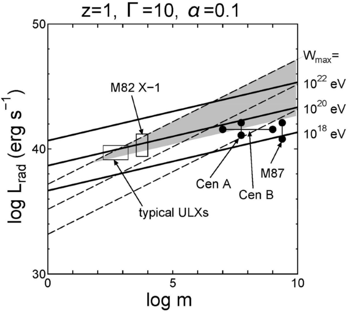

  

  The lines for the maximum energy gain, $W_{\max } = 10^{18}$, $10^{20}$, $10^{22}$ eV, are plotted in $m - L_{{{\text{rad}}}}$ diagram. M82 X-1 is located well above the line of $10^{20}$ eV so that be a good candidate for northern (Abbasi and Abe 2014). Other nearby AGNs, such as M87, Cen A and B, and typical ULXs are also possible candidates of UHECRs ($> 3.9 \times 10^{19} {\text{eV}}$) Grey area ($W_{{\max}} > 3.9 \times 10^{19}$ eV and $\dot{m} < 0.1$) represents possible acceleration region of UHECR. Three dashed lines are for $\dot{m}$ = 10^–5, 10^–3, and 10^–1

• 2. The electrons are also accelerated by the bow wakefield exactly the same way as protons. They emit gamma-ray photons through the interaction with electromagnetic perturbations (Table 7).

• 3. The accretion of charged particles and emission of gamma-rays show prominent variabilities with the various time scales shown in Table 7 due to the accretion instabilities.

• 4. The bow wake acceleration theory can provide the flux estimates in UHECRs, gamma-rays, and neutrinos, which will be compared quantitatively with the recent observational results obtained by ground and space observatories.

Table 7 Time scales, maximum energy, and luminosities

7 High density wakefields and applications to medicine

The recent invention of the coherent addition of fiber lasers (CAN: Coherent Amplification Network) (Mourou et al. 2013) may allow us to consider extremely compact (but in low energy) LWFA accelerators and their new applications. For example, such an accelerator may be employed in an intraoperative radiation therapy (IORT) (Giulietti 2016) and even an endoscopic radiation therapy (ESRT). For these applications we realize that energy of accelerated electrons should be much less than the equivalent accelerator that driven electrons from outside of a patient’s body, as these electrons need not penetrate the substantial thickness of the tissue. If the electron penetration is only for the surface of the organ that shows tumor by inserting the endoscopy to the very spot, the energy range of electrons should be on the order of mere mm. In the following we consider such low energy ultracompact LWFA possibility, and therefore, we explore the high density LWFA. In this case the phase velocity of the wakefield becomes low and it begins to show the phenomenon of sheath. See Table 2.

In the regime of high plasma density, the typical physics of LWFA becomes somewhat modified. In particular near the critical plasma density, the laser group velocity $v_{{\text{g}}} = c\sqrt {1 - n_{{\text{e}}} /n_{{\text{c}}} }$ approaches zero, and the pump depletion and dephasing lengths, which are on the order of $L_{{\text{d}}} \sim L_{{\text{p}}} \sim \lambda_{{\text{p}}} a_{0}^{2} \left( {n_{{\text{c}}} /n_{{\text{e}}} } \right)$, become shorter than the plasma wavelength $\lambda_{{\text{p}}} = 2\pi c/\omega_{{\text{p}}}$ for $a_{0} = 1$. Consequently the laser-plasma interaction primarily occurs within one $\lambda_{{\text{p}}}$, and the laser couples significantly to the bulk motion of the plasma. This situation contrasts starkly with that of low-density wakefield physics, in which the laser penetrates deeply into the plasma without coupling to the bulk motion (having $v_{{\text{g}}} \approx c$). In this case the phase velocity of the wakefield becomes $v_{{{\text{ph}}}} = v_{{\text{g}}} \approx c$, allowing the laser to build a long wake train $\left( {L_{{\text{d}}} \sim L_{{\text{p}}} \gg \lambda_{{\text{p}}} } \right)$ robustly and stably. When electron injection occurs, the wakefield can then skim a small population of electrons from the bulk and accelerate them to high energies.

We may now take a closer look at each regime. The case of sufficiently underdense plasma such as $n_{{\text{c}}} /n_{{\text{e}}} = 10$, the wakefield development is well known. The train of accelerated electrons are clearly visible and the highest-energy electrons reach the theoretically expected momentum of $p_{x}^{\max } \approx m_{{\text{e}}} c\sqrt {(2g\left( {a_{0} } \right)n_{{\text{c}}} /n_{{\text{e}}} )^{2} - 1}$ (Tajima 2010). The coherent wake structure is also seen, with saturation in the longitudinal field reaching the expected value (Mako and Fisher 1979) of $E_{\max } /E_{{{\text{TD}}}} \approx 0.4$. The wake is gradually diminished, as it imparts energy to the electrons, but recovers after the dephasing length $L_{{\text{p}}} \approx 8\lambda_{{\text{p}}}$.

In contrast the case of $n_{{\text{e}}} = n_{{\text{c}}}$, shown in an initial stage in Fig. 28a and final stage in Fig. 28b, exhibits quite different behavior. This is because the physics of the high phase velocity that we have discussed in Sect. 1 (Table 2) has now morphed into that of the low phase velocity regime (the left column of Table 2). In that regime instead of wake excitation with high phase velocity, we now get back to the sheath exciation and its dynmaics, which we encountered before we embarked from the consideration by Esirkepov et al. (2004) and Bulanov et al. (1994). Here, $v_{{\text{g}}} = 0$, and $L_{{\text{p,d}}} \lesssim \lambda_{{\text{p}}}$, restricting the laser-plasma interaction to within one plasma wavelength. The long train of trapped electrons becomes replaced by streams of low-energy (${\Delta }\varepsilon \sim 100 {\text{keV}}$) electrons ejected from the site of oscillation roughly every plasma period. This behavior is somewhat reminiscent of laser interaction with a solid target in that electrons are sprayed forward. However, here the laser is still able to propagate through the target, and the ions have essentially no response.

Fig. 28

High density laser wakefield acceleration process at a very early first and second “fingers” of electrons in the phase space formed by the snapping of the sheath b later after multiple of sheath oscillations. The case of $n_{{\text{c}}} /n_{{\text{e}}} = 1$ (“black”) with $a_{0} = 1$, showing the development of the electron streams. a is zoomed to $0 \le x \le \lambda_{p}$ for clarity (Nicks et al. 2019)

The mechanics of acceleration in the case of $n_{{\text{c}}} /n_{{\text{e}}} \approx 1$ are somewhat different than in the typical wakefield case of $n_{{\text{c}}} /n_{{\text{e}}} \gg 1$. Having $v_{{\text{g}}} \ll c$, the laser couples strongly to the bulk motion of the electrons upon entering the plasma, pushing out a much larger spike in electron density $\left( {\delta n_{{\text{e}}} /n_{{\text{e}}} \approx 3.5} \right)$ than in the low-density case. This density spike creates a longitudinal electric field of approximately twice the strength as in the low-density case and causes the reflection of a substantial portion of the laser. This powerful initial kick to the plasma establishes a strong longitudinal oscillation of electrons in the range $0 \le x \le \lambda_{{\text{p}}}$.

As this initial density spike rebounds, those electrons having $v_{x} \ll c$ are immediately accelerated to near the expected energy from wakefield theory. For subsequent oscillations, the longitudinal field roughly reaches the same saturation amplitude as in the low-density case. Each of these subsequent oscillations accelerates a stream of electrons to low energy $( < 100 {\text{keV}})$ that is then ejected forward from the site of oscillation. Figure 28a, a snapshot of the electron phase space and fields zoomed to the range $0 \le x \le \lambda_{{\text{p}}}$, shows the beginning of this process, where the first streams of accelerated electrons, as well as secondary, fin-like streams, are visible. As the oscillation continues, more streams accumulate, building up the phase-space distribution in Fig. 28b, which shows the full simulation domain. In the later stages, the electron acceleration becomes increasingly turbulent until the oscillation is finally exhausted after about 30 plasma periods. While the individual energy of the accelerated electrons is low compared to that of the low-density case, the total energy imparted to the accelerated electrons can potentially be higher. This total imparted energy represents about 12% of the total injected laser energy. This understanding of the electron dynamics associated with sheath formation (Nicks, et al. 2019; Mako and Tajima 1984) should also be useful for the understanding of related ion acceleration dynamics (Tajima et al. 2017).

In the present setup, where the laser injected from vacuum, a sheath develops that directs the electron streams solely in the forward direction after the initial oscillation. However, if the laser is instead initialized inside the plasma, the same basic behavior of longitudinal oscillation and electron streams are seen, though with some directed in the backward direction. Thus the vacuum injection scheme used here may provide a more experimentally realistic setup for $v_{{\text{g}}} \ll c$ physics without substantially altering the desired physics itself.

The interaction of the laser with the plasma in these two different density regimes has a convenient analogy in tsunami waves in a certain property of the wave dynamics. In the open ocean, where the water depth is great, tsunami waves propagate with a fast phase velocity and thus do not couple to stationary objects. Boats in the ocean, for instance, may move slightly in the transverse direction (vertically), but are not otherwise affected. Near the shore, however, the increasingly shallow water causes the phase velocity of the wave to slow down (the shallow water dispersion is given by its phase velocity v_ph = (gh)^1/2, where g is the gravitational acceleration and h is the water depth, while the deep water has v_ph = (g/k)^1/2 for the wave with wavenumber k) (Lamb 1945), which leads to amplification and steepening of the wave until breaking occurs. We have reviewed this in Sect. 1 (such as in Figs. 1 and 2). The slow velocity of the wave near the shore then causes strong (catastrophic in case of tsunami) “trapping” of stationary objects. Additionally the slow wave velocity couples with turbulence created by wave breaking to create anomalous transport on the sediment bed. Significant amounts of sediment quickly pass into the wave, creating a visibly “black” tsunami from the clean, “blue”, off-shore starting wave. As a further consequence of turbulence, anomalous viscosity causes momentum transport of the sediment. Somewhat analogous to the above described tsunami transformation with respect to the phase velocity in the case of a typical wakefield with $n_{{\text{c}}} \gg n_{{\text{e}}}$, the bulk plasma remains almost entirely unaffected, leaving the wave “blue”. In the high-density case, however, the wave phase velocity becomes sufficiently low to begin scraping particles from the bulk distribution, resulting in “black” waves such as is shown in the phase-space distribution in Fig. 28b. Between these two extremes, a “grey” wave state can exist. This electron dynamics exciting sheath is not so differnt from that observed in CAIL process, in which electrons are driven by sheath (Tajima and Habs 2009).

The penetration depth in human tissue can be approximated by integrating the stopping power of electrons in water, giving the stopping distance in the continuous slowing-down approximation (Berger 1992). At the critical density, the distribution of low-energy electrons has the energy distribution shown in Fig. 29. This distribution $f\left( \varepsilon \right)$ corresponds to a maximum penetration depth $x_{{{\text{CSDA}}}}$ in water of about $\lesssim 1$ cm, as is shown in Fig. 29 as a function of $x_{{{\text{CSDA}}}}$. This result thus represents the lower end of possible penetration depth. Tuning the plasma density allows control of the penetration depth. For $n_{{\text{c}}} /n_{{\text{e}}} = 5$, the electrons produced are somewhat more energetic, and a large population can reach a penetration depth of 1 cm. At $n_{{\text{c}}} /n_{{\text{e}}} = 10$, the maximum range is on the order of centimeters. The laser intensity $a_{0}$ can also be tuned for the desired electron energies produced. As an additional benefit, near the critical density, a significant acceleration of the bulk population of electrons occurs, potentially creating a far larger overall dose of radiation than would occur for more typical wakefield acceleration. The combination of a large dose close to the desired target may be particularly desirable for endoscopic medical applications.

Fig. 29

Sheath oscillations and the penetration spectrum of electrons in the “black tsunami” regime (after Nicks et al. 2019). Shown also is the black tsunami wave on shore (after Nicks et al. 2019)

In absolute terms, the critical density for a 1-micron laser is approximately $10^{21}$ cm⁻³. To achieve such a density, and to avoid the use of gas ionization inside the body, one possibility is porous nanomaterials, such as carbon nanotubes (Tajima 2014). Such a medium would also provide the benefit of guiding the laser. It might also be possible to tailor the design of the nanomaterial to suit the desired plasma density.

8 The future directions

Though materials science and technology may be very important as part of LWFA applications, here we focus on medical applications. The intense laser technology has given a new set of impetus to make innovations in nuclear medicine and pharmacology, not to speak in the broader medicine at large. Our applications to medicine are enabled on our discussions from Sect. 5 (ions beams) and Sect. 7 (electron beams).

As a direct application of LWFA electrons, we recognize the use of LWFA ultrashort electron pulses (compared with electron bunches of conventional accelerators) for ultrafast radiology. Crowell et al (2004) as well as Brozek-Pluskab et al. (2005) have applied LWFA electrons to ultrafast radiolysis. Richter et al. (2011) have irradiated LWFA created electrons on in vitro cells. X-rays emitted by betatron oscillations in LWFA (Corde and Phuoc 2013; Albert and Anderson 2010; Farinella and Lau 2016) may be also employed for diagnosis such as phase contrast imaging (Kneip and McGuffey 2011). Their direct use of LWFA electrons as therapy applications include the intraoperative radiation therapy (IORT) (Giulietti and Bourgeois 2008) and even endoscopic radiation therapy (ESRT). This approach takes advantage of the compactness of the electron source for the surgeon, while he can avoid the surface tissue damage due to the electron’s higher dose at the entrance by opening the organ with tumor during the operation. These applications are well reviewed in the latest book (Giulietti 2016), so that we need not to delve into these topics here further.

The laser wakefield acceleration introduced several fundamentally novel philosophies and principles in both accelerator physics and plasma physics, as described in Sect. 1. Some of the principles such as the employment of an already broken material of plasma as a medium was inherited from the bold research by such pioneers as Veksler and Rostoker, while ameliorating the instabilities arising in plasmas by the principle of high phase velocity and that of a fs ultrafast laser driver. The other pillars of philosophy such as the resonance of the eigenmodes and the relativistic coherence reinforced the large accelerating gradient and its coherent maintenance. It amounted to a bold step forward to climb the ever higher frequency of the driving electromagnetic wave from the RF range to the optical laser range some several orders by a single stroke. As we have seen in Sect. 2, we are about to witness another quantum jump by several orders in the driver’s frequency from optical laser to X-ray laser. This would open up a new avenue of research in wakefield acceleration by X-ray laser in crystals or nanostructures. Such may serve as a new class of particle accelerators for high energy research (Chattopadhay et al. 2019). On the other hand, there will be new genre of applications. This is in part due to the invention of the high repetition, high efficiency fiber laser emergence (CAN) (Mourou et al. 2013). Among many possibilities we would like to pick a recent exciting development of its application to laser-driven (relatively low energy) ion acceleration to induce fusion, which in turn drive fission processes of transmutation of spent nuclear waste (Tajima et al. 2018).

8.1 CAN laser driven transmutator

One such application is the neutron generation to transmute and incinerate the spent nuclear fuel to shorten the needed storage from 300,000 to 300 years and to reduce the needed storage volume by factor of 100. So far the high level radioactive nuclear waste poses a serious technical, societal, and financial problem. Even though the human society has been benefitted from the nuclear energy since E. Fermi succeeded the Chicago pile during the World War II time (a “kitchen” side of success in nuclear energy), we have not found a solution to the “toilet” of such nuclear waste. We suggest to generated 14 MeV DT fusion neutrons from T(d,n)He reaction using $a_{0} \approx 1$ CAIL regime. Ejected deuteron with an average energy of 150 keV are then allowed to interact with a tritium target, emitting copious amounts of neutrons. (This should serve a much more compact neutron generator than an alternative ADS (Accelerator Drive System), while the neutron sources are also distributed spatially. The incineration and transmutation of the spent nuclear fuel then proceed by coupling these neutrons to a sub-critical assembly composed of the transuranic elements dissolved in the LiF-BeF₂ eutectic molten salt. The copious and efficient neutron generation may be enabled by the Coherent Amplification Network (CAN) fiber laser concept coupled with high repetition.

The combination of (a) the CAIL-mediated neutron generation driven by CAN laser with (b) the transparent molten salt transmutator should usher in a safe, relatively compact operation, as the liquid operation with laser has many advantages that the past nuclear facilities did not possess. This includes the possibilities of the compactness and distributedness of the neutron generators, real-time monitoring and control, liquid’s inherent negative thermal coefficient for safety, continuous feeding of the transuranic wastes as well as continuous separation of fission products, while in operation, coordinated energy convergence from transmutation, etc. Such a transmutator operation could serve to incinerate wastes from about 10 large scale nuclear reactors in operation.

8.2 TeV on a chip

The invention of the TFC combined with the relativistic compression (RC) brings us a new powerful tool of X-rays, a single-cycled intense X-ray laser, as discussed in Chaps. II and IV. The scaling of LWFA dictates that with high energy X-ray photons the critical density n_cr increases by many orders of magnitude, allowing us to take even solid density electrons as an accelerating media (nanostructured materials, for example) (Tajima 2014; Shin 2014; Zhang and Tajima 2016). The adoption of nanostructured materials is a creative integration of (1) high density (solid density) media for LWFA and (2) an evacuated hole for accelerated particle that also focuses wakefields (Zhang and Tajima 2016). An exploratory research shows a remarkable clean wakefields excited at this solid density medium at the intensity of TeV/cm, opening up a “TeV on a chip” possibility. See Fig. 30. Of course, such a radical concept needs to be tested in experimental investigations. Of particular importance is the realization of the X-ray laser driver.

Fig. 30

Wakefields by a few-cycled 1 keV X-ray pulse (a₀ ~ O(1)), causing 10 TeV/m electric fields in the holed nanostructure (above) more strongly confined in the tube compared with the uniform solid case below (Zhang and Tajima 2016)

While our wish is to serve such accelerators as a component of a future high energy accelerator (collider), we may also use this for a non-luminosity paradigm of high energy particle experiments. This is because the luminosity is required for a collider, and its requirements make the accelerator device in higher energies ever more expensive. On the other hand, if we can remove the requirement of the luminosity, the necessary condition would be greatly reduced. As an example, let us suggest a PeV acceleration of electrons to explore string theoretic vacuum texture (Tajima et al. 2011). The “TeV on a chip” accelerator made up of nanostructures driven by X-ray laser via the TFC and RC from optical laser pulses could compose as an element toward a PeV train.

8.3 Conclusions

Sometime we can directly use the laser instead of exciting wakefields. We can list some such possibilities for the reader to explore such. Because of the CAN laser’s high fluence, we may be able to explore the four beam crossing of specific energy lasers to “sandwich” dark matter candidate of axions (Fujii and Homma 2011). The recent phase stable 10PW class lasers (Geng and Ji 2019) allow us to glimpse into a coherent adding of such laser pulses in a certain specific way to reach 100PW laser pulse (perhaps with TFC combined). This level of laser could begin to make so strong laser acceleration of electrons (“violent acceleration”) whose acceleration amounts to cause the Unruh radiation an equivalent to the Hawking radiation via Einstein’s Equivalence Principle in General Theory of Relativity (Chen and Tajima 1999). This would be the first ever detection of general relativistic laboratory creation and detection of phenomena. The recent suggestion of the observation in nuclear anomaly and its possible interpretation as a discovery of a “fifth force” (Feng and Fornal 2016) may be explored by reversing its process by injecting the energy specific gamma photons with a large fluence (Hakimi, et al. 2019). Such a gamma photon flux may be producible by the laser Compton gamma rays via CAN.

The emergence of laser wakefield acceleration has, on one hand, driven the laser technology to enable its promised land by spurting intense laser technology such as CPA (1985), CAN (2013), TFC (2014), RC (2006). On the other hand, these developments in turn made the realization of the LWFA possible in an increasingly sophisticated fashion as well as its applications to be broad and with still expanding vista. These developments further spurred the establishment of a new scientific field of High Field Science [This was partially an attempt to answer a question posed at the time of the demise of the SSC (Nakajima and Kawakubo 1994)]. Because of this promise there have occurred many high field science labs in the world, to list several example of which: APRC (Advanced Photon Research Center and Kansai Photon Research Institute) of JAERI (Takuma 1996), APRI (Advanced Photon Research Institute (Korea), ELI (Extreme Light Infrastructure) (three campuses of ELI-ALPS, ELI-Beams, ELI-NP) (Tajima et al. 2009), XLS (Extreme Light Station at SIOM) (Tajima and Li 2018). These research activities no doubt further stimulate this already very exciting field further forward in the future.

References

M. Aaboud, G. Aad et al., Performance of top-quark and W-boson tagging with ATLAS in Run 2 of the LHC. Eur. Phys. J. C 79, 375 (2019)
R. Abbasi, M. Abe et al., Indications of intermediate-scale anisotropy of cosmic rays with energy greater than 57 EeV in the northern sky measured with the surface detector of the telescope array experiment. Astrophys. J. Lett. 790, L21 (2014)
F. Albert, S. Anderson et al., Characterization and applications of a tunable, laser-based, MeV-class Compton-scattering γ-ray source. Phys. Rev. Spec. Top. Accel. Beams 13, 070703 (2010)
K. Asada, M. Nakamura, The structure of the M87 jet: a transition from parabolic to conical streamlines. Astrophys. J. Lett 745, L28 (2012)
M. Ashour-Abdalla, J. Leboeuf et al., Ultrarelativistic electromagnetic pulses in plasmas. Phys. Rev. A. 23, 1906 (1981)
S.A. Balbus, J.F. Hawley, A powerful local shear instability in weakly magnetized disks. 1. Linear analysis. Astrophys. J 376, 214–222 (1991)
M. Berger, ESTAR, PSTAR, and ASTAR: Computer programs for calculating stopping-power and range tables for electrons, protons, and helium ions (1992)
J.M. Berger, W.A. Newcomb et al., Heating of a confined plasma by oscillating electromagnetic fields. Phys. Fluids 1, 301–307 (1958)
M. Borghesi, D.H. Campbell et al., Electric field detection in laser-plasma interaction experiments via the proton imaging technique. Phys. Plasmas 9, 2214–2220 (2002)
R. Brinkmann, N. Delbos et al., Chirp mitigation of plasma-accelerated beams by a modulated plasma density. Phys. Rev. Lett. 118, 214801 (2017)
B. Brozek-Pluska, D. Gliger et al., Direct observation of elementary radical events: low- and high-energy radiation femtochemistry in solutions. Radiat. Phys. Chem 72, 149–157 (2005)
S.V. Bulanov, N.M. Naumova, F. Pegorard, Vacuum heating of electron and ion-acceleration in ultrashort laser-pulse interaction with plasma. Plasma Phys. Rep. 20, 574–582 (1994)
S.V. Bulanov, V.A. Vshivkov et al., Laser acceleration of charged particles in inhomogeneous plasmas. Plasma Phys. Rep. 23, 259–269 (1997)
S.V. Bulanov, T.Z. Esirkepov et al., Oncological hadrontherapy with laser ion accelerators. Phys. Lett. A 299, 240–247 (2002)
S. Bulanov, T. Esirkepov, T. Tajima, Light intensification towards the Schwinger limit. Phys. Rev. Lett. 91, 085001 (2003)
S. Busold, D. Schumacher et al., Towards highest peak intensities for ultra-short MeV-range ion bunches. Sci. Rep. UK 5, 12459 (2015)
A. Caldwell, K. Lotov, A. Pukhov, F. Simon, Proton-driven plasma-wakefield acceleration. Nature Phys 5, 363 (2009)
N.E. Canac, K.N. Abazajian, T. Tajima, T. Ebisuzaki, S. Horiuchi, Observational signatures of the gamma ray from bright blazars and wakefield theory. Submitted to MNRAS, 2019. arXiv:1709.06535.
A.W. Chao, K.H. Mes, M. Tigner, F. Zimmermann, Handbook of accelerator physics and engineering (World scientific, Singapore, 2014)
S. Chattopadhay, G. Mourou, V. Shiltsev, T. Tajima (eds.), Crystals and nanostructures (World Scientific, Singapore, 2019)
P.S. Chen, G. Mourou, Accelerating plasma mirrors to investigate the black hole information loss paradox. Phys. Rev. Lett. 118, 045001 (2017)
P.S. Chen, T. Tajima, Testing Unruh radiation with ultraintense lasers. Phys. Rev. Lett. 83, 256–259 (1999)
P. Chen, J. Dawson, R.W. Huff, T. Katsouleas, Acceleration of electrons by the interaction of a bunched electron beam with a plasma. Phys. Rev. Lett. 54, 693 (1985)
P. Chen, T. Tajima, Y. Takahashi, Plasma wakefield acceleration for ultrahigh-energy cosmic rays. Phys. Rev. Lett. 89, 161101 (2002)
M. Chen, A. Pukhov, Z.M. Sheng, X.Q. Yan, Laser mode effects on the ion acceleration during circularly polarized laser pulse interaction with foil targets. Phys. Plasmas 15, 113103 (2008)
P.M. Chesler, L.G. Yaffe, Stress-energy tensor of a quark moving through a strongly-coupled N = 4 supersymmetric Yang–Mills plasma: comparing hydrodynamics and AdS/CFT duality. Phys. Rev. D78 (2008)
C. Cohen-Tannoudji, C. Robilliard, Wave functions, relative phase and interference for atomic Bose–Einstein condensates. Cr Acad Sci IV-Phys 2, 445–477 (2001)
S. Corde, K.T. Phuoc et al., Femtosecond X rays from laser-plasma accelerators. Rev. Mod. Phys. 85, 1–48 (2013)
R.A. Crowell, D.J. Gosztola et al., Ultrafast processes in radiation chemistry. Radiat. Phys. Chem 70, 501–509 (2004)
A. Dopp, E. Guillaume et al., Energy boost in laser wakefield accelerators using sharp density transitions. Phys. Plasmas 23, 056702 (2016)
A. Dopp, C. Thaury et al., Energy-chirp compensation in a laser wakefield accelerator. Phys. Rev. Lett. 121, 074802 (2018)
T. Ebisuzaki, T. Tajima, Astrophysical ZeV acceleration in the relativistic jet from an accreting supermassive blackhole. Astropart Phys 56, 9–15 (2014a)
T. Ebisuzaki, T. Tajima, Pondermotive acceleration of charged particles along the relativistic jets of an accreting blackhole. Eur Phys J-Spec Top 223, 1113–1120 (2014b)
N.A. Ebrahim, C. Joshi, H.A. Baldis, Electron acceleration below quarter-critical density in CO2 laser-produced plasmas. Phys. Lett. A 84, 253–255 (1981)
E. Esarey, C.B. Schroeder, W.P. Leemans, Physics of laser-driven plasma-based electron accelerators. Rev. Mod. Phys. 81, 1229–1285 (2009)
T. Esirkepov, M. Borghei, S.V. Bulanov et al., Highly efficient relativistic-ion generation in the laser-piston regime. Phys. Rev. Lett. 92, 175003 (2004)
T. Esirkepov, M. Yamagiwa, T. Tajima, Laser ion-acceleration scaling laws seen in multiparametric particle-in-cell simulations. Phys. Rev. Lett. 96, 105001 (2006)
T.Z. Esirkepov, Y. Kato, S. Bulanov, Bow wave from ultraintense electromagnetic pulses in plasmas. Phys. Rev. Lett. 101, 265001 (2008)
D.M. Farinella, C.K. Lau et al., High energy photon emission from wakefields. Phys. Plasmas 23, 073107 (2016)
J. Faure, Y. Glinec et al., A laser-plasma accelerator producing monoenergetic electron beams. Nature 431, 541–544 (2004)
J.L. Feng, B. Fornal et al., Protophobic fifth-force interpretation of the observed anomaly in Be-8 nuclear transitions. Phys. Rev. Lett. 117, 071803 (2016)
E. Fermi, Galactic magnetic fields and the origin of cosmic radiation. Astrophys. J 119, 1–6 (1954)
D.L. Fisher, T. Tajima, Superluminous laser-pulse in an active medium. Phys. Rev. Lett. 71, 4338–4341 (1993)
D.L. Fisher, T. Tajima, Enhanced Raman forward scattering. Phys. Rev. E 53, 1844–1851 (1996)
Y. Fujii, K. Homma, An approach toward the laboratory search for the scalar field as a candidate of dark energy. Prog. Theor. Phys 126, 531–553 (2011)
C.G.R. Geddes, C. Toth et al., High-quality electron beams from a laser wakefield accelerator using plasma-channel guiding. Nature 431, 538–541 (2004)
X.S. Geng, L.L. Ji et al., Quantum reflection above the classical radiation-reaction barrier in the quantum electro-dynamics regime. Commun. Phys. 2, 66 (2019)
A. Giulietti, Laser-driven particle acceleration towards radiobiology and medicine (Springer, Berlin, 2016)
A. Giulietti, N. Bourgeois et al., Intense γ-ray source in the giant-dipole-resonance range driven by 10-TW laser pulses. Phys. Rev. Lett. 101, 105002 (2008)
E. Goulielmakis, Z.H. Loh et al., Real-time observation of valence electron motion. Nature 466, 739–U737 (2010)
D. Grischkowsky, A.C. Balant, Optical pulse-compression based on enhanced frequency chirping. Appl. Phys. Lett. 41, 1–3 (1982)
E. Guillaume, A. Dopp et al., Electron rephasing in a laser-wakefield accelerator. Phys. Rev. Lett. 115, 155002 (2015)
S. Hakimi, X.M. Zhang et al., X-ray laser wakefield acceleration in a nanotube, in Beam acceleration in crystals and nanostructures, ed. by S. Chattopadhay, G. Mourou, V. Shiltsev, T. Tajima (World Scientific, Singapore, 2019)
K. Harres, I. Alber et al., Beam collimation and transport of quasineutral laser-accelerated protons by a solenoid field. Phys. Plasmas 17, 023107 (2010)
J.F. Hawley, S.A. Balbus, A powerful local shear instability in weakly magnetized disks. 2. Nonlinear evolution. Astrophys. J. 376, 223–233 (1991)
B.M. Hegelich, B.J. Albright et al., Laser acceleration of quasi-monoenergetic MeV ion beams. Nature 439, 441–444 (2006)
A. Henig, S. Steinke et al., Radiation-pressure acceleration of ion beams driven by circularly polarized laser pulses. Phys. Rev. Lett. 103, 245003 (2009)
J.V. Hernandez, A. Vannucci et al., Neural network prediction of some classes of tokamak disruptions. Nucl. Fusion 36, 1009–1017 (1996)
I. Hofmann, Performance of solenoids versus quadrupoles in focusing and energy selection of laser accelerated protons. Phys. Rev. Spec. Top. Ac 16, 041302 (2013)
I. Hofmann, Review of accelerator driven heavy ion nuclear fusion. Matter Radiat. Extrem. 3, 1–11 (2018)
I. Hofmann, J. Meyer-ter-Vehn et al., Collection and focusing of laser accelerated ion beams for therapy applications. Phys. Rev. Spec. Top-Ac 14, 031304 (2011)
K.M. Hofmann, S. Schell, J.J. Wilkens, Laser-driven beam lines for delivering intensity modulated radiation therapy with particle beams. J. Biophotonics 5, 903–911 (2012)
R.H. Hu, H.Y. Lu et al., Brilliant GeV electron beam with narrow energy spread generated by a laser plasma accelerator. Phys. Rev. Accel. Beams 19, 091301 (2016)
M.S. Hur, H. Suk, Numerical study of 1.1 GeV electron acceleration over a-few-millimeter-long plasma with a tapered density. Phys. Plasmas 18, 033102 (2011)
J.D. Jackson, Classical electrodynamics, 3rd edn. (Wiley, New York, 1998)
D. Jahn, D. Schumacher et al., First application studies at the laser-driven LIGHT beamline: Improving proton beam homogeneity and imaging of a solid target. Nucl. Instrum. Meth. A 909, 173–176 (2018)
M. Kando, Y. Fukuda, A.V. Pirozhkov et al., Demonstration of laser-frequency upshift by electron-density modulations in a plasma wakefield. Phys. Rev. Lett. 99, 135001 (2007)
I.J. Kim. Radiation pressure acceleration of protons with femtosecond petawatt laser pulses. The International Commiittee on Ultrahigh Intensity Lasers (2014)
I.J. Kim, K.H. Pae et al., Radiation pressure acceleration of protons to 93 MeV with circularly polarized petawatt laser pulses. Phys. Plasmas 23, 070701 (2016)
O. Klimo, J. Psikal, J. Limpouch, V.T. Tikhonchuk, Monoenergetic ion beams from ultrathin foils irradiated by ultrahigh-contrast circularly polarized laser pulses. Phys. Rev. Spec. Top. Ac 11, 031301 (2008)
S. Kneip, C. McGuffey et al., X-ray phase contrast imaging of biological specimens with femtosecond pulses of betatron radiation from a compact laser plasma wakefield accelerator. Appl. Phys. Lett. 99, 093701 (2011)
W.H. Knox, R.L. Fork et al., Femtosecond dynamics of resonantly excited excitons in room-temperature gaas quantum wells. Phys. Rev. Lett. 54, 1306–1309 (1985)
W.L. Kruer, K. Estabrook, Jxb heating by very intense laser-light. Phys. Fluids 28, 430–432 (1985)
H. Lamb, Hydrodynamics, vol. 8 (Dover Publications, New York, 1945)
C.K. Lau, P.C. Yeh et al., Ponderomotive acceleration by relativistic waves. Phys. Rev. Spec. Top-Ac 18, 024401 (2015)
W. Leemans, W. Chou, M. Uesaka, Beam Dyn. Newslett. (2011)
Y.T. Li, Z.M. Sheng et al., Demonstration of bulk acceleration of ions in ultraintense laser interactions with low-density foams. Phys. Rev. E 72, 066404 (2005)
G.Q. Liao, Y.T. Li et al., Proton radiography of magnetic fields generated with an open-ended coil driven by high power laser pulses. Matter. Radiat. Extrem. 1, 187–191 (2016)
U. Linz, J. Alonso, What will it take for laser driven proton accelerators to be applied to tumor therapy? Phys. Rev. Spec. Top-Ac 10, 094801 (2007)
U. Linz, J. Alonso, Laser-driven ion accelerators for tumor therapy revisited. Phys. Rev. Accel. Beams 19, 124802 (2016)
B.C. Liu, Z.H. He et al., Generation of high-current proton beams with a low energy spread by phase-stable acceleration (PSA). Ieee T Plasma Sci 36, 1854–1856 (2008)
A. Macchi, F. Cattani, T.V. Liseykina, F. Cornolti, Laser acceleration of ion bunches at the front surface of overdense plasmas. Phys. Rev. Lett. 94, 165003 (2005)
A. Macchi, M. Borghesi, M. Passoni, Ion acceleration by superintense laser-plasma interaction. Rev. Mod. Phys. 85, 751–793 (2013)
A.J. Mackinnon, Y. Sentoku et al., Enhancement of proton acceleration by hot-electron recirculation in thin foils irradiated by ultraintense laser pulses. Phys. Rev. Lett. 88, 215006 (2002)
R.M. Magee, A. Necas et al., Direct observation of ion acceleration from a beam-driven wave in a magnetic fusion experiment. Nat. Phys. 15, 281 (2019)
F. Mako, T. Tajima, Collective ion acceleration by a reflexing electron beam: Model and scaling. Phys. Fluids 27, 1815 (1984)
F. Mako, A. Fisher et al., Collective ion acceleration controlled by a gas gradient. IEEE Trans. Nucl. Sci. 26, 4199–4201 (1979)
A. Maksimchuk, S. Gu et al., Forward ion acceleration in thin films driven by a high-intensity laser. Phys. Rev. Lett. 84, 4108 (2000)
J. Maldacena, The large N limit of superconformal field theories and supergravity. Trends Theoret. Phys. II 484, 51–63 (1999)
V. Malka, Laser plasma accelerators. Phys. Plasmas 19, 055501 (2012)
S.P.D. Mangles, C.D. Murphy et al., Monoenergetic beams of relativistic electrons from intense laser-plasma interactions. Nature 431, 535–538 (2004)
U. Masood, M. Bussmann et al., A compact solution for ion beam therapy with laser accelerated protons. Appl. Phys. B-Lasers O 117, 41–52 (2014)
U. Masood, T.E. Cowan et al., A light-weight compact proton gantry design with a novel dose delivery system for broad-energetic laser-accelerated beams. Phys. Med. Biol 62, 5531–5555 (2017)
A.B. Mikhaĭlovskiĭ, Theory of plasma instabilities: instabilities of a homogeneous plasma. Vol. 1 (Consultants Bureau, 1974)
G. Milluzzo, J. Pipek et al., Geant4 simulation of the ELIMED transport and dosimetry beam line for high-energy laser-driven ion beam multidisciplinary applications. Nucl. Instrum. Meth. A 909, 298–302 (2018)
K. Mima, W. Horton, T. Tajima, A. Hasegawa, Y. Ichikawa, T. Tajima, Nonlinear dynamics, and particle acceleration, vol. 27 (AIP, New York, 1991)
S.Y. Mironov, J. Wheeler, R. Gonin, G. Cojocaru, R. Ungureanu, R. Banici, M. Serbanescu, R. Dabu, G. Mourou, E.A. Khazanov, 100 J-level pulse compression for peak power enhancement. Quant. Electron. 47, 173 (2017)
A. Mizuta, T. Ebisuzaki, T. Tajima, S. Nagataki, Production of intense episodic Alfv´en pulses: GRMHD simulation of black hole accretion discs. MNRAS 479, 2534–2546 (2018)
C.I. Moore, A. Ting et al., Measurements of energetic electrons from the high-intensity laser ionization of gases. Phys. Plasmas 8, 2481–2487 (2001)
G. Mourou, T. Tajima, More intense, shorter pulses. Science 331, 41–42 (2011)
G.A. Mourou, T. Tajima, S.V. Bulanov, Optics in the relativistic regime. Rev. Mod. Phys. 78, 309 (2006)
G. Mourou, B. Brocklesby, T. Tajima, J. Limpert, The future is fibre accelerators. Nat Photon. 7, 258–261 (2013)
G. Mourou, S. Mironov, E. Khazanov, A. Sergeev, Single cycle thin film compressor opening the door to Zeptosecond–Exawatt physics. Eur. Phys. J. Speci. Top. 223, 1181–1188 (2014)
K. Nakajima, T. Kawakubo et al., A proof-of-principle experiment of laser wakefield acceleration. Phys. Scripta T52, 61–64 (1994)
K. Nakajima, D. Fisher et al., Observation of ultrahigh gradient electron acceleration by a self-modulated intense short laser-pulse. Phys. Rev. Lett. 74, 4428–4431 (1995)
N. Naumova, J. Nees et al., Relativistic generation of isolated attosecond pulses in a λ3 focal volume. Phys. Rev. Lett. 92, 063902 (2004)
N. Naumova, I. Sokolov et al., Attosecond electron bunches. Phys. Rev. Lett. 93, 195003 (2004)
B.S. Nicks, S. Hakimi, et al., Electron dynamics in the high-density laser-wakefield acceleration regime, submitted to Phys. Rev. Accel. Beams, 2019; A. Necas, T. Tajima et al. Unification of the radiation pressure acceleration and the coherent acceleration of ions by laser, submitted to Phys. Rev. Accel. Beams (2019)
M. Nishiuchi, I. Daito et al., Focusing and spectral enhancement of a repetition-rated, laser-driven, divergent multi-MeV proton beam using permanent quadrupole magnets. Appl. Phys. Lett. 94, 061107 (2009)
M. Nishiuchi, H. Sakaki et al., Measured and simulated transport of 19 MeV laser-accelerated proton bunches through an integrated test beam line at 1 Hz. Phys. Rev. Spec. Top-Ac 13, 071304 (2010)
M. Nisoli, S. DeSilvestri, O. Svelto, Generation of high energy 10 fs pulses by a new pulse compression technique. Appl. Phys. Lett. 68, 2793–2795 (1996)
M. Nisoli, S. DeSilvestri et al., Compression of high-energy laser pulses below 5 fs. Opt. Lett. 22, 522–524 (1997)
S.M. O’Neill, C.S. Reynolds, M.C. Miller, K. Sorathia, Low-frequency oscillations in global simulations of black hole accretion. Astrophys. J. 736, 107 (2011)
M. Okamura, Laser ion source for heavy ion inertial fusion. Matter Radiat. Extrem. 3, 61–66 (2018)
T. O'Neil, Collisionless damping of nonlinear plasma oscillations. Phys. Fluids 8, 2255–3000 (1965)
M. Passoni, V. Tikhonchuk, M. Lontano, V.Y. Bychenkov, Charge separation effects in solid targets and ion acceleration with a two-temperature electron distribution. Phys. Rev. E 69, 026411 (2004)
P.K. Patel, A.J. Mackinnon et al., Isochoric heating of solid-density matter with an ultrafast proton beam. Phys. Rev. Lett. 91, 125004 (2003)
A. Pirozhkov, M. Kando et al., Soft-X-ray harmonic comb from relativistic electron spikes. Phys. Rev. Lett. 108, 135004 (2012)
L. Pommarel, B. Vauzour et al., Spectral and spatial shaping of a laser-produced ion beam for radiation-biology experiments. Phys. Rev. Accel. Beams 20, 032801 (2017)
A. Pukhov, D. An der Bruegge, Enhanced relativistic harmonics by electron nanobunching. Phys. Plasmas 17, 124039 (2010)
A. Pukhov, I. Kostyukov, Control of laser-wakefield acceleration by the plasma-density profile. Phys. Rev. E 77, 025401 (2008)
A.B. Pushkarev, Y. Kovalev, M. Lister, T. Savolainen, MOJAVE–XIV. Shapes and opening angles of AGN jets. Mon. Not. Roy. Astron. Soc. 468, 4992–5003 (2017)
B. Qiao, M. Zepf, M. Borghesi, M. Geissler, Stable GeV ion-beam acceleration from thin foils by circularly polarized laser pulses. Phys. Rev. Lett. 102, 145002 (2009)
B. Rau, T. Tajima, Strongly nonlinear magnetosonic waves and ion acceleration. Phys. Plasmas 5, 3575–3580 (1998)
C. Richter, M. Kaluza et al., Dosimetry of laser-accelerated electron beams used for in vitro cell irradiation experiments. Radiat. Meas. 46, 2006–2009 (2011)
W. Rittershofer, C.B. Schroeder et al., Tapered plasma channels to phase-lock accelerating and focusing forces in laser-plasma accelerators. Phys. Plasmas 17, 063104 (2010)
A.P.L. Robinson, M. Zepf et al., Radiation pressure acceleration of thin foils with circularly polarized laser pulses. New. J. Phys. 10, 013021 (2008)
C. Rolland, P.B. Corkum, Compression of high-power optical pulses. J. Opt. Soc. Am. B 5, 641–647 (1988)
F. Romano, F. Schillaci et al., The ELIMED transport and dosimetry beamline for laser-driven ion beams. Nucl. Instrum. Meth. A 829, 153–158 (2016)
N. Rostoker, M. Reiser, Collective methods of acceleration (Harwood Academic Publishers, New York, 1979)
M. Roth, T.E. Cowan et al., Fast ignition by intense laser-accelerated proton beams. Phys. Rev. Lett. 86, 436–439 (2001)
M. Roth, I. Alber et al., Proton acceleration experiments and warm dense matter research using high power lasers. Plasma. Phys. Contr. F 51, 124039 (2009)
S.G. Rykovanov, J. Schreiber et al., Ion acceleration with ultra-thin foils using elliptically polarized laser pulses. New. J. Phys. 10, 113005 (2008)
S. Schell, J.J. Wilkens, Modifying proton fluence spectra to generate spread-out Bragg peaks with laser accelerated proton beams. Phys. Med. Biol. 54, N459–N466 (2009)
F. Schillaci, L. Pommarel et al., Characterization of the ELIMED permanent magnets quadrupole system prototype with laser-driven proton beams. J. Instrum 11, T07005 (2016)
K. Schmid, A. Buck et al., Density-transition based electron injector for laser driven wakefield accelerators. Phys. Rev. Spec. Top. Accelerators Beams 13, 091301 (2010)
M. Schollmeier, S. Becker et al., Controlled transport and focusing of laser-accelerated protons with miniature magnetic devices. Phys. Rev. Lett. 101, 055004 (2008)
H. Schwoerer, S. Pfotenhauer et al., Laser-plasma acceleration of quasi-monoenergetic protons from microstructured targets. Nature 439, 445–448 (2006)
V. Scuderi, S.B. Jia et al., Development of an energy selector system for laser-driven proton beam applications. Nucl. Instrum. Meth. A 740, 87–93 (2014)
N.I. Shakura, R.A. Sunyaev, Black holes in binary-systems: observational appearance. Astron. Astrophys. 24, 337 (1973)
B.Y. Sharkov, D.H.H. Hoffmann, A.A. Golubev, Y.T. Zhao, High energy density physics with intense ion beams. Matter Radiat Extrem 1, 28–47 (2016)
Z.M. Sheng, K. Mima, J. Zhang, H. Sanuki, Emission of electromagnetic pulses from laser wakefields through linear mode conversion. Phys. Rev. Lett. 94, 095003 (2005)
K. Shibata, T. Tajima, R. Matsumoto, Magnetic accretion disks fall into two types. Astrophys. J. 350, 295–299 (1990)
Y.M. Shin, Beam-driven acceleration in ultra-dense plasma media. Appl. Phys. Lett. 105, 114106 (2014)
R. Snavely, M. Key et al., Intense high-energy proton beams from petawatt-laser irradiation of solids. Phys. Rev. Lett. 85, 2945 (2000)
I. Spencer, K.W.D. Ledingham et al., Laser generation of proton beams for the production of short-lived positron emitting radioisotopes. Nucl. Instrum. Meth. B 183, 449–458 (2001)
P. Sprangle, B. Hafizi et al., Wakefield generation and GeV acceleration in tapered plasma channels. Phys. Rev. E 63, 056405 (2001)
D. Strickland, G. Mourou, Compression of amplified pulses. Opt. Commun. 56, 219–221 (1985)
T. Tajima, High-energy laser plasma accelerators. Laser Part. Beams 3, 351–413 (1985)
T. Tajima, Laser acceleration and its future. Proc. Jpn. Acad. B-Phys. 86, 147–157 (2010)
T. Tajima, Laser acceleration in novel media. Eur. Phys. J. Spec. Top. 223, 1037–1044 (2014)
T. Tajima, Computational plasma physics: with applications to fusion and astrophysics (Addison-Wesley, Reading, 2004)
T. Tajima, J.M. Dawson, Laser electron accelerator. Phys. Rev. Lett. 43, 267 (1979)
T. Tajima, D. Habs, X. Yan. in Reviews of accelerator science and technology: volume 2: medical applications of accelerators, 201–228, ed. by A.W. Chao, U. Chou (World Scientific, 2009)
T. Tajima, R. Li, Marriage of a 20 keV superconducting XFEL with a 100PW laser: a new regime of science at Exawatts and zeptoseconds impacting on the society, SPIE (2018)
T. Tajima, F. Mako, Self-consistent potential for a relativistic magnetized electron beam through a metallic boundary. Phys. Fluids 21, 1459 (1978)
T. Tajima, K. Shibata, Plasma astrophysics (Addison-Wesley, Reading, 1997)
T. Tajima, K. Mima, H. Baldis, High-field science (Springer, Berlin, 2000)
T. Tajima, B. Barish, C.P. Barty, S. Bulanov, P. Chen et al., Science of extreme light infrastrure (Scientific Advisory Committee of Extreme Light Infrastructure, EU, 2009)
T. Tajima, M. Kando, M. Teshima, Feeling the texture of vacuum—laser Acceleration toward PeV. Prog. Theor. Phys.125, 617 (2011). (arXiv:1005.3442v1 [physics.plasm-ph])
T. Tajima, K. Nakajima, G. Mourou, Laser acceleration. Riv Nuovo Cimento 40, 33 (2017)
T. Tajima, A. Necas, G. Mourou, S. Gales, M. Leroy, Fusion triggered liquid-phase transmutator monitored and controlled real-time by CAN laser. Submitted to Fusion Science Technology (2018)
H. Takuma (ed.), The birth and future of quantum photon science: handbook for the generation of a new system of science and technology (Science Tech. Agency of Japan, Tokyo, 1996)
T. Toncian, M. Borghesi et al., Ultrafast laser-driven microlens to focus and energy-select mega-electron volt protons. Science 312, 410–413 (2006)
T. Toncian, M. Amin et al., Properties of a plasma-based laser-triggered micro-lens. AIP Adv 1, 022142 (2011)
V.I. Veksler. Coherent principle of acceleration of charged particles. CERN Symposium on High Energy Acelerators and Pion Physics (1956)
F. Wagner, O. Deppert et al., Maximum proton energy above 85 MeV from the relativistic interaction of laser pulses with micrometer thick CH2 targets. Phys. Rev. Lett. 116, 205002 (2016)
H. Wang, C. Lin et al., Laser shaping of a relativistic intense, short Gaussian pulse by a plasma lens. Phys. Rev. Lett. 107, 265002 (2011)
W.T. Wang, W.T. Li et al., High-brightness high-energy electron beams from a laser wakefield accelerator via energy chirp control. Phys. Rev. Lett. 117, 124801 (2016)
S.M. Weng, Z.M. Sheng et al., Optimization of hole-boring radiation pressure acceleration of ion beams for fusion ignition. Matter Radiat. Extrem. 3, 28–39 (2018)
M. Xie, T. Tajima, K. Yokoya, S. Chattopadhyay, Studies of laser-driven 5 TeV e(+)e(−) colliders in strong quantum beamstrahlung regime. Aip Conf. Proc 398, 233–242 (1997)
X. Yan, C. Lin et al., Generating high-current monoenergetic proton beams by a circularlypolarized laser pulse in the phase-stableacceleration regime. Phys. Rev. Lett. 100, 135003 (2008)
X.Q. Yan, C. Lin et al., Generating high-current monoenergetic proton beams by a circularly polarized laser pulse in the phase-stable acceleration regime. Phys. Rev. Lett. 100, 135003 (2008)
X. Yan, H.-C. Wu et al., Self-organizing GeV, nanocoulomb, collimated proton beam from laser foil interaction at 7 × 10²¹ W/cm2. Phys. Rev. Lett. 103, 135001 (2009)
X. Yan, T. Tajima et al., Theory of laser ion acceleration from a foil target of nanometer thickness. Appl. Phys. B 98, 711–721 (2010)
Y. Yin, W. Yu et al., Influence of target thickness on the generation of high-density ion bunches by ultrashort circularly polarized laser pulses. Phys. Plasmas 15, 093106 (2008)
L. Yin, B.J. Albright et al., Three-dimensional dynamics of breakout afterburner ion acceleration using high-contrast short-pulse laser and nanoscale targets. Phys. Rev. Lett. 107, 045003 (2011)
A. Yogo, T. Maeda et al., Measurement of relative biological effectiveness of protons in human cancer cells using a laser-driven quasimonoenergetic proton beamline. Appl. Phys. Lett. 98, 071304 (2011)
S. Yong, Z. Kun et al., Preliminary design of a laser accelerator beam line. Chin. Phys. C 38, 117011 (2014)
X.M. Zhang, B.F. Shen et al., Efficient GeV ion generation by ultraintense circularly polarized laser pulse. Phys. Plasmas 14, 123108 (2007)
X.M. Zhang, T. Tajima et al., Particle-in-cell simulation of x-ray wakefield acceleration and betatron radiation in nanotubes. Phys. Rev. Accel. Beams 19, 101004 (2016)
S. Zhao, C. Lin et al., Ion acceleration enhanced by target ablation. Phys. Plasmas 22, 073106 (2015)
M.L. Zhou, S. Zhao et al., Instability-free ion acceleration by two laser pulses. Eur. Phys. J. Spec. Top 223, 1031–1035 (2014)
M.L. Zhou, X.Q. Yan et al., Proton acceleration by single-cycle laser pulses offers a novel monoenergetic and stable operating regime. Phys. Plasmas 23, 043211 (2016)
J.G. Zhu, M.J. Wu et al., Experimental demonstration of a laser proton accelerator with accurate beam control through image-relaying transport. Phys. Rev. Accel. Beams 22, 061302 (2019)
Acknowledgements
The first author (TT) acknowledges his gratefulness for the award of the S. Chandrasekhar Prize by the AAPPS-DPP. He humbly cherishes this honor, particularly because some of this work amount to standing on the shoulder of S. Chandrasekhar†, for such topics as black holes (and neutron stars), their structure, and their emanation of wakefields from them. We would like to thank many pioneers and colleagues who contributed to this long journey of investigations by giving us encouragements, guidance, collaboration, and countless helps, including: K. Abazajian, F. Albert, H. Alfven†, H. Azechi, C. Barty, S. Barwick, P. Bolton, M. Borghesi, A. Bracco, B. Brocklesby, P. Bucksbaum, S. Bulanov, R. Byer, A. Caldwell, M. Campbell, A. Chao, S. Chu, L. Cifarelli, S. Chattopadhay, P. Chen, C. Cohen-Tannoudji, S. Corde, P. Corkum, J. Dawson†, S. DeSilvestri, T. Ditmire, F. Dollar, M. Downer, E. Esarey, T. Esirkepov, R. Falcone, J. Faure, J. Feng, M. Fujiwara, S. Gales, A. Giulietti, G. Gulsen, E. Goulielmakis, D. Habs, D. Hammer, T. Hayakawa, M. Hegelich, B. Holzer, K. Homma, W. Horton, S. Ichimaru, S. Iijima, K. Ishikawa, C. Joshi, T. Juhasz, M. Kando, Y. Kato, T. Katsouleas, I. Kim, Y. Kishimoto, A. Krasznahorkay, F. Krausz, K. Krushelnick, A. Lankford, J. Leboeuf, W. Leemans, A. L’Huillier, R. Li, A. Litvak, F. Mako, V. Malka, T. Massard, R. Matsumoto, C. Max, P. McKenna, J. Meyer-ter-Vehn, H. Milchberg, K. Mima, G. Mourou, S. Mukamel, M. Murnane, N. Naumova, K. Nakajima, A. Necas, D. Neely, D. Niculae, A. Olinto, T. O’Neil, F. Pegoraro, A. Pirozhkov, R. Rassmann, B. Richter†, M. Rosenbluth†, J. Rosenzweig, N. Rostoker†, R. Ruth, D. Ryutov, A. J. Shaka, A. Salam†, W. Sandner†, J. Schreiber, A. Sergeev, W. J. Sha, K. Shibata, V. Shiltsev, Y. Shin, Z. Siwy, H. Sobel, M. Spiro, P. Sprangle, D. Strickland, A. Suzuki, P. Taborek, T. Tait, Y. Takahashi†, H. Takuma†, F. Tamonoi, K. Tanaka, M. Teshima, M. Tigner, B. Tromberg, D. Umstadter, C. Wahlstrom, John Wheeler†, Jonathan Wheeler, U. Wienands, T. Yamazaki, K. Yokoya, N. Zamfir, M. Zepf, X. M. Zhang, F. Zimmermann, J. Zuegel, and E. Zweibel. We have been blessed with excellent students and associates who made very close camaraderie during these times and exceptional contributions in the formative years, who include: N. Canac, M. Cavenago, L. M. Chen, S. Cheshkov, A. Deng, D. Farinella, D. Fisher, S. Hakimi, J. Koga, C. Lau, B. S. Nicks, T. Kurki-Suonio, R. H. Hu, A. Mizuta, B. Newberger, M. Ottinger, B. Rau, C. Siders, S. Steinke, X. Z. Wu, and M. Zhou. Our students made dedicated and careful check of our manuscript. It has been a great honor to get involved with all these colleagues throughout this work, without which this work was not completed. The present work was supported by the Norman Rostoker Fund at UCI. XQY was partially supported by National Basic Research Program of China (Grant No. 2013CBA01502), National Natural Science Foundation of China (Grants No. 11921006, No. 11575011).
Author information
Authors and Affiliations
Corresponding author
Additional information
Publisher's Note
Springer Nature remains neutral with regard to jurisdictional claims in published maps and institutional affiliations.
T. Tajima: 2018 recipient of the S. Chandrasekhar Prize.
Rights and permissions
Open Access This article is licensed under a Creative Commons Attribution 4.0 International License, which permits use, sharing, adaptation, distribution and reproduction in any medium or format, as long as you give appropriate credit to the original author(s) and the source, provide a link to the Creative Commons licence, and indicate if changes were made. The images or other third party material in this article are included in the article's Creative Commons licence, unless indicated otherwise in a credit line to the material. If material is not included in the article's Creative Commons licence and your intended use is not permitted by statutory regulation or exceeds the permitted use, you will need to obtain permission directly from the copyright holder. To view a copy of this licence, visit http://creativecommons.org/licenses/by/4.0/.
About this article
Cite this article
Tajima, T., Yan, X.Q. & Ebisuzaki, T. Wakefield acceleration. Rev. Mod. Plasma Phys. 4, 7 (2020). https://doi.org/10.1007/s41614-020-0043-z
Received:
Accepted:
Published:
DOI: https://doi.org/10.1007/s41614-020-0043-z