The reflection distance between zigzag persistence modules

Abstract

By invoking the reflection functors introduced by Bernstein et al. (Russ Math Surv 28(2):17–32, 1973), in this paper we define a metric on the space of all zigzag modules of a given length, which we call the reflection distance. We show that the reflection distance between two given zigzag modules of the same length is an upper bound for the $\ell ^1$-bottleneck distance between their respective persistence diagrams.

Appendices

Appendices

Limits and colimits

We assume the reader is familiar with (small) categories, functors, and natural transformations (see Mac Lane 1971; Riehl 2017 for details). We denote by $\mathbf {Vect}$ the category of vector spaces over some fixed field $\mathbb {F}$.

Definition A1.1

Fix a small category $\mathcal {J}$.

• 1. A diagram of vector spaces of shape$\mathcal {J}$ is a functor $D:\mathcal {J}\rightarrow \mathbf Vect$.

• 2. A cone over a diagram $D:\mathcal {J}\rightarrow \mathbf Vect$ is a vector space N together with a collection of linear transformations $\lambda :=\{\lambda _J: N\rightarrow D(J)\ | \ J\in \text {Ob}(\mathcal {J})\}$, indexed by the objects of $\mathcal {J}$, such that for any morphism $f:A\rightarrow B$ in $\text {Hom}(\mathcal {J})$ we have $\lambda _B = D(f)\circ \lambda _A$. We denote such a cone by $(N,\lambda )$.

• 3. A cocone over a diagram $D:\mathcal {J}\rightarrow \mathbf Vect$ is a vector space M together with a collection of linear transformations $\gamma :=\{\gamma _J: D(J)\rightarrow M \ | \ J\in \text {Ob}(\mathcal {J})\}$, indexed by the objects of $\mathcal {J}$, such that for any morphism $f:A\rightarrow B$ in $\text {Hom}(\mathcal {J})$ we have $\gamma _A = \gamma _B\circ D(f)$. We denote such a cocone by $(M,\lambda )$.

Limits and colimits are then universal cones or cocones, respectively:

Definition A1.2

Let $D:\mathcal {J}\rightarrow \mathbf {Vect}$ be a diagram of vector spaces.

• 1. The limit of the diagram D is a cone $(L,\phi )$ over D such that for any other cone $(N,\lambda )$ over D, there exists a unique linear transformation $\psi :N\rightarrow L$ with $\lambda _A = \phi _A \circ \psi$ for all $A\in \text {Ob}(\mathcal {J})$. We denote the limit L by $\,\lim D$.

• 2. The colimit of the diagram D is a cocone $(C,\phi )$ over D such that for any other cocone $(M,\lambda )$ over D, there exists a unique linear transformation $\psi :M\rightarrow C$ with $\lambda _A = \phi _A \circ \psi$ for all $A\in \text {Ob}(\mathcal {J})$. We denote the colimit C by $\text {colim}(D)$.

Theorem A1.1

Let $\mathcal {J}$ be a small category and let $D^1,D^2$ be diagrams of vector spaces. If there exists a natural transformation $\eta :D^1\rightarrow D^2$ all of whose components are monomorphisms, then $(L^1,\eta _J\circ \lambda ^1_J)$ is a cone for $D^2$ and the unique morphism $\psi :L^1\rightarrow L^2$ satisfying $\eta _J\circ \lambda ^1_J = \lambda ^2_J\circ \psi$ for all $J\in \mathcal {J}$ is a monomorphism.

Proof

The proof can be found in more generality in Borceux et al. (1994 p. 89, Corollary 2.15.3). $\square$

Let $\mathbf {2}$ denote the discrete category with 2 objects. That is, $\text {Ob}(\mathbf {2}) = \{1,2\}$ and $\text {Hom}(1,2) = \emptyset$.

Definition A1.3

Let X, Y be objects in the category $\,\mathcal {C}$ and let $D:\mathbf {2}\rightarrow \mathcal {C}$ be the diagram given by $D(1) = X$ and $D(2) = Y$.

• 1. The product of B and C, denoted $B\times C$, is the limit of D, if it exists,

• 2. The coproduct of B and C, denoted $B\amalg C$, is the colimit of D, if it exists.

In $\mathbf {Vect}$, products and coproducts always exist and coincide.

Theorem A1.2

Let $\mathcal {J}$ be a small category and let $D^1, D^2$ be diagrams of vector spaces. Then $\lim (D^1\times D^2)\cong \lim (D^1)\times \lim (D^2)$ Dually, $\text {colim}(D^1\amalg D^2)\cong \text {colim}(D^1)\amalg \text {colim}(D^2)$. Here $D^1\times D^2$ and $D^1\amalg D^2$ denote the product and coproduct, respectively, of $D^1$ and $D^2$ in the functor category $\mathcal {C}^\mathcal {J}$.

Proof

Consider the product category $\mathbf {2}\times J$ and let $F:\mathbf {2}\times \mathcal {J}\rightarrow \mathcal {C}$ be the functor given by $F(i,j) = D^i(j)$ for $i = 1,2$ and $j\in \mathcal {J}$. By commutativity of limits,

$$\begin{aligned} \lim _\mathbf {2}\lim _\mathcal {J} F(i,j) = \lim _\mathcal {J}\lim _\mathbf {2}F(i,j) \end{aligned}$$

[see Riehl (2017 p. 111, Theorem 3.8.1)]. Now

$$\begin{aligned} \lim (D^1\times D^2)&= \lim _{\mathcal {J}}(D^1\times D^2) = \lim _{\mathcal {J}}\lim _\mathbf {2} F(i,j)\\&= \lim _{\mathbf {2}}\lim _\mathcal {J} F(i,j) = \lim _{\mathbf {2}}\lim D^i\\&= \lim (D^1)\times \lim (D^2). \end{aligned}$$

The second statement follows by a duality argument. $\square$

Matchings

The Matching Lemma is a useful tool for combining matchings in opposite directions into a single matching. For us, the lemma was crucial for proving our stability result, while Bjerkevik makes use of the lemma in proving his generalization of the algebraic stability theorem (Bjerkevik 2016). While it may be one of the earliest results in infinite matching theory (Aharoni 1991), we believe its applications to stability-type questions in persistence theory make it worth expounding upon here.

Lemma A2.1

(Matching lemma for finite matchings) Let S and T be sets and let $f:S\nrightarrow T$ and $g:T\nrightarrow S$ be finite matchings. Then there exists a matching $M:S\nrightarrow T$ such that

• 1. $\text {coim}(f)\subseteq \text {coim}(M)$,

• 2. $\text {coim}(g)\subseteq \text {im}(M)$,

• 3. if $M(s) = t$ then either $f(s) = t$ or $g(t) = s$.

Proof

The proof is inspired by a proof of the Cantor–Schröder–Bernstein theorem³ given in Schweizer (2000). Let $s\in \text {coim}(f)$, $t\in \text {coim}(g)$, and consider sequences of the form

$$\begin{aligned} \cdots {\mathop {\longrightarrow }\limits ^{g}}f^{-1}(g^{-1}(s)){\mathop {\longrightarrow }\limits ^{f}} g^{-1}(s){\mathop {\longrightarrow }\limits ^{g}}s{\mathop {\longrightarrow }\limits ^{f}} f(s) {\mathop {\longrightarrow }\limits ^{g}} g(f(s)) {\mathop {\longrightarrow }\limits ^{f}} \cdots \end{aligned}$$

and

$$\begin{aligned} \cdots {\mathop {\longrightarrow }\limits ^{f}}g^{-1}(f^{-1}(t)){\mathop {\longrightarrow }\limits ^{g}} f^{-1}(t){\mathop {\longrightarrow }\limits ^{f}}t{\mathop {\longrightarrow }\limits ^{g}} g(t) {\mathop {\longrightarrow }\limits ^{f}} f(g(t)) {\mathop {\longrightarrow }\limits ^{g}} \cdots , \end{aligned}$$

where we allow these sequences to terminate to the right or left when undefined. We refer to these sequences as the orbits of s or t. Since f and g are finite matchings, such sequences either terminate on both the left and right, or are infinite but periodic. By injectivity of f and g, every element of $\text {coim}(f)\sqcup \text {coim}(g)$ appears in exactly one orbit. Moreover, every orbit falls into one of the following five classes:

• 1. $s\rightarrow t\rightarrow \cdots \rightarrow s\rightarrow y$,

• 2. $s\rightarrow t\rightarrow \cdots \rightarrow s\rightarrow t\rightarrow x$,

• 3. $t\rightarrow s\rightarrow \cdots \rightarrow t\rightarrow x$,

• 4. $t\rightarrow s\rightarrow \cdots \rightarrow t\rightarrow s\rightarrow y$,

• 5.

  

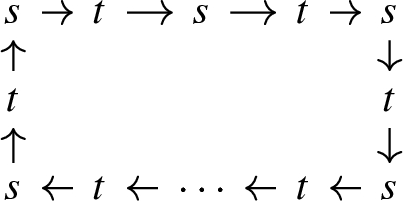
where the s’s and t’s represent elements of $\text {coim}(f)$ and $\text {coim}(g)$, respectively, arrows represent either f or g, and y’s and x’s represent elements of $\text {im}(f){\setminus } \text {coim}(g)$ and $\text {im}(g){\setminus } \text {coim}(f)$, respectively. We define a matching $M:S\nrightarrow T$ as follows: for each $i = 1,\ldots ,5$ let

$$\begin{aligned} S_i^{\text {co}}:= \{s\in \text {coim}(f) \ | \ s \text { appears in an orbit of type } i\} \end{aligned}$$

and

$$\begin{aligned} T_i^{\text {co}}:= \{t\in \text {coim}(g) \ | \ t \text { appears in an orbit of type } i\}. \end{aligned}$$

Then and . We partition $S_1^{\text {co}}$ and $T_3^{\text {co}}$ further by defining

$$\begin{aligned} S_1^{\text {co}\backslash \text {p}} : = \{s\in S_1^{\text {co}} \ | \ f(s)\in \text {coim}(g)\}, \quad S_1^{\text {p}} : = \{s\in S_1^{\text {co}} \ | \ f(s)\not \in \text {coim}(g)\},\\ T_3^{\text {co}\backslash \text {p}} : = \{t\in T_3^{\text {co}} \ | \ g(t)\in \text {coim}(f)\}, \quad \text { and } \quad T_3^{\text {p}} : = \{t\in T_3^{\text {co}}\ | \ g(t)\not \in \text {coim}(f)\}, \end{aligned}$$

so that and . The image, coimage, and mapping of M is specified by the diagram

Note that $f(S_1^{\text {co}\backslash \text {p}}) = T_1^{\text {co}}$, $f(S_2^{\text {co}}) = T_2^{\text {co}}$, $g(T_3^{\text {co}\backslash \text {p}}) = S_3^{\text {co}}$, $g(T_4^{\text {co}}) = S_4^{\text {co}}$, and $f(S_5^{\text {co}}) = T_5^{\text {co}}$ so that M is surjective. Since f and g are injective, we see that M is a bijection between each of the parts specified and thus defines a matching. Moreover, and . Property (3) evidently holds by the definition of M. $\square$

References

Aharoni, R.: Infinite matching theory. Discrete Math. 95(1), 5–22 (1991)
Babichev, A., Morozov, D., Dabaghian, Y.: Robust spatial memory maps encoded by networks with transient connections. PLoS Comput Biol 14(9), e1006433 (2018). https://doi.org/10.1371/journal.pcbi.1006433
Bauer, U., Lesnick, M.: Induced matchings of barcodes and the algebraic stability of persistence. In: Proceedings of the 30th Annual Symposium on Computational Geometry, p. 355. ACM, New York (2014)
Bernstein, I.N., Gel’fand, I.M., Ponomarev, V.A.: Coxeter functors and Gabriel’s theorem. Russ. Math. Surv. 28(2), 17–32 (1973)
Bjerkevik, H.B.: Stability of higher-dimensional interval decomposable persistence modules. ArXiv e-prints (Sept. 2016)
Bjerkevik, H.B., Botnan, M.B., Kerber, M.: Computing the interleaving distance is NP-hard. Preprint (2018). arXiv:1811.09165
Borceux, F., Rota, G.C., Doran, B., Flajolet, P., Lam, T.Y., Lutwak, E., Ismail, M.: Handbook of Categorical Algebra: Volume 1, Basic Category Theory. Cambridge Textbooks in Linguis. Cambridge University Press, Cambridge (1994)
Botnan, M., Lesnick, M.: Algebraic stability of zigzag persistence modules. Algebraic Geom. Topol. 18(6), 3133–3204 (2018)
Bubenik, P., Scott, J.A.: Categorification of persistent homology. Discrete Comput. Geom. 51(3), 600–627 (2014)
Bubenik, P., de Silva, V., Scott, J.: Metrics for generalized persistence modules. Found. Comput. Math. 15(6), 1501–1531 (2015)
Carlsson, G., De Silva, V.: Zigzag persistence. Found. Comput. Math. 10(4), 367–405 (2010)
Chazal, F., Cohen-Steiner, D., Glisse, M., Guibas, L.J., Oudot, S.Y.: Proximity of persistence modules and their diagrams. In: Proceedings of the 25th Annual Symposium on Computational Geometry—SCG’09 (2009)
Chazal, F., De Silva, V., Glisse, M., Oudot, S.: The Structure and Stability of Persistence Modules. Springer, Berlin (2016)
Chowdhury, S., Dai, B., Mémoli, F.: The importance of forgetting: limiting memory improves recovery of topological characteristics from neural data. PLoS ONE 13(9), e0202561 (2018). https://doi.org/10.1371/journal.pone.0202561
Cohen-Steiner, D., Edelsbrunner, H., Morozov, D.: Vines and vineyards by updating persistence in linear time. In: Proceedings of the 22nd Annual Symposium on Computational Geometry, pp. 119–126. ACM, New York (2006a)
Cohen-Steiner, D., Edelsbrunner, H., Harer, J.: Stability of persistence diagrams. Discrete Comput. Geom. 37(1), 103–120 (2006b)
Cohen-Steiner, D., Edelsbrunner, H., Harer, J., Mileyko, Y.: Lipschitz functions have \(L_{p}\)-stable persistence. Found. Comput. Math. 10(2), 127–139 (2010)
Corcoran, P., Jones, C.B.: Spatio-temporal modeling of the topology of swarm behavior with persistence landscapes. In: Proceedings of the 24th ACM SIGSPATIAL International Conference on Advances in Geographic Information Systems, p. 65. ACM, New York (2016)
Delfinado, C.J.A., Edelsbrunner, H.: An incremental algorithm for betti numbers of simplicial complexes on the 3-sphere. Comput. Aided Geom. Des. 12(7), 771–784 (1995)
Edelsbrunner, H., Harer, J.: Computational Topology: An Introduction. American Mathematical Society, New York (2010)
Edelsbrunner, H., Letscher, D., Zomorodian, A.: Topological persistence and simplification. In: 2000. Proceedings. 41st Annual Symposium on Foundations of Computer Science, pp. 454–463. IEEE, New York (2000)
Frosini, P.: A distance for similarity classes of submanifolds of a euclidean space. Bull. Aust. Math. Soc. 42(3), 407–415 (1990)
Frosini, P.: Measuring shapes by size functions. In: Intelligent Robots and Computer Vision X: Algorithms and Techniques, vol. 1607, pp. 122–134. International Society for Optics and Photonics, New York (1992)
Gabriel, P.: Unzerlegbare darstellungen I. Manuscr. Math. 6(1), 71–103 (1972)
Kalisnik, S.: Persistent homology and duality. Ph.D. Thesis. University of Ljubljana (2013)
Kim, W., Memoli, F.: Stable signatures for dynamic metric spaces via zigzag persistent homology. Preprint (2017). arXiv:1712.04064
Lesnick, M.: The theory of the interleaving distance on multidimensional persistence modules. Found. Comput. Math. 15(3), 613–650 (2015)
Mac Lane, S.: Categories for the Working Mathematician. Springer, Berlin (1971)
Ore, O.: Theory of Graphs, vol. 38. American Mathematical Society, New York (1962)
Oudot, S.Y.: Persistence Theory: From Quiver Representations to Data Analysis. American Mathematical Society, New York (2015)
Riehl, E.: Category Theory in Context. Dover Modern Math Originals. Dover Publications, Aurora (2017)
Robins, V.: Towards computing homology from finite approximations. Topol. Proc. 24, 503–532 (1999)
Schweizer, B.: Cantor, Schröder, and Bernstein in orbit. Math. Mag. 73(4), 311 (2000)
Tausz, A., Carlsson, G.: Applications of zigzag persistence to topological data analysis. Preprint (2011). arXiv:1108.3545
Zomorodian, A., Carlsson, G.: Computing persistent homology. Discrete Comput. Geom. 33(2), 249–274 (2005)
Acknowledgements
We thank Peter Bubenik, Mike Catanzaro, Woojin Kim, and José Perea for their useful feedback. We also thank Lauren Wickman for her careful reading of the late drafts. A.E. was supported by the NSF RTG # 1547357. F.M. was supported by NSF RI # 1422400 and NSF AF #1526513.
Author information
Authors and Affiliations
Corresponding author
Additional information
Publisher's Note
Springer Nature remains neutral with regard to jurisdictional claims in published maps and institutional affiliations.